dissipative particle dynamics: an introduction -...
TRANSCRIPT

Dissipative Particle Dynamics:An Introduction
Jens Smiatek
Institute for Computational PhysicsUniversity of Stuttgart
ESPResSo-Summer-School 2012October 11th, 2012
Jens Smiatek Dissipative Particle Dynamics: An Introduction

Overview
Dissipative Particle Dynamics (DPD):A particle based approach to mimic solvent effects
1 Framework: Theoretical background and properties
2 Dissipative Particle Dynamics in ESPResSo
3 Main applications: Solvation properties and flow profiles
Jens Smiatek Dissipative Particle Dynamics: An Introduction

Framework:Theoretical background and properties
Jens Smiatek Dissipative Particle Dynamics: An Introduction
Failure of atomistic simulations
Box dimension
4.73 nm
9.95 nm
4.23 nm
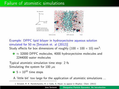
64 DPPC lipid molecules8 Hydroxyectoine molecules4488 SPC/E water molecules
Hydroxyectoine DPPC molecules Water
Example: DPPC lipid bilayer in hydroxyectoine aqueous solutionsimulated for 50 ns [Smiatek et. al (2012)]Study effects for box dimensions of roughly (100× 100× 10) nm3:
≈ 32000 DPPC molecules, 4000 hydroxyectoine molecules and2244000 water molecules
Typical atomistic simulation time step: 2 fsSimulating the system for 100 µs:
5× 10¹⁰ time steps
A ’little bit’ too large for the application of atomistic simulations ...
J. Smiatek, R. K. Harishchandra, H.-J. Galla, A. Heuer, to appear in Biophys. Chem. (2012)
Jens Smiatek Dissipative Particle Dynamics: An Introduction

Alternative method: Coarse-graining
Several effects for macromolecules, membranes, colloids etc. occuron time and length scales that are not accessible to all-atomsimulations.
Most of the computation time is spent into solvent interactions:Negligible? No, not always. Solvent mediated effects (solvationproperties, hydrodynamic interactions etc.) are sometimes of maininterest
Way out of this dilemma:
Coarse-grain the solutes
bead-spring models for polymers
Coarse-grain the solvent
Continuum implicit solvent models (GBSA, ’Browniandynamics’)Solve field theory on a grid (e. g. Lattice-Boltzmann)Real-space renormalization of solvent particles (DPD, SRD,SPH ...)
Jens Smiatek Dissipative Particle Dynamics: An Introduction

Solvent renormalization procedure
Atomistic solvent particles
Renormalization
DPD particles
DPD particle represents group of solvent molecules
molecules are smeared out: corresponding DPD potential should be”soft”
friction between particles to include dissipation
Jens Smiatek Dissipative Particle Dynamics: An Introduction

What about hydrodynamics and coarse-graining?
Acceleration of enclosed area: sum of forces over the boundary
Condition leads to Navier-Stokes equation
Jens Smiatek Dissipative Particle Dynamics: An Introduction

A small remark...
Coarse-graining means ...
... a reduction of the degrees of freedom for particles
... an acceleration of computation times
... maybe an oversimplification of the system
... a neglect of atomistic details
Not everything can be coarse-grained in a simple way...
Example:
MARTINI: coarse-grained force-field biases raft formation in lipid bilayers
in contrast to all-atom models [Hakobyan & Heuer (2012)]
D. Hakobyan, A. Heuer, to appear in Proc. Nat. Acad. Sci. USA (2012)
Jens Smiatek Dissipative Particle Dynamics: An Introduction

Particle based coarse-grained approach: Must haves
Characteristics and obligatory features of a meaningful method whichincludes hydrodynamic interactions and solvation effects:
Pair-wise conservative force to generate local thermodynamics(otherwise interpretation as an ideal gas)
Pair-wise dissipative force to model the viscosity on the mesoscale
Pair-wise random forces to include Brownian motion
Fluctuation-dissipation relation should hold for the generation of acanonical ensemble (NVT)
All forces should obey Newtons 3rd law (conservation of momentum)
Dissipative Particle Dynamics
Jens Smiatek Dissipative Particle Dynamics: An Introduction

Dissipative Particle Dynamics: History
Baby years (1992-1995):
1992: First introduction by Hoogerbrugge and KoelmanViolation of fluctuation-dissipation relation → no consistentensemble
Hype years (1995-2003)
1995: Correction of fluctuation-dissipation relation by Espanoland Warren1995-1999: Important contributions to the methodology byEspanol, Warren, Marsh, Yeomans, Lowe, Pagonabarraga,Groot, Alvares and othersOften used for colloidal systems, polymers, monolayers,mixtures, membranes ...
After the gold rush (2003-now):
What remains: useful for several systems to study varyingsolvent conditionsBut: ”Out of fashion” compared to Lattice-Boltzmann orStochastic rotation dynamics → computationally moreexpensive and slower
Jens Smiatek Dissipative Particle Dynamics: An Introduction

Dissipative Particle Dynamics equations
DPD-Forces:
~FDPDi =
∑
i 6=j~FDij + ~FR
ij
Dissipative force: ~FDij = −γDPD ωDPD(rij) (rij · ~vij) · rij
Random force: ~FRij =
√
2γDPD kBTωDPD(rij) χij · rij
rij distance and rij unit vector between two particles with relativevelocity vij within a cut-off distance rc
friction coefficient γDPD
symmetric random number χij = χji with zero mean and unitvariance
weight function
ωDPD(rij) =
{
1−rijrc
: rij ≤ rc0 : rij > rc
Jens Smiatek Dissipative Particle Dynamics: An Introduction

Conservative force
What about the conservative force?Often used:
~FCij = aij(1− rij/rc)
Parameter aij regulates strength of repulsive force and solvationproperties
Linear behavior
Allows large time steps
Requirement of a ”soft potential” due to smeared out molecular positionsis fulfilled.
A small hidden note ...Sometimes Lennard-Jones potentials are also in use ...
It is not forbidden!
Jens Smiatek Dissipative Particle Dynamics: An Introduction

Complete set of DPD forces
~FDPDi =
∑
i 6=j~FDij + ~FR
ij + ~FCij
Pairwise additive forces
Constructed to conserve local momentum in all force contributions
Can be integrated by an ordinary integration scheme (Verlet or morerefined self-consistent methods ...)
Jens Smiatek Dissipative Particle Dynamics: An Introduction

Thermodynamic ensemble: Fluctuation-Dissipation relation
A meaningful method should reproduce the equilibrium distribution of athermodynamic ensemble...
Probability to find system at a particular state: ρ(r3N , p3N)
Time evolution can be expressed by the Liouville equation:
∂∂t ρ(r
3N , p3N) = iLρ(r3N , p3N)
with
Liouville operator L = LC + LD (conservative (C) and dissipativecontributions (D))
Condition for a stable equilibrium distribution:
∂∂t ρ(r
3N , p3N) = 0
Jens Smiatek Dissipative Particle Dynamics: An Introduction

Conservative and dissipative contributions
Conservative contribution:
LCρ(r3N , p3N) = 0 (always fulfilled for conservative interactions)
Dissipative contribution:
LDρ(r3N , p3N) = 0 only fulfilled for
ωR(rij)2 = ωD(rij) [Espanol & Warren (1995)]
(condition for weight function in the dissipative and therandom contribution for the DPD equations)
ωR(rij) ... kinetic energy input per timeωD(rij) ... kinetic energy dissipation per time
The above relation was violated in the original paper by Hoogerbrugge
and Koelman...
P. Espanol, P. B. Warren, Europhys. Lett. 30, 191 (1995)
P. J. Hoogerbrugge, J. M. V. A. Koelman, Europhys. Lett. 19, 155 (1992)
Jens Smiatek Dissipative Particle Dynamics: An Introduction
Parameterisation of DPD
Problem:
Length scales are larger than atomistic scales
What is the behavior of the physical properties and how to match?
Requirement:
DPD solvent intends to reproduce the properties of atomisticsolutions as far as possible (local thermodynamics)
compressibility and densitytransport properties
Jens Smiatek Dissipative Particle Dynamics: An Introduction
Compressibility - matching aij
The equation of state at high density (ρ ≥ 2σ−3) can be expressed by
p = ρkBT + αρ2 (virial expansion with pressure p and density ρ)
The standard soft potential gives by matching with experimental oratomistic results
α ∼ 0.1aij r4c
Taking the dimensionless compressibility of water (κ−1 ∼ 16) intoaccount:
κ−1 = 1kBT
∂p∂ρ
= 1kBT
∂p∂n
∂n∂ρ
For κ−1 ∼ 16
aij = 75 kBTρr4c
[Groot & Warren (1997)]
Due to the purely repulsive force: no liquid-vapour coexistence!
R. D. Groot, P. B. Warren, J. Chem. Phys. 107, 4423 (1997)
Jens Smiatek Dissipative Particle Dynamics: An Introduction

A remark on the density
An increase of the solvent density will give better statistics but iscomputationally more expensive.Problems for low densities:
low collision frequency (more a gas than a liquid)
In more detail: Boltzmann two-particle collisions instead of manyparticle collisions [Schiller (2005)]
Detailed investigations on boundary conditions and shear viscosity inabsence of conservative forces have shown [Schiller (2005), Smiatek et.al (2008)]:
interplay between density ρ and friction coefficient γDPD
acceptable fluid like behavior for ρ ≥ 3σ−3 andγDPD = 5− 10
√
(mǫ/σ2)
U. D. Schiller, Diploma thesis, Bielefeld University, 2005
J. Smiatek, M. P. Allen, F. Schmid, Europ. Phys. J. E 26, 115 (2008)
Jens Smiatek Dissipative Particle Dynamics: An Introduction
Transport properties - Shear viscosity
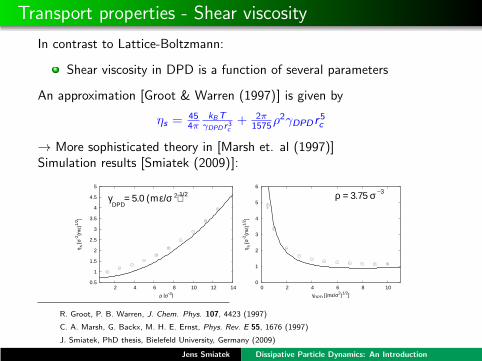
In contrast to Lattice-Boltzmann:
Shear viscosity in DPD is a function of several parameters
An approximation [Groot & Warren (1997)] is given by
ηs =454π
kBTγDPD r3c
+ 2π1575ρ
2γDPDr5c
→ More sophisticated theory in [Marsh et. al (1997)]Simulation results [Smiatek (2009)]:
0.5
1
1.5
2
2.5
3
3.5
4
4.5
5
2 4 6 8 10 12 14
η s [σ
-2(m
ε)1/
2 ]
ρ [σ-3]
0
1
2
3
4
5
6
0 2 4 6 8 10
η s [σ
-2(m
ε)1/
2 ]
γDPD [(mε/σ2)1/2]
DPD
1/2 ρ = 3.75 σ−3m γ = 5.0 ( ε/σ )2
R. Groot, P. B. Warren, J. Chem. Phys. 107, 4423 (1997)
C. A. Marsh, G. Backx, M. H. E. Ernst, Phys. Rev. E 55, 1676 (1997)
J. Smiatek, PhD thesis, Bielefeld University, Germany (2009)
Jens Smiatek Dissipative Particle Dynamics: An Introduction

Intrinsic properties: Schmidt number
The Schmidt number Sc denotes the ratio between momentum transportand mass transport with diffusion constant D:
Sc = ηs
ρD
Typical values in real fluids: 102 − 103
Inserting typical values for DPD:
Sc << 100
Diffusive transport is as fast as momentum transport→ DPD is more a gas than a liquid
No problem for Stochastic Rotation Dynamics, Lowe-Andersen
thermostat or Lattice-Boltzmann.
Jens Smiatek Dissipative Particle Dynamics: An Introduction

Further well-known problems
Too large time steps (δt > 0.01) result in wrong temperatures andequilibrium properties [Marsh & Yeomans (1997)]
Sound velocity too low for large bead sizes
Clash of intrinsic length scales (surfactants, micelles, oil droplets)
Lattice-Boltzmann and Stochastic Rotation Dynamics arecomputationally faster
DPD vs. LB (4320 solvent particles vs. 1728 solvent nodes onan Athlon c© MP2200+ CPU) [Smiatek et. al (2009)]LB is 9-10 times faster!Forget about comparisons with GPU codes ...
C.A. Marsh, J.M. Yeomans, Europhys.Lett. 37, 511 (1997)
J. Smiatek, M. Sega, U. D. Schiller, C. Holm, F. Schmid, J. Chem. Phys. 130, 244702 (2009)
Jens Smiatek Dissipative Particle Dynamics: An Introduction

Why choosing DPD as a method of choice?
There are many problems and it is computationally very slow ...
Why using DPD?
Solvent is modeled explicitly
gives probability to vary between good, theta and poor solventformation of compounds due to solvophobic interactions(membranes, vesicles and micelles)study of Flory-Huggins behavior (mixtures)
wall slippage for microchannel flows is well defined
Jens Smiatek Dissipative Particle Dynamics: An Introduction
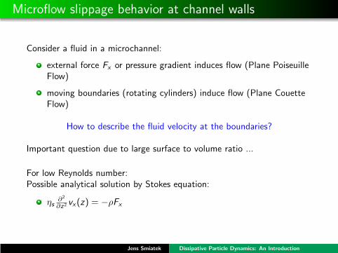
Microflow slippage behavior at channel walls
Consider a fluid in a microchannel:
external force Fx or pressure gradient induces flow (Plane PoiseuilleFlow)
moving boundaries (rotating cylinders) induce flow (Plane CouetteFlow)
How to describe the fluid velocity at the boundaries?
Important question due to large surface to volume ratio ...
For low Reynolds number:Possible analytical solution by Stokes equation:
ηs∂2
∂z2 vx(z) = −ρFx
Jens Smiatek Dissipative Particle Dynamics: An Introduction
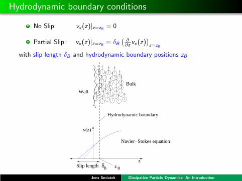
Hydrodynamic boundary conditions
No Slip: vx(z)|z=zB = 0
Partial Slip: vx(z)|z=zB = δB(
∂∂z vx(z)
)
z=zB
with slip length δB and hydrodynamic boundary positions zB
z
Wall
Bulk
v(z)
δB Bz
Navier−Stokes equation
Hydrodynamic boundary
Slip length
Jens Smiatek Dissipative Particle Dynamics: An Introduction

Modelling hydrodynamic boundary conditions inmicrochannels
Idea:
Introduction of a viscous layer (described in terms of a Langevinequation) with finite range zc in close vicinity to the channel walls
Wall velocity as a reference velocity(Moving walls for the simulation of shear flows)
LJ−interaction range
x
Viscous layer
Fluid particles
Channel walls
z
Jens Smiatek Dissipative Particle Dynamics: An Introduction

Typical flow profiles with Tunable-Slip Boundaries
0
0.2
0.4
0.6
0.8
1
1.2
-5 -4 -3 -2 -1 0 1 2 3 4 5
v x(z
)/v x
,max
(z)
z [σ]
Parabolic fit
-0.6
-0.4
-0.2
0
0.2
0.4
0.6
-5 -4 -3 -2 -1 0 1 2 3 4 5
v x(z
)/V
x
z [σ]
Linear fit
Range of Tunable−Slip Boundaries
Range of effective wall−particle interactions
Combination of both flow profiles for different parameter sets allows the
calculation of the slip length and of the hydrodynamic boundary positions
independently.
Jens Smiatek Dissipative Particle Dynamics: An Introduction
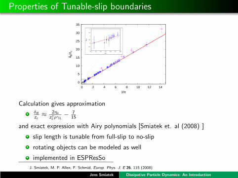
Properties of Tunable-slip boundaries
0
5
10
15
20
25
30
35
0 2 4 6 8 10 12 14
δ B/z
c
1/α
-1
-0.5
0
0.5
1
1.5
2
0.2 0.3 0.4 0.5 0.6 0.7 0.8
δ B/z
c
1/α
Calculation gives approximationδBzc
≈ 2ηs
z2c ργL− 7
15
and exact expression with Airy polynomials [Smiatek et. al (2008) ]
slip length is tunable from full-slip to no-slip
rotating objects can be modeled as well
implemented in ESPResSo
J. Smiatek, M. P. Allen, F. Schmid, Europ. Phys. J. E 26, 115 (2008)
Jens Smiatek Dissipative Particle Dynamics: An Introduction

Dissipative Particle Dynamics in ESPResSo
Jens Smiatek Dissipative Particle Dynamics: An Introduction

Several ways to treat DPD in ESPResSo
ESPResSo treats DPD either as ...
a global thermostat with no specified conservative interaction (idealgas [Soddemann et al. (2003)])
or a thermostat with specified DPD interactions
T. Soddemann, B. Dunweg, K. Kremer, Phys. Rev. E 68, 046702 (2003)
Jens Smiatek Dissipative Particle Dynamics: An Introduction

Setting up a DPD thermostat simulation
In myconfig.h:#define DPDIn the TCL-Script:...for{set i 0}{$i < N}{incr i}{set posx [expr $box x*[t random]]...part $i pos $posx $posy $posz type $solvent id v $vx $vy $vz}galileiTransformParticles...set temperature 1.0set gamma 1.0set r cut 1.0thermostat dpd $temperature $gamma $r cut
...
Jens Smiatek Dissipative Particle Dynamics: An Introduction

DPD thermostat simulation plus DPD interaction
In myconfig.h:#define inter DPDIn the TCL-Script:...for{set i 0}{$i < N}{incr i}{set posx [expr $box x*[t random]]...part $i pos $posx $posy $posz type $solvent id v $vx $vy $vz}galileiTransformParticles...set temperature 1.0set gamma 1.0set r cut 1.0thermostat inter dpd $temperature $gamma $r cutinter $solvent id $solvent id inter dpd $gamma $r cut
...
Jens Smiatek Dissipative Particle Dynamics: An Introduction

Extension: Transverse DPD and mass dependent friction
Transverse DPD:
Dampens the degrees of freedom perpendicular on the axisbetween two particles [Junghans et. al (2008)]
In myconfig.h:#define TRANS DPD
Mass-dependent friction:
In myconfig.h:#define DPD MASS RED or #define DPD MASS LIN
for γDPD → γDPDMij
with reduced mass Mij = 2mimj/mi +mj
with average mass Mij = 1/2(mi +mj)
C. Junghans, M. Praprotnik, K. Kremer, Soft Matter 4, 156 (2008)
Jens Smiatek Dissipative Particle Dynamics: An Introduction

Further remarks
Integration via Velocity-Verlet algorithm → δt ≤ 0.01 [Marsh &Yeomans (1997)]
Never forget to set galileiTransformParticles because it removes boxcenter of mass motion
C.A. Marsh, J.M. Yeomans, Europhys.Lett. 37, 511 (1997)
Jens Smiatek Dissipative Particle Dynamics: An Introduction

Main applications:Solvation properties and flow profiles
I. Solvation properties of polymers
Jens Smiatek Dissipative Particle Dynamics: An Introduction

Polymers in solution [Spenley (2000)]
End-to-end radius re ∼ Nνwith N monomers
Theory: ν = 0.588
DPD simulation: ν = 0.58± 0.04 for re ∼ (N − 1)ν
Relaxation time of end-to-end distance τ ∼ r3e ∼ N3ν
Theory: 3ν = 1.77
DPD simulation: 3ν = 1.80± 0.04
Good reproduction of hydrodynamic properties (Zimm-regime) and staticproperties of the polymer
N. A. Spenley, Europhys. Lett. 49, 534 (2000)
Jens Smiatek Dissipative Particle Dynamics: An Introduction

Polymers in melt [Spenley (2000)]
End-to-end radius re ∼ Nνwith N monomers
Theory: ν = 0.5
DPD simulation: ν = 0.498± 0.005 for re ∼ (N − 1)ν
Relaxation time of end-to-end distance τ ∼ Nβ
Theory: β = 2
DPD simulation: β = 1.98± 0.03
Good reproduction of screening properties (Rouse-regime) and staticproperties of the polymer
N. A. Spenley, Europhys. Lett. 49, 534 (2000)
Jens Smiatek Dissipative Particle Dynamics: An Introduction

Influence of solvent conditions for polymer translocationtimes [Kapahnke et. al (2010)]
Solvent conditions influence the time scaling behavior for anunbiased polymer translocation process
Decreasing solvent quality by increasing aij values
Theory: Translocation time τ ∼ Nβ with β = 1 + 2ν = 2.2 for goodsolvent conditions
∆aij ν β
0 (good solvent) 0.60± 0.00(0.588) 2.24± 0.03(2.16)
6 0.57± 0.01 2.22± 0.03
12 0.44± 0.01 2.09± 0.08
17 0.27± 0.02 1.98± 0.08
Reproduction of polymer collapse and change of translocation times
F. Kapahnke, U. Schmidt, D. W. Heermann, M. Weiss, J. Chem. Phys. 132, 164904 (2010)
Jens Smiatek Dissipative Particle Dynamics: An Introduction
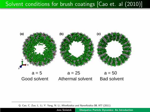
Solvent conditions for brush coatings [Cao et. al (2010)]
Good solvent Athermal solvent Bad solventa = 5 a = 25 a = 50
Q. Cao, C. Zuo, L. Li, Y. Yang, N. Li, Mirofluidics and Nanofluidics 10, 977 (2011)
Jens Smiatek Dissipative Particle Dynamics: An Introduction
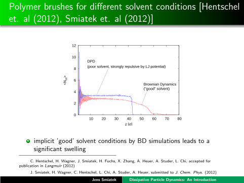
Polymer brushes for different solvent conditions [Hentschelet. al (2012), Smiatek et. al (2012)]
0
2
4
6
8
10
12
10 20 30 40 50 60 70 80
<N
m>
z [σ]
Brownian Dynamics("good" solvent)
DPD(poor solvent, strongly repulsive by LJ potential)
implicit ’good’ solvent conditions by BD simulations leads to asignificant swelling
C. Hentschel, H. Wagner, J. Smiatek, H. Fuchs, X. Zhang, A. Heuer, A. Studer, L. Chi, accepted forpublication in Langmuir (2012)
J. Smiatek, H. Wagner, C. Hentschel, L. Chi, A. Studer, A. Heuer, submitted to J. Chem. Phys. (2012)
Jens Smiatek Dissipative Particle Dynamics: An Introduction

Main applications:Solvation properties and flow profiles
II. Flow profiles in microchannels
Jens Smiatek Dissipative Particle Dynamics: An Introduction
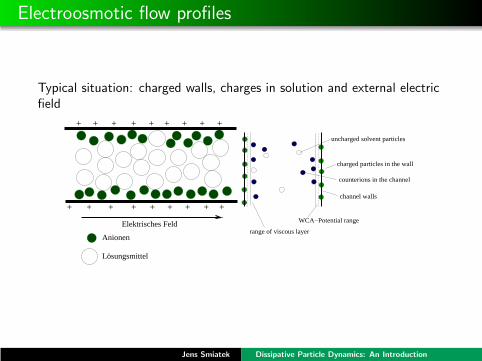
Electroosmotic flow profiles
Typical situation: charged walls, charges in solution and external electricfield
+ + + + + +
+ + + + + ++ ++
+ + +
Elektrisches Feld
Anionen
Lösungsmittel
uncharged solvent particles
charged particles in the wall
counterions in the channel
channel walls
range of viscous layer
WCA−Potential range
Jens Smiatek Dissipative Particle Dynamics: An Introduction
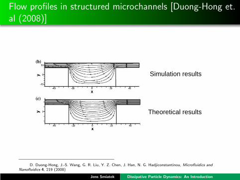
Flow profiles in structured microchannels [Duong-Hong et.al (2008)]
Simulation results
Theoretical results
D. Duong-Hong, J.-S. Wang, G. R. Liu, Y. Z. Chen, J. Han, N. G. Hadjiconstantinou, Microfluidics andNanofluidics 4, 219 (2008)
Jens Smiatek Dissipative Particle Dynamics: An Introduction
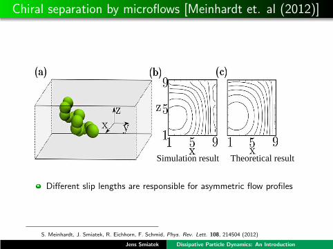
Chiral separation by microflows [Meinhardt et. al (2012)]
Simulation result Theoretical result
Different slip lengths are responsible for asymmetric flow profiles
S. Meinhardt, J. Smiatek, R. Eichhorn, F. Schmid, Phys. Rev. Lett. 108, 214504 (2012)
Jens Smiatek Dissipative Particle Dynamics: An Introduction

Chiral separation by microwflows [Meinhardt et. al (2012)]
S. Meinhardt, J. Smiatek, R. Eichhorn, F. Schmid, Phys. Rev. Lett. 108, 214504 (2012)
Jens Smiatek Dissipative Particle Dynamics: An Introduction

Counterion-induced electroosmotic flow [Smiatek et. al(2009)]
Counterion densities:
0
0.05
0.1
0.15
0.2
0.25
0.3
-4 -3 -2 -1 0 1 2 3 4
Ion
Den
sity
ρ [σ
-3]
z [σ]
J. Smiatek, M. Sega, U. D. Schiller, C. Holm, F. Schmid, J. Chem. Phys. 130, 244702 (2009)
Jens Smiatek Dissipative Particle Dynamics: An Introduction

Counterion-induced electroosmotic flow [Smiatek et. al(2009)]
Electrosmotic flow profiles for different slip lengths:
0
0.05
0.1
0.15
0.2
0.25
0.3
0.35
0.4
0.45
-4 -3 -2 -1 0 1 2 3 4
v x(z
)/E
x [e
σ(m
ε)-1
/2]
z [σ]
δ = 0.782 σ
δ = 0.248 σ
δ = 0.000 σB
B
B
Bδ = 1.399 σ
J. Smiatek, M. Sega, U. D. Schiller, C. Holm, F. Schmid, J. Chem. Phys. 130, 244702 (2009)
Jens Smiatek Dissipative Particle Dynamics: An Introduction
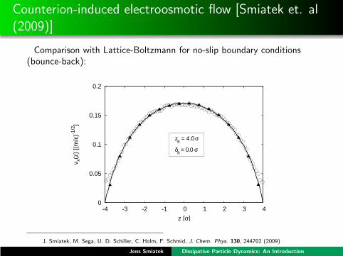
Counterion-induced electroosmotic flow [Smiatek et. al(2009)]
Comparison with Lattice-Boltzmann for no-slip boundary conditions(bounce-back):
0
0.05
0.1
0.15
0.2
-4 -3 -2 -1 0 1 2 3 4
v x(z
) [(
m/ε
)-1/2
]
z [σ]
z = 4.0 B
σ
δ = 0.0 σB
J. Smiatek, M. Sega, U. D. Schiller, C. Holm, F. Schmid, J. Chem. Phys. 130, 244702 (2009)
Jens Smiatek Dissipative Particle Dynamics: An Introduction
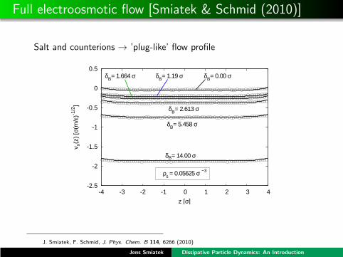
Full electroosmotic flow [Smiatek & Schmid (2010)]
Salt and counterions → ’plug-like’ flow profile
-2.5
-2
-1.5
-1
-0.5
0
0.5
-4 -3 -2 -1 0 1 2 3 4
v x(z
) [σ
(m/ε
)-1/2
]
z [σ]
δ = 14.00 σ
ρ = 0.05625 σs−3
B
B
B
B B B
δ = 5.458 σ
δ = 2.613 σ
δ = 1.664 σ δ = 1.19 σ δ = 0.00 σ
J. Smiatek, F. Schmid, J. Phys. Chem. B 114, 6266 (2010)
Jens Smiatek Dissipative Particle Dynamics: An Introduction
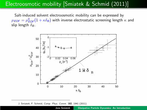
Electroosmotic mobility [Smiatek & Schmid (2011)]
Salt-induced solvent electroosmotic mobility can be expressed byµEOF = µ0
EOF (1 + κδB) with inverse electrostatic screening length κ andslip length δB .
0
10
20
30
40
50
0 10 20 30 40 50
µ EO
F /
µ EO
F
ρs [σ-3]
0
κ δB
1 + κ δ B
-2
-1
0
0 0.02 0.04 0.06
ψB [k
BT
/e]
J. Smiatek, F. Schmid, Comp. Phys. Comm. 182, 1941 (2011)
Jens Smiatek Dissipative Particle Dynamics: An Introduction
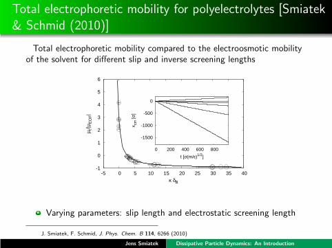
Total electrophoretic mobility for polyelectrolytes [Smiatek& Schmid (2010)]
Total electrophoretic mobility compared to the electroosmotic mobilityof the solvent for different slip and inverse screening lengths
-1
0
1
2
3
4
5
6
-5 0 5 10 15 20 25 30 35 40
µ t/|µ
EO
F|
κ δB
-1500
-1000
-500
0
0 200 400 600 800
x cm
[σ]
t [σ(m/ε)1/2]
Varying parameters: slip length and electrostatic screening length
J. Smiatek, F. Schmid, J. Phys. Chem. B 114, 6266 (2010)
Jens Smiatek Dissipative Particle Dynamics: An Introduction

Center-of-mass motion for polyelectrolytes [Smiatek &Schmid (2010)]
-1500
-1000
-500
0
0 200 400 600 800
x cm
[σ]
t [σ(m/ε)1/2]
δ = 14.00 σB
B
B
B B B
δ = 5.458 σ
δ =2.613 σ
δ = 1.664 σδ = 1.19 σδ = 0.00 σ
Boundary parameters are important: Change of direction due toEOF magnitude increase
J. Smiatek, F. Schmid, J. Phys. Chem. B 114, 6266 (2010)
Jens Smiatek Dissipative Particle Dynamics: An Introduction

Summary
Dissipative Particle Dynamics is a powerful tool to ...
qualitatively investigate solvation behavior
treat boundary conditions in microchannel flows
analyze mixing behavior of different species
Jens Smiatek Dissipative Particle Dynamics: An Introduction

References
Dissipative Particle Dynamics:
P. Espanol and P. B. Warren. Statistical mechanics of dissipative particledynamics. Europhys. Lett., 30, 191 (1995)
R. D. Groot and P. B. Warren. Dissipative particle dynamics: Bridging the gapbetween atomistic and mesoscopic simulation. J. Chem. Phys. 107, 4423 (1997)
E. Moeendabary, T. Y. Ng and M. Zangeneh. Dissipative particle dynamics:Introduction, Methodology and complex fluid applications - a review. Int. J.Appl. Mechanics 1, 737 (2009)
Electrokinetic phenomena in combination with coarse-grained methods:
G. W. Slater, C. Holm, M. V. Chubynsky, H. W. de Haan, A. Dube, K. Grass,O. A. Hickey, C. Kingsburry, D. Sean, T. N. Shendruk, L. Zhan. Modeling theseparation of macromolecules: A review of current computer simulationmethods. Electrophoresis 30, 792 (2009)
I. Pagonabarraga, B. Rotenberg and D. Frenkel. Recent advances in themodelling and simulation of electrokinetic effects: Bridging the gap betweenatomistic and macroscopic descriptions. Phys. Chem. Chem. Phys. 12, 9566(2010)
J. Smiatek and F. Schmid. Mesoscopic simulation methods for studying flowand transport in electric fields in micro- and nanochannels. Advances inMicrofluidics. R. T. Kelly (Ed.) InTech. (2012)
Jens Smiatek Dissipative Particle Dynamics: An Introduction
Acknowledgements
I have to thank ...
Prof. Dr. Friederike Schmid (University of Mainz)
Prof. Dr. Andreas Heuer (University of Munster)
Prof. Dr. Christian Holm (University of Stuttgart)
Collaborations:
Prof. Dr. Michael P. Allen (University of Warwick)
Dr. Marcello Sega (University of Rome ’Tor Vergata’)
Dr. Ulf D. Schiller (FZ Julich) and Prof. Dr. Burkhard Dunweg(MPI-P Mainz)
Computing time:
ARMINIUS-Parallel-Cluster at Paderborn University, NIC Julich,HLRS Stuttgart, PALMA-Cluster Munster
Funding:
Volkswagen-Stiftung and Deutsche Forschungsgemeinschaft
Jens Smiatek Dissipative Particle Dynamics: An Introduction

Acknowledgements
All our simulations have been carried out by the software package
http://www.espressomd.org
Thank you for your attention!
Jens Smiatek Dissipative Particle Dynamics: An Introduction