dissertation propagation of the sidoardjo mud in the
TRANSCRIPT
DISSERTATION
PROPAGATION OF THE SIDOARDJO MUD IN THE PORONG RIVER, EAST JAVA, INDONESIA
Submitted by
Neil Andika
Department of Civil and Environmental Engineering
In partial fulfillment of the requirements
For the Degree of Doctor of Philosophy
Colorado State University
Fort Collins, Colorado
Summer 2021
Doctoral Committee:
Advisor: Pierre Y. Julien
Neil S. Grigg
Robert Ettema
Sara Rathburn

Copyright by Neil Andika 2021
All Rights Reserved

ii
ABSTRACT
PROPAGATION OF THE SIDOARDJO MUD IN THE PORONG RIVER, EAST JAVA, INDONESIA
The Sidoarjo Mud Volcano in East Java, Indonesia erupted on May 29, 2006. It caused controversy
because of the impact of the mud volcano had on communities around it. The discharge of the mud
volcano was 50,000 m3/d (Harnanto, 2011) which comprised a 35% concentration of silt and clay.
To mitigate the damage to surrounding regions, the Government of Indonesia diverted the mud to
Madura Strait through the Porong River in 2016 (Hadimuljono, 2008). The objectives of this thesis
are to: (1) understand the physical properties of mud from the mud volcano and its interaction with
the water in the river; (2) carry out field measurements of sediment concentration along the Porong
River for a model validation; (3) determine how the concentration of mud from the mud volcano
varies along the river; (4) create a framework or guideline for the mitigation of a mud volcano
disaster in the future.
Laboratory experiments were used to test the sediment properties. The experiments of turbidity
and sediment concentration, 𝐶, concluded that the linear regression, 𝐶 = 5.297 × 𝑇𝑢𝑟𝑏𝑖𝑑𝑖𝑡𝑦 +
24, was the best fitted regression. Flocculation tests in 2019 showed that the recorded
deflocculated settling velocity for the sample of the Ginonjo Outlet was 0.013 mm/s which was
approximately 2 times slower than the natural settling velocity of 0.028 mm/s. This value was one
order slower than the general settling velocity for flocculated particles.
Two field measurement programs were completed, in July 2018 and in September 2019. The field
programs in 2018 observed the sediment concentration along the Porong River at 106 cross-

iii
sections and the point source sediment concentration at Ginonjo Outlet was 57,000 mg/l. It was
found that the observed maximum sediment concentration ranged between 691 mg/l and 4,198
mg/l. The average sediment concentration at the downstream end of the Porong River on the other
hand was 90 mg/l. The field program in 2019 captured the vertical sediment concentration profiles
of the first 4 km of the Porong River. The highest near-bed sediment concentration was 1,500 mg/l
at Line C cross-section 9. This was followed by 1,450 mg/l at Line C cross-section 6. These
measurements showed that the sediment concentration are uniform along the Porong River except
for the first 4 km where the bottom sediment concentration are higher.
There are three flow conditions based on the hydrograph of the Porong River: low flow with 45
m3/s, medium flow with 250 m3/s, and high flow with 2500 m3/s. For low flow, the average flow
velocity was 0.12 m/s and the shear velocity was 0.01 m/s. Results from the two-dimensional
mixing model without settling was the fully-mixed concentration for low flow condition achieved
at 4 km downstream from the outlet with a concentration of 470 mg/l. There was 380 mg/l
difference between the model’s result and the observed concentration.
The two-dimensional mixing and setting model without flocculation produced a result of sediment
concentration of 195 mg/l at the downstream end of the Porong River. This came from the clay
fraction which was about 48% of the total sediment. The sediment concentration difference
between this model and the observed data was 105 mg/l. The two-dimensional mixing and setting
model with flocculation was then used. The sediment concentration at the left bank side of the
Porong River was about 90 mg/l, which matched the observed data. The gravel, sand and coarser
silt fractions settled at the first 4 km of the study reach was also captured by the model. This result
proved that the two-dimensional mixing and settling model with flocculation was a suitable model
for the sediment propagation in Porong River.

iv
ACKNOWLEDGEMENTS
All prise be to Allah, The One Almighty God and The Exalted. Because of His unlimited kindness,
love, mercy, and guidance, I was able to finish this dissertation. Peace and salutation are uttered
to our beloved Prophet Muhammad Peace Be Upon Him who has broung humanity to the light of
Islam.
First and foremost, I am very grateful to Dr. Pierre Y. Julien as my advisor who gave me unending
encouragement, helpful advice, and support throughout my Ph.D. program since 2015. I would
like to thank the committee member: Dr. Neil S. Grigg, Dr. Robert Ettema, and Dr. Sara Rathburn
for their outstanding contribution to this research. Also, I would like to thank CSU faculty
including Dr. Timothy Gates, Dr. Darrell Fontane, Dr. Karan Venayagamoorthy, Dr. Mazdak
Arabi, and Dr. Ellen Wohl for their valuable classes. I would also thank Linda Hinshaw, Laurie
Alburn, and Susheela Mallipudi for their help and patience.
I am thankful for LPDP (Indonesia Endownment Fund for Education) for the financial support
from my Master program to the extension for my Ph.D. program. Also, I would like to thank PPLS
(Sidoardjo Mud Control Center – Indonesia) and Ministry of Public Work and Housing of the
Republic of Indonesia for their help and assistance for my research.
I would like to send my gratitude for all my research mate and class mate including Marcos Palu,
Chunyao Yang, Woochul Kang, Hwa Young Kim, Susan Cundiff, Weimin Li, Kristin LaForge,
Kennard Lai, Corinne Horner, Tori Beckwith, Caitlin Fogarty, Dr. Jai Hong Lee, Dr. Seongjoon
Byeon, Dr. Joonhak Lee, Dr. Eunkyung Jang, and Dr. Xudong Chen. I will miss our Seminar
Series.

v
I am very thankful to my Indonesian friends in Fort Collins: Faizal Rohmat and Winda, Brandon
Bernandus, Gabriel Kereh, Bagus Mahardika, Owen Carniege Limarta, Dhira Prasanti, Eka
Noviana, Monika Aprianti, Aya Safira, Adji Witjaksono, Demison Tabuni, and all members of
Permias Fort Collins for their friendship. We will conquer Indonesia together in near future. I
would like to extend my gratitude to Mas Setyo Nugroho and Mbak Hesti, Mas Anton Pratama,
Mbak Dessy Sapardina, Mas Ahmadin, and all Indonesian in Colorado for their support since I
arrived in Colorado.
Finally, my deepest thanks to my beloved family, especially my parents M Basuki Hadimuljono
and Kartika Nurani, my wife Aziza Widyani, my brothers and sisters, and all of my family
members. Thank you for keep believing in me and keep giving me support. I love you all!

vi
TABLE OF CONTENTS
ABSTRACT .................................................................................................................................... ii
ACKNOWLEDGEMENTS ........................................................................................................... iv
LIST OF TABLES ......................................................................................................................... ix
LIST OF FIGURES ........................................................................................................................ x
CHAPTER 1 Introduction ........................................................................................................... 1
1.1 Background ...................................................................................................................... 1
1.2 Problem Statement ........................................................................................................... 3
1.3 Research Objective ........................................................................................................... 4
CHAPTER 2 Literature Review .................................................................................................. 6
2.1 Mud Volcano .................................................................................................................... 6
2.2 Clay mineralogy ............................................................................................................... 9
2.3 Sidoardjo Mud Volcano ................................................................................................. 13
2.4 Mud Properties ............................................................................................................... 16
2.5 Sediment Transport in Rivers ......................................................................................... 25
CHAPTER 3 Site Description ................................................................................................... 38
3.1 Sidoardjo Mud Reservoir ............................................................................................... 38
3.2 Porong River .................................................................................................................. 43
CHAPTER 4 The Properties of the Diverted Mud .................................................................... 51

vii
4.1 Particle Size Distribution of Mud Samples .................................................................... 51
4.2 The Relationship of Turbidity and Sediment Concentration ......................................... 53
4.3 Flocculation .................................................................................................................... 56
CHAPTER 5 Field Measurements ............................................................................................ 60
5.1 Field Measurement Program #1 (July 10-14, 2018) ...................................................... 60
5.2 Field Measurement Program #2 (September 10-12, 2019) ............................................ 62
CHAPTER 6 Sediment Propagation Model for the Porong River ............................................ 71
6.1 HEC-RAS ....................................................................................................................... 71
6.2 Two-Dimensional Mixing Model................................................................................... 76
6.3 Two-Dimensional Mixing and Settling Model without Flocculation ............................ 86
6.4 Two-Dimensional Mixing and Settling Model with Flocculation ................................. 89
CHAPTER 7 Management ........................................................................................................ 94
7.1 Current Condition and Recommendation ....................................................................... 94
7.2 Mud Volcano Disaster Guidelines ................................................................................. 98
CHAPTER 8 Conclusions ....................................................................................................... 101
8.1 Properties of the Diverted Mud .................................................................................... 101
8.2 Field Measurements ..................................................................................................... 102
8.3 Sediment Propagation Model for Porong River ........................................................... 102
8.4 Mud Volcano Disaster Guidelines ............................................................................... 104
APPENDIX A ............................................................................................................................. 117

viii
APPENDIX B ............................................................................................................................. 120
APPENDIX C ............................................................................................................................. 127

ix
LIST OF TABLES
Table 1 Simulated growth of Sidoardjo Mud Volcano (after Istadi et al., 2009)......................... 15
Table 2 Summary of the relationship between turbidity and sediment concentration from previous
studies ........................................................................................................................................... 22
Table 3 The value of Manning’s coefficient (after Brunner, 2016) ............................................. 30
Table 4 Classification of the mode of sediment transport ............................................................ 33
Table 5 Hydraulic properties of the Porong River ....................................................................... 46
Table 6 The grain size and gradient coefficient of mud samples ................................................. 51
Table 7 Turbidity (NTU) of the sediment mixture of the corresponding sediment concentration
from the laboratory experiment in 2018 ....................................................................................... 54
Table 8 Summary of the analysis of sediment concentration parameter ...................................... 68
Table 9 Suspended sediment concentration parameters for 6 cross-sections in the study area ... 70
Table 10 Summary of the coefficitent, length and time scale of longitudinal dispersion, vertical
and transversal mixing of the Porong River ................................................................................. 76
Table 11 The classes of the diverted mud with its parameter and sediment concentration at certain
distance from the Ginonjo Outlet .................................................................................................. 91
x
LIST OF FIGURES
Figure 1 Mud flow drowned several settlements and infrastructures in Sidoardjo since 2006 ..... 2
Figure 2 The discharge of the mud mixture into the Porong River at the Pejarakan Outlet .......... 3
Figure 3 Structure of a conical mud volcano (from Dimitrov, 2002) ............................................ 7
Figure 4 The mud volcano distribution in the Bogor – North Serayu – Kendeng depression zone
(after Satyana and Asnidar, 2008) .................................................................................................. 8
Figure 5 Illustration of tetrahedron and tetrahedral sheel at top and octahedron and octahedral
sheet at bottom (Aboubakr et al. 2013) ........................................................................................... 9
Figure 6 Illustration of the silica structure for 1:1 clay mineral and 2:1 clay mineral (Sivakuga,
2001 at Marchuk, 2016) ................................................................................................................ 10
Figure 7 Swelling mechanism of smectite (Aniekan et al., 2018) ............................................... 11
Figure 8 Stratigraphy from Banjar Panji-1 exploration well in Sidoardjo, East Java (after Mazzini
et al., 2007) ................................................................................................................................... 14
Figure 9 Comparison of the observed and predicted suspended sediment concentration for (a) in-
situ calibration, and (b) laboratory calibration (after Minella et al., 2008) .................................. 20
Figure 10 The relationship of turbidity and suspended sediment concentration for 5 particle size
fractions prepared in dispersant and river water with S100 and S1000 optical turbidimeter (Foster
et al., 1992) ................................................................................................................................... 21
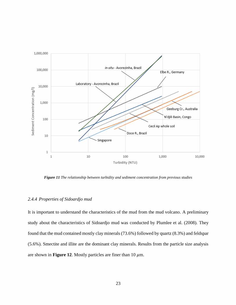
Figure 11 The relationship between turbidity and sediment concentration from previous studies
....................................................................................................................................................... 23
Figure 12 Particle size distribution of Sidoardjo mud (after USGS, 2008) ................................. 24
Figure 13 Illustration of additional channel boundaries (after Fischer et al., 1979) .................... 29
xi
Figure 14 Proposed method to determine Rouse number (after Akalin, 2002) ........................... 32
Figure 15 Sentinel-2 imagery of the Porong River in infrared (Bioresita et al., 2018) ............... 36
Figure 16 The location of Sidoardjo Mud Volcano ..................................................................... 38
Figure 17 The recent photos of Sidoardjo Mud Volcano: a) bird view of the mud reservoir with
the main crater in the circle; b) the main crater of the Sidoardjo Mud Volcano .......................... 39
Figure 18 The evolution of Sidoardjo Mud Volcano taken with Google Earth (from left to right
are pictures in 06/30/2006, 07/08/2010 and 08/07/2018, respectively) ........................................ 40
Figure 19 The 2016 Embankment maps of the mud reservoir ..................................................... 42
Figure 20 Plan view of the study reach in Porong River ............................................................. 43
Figure 21 Hourly discharges of the Porong River based on Porong Station from 2012 to 2016 44
Figure 22 Flow duration curve of the Porong River .................................................................... 45
Figure 23 Cross-section of the Porong River ............................................................................... 46
Figure 24 Location of the sampling of bed material in the Porong River, Sidoardjo, East Java . 47
Figure 25 Particle size distribution of bed materials of Porong River ......................................... 48
Figure 26 Temperature of the diverted mud from Ginonjo Outlet on September 12, 2020 ........ 49
Figure 27 Temperature of flow of the Porong River on September 12, 2020 ............................. 50
Figure 28 Temperature of flow of the Porong River on October 4-5 , 2020 ............................... 50
Figure 29 Particle size distribution of mud samples (VC: very coarse, C: coarse, M: medium, F:
fine, and VF: very fine) ................................................................................................................. 52
Figure 30 Regression analysis for turbidity and sediment concentration in Porong River in 2018
....................................................................................................................................................... 55
Figure 31 Comparison of the relationship of turbidity and sediment concentration between the
preliminary result and previous studies ........................................................................................ 56
xii
Figure 32 Samples from Pejarakan and Ginonjo Outlet. Sample from left: P1, P2, G1 and G2;
deflocculant were added to P2 and G2. ........................................................................................ 57
Figure 33 Results of flocculation test .......................................................................................... 58
Figure 34 Ratio of settling velocity of deflocculated samples and original samples ................... 59
Figure 35 Illustration of field measurement #1 in the study reach; not to scale (point A, B, C, and
D illustrated the 4 points of measurement in one cross-section) .................................................. 61
Figure 36 Water sampler horizontal for field measurements ....................................................... 61
Figure 37 Photos of the field measurements #1 ........................................................................... 62
Figure 38 The measured sediment concentration in the study reach ........................................... 63
Figure 39 Illustration of field measurement #2 in the study reach; not to scale (point A, B, C, and
D illustrated the 4 points of measurement in one cross-section) .................................................. 64
Figure 40 Photos of field measurements and bottles of samples ................................................. 64
Figure 41 The longitudinal sediment concentration per 1 m depth ............................................. 66
Figure 42 Plot of suspended sediment concentration versus (ℎ − 𝑧)/𝑧 ...................................... 67
Figure 43 Suspended sediment profiles for 6 cross-sections in the study area ............................ 69
Figure 44 Plan view of the study reach in HEC-RAS (GO is Ginonjo Outlet) ........................... 71
Figure 45 The cross-sections of the study reach .......................................................................... 72
Figure 46 Flow series of the study reach for 2012-2016 ............................................................. 73
Figure 47 Tides in Madura Strait ................................................................................................. 73
Figure 48 The sediment data of HEC-RAS simulation................................................................ 74
Figure 49 The water surface elevation of the study reach from HEC-RAS simulation (
indicates flow direction and GO is Ginonjo Outlet) ..................................................................... 75

xiii
Figure 50 Expected sediment propagation in left bank, centerline and right bank in Porong River
for three flow conditions ............................................................................................................... 78
Figure 51 Expected sediment concentration at 5km, 10 km and 15 km in Poromg River for three
flow conditions.............................................................................................................................. 80
Figure 52 Two-dimensional model without settling in the first 100 m of study reach for 3 flow
conditions ...................................................................................................................................... 82
Figure 53 Two-dimensional model without settling from 100 m to 15800 m of study reach for 3
flow conditions.............................................................................................................................. 83
Figure 54 Sediment propagation model without settling (Line A-D) and the field measurements
(meas.) ........................................................................................................................................... 85
Figure 55 The result from suspended sediment propagation model by size fraction at low flow (45
m3/s) without flocculation for Line A compared to the measurement data .................................. 88
Figure 56 The result from suspended sediment propagation model by size fraction at low flow (45
m3/s) without flocculation for Line A compared to the measurement data .................................. 90
Figure 57 Comparison of the measurement data, the result of model with flocculation at left bank,
centerline, and right bank, and the model without flocculation .................................................... 93
Figure 58 Residual plot for linear and power regression of turbidity – sediment concentration in
Porong River ............................................................................................................................... 118
Figure 59 The comparison of observed and predicted value of sediment concentration from
laboratory experiment ................................................................................................................. 119
Figure 60 Sediment time series of cross-section 46.................................................................... 127
Figure 61 Sediment time series of cross-section 39.................................................................... 127
Figure 62 Sediment time series of cross-section 32.................................................................... 128

xiv
Figure 63 Sediment time series of cross-section 27.................................................................... 128

1
CHAPTER 1 INTRODUCTION
1.1 Background
The Sidoardjo Mud Volcano erupted on May 29, 2006 in East Java, Indonesia. In 2007, the
eruption rate was 110,000 m3/d and the volumetric sediment concentration increased to 70%
(Mazzini et al., 2007). The average eruption rate had gradually decreased to 50,000 m3/d since
then (Harnanto, 2011). The Sidoardjo Mud Volcano, which is arguably the biggest onshore mud
volcano recorded, caused devastation to the surrounding area. The Sidoardjo Mud Volcano caused
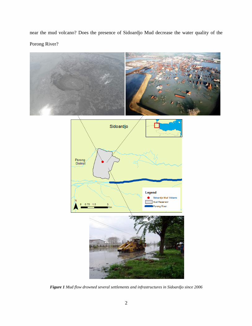
at least 30,000 people to flee their homes and become refugees (McMichael, 2009), buried 10,000
houses and forced about 23 companies to shut down, as shown in Figure 1. The total economic
loss based on data from the Ministry of Public Works of Indonesia report in 2007 was Rp 7.6
trillion, or about $565 million USD. On March 22, 2007, the impacted area, as determined by the
National Mudflow Disaster Management Team (Tim Nasional Penanggulangan Semburan
Lumpur Sidoardjo), was 650 ha.
A key issue was that the mud volcano was expected to flow at least until 2027 as the volume of
mud was found to be consistently increasing inside the reservoir. Thus, containment measure was
necessary. In addition, the Management Team discharged some portions of the mud to Madura
Strait through the Porong River since November 2006 (Hadimuljono, 2008). The diversion were
managed by Sidoardjo Mud Control Agency (or BPLS – Badan Penanggulangan Lumpur
Sidoardjo) from 2007, and continued by Sidoardjo Mud Control Center (or PPLS – Pusat
Pengendalian Lumpur Sidoardjo) from 2017. This catastrophic event raised several scientific and
technical questions regarding the interaction between mud volcanoes and fluvial systems in
heavily populated areas. Is the mud harmful to human health? Can human or living organism live
2
near the mud volcano? Does the presence of Sidoardjo Mud decrease the water quality of the
Porong River?
Figure 1 Mud flow drowned several settlements and infrastructures in Sidoardjo since 2006

3
1.2 Problem Statement
The Porong River flows approximately 2 km away from the creater of the mud volcano. Because
of its proximity, the river was used as a channel to transport the mud towards the Madura Strait.
The mud was diluted before it was discharged into the Porong River, as shown in Figure 2, to
reduce the sediment concentration into the Porong River. This action could change the river
dynamic, by increasing the sediment concentration and disturbing the fish and native wildlife along
the Porong River. In addition, this action also caused sedimentation in the Madura Strait. The
overall impact however, varied at different sediment concentrations depending on the discharged
mixture.
Figure 2 The discharge of the mud mixture into the Porong River at the Pejarakan Outlet

4
1.3 Research Objective
The overall objective of this research is to determine whether the diversion of the mud is a good
idea or not from the technical stand point. The primary concerns of this research are the increase
in the sediment concentration which includes: (1) turbidity over a range of discharges in the Porong
River; (2) the high concentration of fine sediment; and (3) the size of mud particles and its settling
processes. To achieve this objective, this research would:
1. Determine the properties of mud from the mud volcano and its interaction with the water
in the Porong River, including the particle size distribution analysis, relationship between
turbidity and suspended sediment concentration and flocculation/settling properties.
2. Carry out field measurements of turbidity and sediment concentration along the Porong
River to the Madura Strait to test the computational models and understand the
concentration distribution in the river.
3. Develop models for the propagation of suspended sediment with/without settling in the
Porong River from the steady point source and determine how the sediment concentration
varies aling the river.
4. Create a framework or guideline for the mitigation of a mud volcano disaster in the future
and for any other related problem.
This research addresses a unique topic in terms of civil and environmental engineering namely the
impacts of discharging mud mixture from the mud reservoirs into the Porong River. This topic
carefully investigates and analyzes the dynamics of the sediment propagation along the Porong
River and the sedimentation issue in the estuary and coastal area.
This dissertation consists of 8 chapters. Chapter 1 introduces the problems of Sidoardjo Mud
Volcano and outlines the objectives of this research. Chapter 2 presents a review of previous
5
studies conducted on the topic and methods to approach the problems. Chapter 3 describes the
study reach of this research. Chapter 4 focuses on the properties of the mud and the processes of
interaction with a river, such as turbidity versus sediment concentration and flocculation. Chapter
5 covers the field measurements, including instantaneous sampling and vertical sediment
concentration profiles. Chapter 6 presents the modeling component of the research, for example
HEC-RAS and the two-dimensional mixing and settling model with/without flocculation for the
suspended sediment propagation along the Porong River. Chapter 7 covers the management issues
and recommendations based on the experiences from the Sidoardjo Mud Volcano. Finally, chapter
8 provides the conclusions of this research.

6
CHAPTER 2 LITERATURE REVIEW
2.1 Mud Volcano
Two geological terms describe piercement structures: mud diapirs and mud volcanoes. Mud diapirs
are a slow, upward movement of sedimentary mass that does not reach the surface, while the latter
term refers to a similar geological phenomenon on reaching the surface (Kopf, 2002). Mud
volcanoes are created by thick sedimentary cover dominated by clay (i.e. smectite, illite or
kaolinite), plastic shale layers and gas accumulation in the subsurface. They have excessively high
pore pressure, rapid subsidence of sedimentary cover, tectonic activities, and flow of fluid mass
along fractures (Milkov, 2000; Blouin et al., 2019). Some studies suggests that mud volcanoes are
triggered by earthquake, particulary when the earthquake is at least 6 Mercalli scale and less than
100 km from the mud volcano (Mellors et al., 2007; Manga et al., 2009).
The development of mud volcanoes is explained as follows (Satyana and Asnidar, 2008): Stage 1
– deformation of mud shale, Stage 2 – upward movement of mud shale (mud diapirs), Stage 3 –
mud shale extrusion to the surface (mud volcanoes), and Stage 4 – dormant period or end of shale
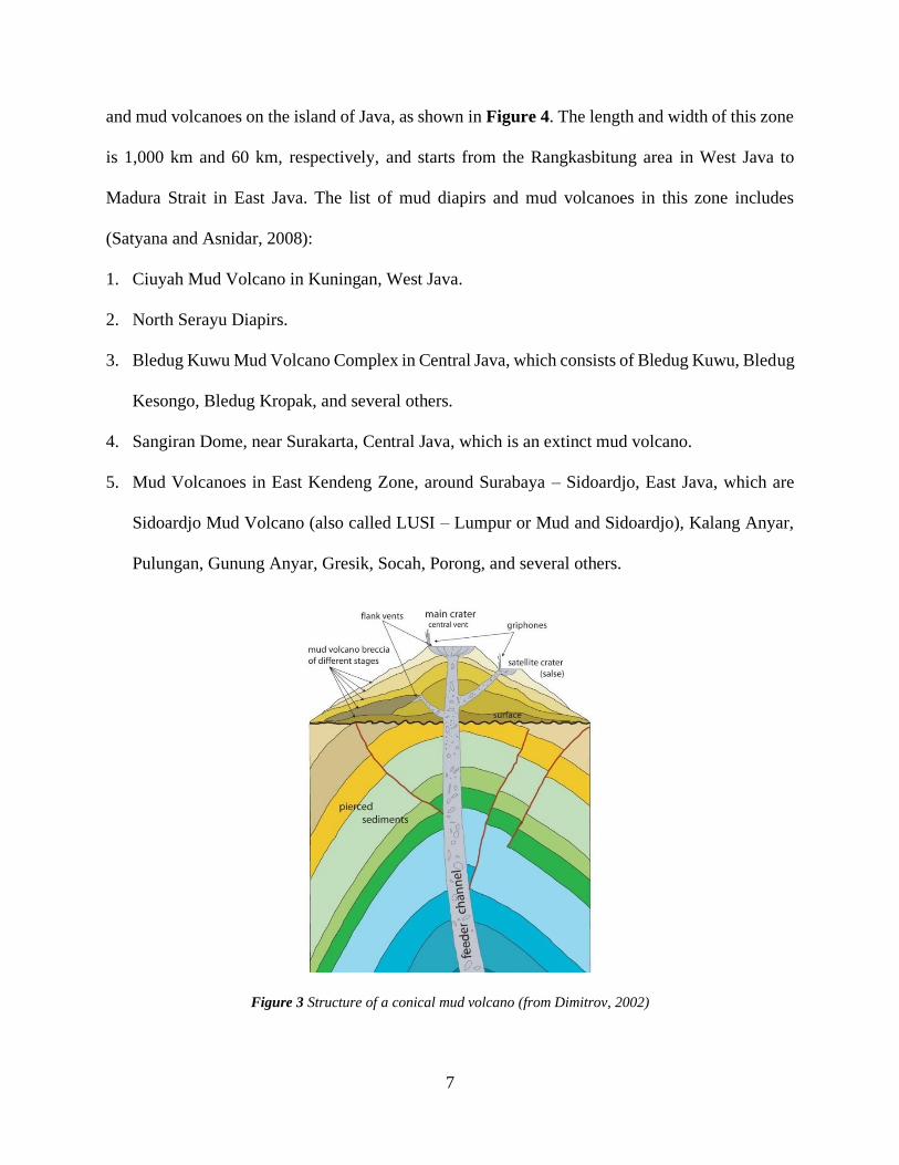
extrusion. Dimitrov (2002) studied the shape and size of mud volcanoes. He found that the general
shape of mud volcano is a conical mountain, as described in Figure 3. However, other forms such
as flat cones, domes, and calderas have also been identified. The size varies from a few meters up
to 500 m in heights and the diameter of the craters can reach up to 500 m, with the base width
extending as far as 4 km.
There are over 900 onshore and 800 offshore mud volcanoes recorded (Dimitrov, 2002). In
Indonesia, mud volcanoes can be found in Sumatra, Java, Semau, Rotti, Tanimbar, Sumba, Flores
and Papua (Williams et al., 1984; Breen et al. 1986; Silver et al. 1986; Dimitrov, 2002; Kopf,
2002). The Bogor – North Serayu – Kendeng depression zone is the main location of mud diapirs
7
and mud volcanoes on the island of Java, as shown in Figure 4. The length and width of this zone
is 1,000 km and 60 km, respectively, and starts from the Rangkasbitung area in West Java to
Madura Strait in East Java. The list of mud diapirs and mud volcanoes in this zone includes
(Satyana and Asnidar, 2008):
1. Ciuyah Mud Volcano in Kuningan, West Java.
2. North Serayu Diapirs.
3. Bledug Kuwu Mud Volcano Complex in Central Java, which consists of Bledug Kuwu, Bledug
Kesongo, Bledug Kropak, and several others.
4. Sangiran Dome, near Surakarta, Central Java, which is an extinct mud volcano.
5. Mud Volcanoes in East Kendeng Zone, around Surabaya – Sidoardjo, East Java, which are
Sidoardjo Mud Volcano (also called LUSI – Lumpur or Mud and Sidoardjo), Kalang Anyar,
Pulungan, Gunung Anyar, Gresik, Socah, Porong, and several others.
Figure 3 Structure of a conical mud volcano (from Dimitrov, 2002)
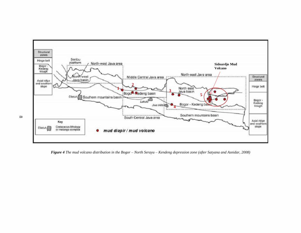
Figure 4 The mud volcano distribution in the Bogor – North Serayu – Kendeng depression zone (after Satyana and Asnidar, 2008)
1 2
3
4
5
8
Sidoardjo Mud
Volcano

9
2.2 Clay mineralogy
2.2.1 Structure of clay minerals
The term “clay material” refers to a group of phyllosilicate substance that derived from primary
materials such as quartz, feldspar, micas, etc., which have been weathered by the Earth’s surface
(Brandon and Karathanasis, 2002). The foundation of all silicate structure is a four-sided building
𝑆𝑖𝑂44− or tetrahedon, which consist of one 𝑆𝑖4+ ions at its center and four 𝑂2 ions at each apices.
The horizontal connection of tetrahedron at the three corners creates an array called tetrahedral
sheet. The other foundation is octahedron, which is an eight-sided building constructed by one
cation (i.e. aluminum or magnesium) at its center and six 𝑂2 ions surrounding the cation. A
horizontal array of multiple octahedra is called octahedral sheet. The illustration of those essential
foundations of silica structure are shown in Figure 5. Based on the formation and the number of
tetrahedral and octahedral sheet in clay minerals, we can classified the clay minerals into 3 general
group: 1:1 clay mineral, 2:1 clay mineral, and 2:1:1 clay mineral.
Figure 5 Illustration of tetrahedron and tetrahedral sheel at top and octahedron and octahedral sheet at bottom
(Aboubakr et al. 2013)
10
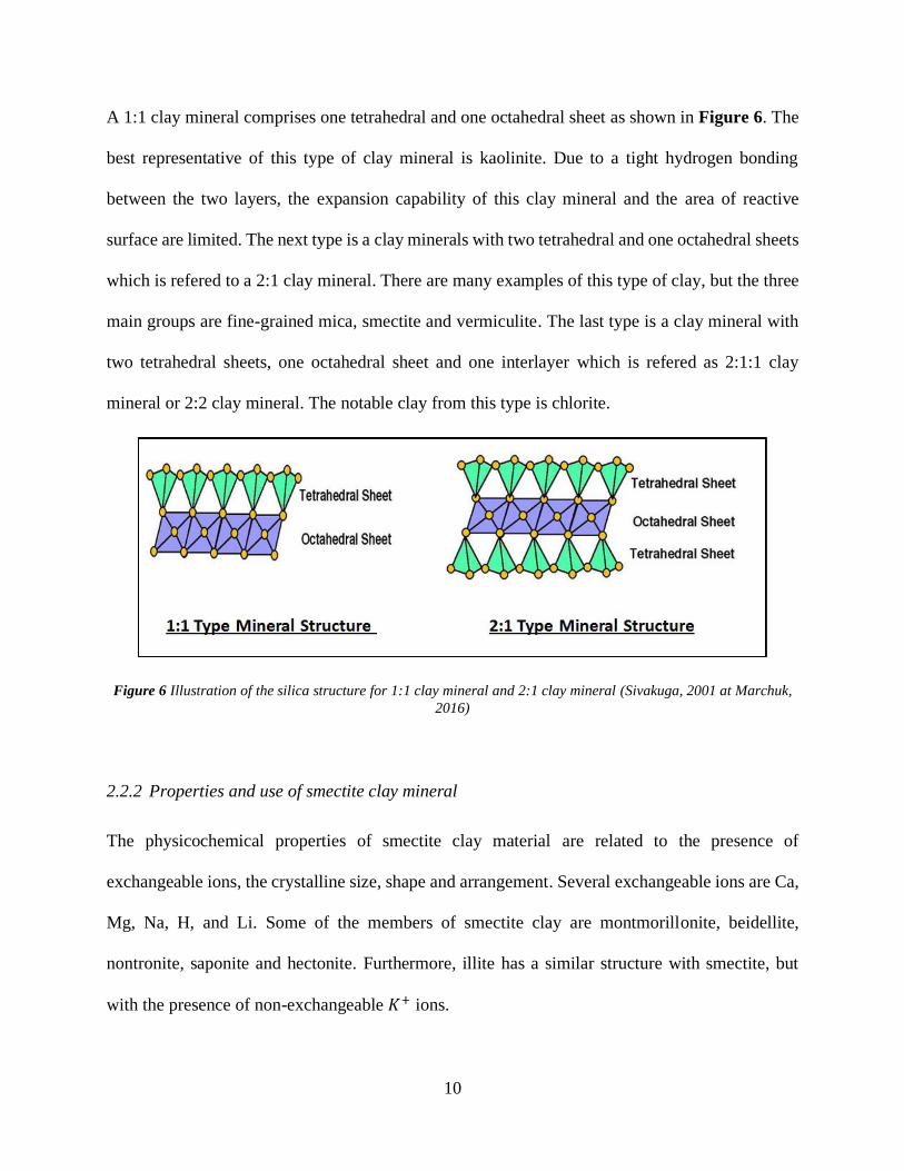
A 1:1 clay mineral comprises one tetrahedral and one octahedral sheet as shown in Figure 6. The
best representative of this type of clay mineral is kaolinite. Due to a tight hydrogen bonding
between the two layers, the expansion capability of this clay mineral and the area of reactive
surface are limited. The next type is a clay minerals with two tetrahedral and one octahedral sheets
which is refered to a 2:1 clay mineral. There are many examples of this type of clay, but the three
main groups are fine-grained mica, smectite and vermiculite. The last type is a clay mineral with
two tetrahedral sheets, one octahedral sheet and one interlayer which is refered as 2:1:1 clay
mineral or 2:2 clay mineral. The notable clay from this type is chlorite.
Figure 6 Illustration of the silica structure for 1:1 clay mineral and 2:1 clay mineral (Sivakuga, 2001 at Marchuk,
2016)
2.2.2 Properties and use of smectite clay mineral
The physicochemical properties of smectite clay material are related to the presence of
exchangeable ions, the crystalline size, shape and arrangement. Several exchangeable ions are Ca,
Mg, Na, H, and Li. Some of the members of smectite clay are montmorillonite, beidellite,
nontronite, saponite and hectonite. Furthermore, illite has a similar structure with smectite, but
with the presence of non-exchangeable 𝐾+ ions.

11
If Ca and Mg are the predominant ions, the smectite is a non-swelling clay. However, if Na or Li
are the predominant ions, the smectite has a high swelling capacity. This is because those ions help
create a layer of water in the interlamellar surface in saturated condition as presented in Figure 7.
Clay minerals with a strong swelling attribute are called active clay. In the clay industry, adding
swelling properties into clay mineral can result in an activated clay. This can be done by replacing
Ca or Mg ions with Na ion. The benefits of this are higher wet tensile strength and thermal
resistance.
Figure 7 Swelling mechanism of smectite (Aniekan et al., 2018)
When a small amount of clay mineral is added into a large amount of water, its crystal composition
separates and disperses. Furthermore, their electric potential cause the particles to repel each other.
The term for this process is called colloidal or suspension. However, when the clay mineral present
itself as a large concentration, the mixture becomes more viscous and has a high resistance to flow.
Another unique property of clay mineral is thixotropy, which indicates a decrease in viscosity

12
when subjected to applied stress. Monmorillonite, saponite and hectonite are types of smectite that
are viscous and thixotrpy because of the presence of sodium. Odom (1984) argued that smectite
clay minerals in a single deposit can have either uniform or varied viscosity due to dispersibility
and natural ion exchange.
Smectite clay minerals have been used in many processes and industries. Some notable uses are:
1. Foundry moulding sands. The metallurgy industry uses smectite in a mixture with sand and
water to make sand plastic and cohesives. They harnesses the smectite properties such as
compression strength, wet tensile strength, flowability and durability.
2. Drilling muds. The gas and oil industry uses smectite properties such as grit, viscosity, and
rheological properties to lubricare and cool the drill bit.
3. Binding agents. The food industry combines Na or Ca smectites into the pelletization process
to improve the nutrition of the animal while the iron ore industry combines the Na smectites
into the pelletization process to absorb excess water from the ore.
4. Medicine. Smectites with zinc ion and magnesium ion accelerate the absorption of bacteria
thereby accelerating wound healing (Sasaki and Yamamoto, 2017).
5. Grouting. Civil engineering practices use smectite for its viscosity, thixotropty, impermeability
and plasticity properties. This action impedes water or waste in soils and provides non-
mechanical support for excavator and construction of tunnel walls.
6. Water purification. Environmental practices employ actions to purify water from indurstrial
oils and organic waste by applying dispersion and absorptive properties of smectites (Cody
and Magauran, 1990).
13
2.3 Sidoardjo Mud Volcano
There are two theories surrounding the origins of the Sidoardjo Mud Volcano. They are: (1) it was
a natural disaster which triggered by the Yogyakarta earthquake on May 27th, 2006 (Mazzini et al.,
20017; Sawolo et al., 2009; Lupi et al., 2013); and (2) it was an underground blowout caused by
an oil drilling failure (Banjar Panji-1 exploration well) by PT Lapindo Brantas (Manga et al., 2007;
Tingay et al., 2008; Mori and Kano, 2009; Davies et al., 2007). Moreover, Mazzini et al. (2007)
suggested that the mud volcano was strongly influenced by an earthquake that took place in
Yogyakarta. His argument was based on a geochemical and field results that indicated an
earthquake did take place. Sawolo et al. (2010) stated that the underground blowout did not occur
in the exploration well based on a pressure analysis. Contrary to this theory is that the drilling
process induced hydraulic fracturing or reactivated previously inactive faults, which increased
pressure on the mud, thereby creating the conditions that led to the eruption of the mud volcano
(Davies et al., 2010; Tingay et al., 2015).
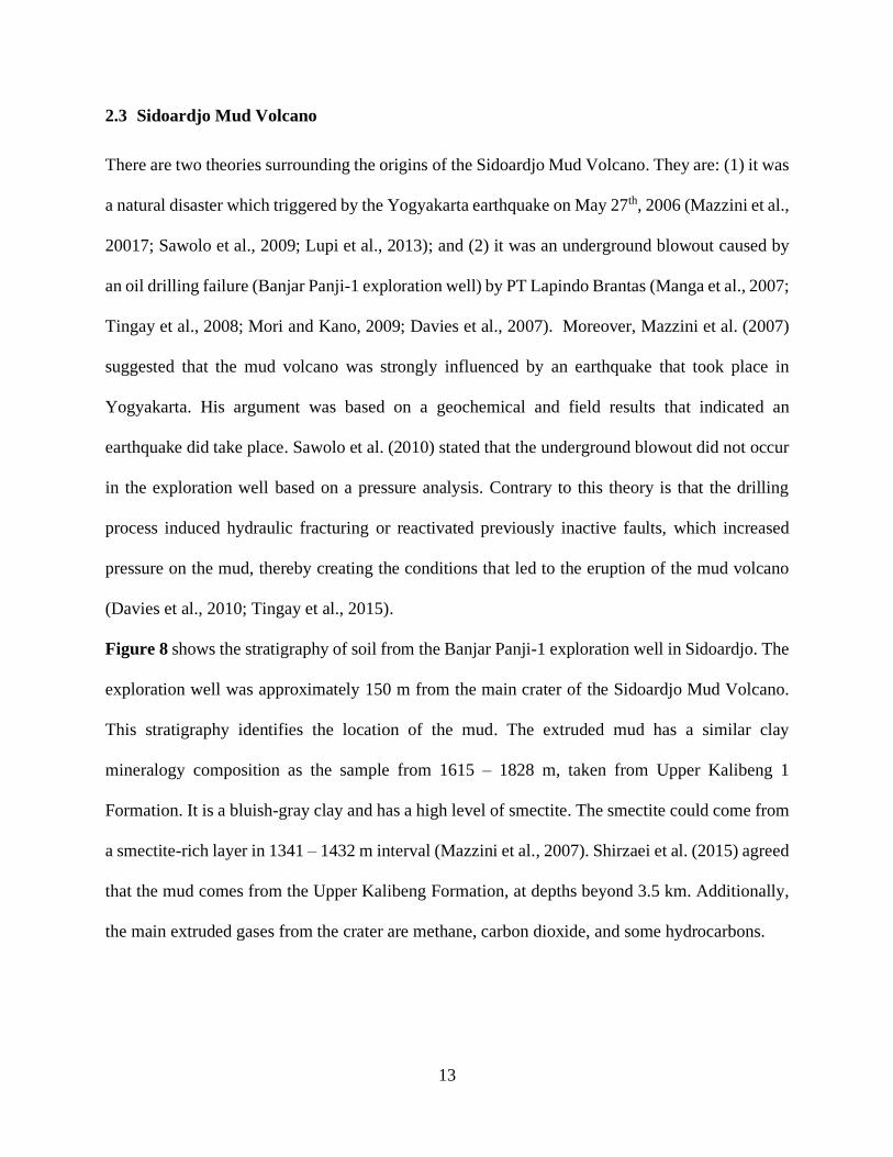
Figure 8 shows the stratigraphy of soil from the Banjar Panji-1 exploration well in Sidoardjo. The
exploration well was approximately 150 m from the main crater of the Sidoardjo Mud Volcano.
This stratigraphy identifies the location of the mud. The extruded mud has a similar clay
mineralogy composition as the sample from 1615 – 1828 m, taken from Upper Kalibeng 1
Formation. It is a bluish-gray clay and has a high level of smectite. The smectite could come from
a smectite-rich layer in 1341 – 1432 m interval (Mazzini et al., 2007). Shirzaei et al. (2015) agreed
that the mud comes from the Upper Kalibeng Formation, at depths beyond 3.5 km. Additionally,
the main extruded gases from the crater are methane, carbon dioxide, and some hydrocarbons.

14
Figure 8 Stratigraphy from Banjar Panji-1 exploration well in Sidoardjo, East Java (after Mazzini et al., 2007)
Mazzini et al. (2007) also described the evolution of the Sidoardjo Mud Volcano. He suggested
that at the beginning of the eruption, the mud volcano had an eruption rate of 5,000 m3/d which
had 60% water content. However, by December 2006, the eruption rate had peaked to 180,000
m3/d and reached 110,00 m3/d by June 2007. He went onto explain the relevance of the ellipsoid
subsiding area around the mud volcano, which had an axis of 7x4 km while some other parts had
an average subsidence rate of 1-4 cm/d. He argued that the subsidence can be caused by the weight
15
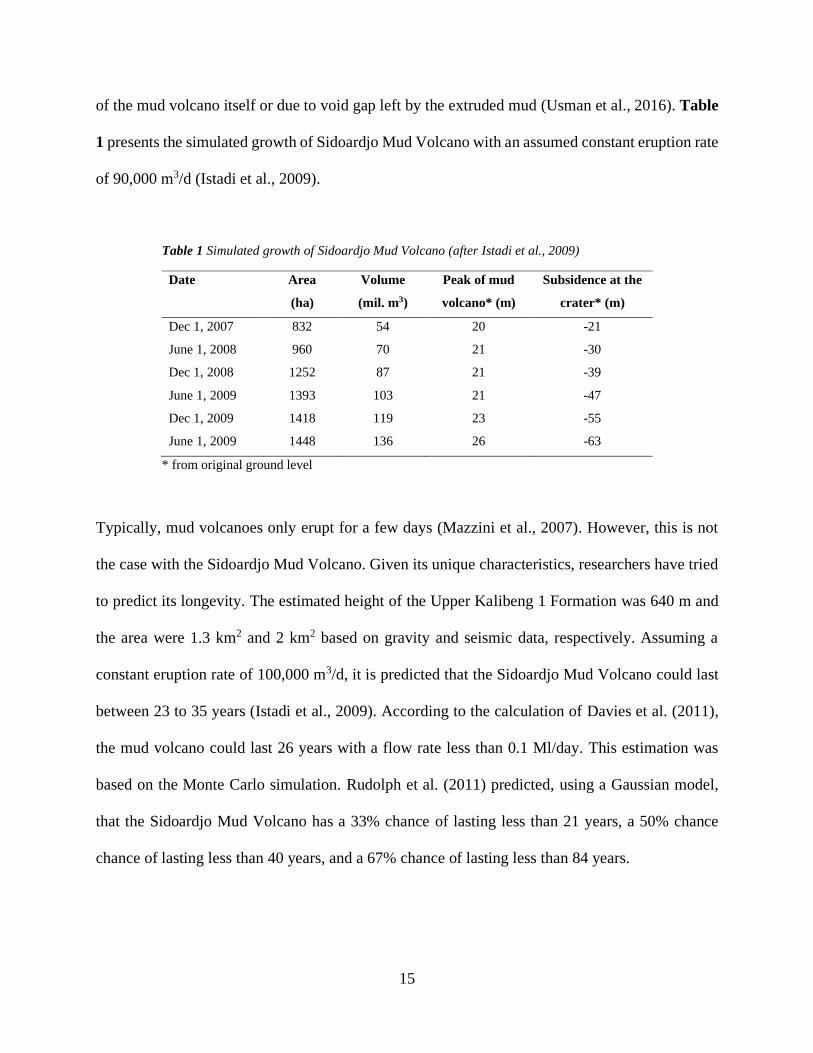
of the mud volcano itself or due to void gap left by the extruded mud (Usman et al., 2016). Table
1 presents the simulated growth of Sidoardjo Mud Volcano with an assumed constant eruption rate
of 90,000 m3/d (Istadi et al., 2009).
Table 1 Simulated growth of Sidoardjo Mud Volcano (after Istadi et al., 2009)
Date Area
(ha)
Volume
(mil. m3)
Peak of mud
volcano* (m)
Subsidence at the
crater* (m)
Dec 1, 2007 832 54 20 -21
June 1, 2008 960 70 21 -30
Dec 1, 2008 1252 87 21 -39
June 1, 2009 1393 103 21 -47
Dec 1, 2009 1418 119 23 -55
June 1, 2009 1448 136 26 -63
* from original ground level
Typically, mud volcanoes only erupt for a few days (Mazzini et al., 2007). However, this is not
the case with the Sidoardjo Mud Volcano. Given its unique characteristics, researchers have tried
to predict its longevity. The estimated height of the Upper Kalibeng 1 Formation was 640 m and
the area were 1.3 km2 and 2 km2 based on gravity and seismic data, respectively. Assuming a
constant eruption rate of 100,000 m3/d, it is predicted that the Sidoardjo Mud Volcano could last
between 23 to 35 years (Istadi et al., 2009). According to the calculation of Davies et al. (2011),
the mud volcano could last 26 years with a flow rate less than 0.1 Ml/day. This estimation was
based on the Monte Carlo simulation. Rudolph et al. (2011) predicted, using a Gaussian model,
that the Sidoardjo Mud Volcano has a 33% chance of lasting less than 21 years, a 50% chance
chance of lasting less than 40 years, and a 67% chance of lasting less than 84 years.

16
2.4 Mud Properties
2.4.1 Settling velocity
When the density of a particle is greater than the density of the surrounding fluid, it moves
downward. This movement is called settling while the speed is called settling velocity. The main
driving force behind settling velocity is the gravity force or buoyant weight, which is a function of
particle density and fluid density. The resistance force is the drag force, which is a function of
particle size and shape and the viscosity of fluid (Cheng, 1997; Pejrup and Mikkelsen, 2009).
Reichert et al. (2009) stated that the type of clay mineralogy affects the particles settling velocity.
For example, particles with high smectice clay tends to have a slower settling velocity. This is due
to dispersion. Sediment concentration also affects the settling velocity and a higher sediment
concentration leads to a slower settling velocity (Vanoni, 1962; Cheng, 1997; Shen et al., 2016).
Julien (2010) defined the settling velocity for natural particles is a function of dimensionless
particle diameter 𝑑∗:
𝜔
√(𝐺 − 1)𝑔𝑑𝑠≅
8
𝑑∗1.5((1 +
𝑑∗3
72) − 1) (1)
𝑑∗ = 𝑑𝑠 [(𝐺 − 1)𝑔
𝜐𝑚2]
13
(2)
where 𝑑𝑠 is the particle size, 𝐺 is the specific gravity of the particle, and 𝜐𝑚 is the kinematic
viscosity of the fluid.
2.4.2 Flocculation
When numbers of very fine particles, such as silt and clay, are found in a river, they tend to hold
together and form flocculated masses. This is due to electrochemical forces and high surface areas
of clay particles. There are three factors that control the flocculation processes: sediment

17
concentration, turbulence and fluid salinity. Guo et al. (2017) found that the floc size is inversely
proportional with turbulent shear, particularly with turbulent shear larger than 2-3 𝑠−1. Sutherland
(2014) investigated the effect of salinity on clay settling and found that clay flocculation occurs at
10 ppt. The effect does not increase significantly beyond 10 ppt. However, high sediment
concentration can discourage the flocculation processes of fine sediments. Flocculated settling
velocity can range from 0.15 to 0.6 mm/s and usually occurs in particles that are less than 40 𝜇𝑚
in size (Julien, 2010). Recall that clay particle has a sediment size equals or lower than 4 𝜇𝑚.
To investigate a flocculation procceses in a sediment sample, a deflocculant agent could be mixed
into a sediment mixture and then the settling velocity of the micture was recorded. If flocculation
occurs in the mixtures, the settling velocity of the mixture with the added deflocculant would be
slower than the original mixture. A deflocculant comprises 35.70 g of sodium hexametaphosphate
and 7.94 g of sodium carbonate when diluted in 1 liter of distilled water. Then 1 ml of this
deflocculant is added for every 100 ml of sample (Guy, 1969; Vanoni, 1962; Julien and
Mendelsberg, 2003).
Migniot (1989) proposed an equation to calculate the flocculated settling velocity 𝜔𝑓:
𝜔𝑓 =
250
𝑑𝑠2𝜔
(3)
where 𝑑𝑠 is the particle size in microns and 𝜔 is the settling velocity of disperse particles. To
complement Equation 4, Winterwerp (1999) provided an empirical equation to approximate the
floc size 𝑑𝑓𝑙𝑜𝑐𝑐:
𝜔𝑓 = 10𝑑𝑓𝑙𝑜𝑐𝑐1.5 (4)
where 𝜔𝑓 is in mm/s and 𝑑𝑓𝑙𝑜𝑐𝑐 is in mm.

18
2.4.3 Relationship between turbidity and sediment concentration
Turbidity is an optical property of water, which describes the ability of water to attenuate light
through scattering and absorption (McCarthy et al., 2974). The scattering process is caused by
suspended particles while absorption can be caused by dissolved matter and suspended particles
(Gippel, 1989).
To date, turbidity measurements include: Nephelometric Turbidity Units (NTU), Formazine
Nephelometric Units (FNU), Formazine Turbidity Units (FTU), and Formazine Attenuation
Units). NTU and FNU are used for turbidity measurement with nephelometric instruments and
formazine standard while FTU and FAU are used for turbidity measurements with generic
turbidimeter and formazine standard. Furthermore, the International Organization for
Standardization (2016) emphasized that NTU or FNU are more applicable for low turbidity water
such as drinking water while FAU is more applicable for a turbid water such as waste waters. Since
they use the same formazine standard, their values are the same (1 NTU = 1 FNU = 1 FTU = 1
FAU).
In civil engineering field works, turbidity can be used to estimate suspended sediment
concentration because it is hard to continuously sample sediment concentration in storm events or
in isolated sites. This approach is more accurate than using streamflow to estimate suspended
sediment concentration (Christensen et al., 2002). Some attempts at using turbidity measurements
to estimate suspended sediment concentration or the sediment load of streams have been recorded
in Jansson (1992), Lewis (1996), Minella et al. (2008), Pavanelli and Bigi (2005), Pfannkuche and
Schmidt (2003), and Riley (1998). The relationship between turbidity and suspended sediment
concentration is affected by the accuracy of the instrument. Properties of suspended sediment and
water, such as suspended particle size and shape, the color of water, composition of organic and

19
inorganic matters, and turbulence also play a role in affecting the accuracy of the result (Gippel,
1989). Therefore, calibration in laboratory or in-situ is important to develop an accurate result.
Minella et al. (2008) stressed the importance of ensuring the accuracy of laboratory and in-situ
calibration. To highlight their argument, they conducted an experiment in a small catchment areas
in Rio Grandense plateau, Rio Grande do Sul, Brazil. They installed a locally-manufactured
turbidimeter and Parshall flume to measure the turbidity and discharge, respectively, for 8 storm
events between July 2004 and May 2005. In-situ calibration was done by collecting 458 suspended
sediment samples with USDH-48 near the turbidimeter. They then measured the concentration
through evaporation and paired it with the corresponding turbidity and discharge. Laboratory
calibration was done by collecting different soils that represented the suspended sediment in the
river, sieving it for the fine particles, weighing it, and finally diluting it in 1 liter river water. Then
they recorded the concentration and turbidity of the samples. Half of the in-situ collected samples
were used to derive the regression equation for turbidity as the independent variable and suspended
sediment concentration as the dependent variable. The other half of the in-situ collected samples
were used to determine an error of the regression equation. The error 𝑒 was calculated by using
the following equation:
𝑒 = √(𝑆𝑆𝐶𝑐𝑎𝑙𝑐 − 𝑆𝑆𝐶𝑚𝑒𝑎𝑠)2
𝑛 − 1 (5)
where SSCcalc is the predicted or calculated suspended sediment concentration from turbidity
value, SSCmeas is the observed or measured suspended sediment concentration, and 𝑛 is the number
of samples. The error between in-situ and laboratory calibration were ±122 mg/l and -601 mg/l,
respectively, which indicates that the in-situ calibration is superior to the laboratory calibration.
Figure 9 supports these results particularly where the predicted suspended sediment

20
concentrations were similar to the observed concentration with some underestimated values at high
concentration for in-situ calibration. On the other hand, the predicted concentration was
overestimated for laboratory calibration. The dilution effect for turbid water, which was for
samples beyond the maximum limit of the instrument, can cause further error in laboratory
calibration (Pavanelli and Bigi, 2005).
Figure 9 Comparison of the observed and predicted suspended sediment concentration for (a) in-situ calibration,
and (b) laboratory calibration (after Minella et al., 2008)
In laboratory experiments, Holliday et al. (2003) found that turbidity measurements can be used
to accurately estimate the suspended sediment concentration. However, the presence of sand or
larger particles can cause an underestimated or inaccurate estimations (Riley, 1998). These studies
followed on work conducted by Foster et al. (1992) on the effects of particle size on the relationship
between turbidity and sediment concentration in Midland UK as shown in Figure 10.
Table 2 and Figure 11 summarize the relationship between turbidity in NTU, FTU, or TUR and
suspended sediment concentration (SSC) or total suspended sediment (TSS) or suspended
a) b)
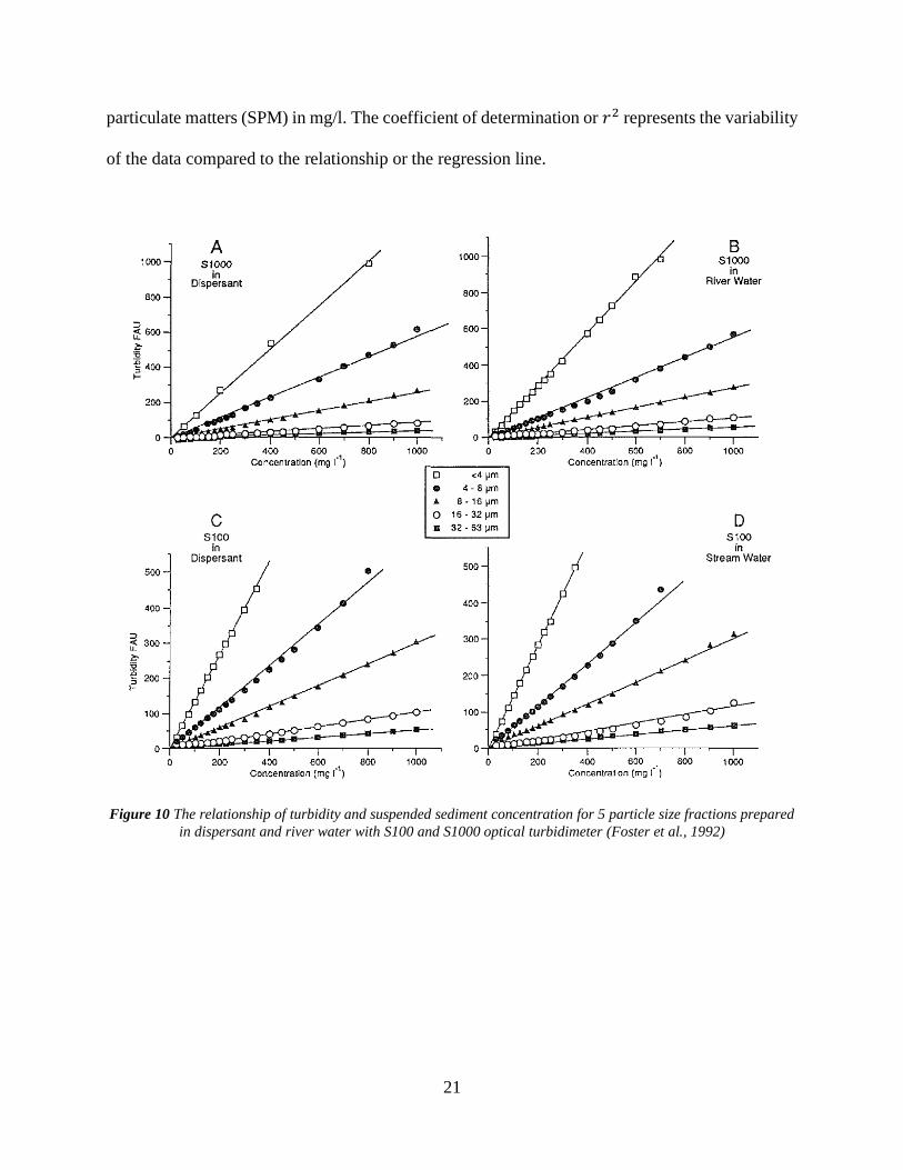
21
particulate matters (SPM) in mg/l. The coefficient of determination or 𝑟2 represents the variability
of the data compared to the relationship or the regression line.
Figure 10 The relationship of turbidity and suspended sediment concentration for 5 particle size fractions prepared
in dispersant and river water with S100 and S1000 optical turbidimeter (Foster et al., 1992)

22
Table 2 Summary of the relationship between turbidity and sediment concentration from previous studies
Location and Reference Relationship 𝑹𝟐 Remarks
1 Doce River, Brazil by Palu and Julien
(2019)
𝑁𝑇𝑈 = 2 × 𝐶 0.98
2 Cecil Ap soil by Holliday et al. (2003) 𝑁𝑇𝑈 = 0.4833 × 𝑇𝑆𝑆1.012 0.9987 Whole soil
𝑁𝑇𝑈 = 1.0283 × 𝑇𝑆𝑆1.0282 0.9991 Silt + clay
𝑁𝑇𝑈 = 0.7733 × 𝑇𝑆𝑆0.9336 0.9996 Clay
3 N’djili Basin, Congo by Ndolo Goy
(2015)
log 𝑇𝑆𝑆 = 0.9269 × log𝑁𝑇𝑈 + 0.613 0.9955 2005
log 𝑇𝑆𝑆 = 0.9327 × log𝑁𝑇𝑈 + 0.6306 0.9838 2013
4 Ranger Uranium Mine, Australia by Riley
(1998)
𝑆𝑒𝑑 𝐶𝑜𝑛 = 0.6 × 10⁻⁶ × 𝑇𝑢𝑟𝑏1.166 0.58
5 Elbe River, Germany by Pfannkuche and
Schmidt (2003)
𝑆𝑃𝑀 = 0.695 × 𝑁𝑇𝑈 + 15.20 0.6
6 Sillaro Torrent, Italy by Pavanelli and Bigi
(2005)
𝑆𝑆𝐶 = 0.65 × 10⁻⁶ × 𝑁𝑇𝑈 + 0.00278 0.79 Fresh sample
𝑆𝑆𝐶 = 0.60 × 10⁻⁶ × 𝑁𝑇𝑈 + 0.00142 0.98 1 month old sample
7 Avorezinha, Brazil by Minella et al.
(2008)
𝑆𝑆𝐶 = 0.098 × 𝑇𝑈𝑅2.313 0.86 In situ
𝑆𝑆𝐶 = 0.569 × 𝑇𝑈𝑅2.039 0.807 Laboratory
8 Geeburg Creek by Gippel (1989) 𝐹𝑇𝑈 = 1.22 × 𝑇𝑆𝑆 − 9.70 0.858 Corrected for color
9 Singapore by Daphne et al. (2011) 𝑇𝑆𝑆 = 0.7992 × 𝑁𝑇𝑈 0.8009 For sample with
𝑇𝑆𝑆 < 80 𝑚𝑔/𝑙
23
Figure 11 The relationship between turbidity and sediment concentration from previous studies
2.4.4 Properties of Sidoardjo mud
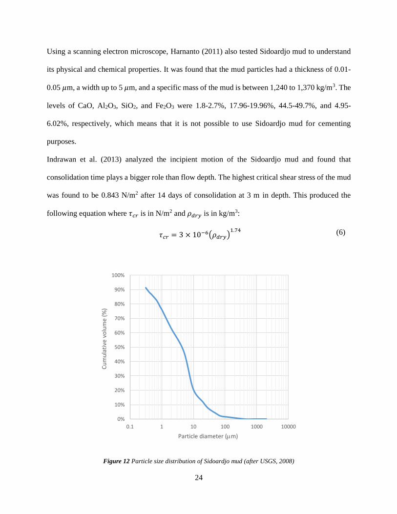
It is important to understand the characteristics of the mud from the mud volcano. A preliminary
study about the characteristics of Sidoardjo mud was conducted by Plumlee et al. (2008). They
found that the mud contained mostly clay minerals (73.6%) followed by quartz (8.3%) and feldspar
(5.6%). Smectite and illite are the dominant clay minerals. Results from the particle size analysis
are shown in Figure 12. Mostly particles are finer than 10 𝜇m.
24
Using a scanning electron microscope, Harnanto (2011) also tested Sidoardjo mud to understand
its physical and chemical properties. It was found that the mud particles had a thickness of 0.01-
0.05 𝜇m, a width up to 5 𝜇m, and a specific mass of the mud is between 1,240 to 1,370 kg/m3. The
levels of CaO, Al2O3, SiO2, and Fe2O3 were 1.8-2.7%, 17.96-19.96%, 44.5-49.7%, and 4.95-
6.02%, respectively, which means that it is not possible to use Sidoardjo mud for cementing
purposes.
Indrawan et al. (2013) analyzed the incipient motion of the Sidoardjo mud and found that
consolidation time plays a bigger role than flow depth. The highest critical shear stress of the mud
was found to be 0.843 N/m2 after 14 days of consolidation at 3 m in depth. This produced the
following equation where 𝜏𝑐𝑟 is in N/m2 and 𝜌𝑑𝑟𝑦 is in kg/m3:
𝜏𝑐𝑟 = 3 × 10⁻⁶(𝜌𝑑𝑟𝑦)
1.74 (6)
Figure 12 Particle size distribution of Sidoardjo mud (after USGS, 2008)
0%
10%
20%
30%
40%
50%
60%
70%
80%
90%
100%
0.1 1 10 100 1000 10000
Cu
mu
lati
ve v
olu
me
(%)
Particle diameter (m)

25
2.5 Sediment Transport in Rivers
2.5.1 Mixing processes
When sediments or contaminants are discharged into a river, they undergo three mixing stages
(Fischer et al., 1979; Jung et al., 2019). The first stage is a mixing process controlled by momentum
and buoyancy, the second stage is lateral mixing caused by the turbulence in the river, while the
third stage is longitudinal dispersion which diminishes the longitudinal concentration gradient.
The mixing processes, particularly the second stage, can be analyze using the advection-diffusion
equation The complete three-dimensional advection-diffusion equation is:
𝜕𝐶
𝜕𝑡+ 𝑢
𝜕𝐶
𝜕𝑥+ 𝑣
𝜕𝐶
𝜕𝑦+ 𝑤
𝜕𝐶
𝜕𝑧= �̇� + (𝐷 + 𝜀𝑥)
𝜕2𝐶
𝜕𝑥2+ (𝐷 + 𝜀𝑦)
𝜕2𝐶
𝜕𝑦2+ (𝐷 + 𝜀𝑧)
𝜕2𝐶
𝜕𝑧2
(7)
where 𝐶 represents the mass concentration, 𝐷 is the molecular diffusion, and 𝜀 represents the
turbulent mixing coefficient. Phase change, �̇�, is applied on nonconservative substance which
could undergoes the internal mass change such as sedimentation, decay or chemical reaction
(Julien, 2010). The molecular diffusion 𝐷 is negligible compared to the turbulent mixing in rivers.
In this research, the author would replace the x, y, and z coordinates correspond to the longitudinal,
transversal and vertical direction, respectively (𝜀𝑥 = 𝐾𝑑, 𝜀𝑦 = 𝜀𝑡, 𝑎𝑛𝑑 𝜀𝑧 = 𝜀𝑣).
Fischer et al. (1979) proposed empirical functions for the longitudinal dispersion coefficient,
vertical and transversal mixing coefficient, 𝐾𝑑, 𝜀𝑣 and 𝜀𝑡, respectively for natural channels in m2/s:
𝐾𝑑 ≅ 0.011
𝑈2𝑊2
ℎ𝑢∗ 𝜀𝑣 ≅ 0.067 ℎ𝑢∗ 𝜀𝑡 ≅ 0.6 ℎ𝑢∗
(8)
where 𝑈 is the mean flow velocity, 𝑊 is the channel width, ℎ is flow depth and 𝑢∗ is the shear
velocity on average equals to √𝑔ℎ𝑆 with 𝑔 is the gravitational acceleration and 𝑆 is the energy
advective Diffusion and turbulent mixing phase
change mass
change

26
slope. The use of dispersion coefficient is more appropriate than turbulent mixing coefficient
because the mass motion, due to molecular diffusion and shear flow (advective motion), is additive
and it is often hard to differentiate (Aris, 1956).
The first-order approximation of time and length scales of longitudinal dispersion, vertical and
transversal mixing are:
𝑋𝑑 =
(500ℎ𝑢∗)
𝑈 𝑋𝑣 =
ℎ𝑈
0.1𝑢∗ 𝑋𝑡 = 𝑡𝑡𝑉 =
𝑊2𝑈
ℎ𝑢∗ (9)
𝑡𝑑 ≅
𝑋𝑑2
500ℎ𝑢∗ 𝑡𝑣 ≅
ℎ
0.1𝑢∗ 𝑡𝑡 =
𝑊2
ℎ𝑢∗ (10)
The three-dimensional advection diffusion equation can be simplified in the case of straight
channels. Assume that the most dominant process occurs in the longitudinal 𝑥 direction, which for
steady point sources implies 𝑣 = 𝑤 ≅ 0 𝑎𝑛𝑑 𝐾𝑑 ≅ 0. Turbulent flow in natural channels lets us
to neglect the molecular diffusion, and after vertical mixing complete, we can assume 𝜀𝑣 ≅ 0.
For a nonconservative substance, the term �̇� in the advection-diffusion equation will not be zero
This is due to internal mass change such as settling or decay. For example, in stagnant fluid, the
advection-diffusion equation and the solution are:
𝜕𝐶
𝜕𝑡= −𝑘𝐶 (11)
𝐶𝑖 = 𝐶0𝑒−𝑘𝑡 (12)
𝐶𝑖 = 𝐶0𝑖𝑒
−𝑋𝜔𝑖ℎ𝑈 (13)
where 𝑘 is the decay or settling rate, 𝐶𝑜,𝑖 is the initial or upstream sediment concentration of
fraction 𝑖, 𝐶𝑖 is the downstream sediment concentration of fraction 𝑖, 𝑋 is the distance, ℎ is flow
depth, 𝑈 is the flow velocity, and 𝜔𝑖 is the settling velocity of the fraction 𝑖. The value of settling
27
rate 𝑘 for suspended sediment can be defined as 𝑘 = 𝜔/ℎ where 𝜔 is the fall velocity and ℎ is the
flow depth. Meanwhile, the time 𝑡 can be defined as 𝑋/𝑈.
The analytical solution of one-dimensional advection-diffusion equation with settling for
instantaneous mass injection is:
𝐶(𝑥, 𝑡) =
𝑚𝑝
2√𝜋𝐾𝑑𝑡𝑒−(𝑥−𝑈𝑡)2
4𝐾𝑑𝑡−𝑘𝑡
(14)
The analytical solution proposed by O’Loughlin and Bowmer (1975) for infinite duration of
continuous mass injection was:
𝐶(𝑥, 𝑡) =
𝐶02[𝑒
𝑈𝑥2𝐾𝑑
(1−Γ)𝑒𝑟𝑓𝑐 (
𝑥 − 𝑈𝑡Γ
2√𝐾𝑑𝑡) + 𝑒
𝑈𝑥2𝐾𝑑
(1+Γ)𝑒𝑟𝑓𝑐 (
𝑥 + 𝑈𝑡Γ
2√𝐾𝑑𝑡)] (15)
Γ = √1 + 4𝜂 ; 𝜂 =
𝑘𝐾𝑑𝑈2 (16)
In case of a mass injection of finite duration 𝜏 into a channel system, the previous analytical
solution (Chapra, 1997; Julien, 2018; Palu, 2019) can be used while the mass is being injected
(𝑡 < 𝜏). For 𝑡 > 𝜏, the analytical solution for sediment concentration 𝐶 is:
𝐶(𝑥, 𝑡) =
𝐶02{𝑒
𝑈𝑥2𝐾𝑑
(1−Γ)[𝑒𝑟𝑓𝑐 (
𝑥 − 𝑈𝑡Γ
2√𝐾𝑑𝑡) − 𝑒𝑟𝑓𝑐 (
𝑥 − 𝑈(𝑡 − 𝜏)Γ
2√𝐾𝑑(𝑡 − 𝜏))]
+ [𝑒𝑈𝑥2𝐾𝑑
(1+Γ)𝑒𝑟𝑓𝑐 (
𝑥 + 𝑈𝑡Γ
2√𝐾𝑑𝑡)
− 𝑒𝑈𝑥2𝐾𝑑
(1+Γ)𝑒𝑟𝑓𝑐 (
𝑥 + 𝑈(𝑡 − 𝜏)Γ
2√𝐾𝑑(𝑡 − 𝜏))]}
(17)
Γ = √1 + 4𝜂 ; 𝜂 =
𝑘𝐾𝑑𝑈2
(18)
where 𝐶0 is the initial sediment concentration, 𝑈 is the mean flow velocity, 𝐾𝑑 is the longitudinal
dispersion coefficient, and 𝑘 is the settling rate.

28
For a conservative substance (assuming no settling of the fine volcano mud), the phase change �̇�
is assumed equal to 0 (Julien 2018). We can further simplify the advection-diffusion equation to:
𝜕𝐶
𝜕𝑡+ 𝑈
𝜕𝐶
𝜕𝑥= 𝜀𝑡
𝜕2𝐶
𝜕𝑦2 (19)
The analytical solution of the simplified advection diffusion equation for infinitely wide channel
due to continuous mass flux injection �̇� is (Fischer et al., 1979):
𝐶(𝑥, 𝑦) = [
�̇�
ℎ√4𝜋𝜀𝑡𝑥𝑈] 𝑒
−𝑦2𝑈4𝜀𝑡𝑥 (20)
Most rivers cannot be assumed as an infinitely wide channel. Additional consideration due to
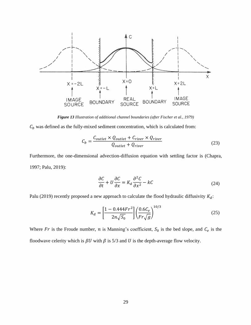
channel boundaries should be added with the method of superposition as illustrated in Figure 13.
If the sediment source located at 𝑋 = 0 and both banks located at 𝑋 = ±𝐿, by adding imaginary
sources at 𝑋 = ±2𝐿,±4𝐿, ±6𝐿,… ,±𝑛𝐿, a zero concentration gradient at the boundaries could be
achieved (or 𝜕𝐶/𝜕𝑦 = 0 at 𝑦 = 0 and 𝑦 = 𝑊). Assume 𝑦0 is the location of mass injection. The
solution of the simplified advection diffusion equation after considering the boundaries of the
channels is:
𝐶
𝐶𝑏=
1
√4𝜋𝑥′ ∑ {exp [−
(𝑦′ − 2𝑛 − 𝑦0′)2
4𝑥′] + exp [−
(𝑦′ − 2𝑛 + 𝑦0′)2
4𝑥′]}
∞
𝑛=−∞
(21)
𝐶𝑏 =
�̇�
𝑈ℎ𝑊 𝑥′ =
𝑥𝜀𝑡𝑈𝑊2
𝑦′ =𝑦
𝑊 𝑦0
′ =𝑦0𝑊
(22)
29
Figure 13 Illustration of additional channel boundaries (after Fischer et al., 1979)
𝐶𝑏 was defined as the fully-mixed sediment concentration, which is calculated from:
𝐶𝑏 =
𝐶𝑜𝑢𝑡𝑙𝑒𝑡 × 𝑄𝑜𝑢𝑡𝑙𝑒𝑡 + 𝐶𝑟𝑖𝑣𝑒𝑟 × 𝑄𝑟𝑖𝑣𝑒𝑟𝑄𝑜𝑢𝑡𝑙𝑒𝑡 + 𝑄𝑟𝑖𝑣𝑒𝑟
(23)
Furthermore, the one-dimensional advection-diffusion equation with settling factor is (Chapra,
1997; Palu, 2019):
𝜕𝐶
𝜕𝑡+ 𝑈
𝜕𝐶
𝜕𝑥= 𝐾𝑑
𝜕2𝐶
𝜕𝑥2− 𝑘𝐶 (24)
Palu (2019) recently proposed a new approach to calculate the flood hydraulic diffusivity 𝐾𝑑:
𝐾𝑑 = [
1 − 0.444𝐹𝑟2
2𝑛√𝑆0] (0.6𝐶𝑒
𝐹𝑟√𝑔)
10/3
(25)
Where 𝐹𝑟 is the Froude number, 𝑛 is Manning’s coefficient, 𝑆0 is the bed slope, and 𝐶𝑒 is the
floodwave celerity which is 𝛽𝑈 with 𝛽 is 5/3 and 𝑈 is the depth-average flow velocity.

30
The value of Manning’s coefficient 𝑛 had been studied previously (Chow, 1959). It can be
determined by using Manning’s equation such as,
𝑈 =1
𝑛𝑅23𝑆𝑓
12
where 𝑈 is the depth-average flow velocity, 𝑅 is the hydraulic radius, and 𝑆𝑓 is the friction slope
of the flow. Another method to determine the Manning’s coefficient 𝑛 is using Table 3 to choose
a value of 𝑛 for an appropriate description of the river or channel.
Table 3 The value of Manning’s coefficient (after Brunner, 2016)
Type of Channel Minimum Normal Maximum
A. Natural Streams – Main Channels
a. Clean, straight full, no rifts or deep pools
b. Same as above, but more stones and weeds
c. Clean, winding, some pools and shoals
d. Same as above, but some weeds and stones
e. Same as above lower stages, more ineffective slopes
and sections
f. Same as “d” but more stones
g. Sluggish reaches, weedy, deep pools
h. Very weedy reaches, deep pools, or floodwats with
heavy stands of timber and brush
0.025
0.030
0.033
0.035
0.040
0.045
0.050
0.070
0.030
0.035
0.040
0.045
0.048
0.050
0.070
0.100
0.033
0.040
0.045
0.050
0.055
0.060
0.080
0.150
B. Excavated or Dredged Channel
1. Earth, straight and uniform
a. clean, recently completed
b. clean, after weathering
c. gravel, uniform section, clean
d. with short grass, few weeds
2. Earth, winding and sluggish
a. No vegetation
b. Grass, some weeds
c. Dense weeds or aquatic plants in deep channels
d. Earth bottom and rubble side
e. Stony bottom and weedy banks
f. Cooble bottom and clean sides
0.016
0.018
0.022
0.022
0.023
0.025
0.030
0.028
0.025
0.030
0.018
0.022
0.025
0.027
0.025
0.030
0.035
0.030
0.035
0.040
0.020
0.025
0.03
0.033
0.030
0.033
0.040
0.035
0.040
0.050

31
2.5.2 Suspended sediment transport
One of the most important parameters in sediment transport is the Rouse number, 𝑅𝑜. This
parameter, proposed by Rouse (1937), defines the ratio of downward particle movement due to
settling and upward particle movement due to turbulent mixing (Ettema, 2006). The sediment
concentration C at point z can be determine from the Rouse equation:
𝐶
𝐶𝑎= (
ℎ − 𝑧
ℎ 𝑎
ℎ − 𝑎)𝑅𝑜
(26)
𝑅𝑜 =𝜔
𝛽𝑠𝜅𝑢∗
(27)
where 𝐶𝑎 is reference sediment concentration at reference point a from bed level, 𝜔 is the settling
velocity of particles, 𝛽𝑠 is the momentum coefficient which is assumed to equal 1 for uniform flow
(Chow, 1959), 𝜅 is the von Kármán constant which equals to 0.4, and 𝑢∗ is the shear velocity.
The Rouse equation is usually employed to construct a sediment concentration distribution or
vertical sediment concentration profile. Researchers such as Hunt (1954), Tanaka-Sugimoto
(1958), Ni and Wang (1991), Mazumder and Ghoshal (2006), and Xhu et al. (2017) have used this
equation to estimate the sediment concentration profile. The latter used empirical model while the
others used mathematical model such as the diffusion equation. Kineke and Sternberg (1989)
suggested that data obtained from in-situ methods, through a microcamera to capture the actual
floc size or settling cylinder to measure the settling velocity, works better than data estimated from
the particle size distribution of sediment sample. This is particularly the case when predicting the
sediment concentration distribution.
Akalin (2002) tried to determine the Rouse number by plotting the suspended sediment
concentration versus (ℎ − 𝑧)/𝑧 as shown in Figure 14. Parameter (ℎ − 𝑧)/𝑧 is the ratio of the
distance from the top and distance from the bottom of the point of interest. He used suspended

32
sediment data collected from the Lower Mississippi River and found that the Rouse number is the
slope of the power function of the suspended sediment soncentration. He also found that the water
temperature has an inverse effect on the Rouse number due to the change of water viscosity.
Figure 14 Proposed method to determine Rouse number (after Akalin, 2002)
Julien (2010) classified the mode of sediment transport in rivers based on the Rouse number, as
shown in Table 4. The bed load is a mode of sediment transport which is dominated by a coarser
sediment load at a thin layer near the bed level. The bed load condition is indicated by a high Rouse
number (𝑅𝑜 > 5) which means that the settling velocity 𝜔 is much higher than the upward
movement due to turbulence. The bed load was studied by Meyer-Peter and Muller (1948), van
Rijn (1984a), and Kociuba (2017). On the other hand, a suspended load is dominated by fine
sediment in suspension, as put forward by van Rijn (1984b), Yang et al. (1996), Shah-Fairbank et
al. (2011), and Vercruysse at al. (2017). In the case of suspended load, the settling velocity of the
y = 63.327x0.6536
R² = 0.6086
1
10
100
1000
0.1 1 10 100
Susp
end
ed S
edim
ent
Co
nce
ntr
atio
n, C
(p
pm
)
(h-z)/z

33
particles and the Rouse number are small (𝑅𝑜 < 1.25). This is also the view of Allen et al. (1979)
and Shi (2010) who studied the tidal effects to the transport of suspended sediment. Between the
two modes of sediment transport is a mixed load which both bed load and suspended load
contribute to the total load.
Table 4 Classification of the mode of sediment transport
Ro 𝒖∗/𝝎 Mode of Sediment Transport
> 𝟏𝟐. 𝟓 < 0.2 No motion
≅ 𝟏𝟐. 𝟓 ≅ 0.2 Incipient motion
𝟏𝟐. 𝟓 − 𝟓 0.2 − 0.5 Bed load
𝟓 − 𝟏. 𝟐𝟓 0.5 − 2 Mixed load
< 𝟏. 𝟐𝟓 > 2 Suspended load
The sediment load by size fraction can be calculated by using the following equation (Julien,
2010),
𝑞𝑏 =∑∆𝑝𝑖𝑞𝑏𝑖 (28)
Where ∆𝑝𝑖 is the relative weight of fraction i of the sediment and 𝑞𝑏𝑖 is the unit sediment discharge
for fraction i.
There are field measurement techniques to analyzed suspended sediment (Hamilton et al., 1999;
Wren et al., 2000; Julien, 2010; Armijos et al., 2015), such as:
1. Water sampling methods; a direct measurement of suspended sediment concentration
employed by taking water (or sample) from the site. This method includes instantaneous
sampling, point sampling and depth-integrated sampling.
34
2. Optical methods; an indirect measurement where instruments, such as nephelometer and
transmissometers, record light backscatters or attenuation.
3. Acoustic Methods; another indirect measurement where instruments capture the
backscatter noises of particles.
Armijos et al. (2015) proposed additional field measurement protocols such as separation of the
turbidity measurement and the Rouse profile for fine and coarse sediment. He argued that
particularly for coarse sediment, at least one measurement of turbidity and sample for
granulometry at less than 1 m from bed level are needed. The recorded Rouse number for fine
sediment ranged from 0.01-0.03 while for coarse sediment ranged from 0.25-0.6.
2.5.3 Suspended sediment transport in Porong River
Hermawan (2012) studied the discharge of the Porong River, which was used to transport mud
into the estuary. HEC-RAS was used to simulate the sediment transport of the Porong River for
several discharge scenarios ranging from 10 to 600 m3/s. Using the Toffaleti transport function, he
found that a minimum discharge of 200 m3/s was required to transport the mud mixture to the
Madura Strait. Based on the incipient motion analysis, at least 126 m3/s was needed to flush the
bed of the Porong River and 270 m3/s was needed to flush away all the mud, including the settled
mud, to the estuary of the Porong River (Indrawan et al., 2013).
Degradation was recorded at several locations along the Porong River, particularly between the
upstream and the middle reach, which was about 4 m between October 2008 to February 2009. It
was caused by a much lower sediment inflow from the upstream region than the transport capacity
of the Porong River (Harnanto, 2011). Degradation mainly occurs during the wet season from
November to April and aggradation occurs from June to November. The degradation and
aggradation did not decrease the flood capacity of the Porong River because the deposition material

35
could be easily flushed away by the flood during the wet season (Kure et al., 2014). Hernawan and
Budiono (2013), however, observed sediment sorting for each size fraction. Sand fraction was
found along the thalweg of Porong River while silts and clays were found near the bank of the
Porong River. They concluded that while the mud was found in the Porong River estuary, no mud
from the mud volcano was found in the outskirt of the Porong River estuary. The deposition of
sediment at the mouth of the Porong River was caused by the confluence of a high river discharge
and a high tidal and monsoon-induced flow, which hindered the transport processes (Hoekstra,
1988). This accounted for the final location of the mud is on flat slope areas at a depth of 20-60 m
in Madura Strait (Usman et al., 2016).
Several studies have been conducted to estimate the concentration of pollutants (for example the
suspended sediment concentration) in the Porong River and its estuary. Jennerjahn et al. (2013)
compared the level of contaminants in the Porong River and its estuary before and after the
eruption. They collected data from 1991-1998. The research team conducted another assessment
in 2002-2003 and another one in 2008. In 2008, the TSS had increased by 1 to 2 orders of
magnitude during the dry and wet seasons compared to the 1991-1998 and 2002-2003. The
maximum TSS during the dry and wet seasons of 2008 are 967 mg/l and 2,299 mg/l, respectively.
This was observed 9 km from the mouth of the Porong River.
The modeling of contaminants along the Porong River after the Sidoardjo Mud Volcano was
conducted by Suntoyo et al. (2015), using the Mike 21 Hydrodynamics and Ecolab module. The
model had 10 simulation days with 240 time steps. This simulation was validated with the
measurement data from the downstream end of the Porong River. The maximum TSS from the
simulation was 300 mg/l, which is lower than the water quality standard.
36
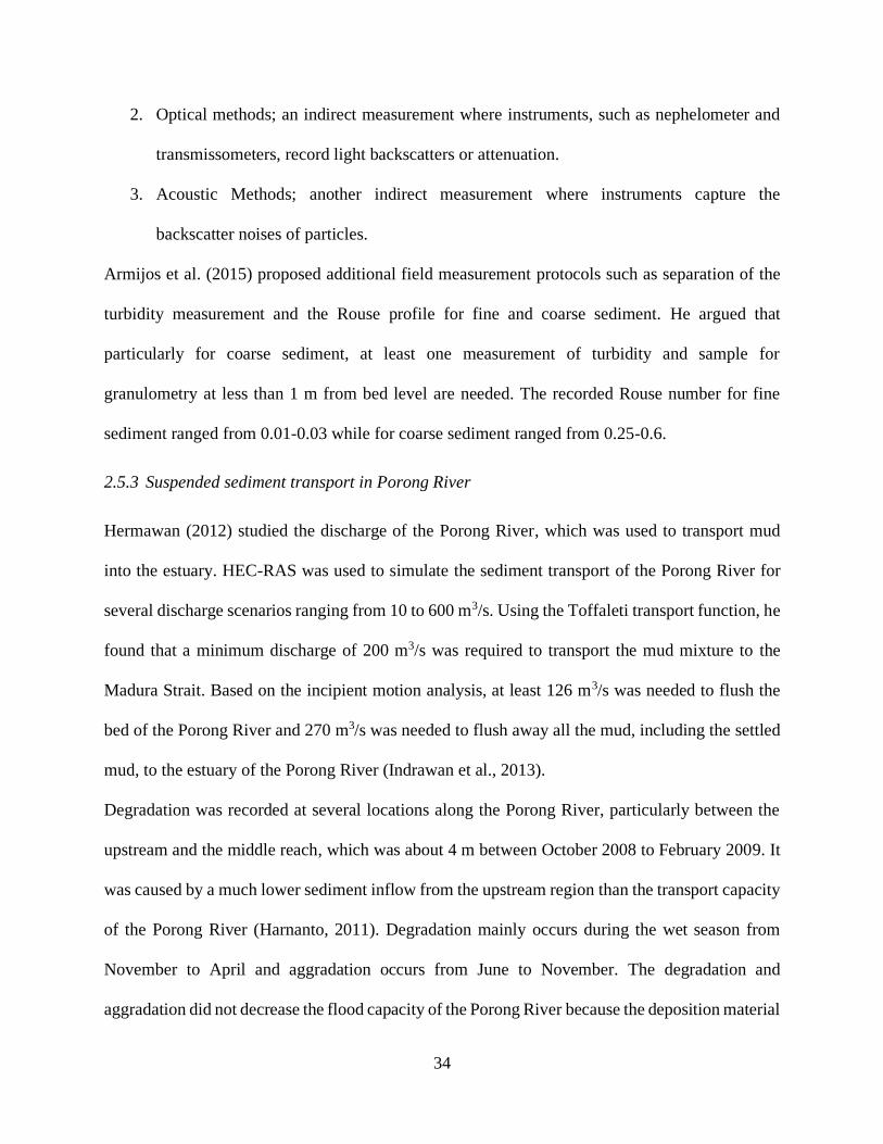
Based on the imagery from ASTER 2005-2008, Landsat5 TM 1994, and Landsat 7 ETM+ 2003,
the sediment concentration (TSS) ranged between 50-100 mg/l in 1994-2005 and 100-150 mg/l in
2006. It increased to >200 mg/l in 2007-2008 as a result of the mud volcano (Pahlevi and Wiweka,
2010). Another estimation method for TSS was proposed using the Sentinel-2 imagery (Bioresita
et al., 2018) where the Laili algorithm for Landsat imagery was adapted. The imagery from January
12, 2016 as shown in Figure 15 denotes a black area at the left side which is masked land and the
gray area is the coastal area. To validated the algorithm, 9 in-situ data were collected on April 20,
2016 (marked with plus sign) and compared to the 9 extracted points from the Sentinel-2 imagery.
The minimum, mean and maximum value of TSS from this analysis were 14.8 mg/l, 19 mg/l and
55.9 mg/l, respectively, with a correlation of 0.72
Figure 15 Sentinel-2 imagery of the Porong River in infrared (Bioresita et al., 2018)
A high level of contaminants was also found in the lower reach of the Porong River. Example of
this were TSS, aluminum, and iron, which has harmful effects on the fast growing Mozambique
Tilapia (Oreochromis mossambicus). Damage to this species was indicated by a lower density of
land coastal

37
melanophores in the scales of the fishes found in the downstream reach, as compared to scales
from the fishes found in the upstream reach of the Porong River (Hidayati et al., 2017).

38
CHAPTER 3 SITE DESCRIPTION
3.1 Sidoardjo Mud Reservoir
The mud reservoir is the area that contains the extruded mud from the Sidoardjo Mud Volcano.
The mud volcano is located in Renokenongo Village, the district of Porong, within the regency of
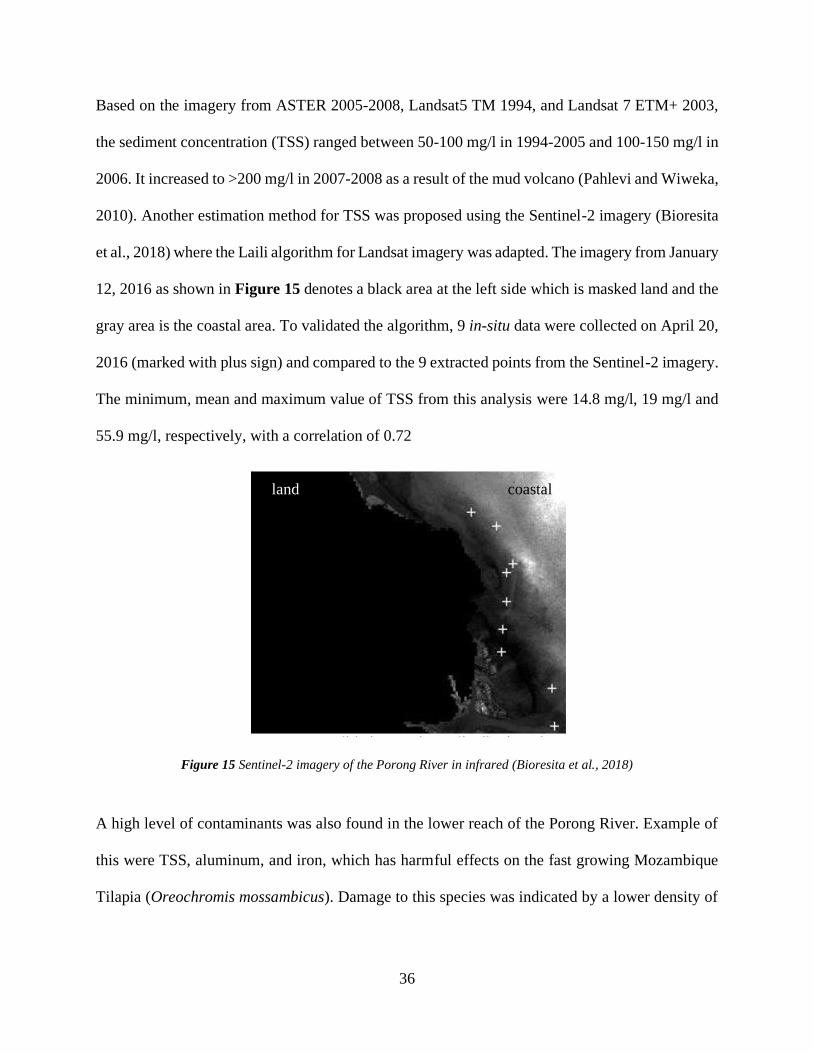
Sidoardjo, East Java as shown in Figure 16. More specifically, there are two craters of the
Sidoardjo Mud Volcano at 7o31’36.99”S and 112o42’41.90”E as shown in Figure 17. The volume
of the mud reservoir was about 40 million m3 with an area of 565 ha, a perimeter of 11 km and a
height of embankment of 15 m.
Figure 16 The location of Sidoardjo Mud Volcano
39
Figure 17 The recent photos of Sidoardjo Mud Volcano: a) bird view of the mud reservoir with the main crater in
the circle; b) the main crater of the Sidoardjo Mud Volcano
Figure 18 shows the evolution of the Sidoardjo Mud Volcano. The yellow arrow indicates the
main crater of the Sidoardjo Mud Volcano and the blue arrow indicates the flow direction of the
Porong River. In June 2006, the affected area was about 135 ha but the damage was still spreading.
From July 2010 to August 2018 as the figure shows, the mud volcano stabilized. Communities
were relocated and the mud reservoir had been constructed.
a)
b)
Craters

Figure 18 The evolution of Sidoardjo Mud Volcano taken with Google Earth (from left to right are pictures in 06/30/2006, 07/08/2010 and 08/07/2018,
respectively)
a) 06/30/2006 b) 07/18/2010 c) 08/07/2018
40
41
Figure 19 presents an embankment or mud reservoir map as managed by the Sidoardjo Mud
Control Agency in 2016. This was the public agency tasked with overseeing management and
mitigation of the mud volcano. The mud reservoirs were divided into several ponds based on the
location of former villages before the eruption. They are clockwise: Kedungbendo pond,
Glagaharum pond, Renokenongo pond, and Siring/Jatirejo pond. The agency also named the
embankments based on the order in which they were constructed. They start from P1 to P100. The
first 20 embankment points were located near the main crater and submerged due to the constant
eruption and subsidence. The most important points on the embankment are P25 (Jatirejo pond)
and P43 (Renokenongo pond). These are the location where pipes were installed to divert the mud.
There were 2 dredges at P25 (Jatirejo pond) and 4 dredges at P43 (Renokenongo pond). The name
of the outlet for P25 is Pejarakan Outlet (PO), located 16 km from the estuary while the outlet for
P43 (Renokenongo pond) is Ginonjo Outlet (GO), located 1 km downstream of the Pejarakan
Outlet. The recorded sediment concentration of the Pejarakan Outlet at the survey time was 40,000
mg/l or 𝐶𝑣 = 0.015, and the concentration of Ginonjo Outlets is 57,000 mg/l or 𝐶𝑣 = 0.022.

42
Figure 19 The 2016 Embankment maps of the mud reservoir
GO PO
P25 P43

43
3.2 Porong River
The Porong River is a tributary of Brantas River. The Porong River starts from Lengkong Baru
Weir in Mojokerto, East Java and is 50 km in length. The average bed slope is 28 cm/km. The
Porong River also receives water from Sadar Creek and Kambing Creek. For this research, the
study reach starts from upstream of the Ginonjo Outlet to its estuary at Madura Strait as indicated
by the blue bold line in Figure 20. The length of the study reach is 15.8 km. The Ginonjo and
Pejarakan Outlet’s pipe, are located on the left bank of the Porong River. Two important structures
near the study reach area are: a Porong station, which is 1.2 km upstream of Pejarakan Outlet,
records the stage of the Porong River and a scour protection structure devised to protect an
upstream bridge.
The quality of water is set out in Regulation 82 in 2001 (Indonesian Government, 2001). The
maximum total suspended sediment (TSS) for the Porong River as a class II river is 50 mg/l.
Figure 20 Plan view of the study reach in Porong River
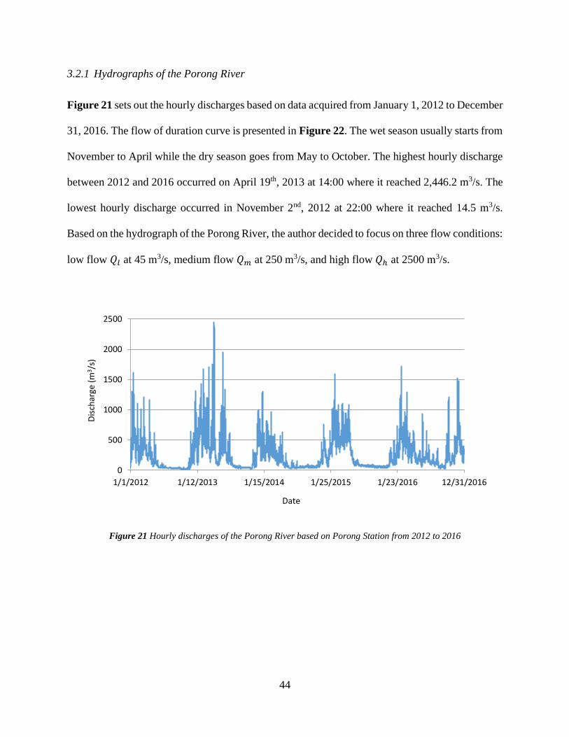
44
3.2.1 Hydrographs of the Porong River
Figure 21 sets out the hourly discharges based on data acquired from January 1, 2012 to December
31, 2016. The flow of duration curve is presented in Figure 22. The wet season usually starts from
November to April while the dry season goes from May to October. The highest hourly discharge
between 2012 and 2016 occurred on April 19th, 2013 at 14:00 where it reached 2,446.2 m3/s. The
lowest hourly discharge occurred in November 2nd, 2012 at 22:00 where it reached 14.5 m3/s.
Based on the hydrograph of the Porong River, the author decided to focus on three flow conditions:
low flow 𝑄𝑙 at 45 m3/s, medium flow 𝑄𝑚 at 250 m3/s, and high flow 𝑄ℎ at 2500 m3/s.
Figure 21 Hourly discharges of the Porong River based on Porong Station from 2012 to 2016
0
500
1000
1500
2000
2500
1/1/2012 1/12/2013 1/15/2014 1/25/2015 1/23/2016 12/31/2016
Dis
char
ge (
m3/s
)
Date

45
Figure 22 Flow duration curve of the Porong River
3.2.2 Hydraulic properties of the Porong River
The typical cross-section of the Porong River is shown in Figure 23. The location of the cross-
section, KP 168, is 30 m downstream of the Ginonjo Outlet. The bankfull width is about 160 m.
The hydraulic parameters for three flow conditions are presented in Table 5 which includes the
discharge (Q), average depth (h), top width (W), flow area (A), energy slope (Sf), average flow
velocity (V), and shear velocity (𝑢∗). The low flow 𝑄𝑙, which takes place in dry season between
June to November, has a flow depth, width, and velocity of 6.3 m, 106 m, and 0.1 m/s, respectively.
With limited flow velocity, the diverted mud was expected to have more time for mixing and
settling. This is the main concern for this research. The medium flow (𝑄𝑚 = 250 m3/s), which
usually takes place during wet season, would have a flow depth, width, and average velocity of
6.33 m, 106 m, and 0.57 m/s, respectively. In this condition, the diverted mud would have less
1
10
100
1000
10000
0.00001 0.0001 0.001 0.01 0.1 1
Dis
char
ge (
m3/s
)
Exceedence Probability
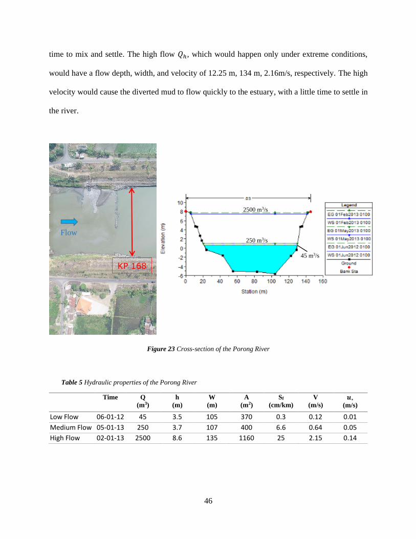
46
time to mix and settle. The high flow 𝑄ℎ, which would happen only under extreme conditions,
would have a flow depth, width, and velocity of 12.25 m, 134 m, 2.16m/s, respectively. The high
velocity would cause the diverted mud to flow quickly to the estuary, with a little time to settle in
the river.
Figure 23 Cross-section of the Porong River
Table 5 Hydraulic properties of the Porong River
Time Q
(m3)
h
(m)
W
(m)
A
(m2)
Sf
(cm/km)
V
(m/s)
𝒖∗ (m/s)
Low Flow 06-01-12 45 3.5 105 370 0.3 0.12 0.01
Medium Flow 05-01-13 250 3.7 107 400 6.6 0.64 0.05
High Flow 02-01-13 2500 8.6 135 1160 25 2.15 0.14
KP 168
2500 m3/s
250 m3/s
45 m3/s
Flow

47
3.2.3 Characteristics of bed materials
We investigated the particle size distribution of the bed material at three different locations, as
described in Figure 24: Bed1, which is located at 500 m upstream of the Pejarakan Outlet (original
condition), Bed2, which is located at 10 km downstream of the Ginonjo Outlet, and Bed3, which
is located at 13 km downstream of the Ginonjo Outlet. The results are presented on Figure 25
(Laboratorium Mekanika Tanah dan Batuan, 2018). Bed1 was found to consist of 0.2% gravel,
43.2% sand, 47.7% silt, and 8.9% clay. Bed2 was found to consist of 15.6% sand, 69.9% silt, and
14.5% clay. Bed3 was found to consist of 0.2% gravel, 47.8% sand, 48.7% silt, and 3.3% clay.
Figure 24 Location of the sampling of bed material in the Porong River, Sidoardjo, East Java
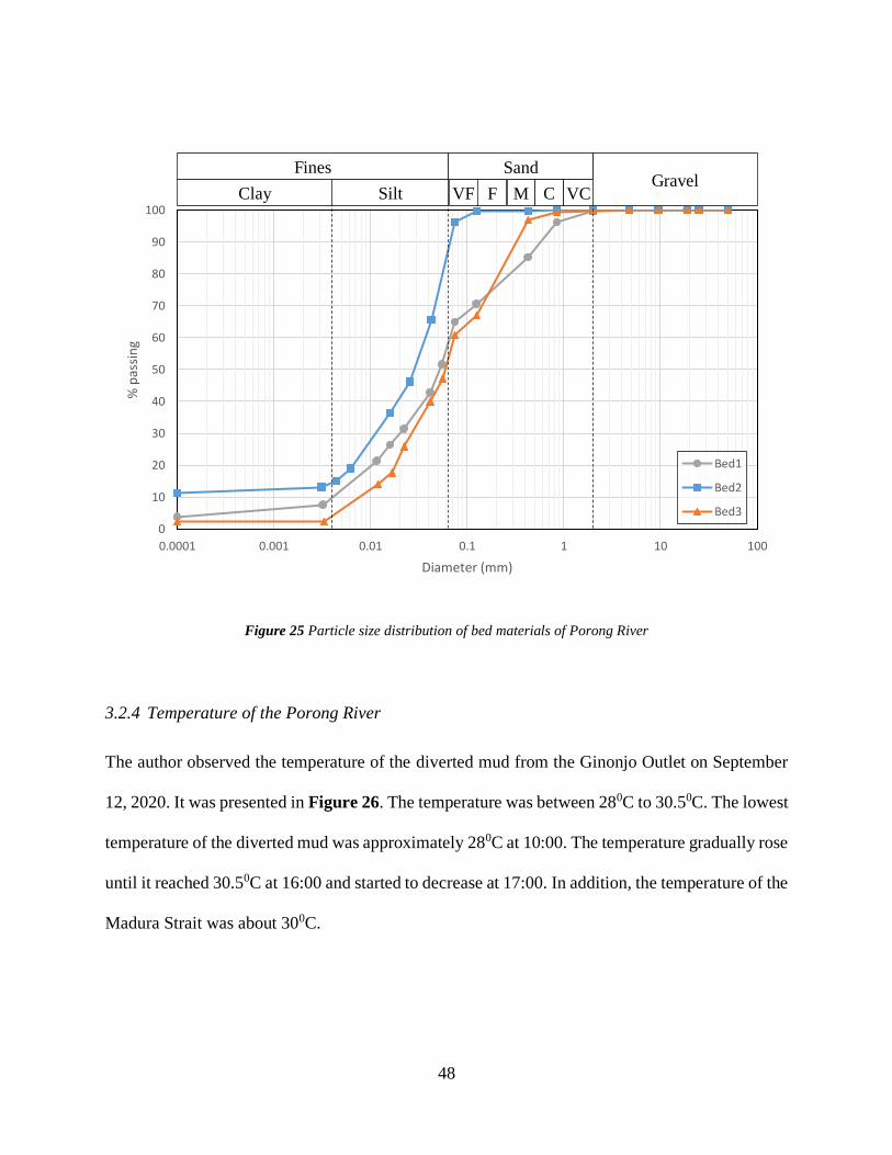
48
Figure 25 Particle size distribution of bed materials of Porong River
3.2.4 Temperature of the Porong River
The author observed the temperature of the diverted mud from the Ginonjo Outlet on September
12, 2020. It was presented in Figure 26. The temperature was between 280C to 30.50C. The lowest
temperature of the diverted mud was approximately 280C at 10:00. The temperature gradually rose
until it reached 30.50C at 16:00 and started to decrease at 17:00. In addition, the temperature of the
Madura Strait was about 300C.
0
10
20
30
40
50
60
70
80
90
100
0.0001 0.001 0.01 0.1 1 10 100
% p
assi
ng
Diameter (mm)
Bed1
Bed2
Bed3
C
Fines
SiltClay
SandGravel
VCMFVF

49
Figure 26 Temperature of the diverted mud from Ginonjo Outlet on September 12, 2020
The temperature of flow of the Porong River on September 12, 2020 is presented in Figure 27.
Based on Figure 27, the range of temperature of the flow ranged between 29.10C to 29.80C. The
lowest temperature was observed at around 9:00 to 10:00 while the highest temperature was
recorded at 14:00 to 17:00. The average temperature of this day was 29.50C.
The temperature of flow of the Porong River also had been observed on October 14-15, 2020 as
shown in Figure 28. In these two days, the temperature was between 310C to 340C with an average
temperature of 32.50C. The highest temperature was recorded at 15:00 on October 14, 2020. Even
though there were fluctuations at around 23:00, the temperature gradually decreased to 330C at
13:00 and more rapidly decreased to 310C at 7:00 on October 15, 2020. Then, the temperature
slowly increased at 11:00. Based on the data from September 12 and October 14-15, the lowest
temperature occurs around 10:00 in the morning and the highest temperature usually occurs at
15:00.
27.5
28
28.5
29
29.5
30
30.5
31
8:00 10:00 12:00 14:00 16:00 18:00
Tem
per
atu
re (
0C
)
Time
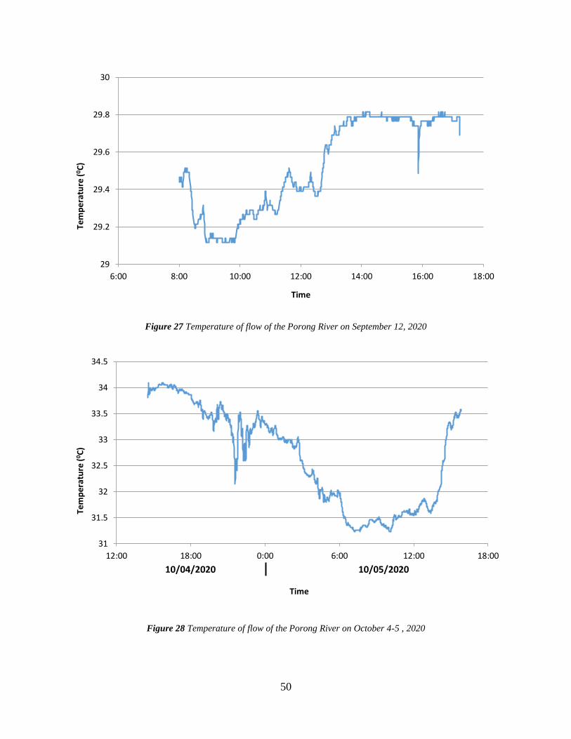
50
Figure 27 Temperature of flow of the Porong River on September 12, 2020
Figure 28 Temperature of flow of the Porong River on October 4-5 , 2020
29
29.2
29.4
29.6
29.8
30
6:00 8:00 10:00 12:00 14:00 16:00 18:00
Tem
per
atu
re (
0C
)
Time
31
31.5
32
32.5
33
33.5
34
34.5
12:00 18:00 0:00 6:00 12:00 18:00
Tem
per
atu
re (
0C
)
Time
10/04/2020 10/05/2020

51
CHAPTER 4 THE PROPERTIES OF THE DIVERTED MUD
4.1 Particle Size Distribution of Mud Samples
To determine the physical characteristics of the mud, a particle size distribution analysis of the
mud was completed. The author sampled the extruded mud, taken near the main crater (P25), and
mud that had been diverted from the Pejarakan and Ginonjo Outlets. The particle size distribution
analysis was completed at Transportation and Geotechnical Laboratory of Civil Engineering of
Sepuluh November Institute of Technology in Manyar, Surabaya. Figure 29 shows the particle
size distributions for these samples (Laboratorium Transportasi dan Geoteknik, 2018), which
consists mainly of silts and clays. The extruded mud has 17.1% sand, 44% silt, and 38.9% clay;
mud diverted from the Pejarakan Outlet has 5.2% sand, 41.2% silt, and 53.6% clay; and mud
diverted from the Ginonjo Outlet has 0.8% gravel, 13.3% sand, 34.1% silt, and 51.8% clay. The
median grain size or d50 and the gradation coefficient for these samples are shown in Table 6.
Table 6 The grain size and gradient coefficient of mud samples
Sample d10 (mm) d50 (mm) d80 (mm) Gr (-)
Extruded Mud 0.0013 0.0080 0.0526 6.48
Diverted Mud – Pejarakan 0.0010 0.0034 0.0216 5.63
Diverted Mud - Ginonjo 0.0011 0.0047 0.0556 8.85

52
Figure 29 Particle size distribution of mud samples (VC: very coarse, C: coarse, M: medium, F: fine, and VF: very
fine)
0
10
20
30
40
50
60
70
80
90
100
0.0001 0.001 0.01 0.1 1 10 100
% p
assi
ng
Diameter (mm)
Extruded Mud
Diverted Mud - Pejarakan
Diverted Mud - Ginonjo
C
Fines
SiltClay
SandGravel
VCMFVF
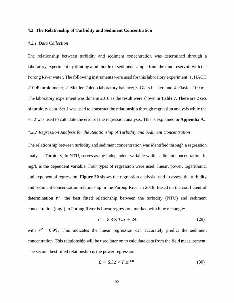
53
4.2 The Relationship of Turbidity and Sediment Concentration
4.2.1 Data Collection
The relationship between turbidity and sediment concentration was determined through a
laboratory experiment by diluting a full bottle of sediment sample from the mud reservoir with the
Porong River water. The following instruments were used for this laboratory experiment: 1. HACH
2100P turbidimeter; 2. Mettler Toledo laboratory balance; 3. Glass beaker; and 4. Flask – 100 ml.
The laboratory experiment was done in 2018 as the result were shown in Table 7. There are 2 sets
of turbidity data. Set 1 was used to construct the relationship through regression analysis while the
set 2 was used to calculate the error of the regression analysis. This is explained in Appendix A.
4.2.2 Regression Analysis for the Relationship of Turbidity and Sediment Concentration
The relationship between turbidity and sediment concentration was identified through a regression
analysis. Turbidity, in NTU, serves as the independent variable while sediment concentration, in
mg/l, is the dependent variable. Four types of regression were used: linear, power, logarithmic,
and exponential regression. Figure 30 shows the regression analysis used to assess the turbidity
and sediment concentration relationship in the Porong River in 2018. Based on the coefficient of
determination 𝑟2, the best fitted relationship between the turbidity (NTU) and sediment
concentration (mg/l) in Porong River is linear regression, marked with blue rectangle:
𝐶 = 5.3 × 𝑇𝑢𝑟 + 24 (29)
with 𝑟2 = 0.99. This indicates the linear regression can accurately predict the sediment
concentration. This relationship will be used later on to calculate data from the field measurement.
The second best fitted relationship is the power regression:
𝐶 = 5.32 × 𝑇𝑢𝑟1.01 (30)

54
with 𝑟2 = 0.99. While it has a good accuracy for the lower values of concentration, it tends to
overpredict the concentration at higher values.
Table 7 Turbidity (NTU) of the sediment mixture of the corresponding sediment concentration from the laboratory
experiment in 2018
No. C (mg/L) Turbidity (NTU)
1 2
1 5000.0 949.0 962.0
2 2500.0 469.0 504.0
3 1666.7 255.0 295.0
4 1250.0 245.0 243.0
5 1000.0 189.0 180.0
6 833.3 172.0 143.0
7 714.3 119.0 94.7
8 625.0 110.0 108.0
9 555.6 94.5 107.0
10 500.0 69.4 75.1
11 476.2 84.4 90.3
12 454.5 88.3 84.6
13 416.7 66.6 68.7
14 384.6 64.0 70.4
15 357.1 56.8 59.3
16 333.3 61.9 59.7
17 312.5 54.4 57.9
18 277.8 51.4 47.3
19 250.0 42.4 39.1
20 166.7 24.9 28.1
21 125.0 22.8 22.6
22 100.0 17.2 18.0
23 83.3 16.0 17.1
24 71.4 11.9 12.8
25 62.5 10.9 11.4
26 55.6 10.7 10.4
27 50.0 8.2 8.4
28 45.5 7.8 7.8
29 41.7 7.0 7.5
30 35.7 7.1 6.6
31 31.3 6.3 6.1
32 27.8 5.6 6.1
33 25.0 6.7 6.1

55
Figure 30 Regression analysis for turbidity and sediment concentration in Porong River in 2018
Figure 31 compares preliminary results from previous studies of the relationship of turbidity and
sediment concentration. The preliminary results (red circle) is plotted in the middle of the previous
studies.
y = 5.2974x + 23.962R² = 0.9955
0
1000
2000
3000
4000
5000
6000
0 200 400 600 800 1000
Co
nce
ntr
atio
n (
mg/
L)
Turbidity (NTU)
Linear Regression
y = 526.92ln(x) - 1386R² = 0.582
-1000
0
1000
2000
3000
4000
5000
6000
0 200 400 600 800 1000
Co
nce
ntr
atio
n (
mg/
L)
Turbidity (NTU)
Logarithmic Regression
y = 5.3187x1.0134
R² = 0.9951
0
1000
2000
3000
4000
5000
6000
0 200 400 600 800 1000
Co
nce
ntr
atio
n (
mg/
L)
Turbidity (NTU)
Power Regression
y = 127.06e0.0057x
R² = 0.739
0
5000
10000
15000
20000
25000
30000
35000
0 200 400 600 800 1000
Co
nce
ntr
atio
n (
mg/
L)
Turbidity (NTU)
Exponential Regression

56
Figure 31 Comparison of the relationship of turbidity and sediment concentration between the preliminary result
and previous studies
4.3 Flocculation
Flocculation tests were conducted in December 2019 to determine the flocculation processes in
the mixture. Two samples were prepared for flocculation tests. The deflocculant agent (specified
in the previous chapter) was added to one of the samples while leaving the other sample untouched.
Both samples were shaken to resuspend the sediment to compare the settling time and settling
distance time. If flocculation occurs, the sample with deflocculant should settle slower than the
sample without deflocculant. Otherwise, both will settle around similar time frame. The hyphotesis
was that flocculation occurs because fine sediments dominate the mud mixtures.

57
Water samples from each diversion outlet were gathered and poured into 500ml bottles and
catalogued to identify the diversion outlet, as shown in Figure 32. Two bottles containing water
collected from Pejarakan Outlet were named P1 and P2 and two bottles containing water collected
from Ginonjo Outlet were named G1 and G2. P1 and G1 were without the deflocculant while P2
and G2 were mixed with 5 ml of the deflocculant. The sediment was left to settle and the settling
distance and settling time were recorded.
Figure 32 Samples from Pejarakan and Ginonjo Outlet. Sample from left: P1, P2, G1 and G2; deflocculant were
added to P2 and G2.
Figure 33 shows the comparative result of the flocculation test during the first 4 hours of the
experiment. The settling velocity is settling distance divided by settling time. Comparing the result
of those samples, the settling velocity of sample mixed with deflocculant P2 was slower than the
settling velocity of the natural sample P1. The settling velocity of P2 was 0.015 mm/s while P1
1
1 2 2

58
was 0.032 mm/s. Both were recorded 10 minutes after the test was started. For G1 and G2, the
fastest settling velocity were at 0.028 mm/s and 0.013 mm/s, respectively. By comparing the
settling velocity between the samples from Pejarakan and Ginonjo, it is possible to summarize that
samples from Pejarakan had a slightly faster settling velocity. Thus, the mud from Pejarakan Outlet
settled faster than the mud from Ginonjo. The settling velocity value of the two outlets was
miniscule compared to the general settling velocity, which is 0.15 – 0.6 mm/s. Nevertheless, the
test concluded that the mud has a very slight tendency to flocculate.
Figure 33 Results of flocculation test
Furthermore, the settling velocity gradually decreased after 60 minutes because the coarser
particles have settled to the bottom of the bottle. The research also analyzed ratios of settling
velocity between the samples with and without deflocculant as presented in Figure 34. The settling
velocity of samples without deflocculant were 2.1 times higher than the settling velocity of samples
with deflocculant. These ratio kept decreasing over 60 minutes until it reached 1.4 and 1.3 for
0.000
0.005
0.010
0.015
0.020
0.025
0.030
0.035
0 50 100 150 200 250
Sett
ling
Vel
oci
ty (
mm
/s)
Time (min)
Flocculation Test
P1 - Original
P2 - Defloc
G1 - Original
G2 - Defloc

59
sample from Pejarakan and Ginonjo, respectively. After 60 minutes, the ratio stabilized at an
average of 1.2 for Pejarakan’s sample and 1.25 for Ginonjo’s sample. This indicated that a portion
of sediment forms a bigger floc, as a flocculation process, and settled after 60 minutes. The non-
flocculated sediments started to become visible after 60 minutes.
Figure 34 Ratio of settling velocity of deflocculated samples and original samples
1.0
1.2
1.4
1.6
1.8
2.0
2.2
0 50 100 150 200 250
Rat
io
Time (min)
Pejarakan
Ginonjo

60
CHAPTER 5 FIELD MEASUREMENTS
The objective of the field measurements was to validate the computational model. The field
measurements were needed because a comprehensive data set was not available. Two field
measurements were conducted in the study reach: Field measurement program #1 in July 10-14,
2018 and Field measurement program #2 in September 10-12, 2019.
5.1 Field Measurement Program #1 (July 10-14, 2018)
The field program measured turbidity along the whole study reach. The turbidity data can be easily
measured and are used as a surrogate of sediment concentration. At the time of the measurements
#1, the discharge of the Porong River is 45.2 m3/s with flow velocity of 0.16 m/s and shear velocity
of 0.01 m/s. The upstream sediment concentration was 56.7 mg/l. The sediment concentration of
the diverted mud at Ginonjo Outlet is 57,000 mg/l and the discharge was 0.33 m3/s. The following
is the field survey program with point measurements.
The river reach of 15.8 km was surveyed at 106 cross-sections with a distance between cross-
sections of 150 m. The first cross-section of the measurement was located at 30 m upstream of
Ginonjo Outlet and was intended to capture the undisturbed sediment concentration in the Porong
River. The second cross-section was at 80 m downstream of the Ginonjo Outlet. The following
cross-section up to the 106th cross-section were located 150 m downstream of the previous cross-
section. Each cross-section had 4 point of measurements with a lateral distance between point
measurements of 25 m as illustrated in Figure 35. For example, cross-section 1 consists of points
1A, 1B, 1C, and 1D. Cross sections were offset by 5 m from the left and right bank to avoid
additional sediment concentration from the river bank.

61
Figure 35 Illustration of field measurement #1 in the study reach; not to scale (point A, B, C, and D illustrated the 4
points of measurement in one cross-section)
The field measurements were carried out at 1 m below the water surface. An instantaneous sampler
was used with a product name of water sampler horizontal “bit” type WSH-BIT 22 that had a
capacity of 2.2L as shown in Figure 36. Then, the turbidity of the sample was measured by using
a turbidimeter and the coordinate at the collection point were recorded. Figure 37 presents the
pictures when the measurements were completed on the field. The turbidity data from field
measurement #1 were presented in Appendix B.
Figure 36 Water sampler horizontal for field measurements
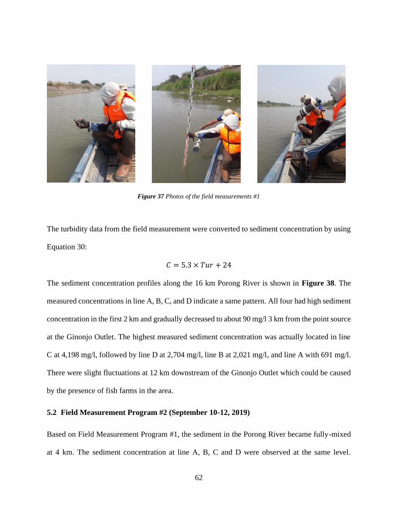
62
Figure 37 Photos of the field measurements #1
The turbidity data from the field measurement were converted to sediment concentration by using
Equation 30:
𝐶 = 5.3 × 𝑇𝑢𝑟 + 24
The sediment concentration profiles along the 16 km Porong River is shown in Figure 38. The
measured concentrations in line A, B, C, and D indicate a same pattern. All four had high sediment
concentration in the first 2 km and gradually decreased to about 90 mg/l 3 km from the point source
at the Ginonjo Outlet. The highest measured sediment concentration was actually located in line
C at 4,198 mg/l, followed by line D at 2,704 mg/l, line B at 2,021 mg/l, and line A with 691 mg/l.
There were slight fluctuations at 12 km downstream of the Ginonjo Outlet which could be caused
by the presence of fish farms in the area.
5.2 Field Measurement Program #2 (September 10-12, 2019)
Based on Field Measurement Program #1, the sediment in the Porong River became fully-mixed
at 4 km. The sediment concentration at line A, B, C and D were observed at the same level.

63
However, from 0 to 4 km, there were different sediment concentrations laterally and perhaps
vertically. Therefore, the Field Measurement Program #2 aimed to capture the vertical variability
of sediment concentration, or the vertical sediment concentration profile for the first 4 km of the
study reach. Field Measurement Program #2 was completed in September 20-12, 2019. The
discharge of the Porong River was 47.7 m/s, flow velocity was 0.16 m/s and the shear velocity
was 0.01 m/s.
Figure 38 The measured sediment concentration in the study reach
The points of measurements in field measurement #2 were presented in Figure 39. Similar to Field
Measurement #1, each cross-section had 4 point of measurements with the lateral distance between
each point was 25 m and had 5 m offset from the left and right bank. The first cross-section was
at 130 m downstream of the Ginonjo Outlet. For the first 4 km, the following cross-section was
located 100 m downstream of the previous cross-section. After 4 km, the distance between cross-
section was 200 m. The first cross-section could not be closer to the Ginonjo Outlet because there
10
100
1000
10000
0 2 4 6 8 10 12 14 16
Co
nce
ntr
atio
n(m
g/L)
Distance (km)
Measured Concentration
A B C D

64
were a ground sill or river bed protection consists of many tetrapods at 30 m downstream of the
outlet. To capture the vertical sediment concentration, the sample were taken every 1 m depth until
the bed of the Porong River. This action was done at each point measurement. Field Measurement
#2 also utilized the instantaneous sampler as shown in Figure 36. Documentations of the
measurement were shown in Figure 40. In total 301 bottles os sample were collected.
Figure 39 Illustration of field measurement #2 in the study reach; not to scale (point A, B, C, and D illustrated the 4
points of measurement in one cross-section)
Figure 40 Photos of field measurements and bottles of samples
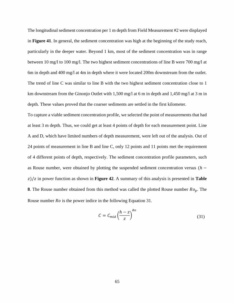
65
The longitudinal sediment concentration per 1 m depth from Field Measurement #2 were displayed
in Figure 41. In general, the sediment concentration was high at the beginning of the study reach,
particularly in the deeper water. Beyond 1 km, most of the sediment concentration was in range
between 10 mg/l to 100 mg/l. The two highest sediment concentrations of line B were 700 mg/l at
6m in depth and 400 mg/l at 4m in depth where it were located 200m downstream from the outlet.
The trend of line C was similar to line B with the two highest sediment concentration close to 1
km downstream from the Ginonjo Outlet with 1,500 mg/l at 6 m in depth and 1,450 mg/l at 3 m in
depth. These values proved that the coarser sediments are settled in the first kilometer.
To capture a viable sediment concentration profile, we selected the point of measurements that had
at least 3 m depth. Thus, we could get at least 4 points of depth for each measurement point. Line
A and D, which have limited numbers of depth measurement, were left out of the analysis. Out of
24 points of measurement in line B and line C, only 12 points and 11 points met the requirement
of 4 different points of depth, respectively. The sediment concentration profile parameters, such
as Rouse number, were obtained by plotting the suspended sediment concentration versus (ℎ −
𝑧)/𝑧 in power function as shown in Figure 42. A summary of this analysis is presented in Table
8. The Rouse number obtained from this method was called the plotted Rouse number 𝑅𝑜𝑝. The
Rouse number 𝑅𝑜 is the power indice in the following Equation 31.
𝐶 = 𝐶𝑚𝑖𝑑 (
ℎ − 𝑧
𝑧)𝑅𝑜
(31)
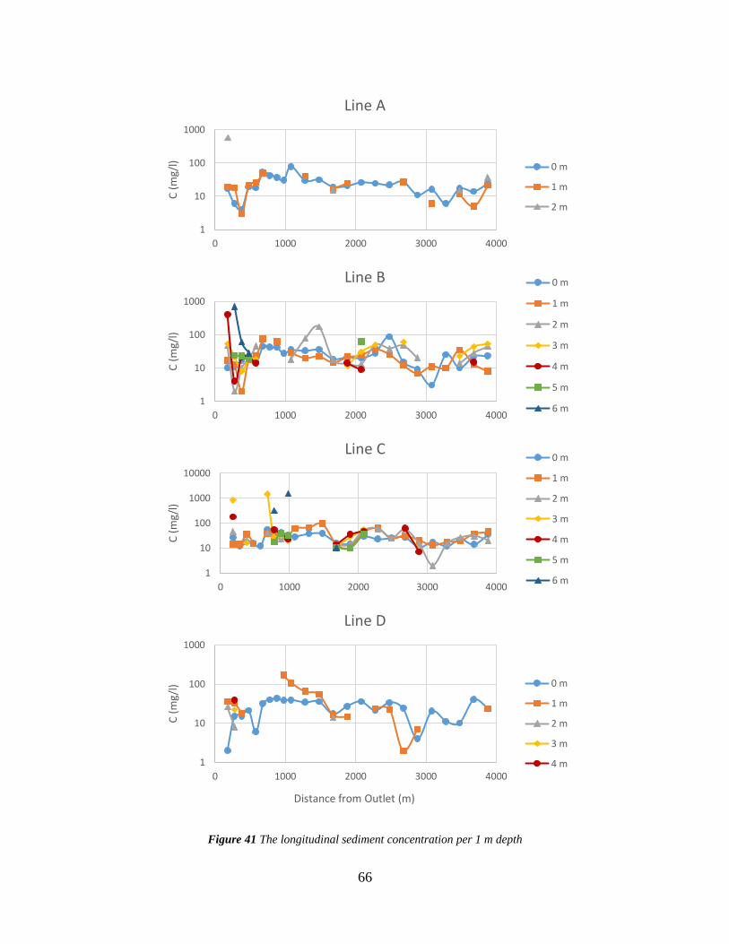
66
Figure 41 The longitudinal sediment concentration per 1 m depth
1
10
100
1000
0 1000 2000 3000 4000
C (
mg/
l)
Line A
0 m
1 m
2 m
1
10
100
1000
0 1000 2000 3000 4000
C (
mg/
l)
Line B 0 m
1 m
2 m
3 m
4 m
5 m
6 m
1
10
100
1000
10000
0 1000 2000 3000 4000
C (
mg/
l)
Line C0 m
1 m
2 m
3 m
4 m
5 m
6 m
1
10
100
1000
0 1000 2000 3000 4000
C (
mg/
l)
Distance from Outlet (m)
Line D
0 m
1 m
2 m
3 m
4 m

67
Figure 42 Plot of suspended sediment concentration versus (ℎ − 𝑧)/𝑧
1
10
100
1000
0.001 0.01 0.1 1 10 100
C (
mg/
l
(h-z)/z
Line B 1234514151618222324Power (1)Power (2)Power (3)Power (4)Power (5)Power (14)Power (15)Power (16)Power (18)Power (22)Power (23)Power (24)
1
10
100
1000
10000
0.001 0.01 0.1 1 10 100
C (
mg/
l
(h-z)/z
Line C1367891314151819Power (1)Power (3)Power (6)Power (7)Power (8)Power (9)Power (13)Power (14)Power (15)Power (18)Power (19)

68
Table 8 Summary of the analysis of sediment concentration parameter (ℎ is the flow depth;𝑅𝑜𝑝 is the plotted Rouse
number; 𝐶𝑚𝑖𝑑 is the mid-depth sediment concentration; 𝐶𝑎 is the reference sediment concentration which in this
case is the near-bed concentration)
XS Line B Line C
h (m) Rop Cmid (mg/l) Ca (mg/l) h (m) Rop Cmid (mg/l) Ca (mg/l)
1 4.1 0.36 53.23 401 4.5 0.31 101.09 175
2 6.1 0.31 19.13 702 - - - -
3 6.6 0.13 15 61 3.6 0.01 21.1 16
4 6.1 0.03 20.56 28 - - - -
5 4.3 0.02 21.09 14 - - - -
6 - - - - 3.1 0.29 124.29 1448
7 - - - - 6.1 0.16 43.85 310
8 - - - - 5.4 0 32.34 39
9 - - - - 6.1 0.27 50.37 1504
13 - - - - 6.1 0 12.16 10
14 4.6 0 14.85 14 5.5 0.03 16.85 10
15 5.1 0.07 22.13 62 5.1 0.04 43.73 38
16 4.5 0.09 46.57 51 - - - -
18 3.8 0.18 34.67 61 4.9 0.11 19.54 61
19 - - - - 4.2 0 10.91 7
22 4.0 0.11 21.34 23 - - - -
23 4.1 0 21.98 15 - - - -
24 3.9 0.09 29.42 53 - - - -
Based on Figure 42 and Table 8, the plotted Rouse number 𝑅𝑜𝑝 ranged from 0 to 0.36, which is
smaller than 1.25 as the limit of the mixed load. Therefore, the mode of sediment transport in the
study reach is suspended load. It can be assumed that the concentration profile are a uniform (𝑅𝑜 =
0).
A deeper investigation for 6 cross-section with the highest plotted Rouse number was completed.
These were cross-section (XS) B-1, B-2, B-18, C-1, C-6, and C-9 as presented in Table 9 and
Figure 43. There were 3 types of sediment concentration profiles in Figure 43: measured
concentration profiles from sampling or measurements, fitted concentration profiles obtained by
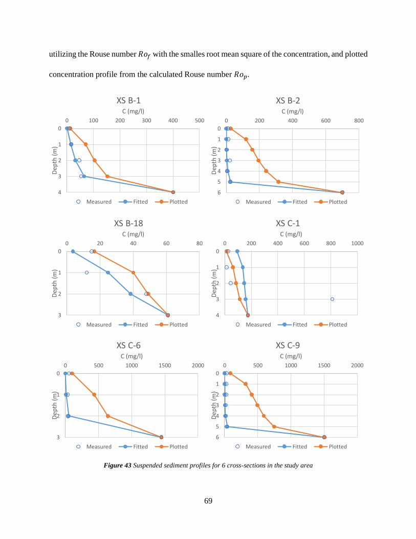
69
utilizing the Rouse number 𝑅𝑜𝑓 with the smalles root mean square of the concentration, and plotted
concentration profile from the calculated Rouse number 𝑅𝑜𝑝.
0
1
2
3
4
0 100 200 300 400 500
Dep
th (
m)
C (mg/l)
XS B-1
Measured Fitted Plotted
0
1
2
3
4
5
6
0 200 400 600 800
Dep
th (
m)
C (mg/l)
XS B-2
Measured Fitted Plotted
0
1
2
3
0 20 40 60 80
Dep
th (
m)
C (mg/l)
XS B-18
Measured Fitted Plotted
0
1
2
3
4
0 200 400 600 800 1000
Dep
th (
m)
C (mg/l)
XS C-1
Measured Fitted Plotted
0
1
2
3
0 500 1000 1500 2000
De
pth
(m
)
C (mg/l)
XS C-6
Measured Fitted Plotted
0
1
2
3
4
5
6
0 500 1000 1500 2000
Dep
th (
m)
C (mg/l)
XS C-9
Measured Fitted Plotted
Figure 43 Suspended sediment profiles for 6 cross-sections in the study area

70
Table 9 Suspended sediment concentration parameters for 6 cross-sections in the study area
XS h (m)
Cmid (mg/l)
Ca (mg/l)
Rof ds (mm)
RMSf Roc ds (mm)
RMSc
B-1 4.1 53 401 0.68 49 9 0.36 36 56.37
B-2 6.1 19 702 1.27 68 10 0.31 33 171.94
B-18 3.8 35 61 0.39 50 10 0.18 25 14.10
C-1 4.5 101 175 0.07 16 303 0.31 33 313.96
C-6 3.1 124 1448 1.22 67 31 0.29 32 361.99
C-9 6.1 50 1504 1.40 72 19 0.27 31 431.72
Figure 43 shows that the plotted sediment concentration profiles did not fit the measured
concentration profiles. The root mean square between those two profiles ranged from 14.1 to 431.
Meanwhile, the root mean square between the fitted concentration profiles and the measured
concentration profiles ranged from 9 to 303. The results of median grain size for fitted
concentration profiles ranged from very fine sand to medium silt, while for the plotted
concentration profiles ranged from coarse silt to medium silt. Therefore, the results from the fitted
concentration profiles is more appropriate to use for modeling. The median grain size of the
diverted mud was very fine silt, as mentioned in Table 6. It then changed into medium silt because
of flocculation.

71
CHAPTER 6 SEDIMENT PROPAGATION MODEL FOR THE PORONG RIVER
6.1 HEC-RAS
The objective of the HEC-RAS model used in this research is to understand the hydraulic
properties in the Porong River. To achieve this objective, the HEC-RAS model with the quasi
unsteady flow and the sediment transport was utilized. The results obtained from the HEC-RAS,
such as the river width, flow depth, and average flow velocity, are therefore necessary for the
sediment propagation model. There are three main inputs for the HEC-RAS simulation. They are:
geometric data, quasi unsteady flow data, and sediment data. The geometric data were obtained
from the study reach characteristics with a plan view of the Porong River as in Figure 44.
Figure 44 Plan view of the study reach in HEC-RAS (GO is Ginonjo Outlet)
The cross-section in the study reach are featured in Figure 45. We analyzed 26 cross-sections
throughout the study reach. The Ginonjo Outlet is located just upstream of KP 168 (or cross-section
46) in HEC-RAS and there are 4 cross-sections upstream of the outlet. The bed slope of the study
GO
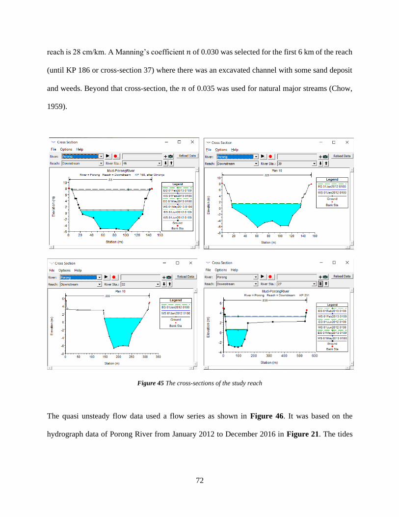
72
reach is 28 cm/km. A Manning’s coefficient 𝑛 of 0.030 was selected for the first 6 km of the reach
(until KP 186 or cross-section 37) where there was an excavated channel with some sand deposit
and weeds. Beyond that cross-section, the 𝑛 of 0.035 was used for natural major streams (Chow,
1959).
Figure 45 The cross-sections of the study reach
The quasi unsteady flow data used a flow series as shown in Figure 46. It was based on the
hydrograph data of Porong River from January 2012 to December 2016 in Figure 21. The tides

73
prediction data (Geospatial Information Agency, 2019) were used for the downstream boundary
condition as shown in Figure 47 with 0.0 m indicates the mean sea level.
Figure 46 Flow series of the study reach for 2012-2016
Figure 47 Tides in Madura Strait
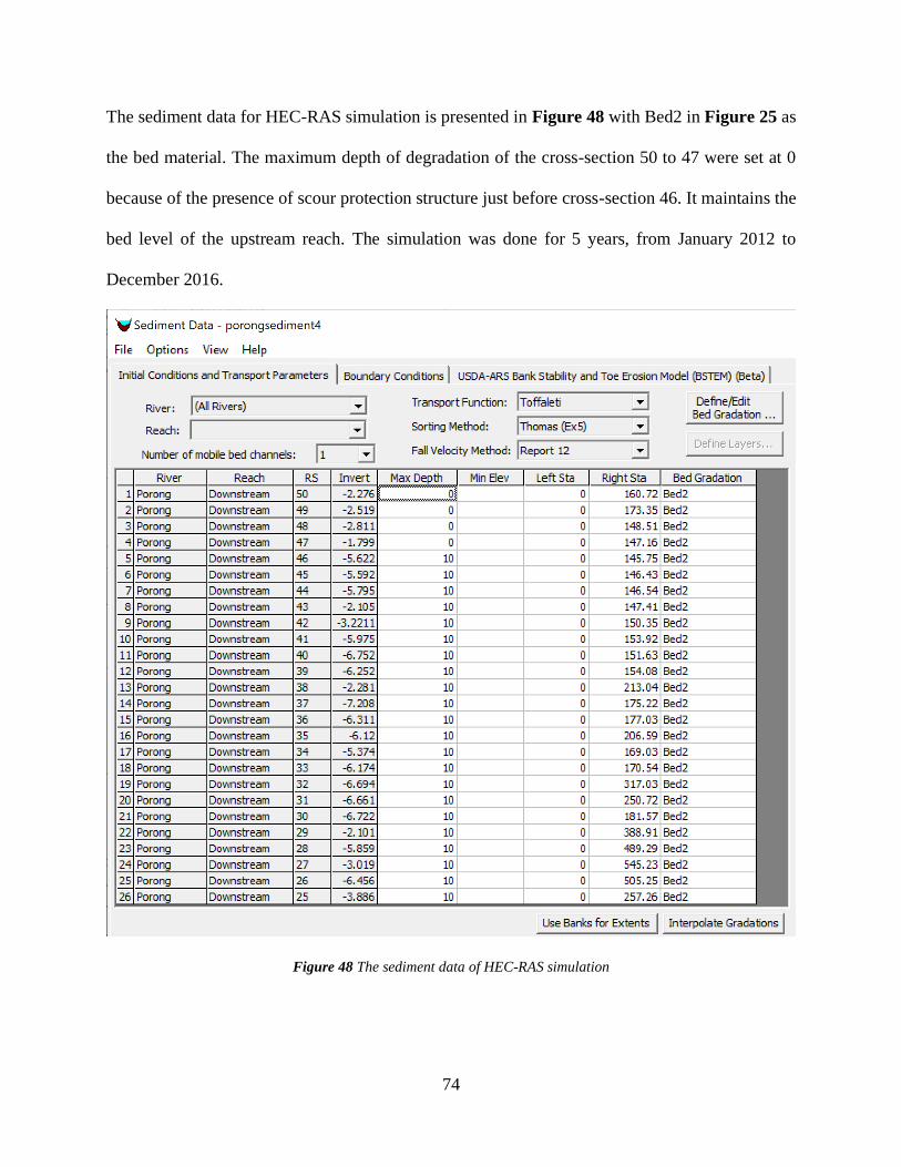
74
The sediment data for HEC-RAS simulation is presented in Figure 48 with Bed2 in Figure 25 as
the bed material. The maximum depth of degradation of the cross-section 50 to 47 were set at 0
because of the presence of scour protection structure just before cross-section 46. It maintains the
bed level of the upstream reach. The simulation was done for 5 years, from January 2012 to
December 2016.
Figure 48 The sediment data of HEC-RAS simulation

75
The results of the HEC-RAS are shown in Figure 49. It shows the bed elevation changes and water
surface elevation in longitudinal plane for 4 different dates: (a) January 1, 2012, as the initial
condition; (b) June 1, 2012, for the low flow condition; (c) Feb 1, 2013, for the high flow condition;
and (d) May 1, 2013, for the medium flow condition. Aggradation was spotted in the first km from
the Ginonjo Outlet (GO) while degradation was spotted at approximately 1.5 km and at the
downstream end of the study reach. At cross-section 46, there were about 4 m of aggradation over
5 years due to the sedimentation of coarse sediment. There were no significant change in the bed
elevation for cross-section 39 and 32. At cross-section 27, high degradation was spotted only at
the first day. Appendix C presents the sediment time series for 4 cross-sections.
Figure 49 The water surface elevation of the study reach from HEC-RAS simulation ( indicates flow direction
and GO is Ginonjo Outlet)
Downstream
end
𝑄𝑚𝑎𝑦 = 250 𝑚3/𝑠
𝑄𝑓𝑒𝑏 = 2500 𝑚3/𝑠
𝑄𝑗𝑢𝑛 = 45 𝑚3/𝑠
𝑄𝑗𝑎𝑛 = 500 𝑚3/𝑠
GO

76
6.2 Two-Dimensional Mixing Model
Results from HEC-RAS simulation such as the hydraulic properties of the Porong River are used
to solve the advection-diffusion equation. Table 10 summaries the first order approximation of the
coefficient, length and time scale of longitudinal dispersion, vertical and transversal mixing of the
Porong River.
Table 10 Summary of the coefficitent, length and time scale of longitudinal dispersion, vertical and transversal
mixing of the Porong River
𝑲𝒅
(𝒎𝟐/𝒔) 𝜺𝒗
(𝒎𝟐/𝒔) 𝜺𝒕
(𝒎𝟐/𝒔) 𝑿𝒅
(m)
𝑿𝒗
(m)
𝑿𝒕 (m)
𝒕𝒅
(s)
𝒕𝒗
(s)
𝒕𝒕 (s)
Low Flow 85 0.02 0.20 1,420 43 3,920 11,800 355 32,660
Medium Flow 95 0.03 0.23 300 240 19,260 460 370 30,100
High Flow 330 0.09 0.80 290 1,200 29,250 145 560 13,600
As described in the site description, the Ginonjo Outlet is located in the left bank with 57,000 mg/l
sediment concentration of the diverted mud. This corresponds to 0.02 concentration by volume 𝐶𝑣.
Theoretically, the sediment concentration should be high near the left bank because it is close to
the outlet and should be low at the right bank of the river. This phenomena should be found in the
first couple km of the reach, or before the diverted mud becomes fully-mixed. The fully-mixed
sediment concentration 𝐶𝑏 was calculated by using Equation 24. Assume a low flow condition of
the Porong River of 45 m3/s, initial sediment concentration was 56.7 mg/l, the discharge of the
diverted mud from Ginonjo outlet was 0.33 m3/s and the sediment concentration of the diverted
mud was 57,000 mg/l. Thus:
𝐶𝑏 =
𝐶𝑜𝑢𝑡𝑙𝑒𝑡 × 𝑄𝑜𝑢𝑡𝑙𝑒𝑡 + 𝐶𝑟𝑖𝑣𝑒𝑟 × 𝑄𝑟𝑖𝑣𝑒𝑟𝑄𝑜𝑢𝑡𝑙𝑒𝑡 + 𝑄𝑟𝑖𝑣𝑒𝑟
=57,000 × 0.33 + 56.7 × 45
(0.33 + 45)= 470 𝑚𝑔/𝑙
The fully-mixed sediment concentration 𝐶𝑏 for low flow condition was 470 mg/l. With the same
parameters except for the river’s discharge, the medium flow (𝑄 = 250 𝑚3/𝑠) and high flow (𝑄 =

77
2500 𝑚3/𝑠) would have the fully-mixed sediment concentration 𝐶𝑏 of 130 mg/l and 64 mg/l,
respectively.
To elaborate this phenomena, it is important to recall Equation 22 and 23 for the two-dimensional
model without settling. These equations calculates the sediment concentration variability in x and
y direction.
𝐶
𝐶𝑏=
1
√4𝜋𝑥′ ∑ {exp [−
(𝑦′ − 2𝑛 − 𝑦0′)2
4𝑥′] + exp [−
(𝑦′ − 2𝑛 + 𝑦0′)2
4𝑥′]}
∞
𝑛=−∞
𝐶𝑏 =�̇�
𝑈ℎ𝑊 𝑥′ =
𝑥𝜀𝑡𝑈𝑊2
𝑦′ =𝑦
𝑊 𝑦0
′ =𝑦0𝑊
Because the diversion outlet is located on the left bank, then 𝑦0′ = 0. The 𝑦′, or 𝑦/𝑊, for the left
bank, centerline and right bank is 0, 0.5, and 1, respectively. For 𝑛 value, we would use
±4,±3, ±2,±1, and 0 to accurately model the sediment propagation in Porong River. Applying
those value in our study reach, we found a sediment propagation in Porong River such as Figure
50 for low flow, medium flow and high flow. These prediction were completed for the left bank
line (𝑦′ = 0), centerline (𝑦′ = 0.5) and right bank (𝑦′ = 1).
The expected trends of all 3 flow conditions would be: at the start of study reach (the location of
diversion outlet), the sediment concentration at left bank would be very high and the concentration
at the centerline and right bank would be 0. As sediment propagates through the reach, it would be
mixed transversally and longitudinally, causing the sediment concentration at the left bank to
decrease gradually while the concentration at the centerline and right bank would increase.
Eventually, the diverted mud would be fully-mixed and the sediment concentration would be the
same across one cross-section (third stage of the mixing processes). The low flow, medium flow,
and high flow conditions would have a fully-mixed mud at 4 km, 19 km, and 29 km, respectively.
Thus, by the end of the Porong River, the diverted mud would be fully-mixed laterally in low flow

78
and medium flow conditions. However, lateral mixing would not be done along Porong River in
high flow condition. Because the required reach for high flow condition was 7 times longer than
the required for low flow condition.
Figure 50 Expected sediment propagation in left bank, centerline and right bank in Porong River for three flow
conditions
We used this model to predict the sediment concentration at certain distance (one cross-section)
for different flow condition. In Figure 51, the expected sediment concentration at 5 km, 10 km
and 15 km downstream from the Ginonjo Outlet for low flow (blue line), medium flow (red line)
and high flow condition (orange line) is presented. The x-axis was the 𝑦′ or 𝑦/𝑊, which was the
y-coordinate over river width. The left bank was indicated by 𝑦′ = 0 and the right bank was
indicated by 𝑦′ = 1. The y-axis was the normalized sediment concentration, which was the

79
sediment concentration over the fully-mixed sediment concentration 𝐶𝑏. The normalized sediment
concentration was used because there is a significant diffirence between the the fully-mixed
sediment concentration 𝐶𝑏 for low flow (480 mg/l), medium flow (130 mg/l) and high flow (64
mg/l). These differences would enlarge the scale of y-axis. Therefore, the dynamics of sediment
concentration could not be captured without the normalized sediment concentration.
The top graph showed the expected sediment concentration at 5 km downstream of the Ginonjo
Outlet. At this location, the fully-mixed sediment concentration had been achieved along the cross-
section at the low flow condition. However, the fully-mixed sediment concentrations for the
medium and high flow were only achieved at the centerline. The sediment concentration at the left
bank were as much as 1.4 times 𝐶𝑏 for medium flow and 1.7 times 𝐶𝑏 for high flow. At the right
bank, the sediment concentration were as low as 0.6 times 𝐶𝑏 for medium flow and 0.3 times 𝐶𝑏
for high flow. The same pattern was also observed for the cross-section at 10 km and 15 km, but
with smaller range of sediment concentration between left bank and right bank. At the 10 km, the
range of sediment concentration for medium flow was 0.9 – 1.1 times 𝐶𝑏 and for high flow was
0.73 – 1.27 times 𝐶𝑏. Meanwhile, at 15 km, the range was 0.98 – 1.02 times 𝐶𝑏 for medium flow
and 0.9 – 1.1 times 𝐶𝑏 for high flow. The author expected to have a same pattern of sediment
concentration across all cross-section with high discharge condition. It would have a larger
difference of sediment concentration between left bank and right bank.
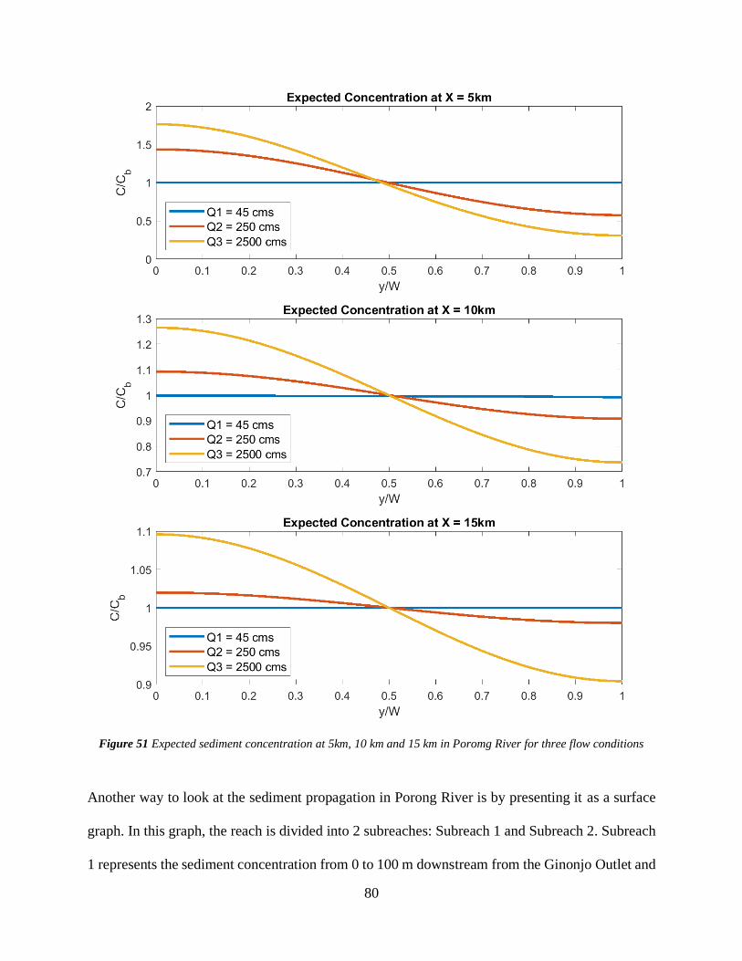
80
Figure 51 Expected sediment concentration at 5km, 10 km and 15 km in Poromg River for three flow conditions
Another way to look at the sediment propagation in Porong River is by presenting it as a surface
graph. In this graph, the reach is divided into 2 subreaches: Subreach 1 and Subreach 2. Subreach
1 represents the sediment concentration from 0 to 100 m downstream from the Ginonjo Outlet and

81
Subreach 2 represents the concentration from 100 m to the downstream end of the Porong River.
For the subreach 1 as presented in Figure 52, the trend of sediment propagation across the three
flow conditions was same, which they had a high sediment concentration at left bank and low
concentration at the right bank.
Because low flow condition has a low velocity, the diverted mud has more time to mix
transversally. This caused the concentration at 100 m downstream from the outlet at the left bank
side to decrease to about 2,000 mg/l, which equaled 3.5% of the initial concentration by the
diverted mud. The sediment concentration at the right bank side was 57 mg/l because the mud had
not reached that side. For medium flow, the sediment concentration at 100 m downstream from
the outlet at the left bank side was 800 mg/l, which equaled to 1.3% of the initial sediment
concentration. In the high flow condition, the sediment concentration at 100 m downstream from
the outlet at the left bank side was 150 mg/l, which was 0.2% of the initial concentration. We could
see that in the high flow condition, the sediment concentration at 100 m decrease 20 times more
dramatically than in low flow condition.
For the subreach 2 as depicted in Figure 53, the trend of sediment concentration in low flow
condition was different than the trend in medium and high flow condition. In low flow condition,
the diverted mud had fully-mixed transversally 4 km downstream from the outlet, which allowed
for a relatively identical sediment concentration in a cross-section beyond that point. The added
sediment concentration at 100 m downstream from the outlet was 2,000 mg/l and by the
downstream end of the Porong River was 475 mg/l. This means that there was a 76% loss of
sediment concentration in Subreach 2 for low flow condition. Meanwhile, medium flow and high
flow had a length scale of transversal mixing of 19 km and 29 km, respectively. These means that
a gradual reduction of sediment concentration was found moving downstream and laterally to the
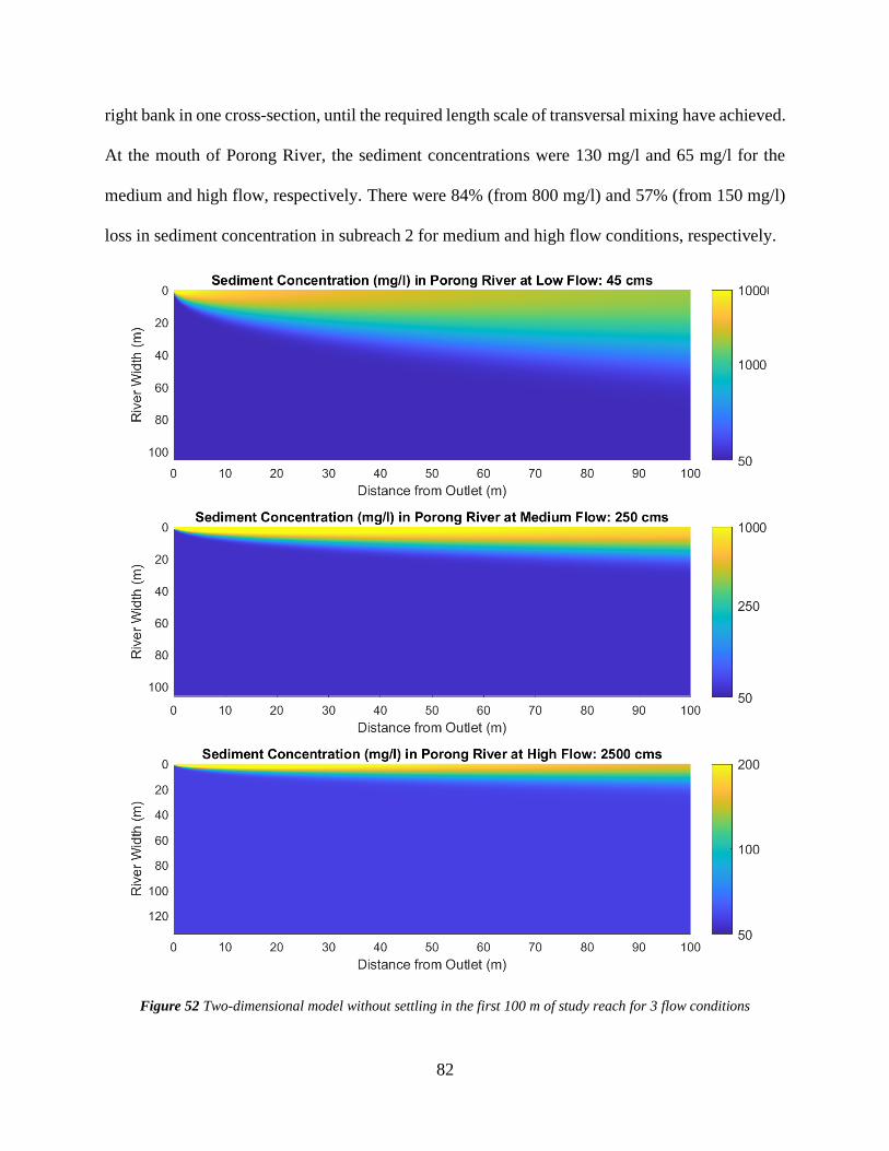
82
right bank in one cross-section, until the required length scale of transversal mixing have achieved.
At the mouth of Porong River, the sediment concentrations were 130 mg/l and 65 mg/l for the
medium and high flow, respectively. There were 84% (from 800 mg/l) and 57% (from 150 mg/l)
loss in sediment concentration in subreach 2 for medium and high flow conditions, respectively.
Figure 52 Two-dimensional model without settling in the first 100 m of study reach for 3 flow conditions

83
Figure 53 Two-dimensional model without settling from 100 m to 15800 m of study reach for 3 flow conditions
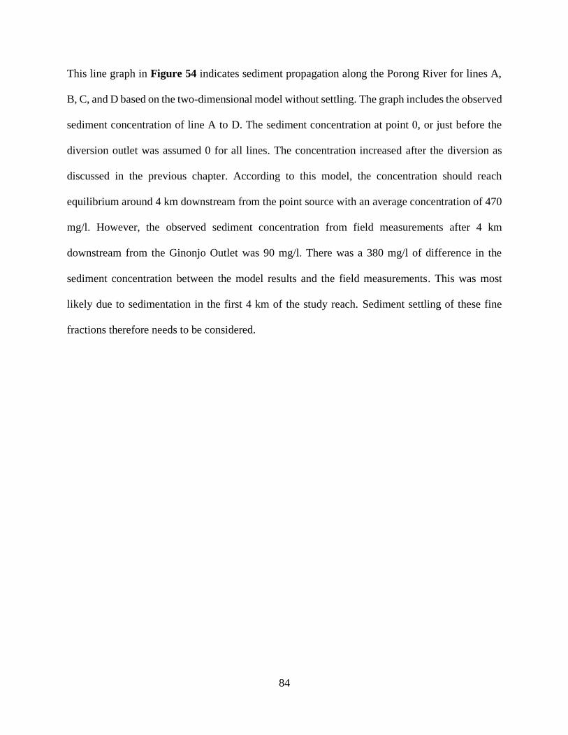
84
This line graph in Figure 54 indicates sediment propagation along the Porong River for lines A,
B, C, and D based on the two-dimensional model without settling. The graph includes the observed
sediment concentration of line A to D. The sediment concentration at point 0, or just before the
diversion outlet was assumed 0 for all lines. The concentration increased after the diversion as
discussed in the previous chapter. According to this model, the concentration should reach
equilibrium around 4 km downstream from the point source with an average concentration of 470
mg/l. However, the observed sediment concentration from field measurements after 4 km
downstream from the Ginonjo Outlet was 90 mg/l. There was a 380 mg/l of difference in the
sediment concentration between the model results and the field measurements. This was most
likely due to sedimentation in the first 4 km of the study reach. Sediment settling of these fine
fractions therefore needs to be considered.
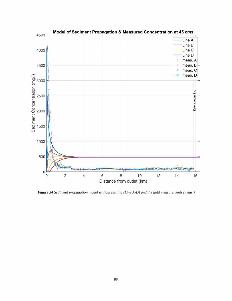
85
Figure 54 Sediment propagation model without settling (Line A-D) and the field measurements (meas.)
86
6.3 Two-Dimensional Mixing and Settling Model without Flocculation
Based on the analysis of the mud properties, it is clear that the diverted mud had a tendency to
flocculate and settle. In this case, the two-dimensional mixing model with finite width was not
adequate to predict the sediment propagation in the Porong River. Therefore, this research added
the settling factor into the two-dimensional mixing model. The settling factor comes from the
solution of advection-diffusion with nonconservative substance, which is:
𝑒−𝑘𝑖𝑡𝑗+1 =𝐶𝑖,𝑗+1
𝐶𝑖,𝑗
The 𝐶𝑖,𝑗+1 is the sediment concentration of fraction 𝑖 at location 𝑗 + 1, the 𝐶𝑖,𝑗 is the sediment
concentration of fraction 𝑖 at location 𝑗, the settling rate of fraction 𝑖, 𝑘𝑖 = 𝜔𝑖/ℎ, where 𝜔𝑖 is the
settling velocity of the fraction 𝑖 and ℎ is the flow depth. The time 𝑡 can be defined as 𝑋/𝑈, where
𝑋 is the river length and 𝑈 is the flow velocity.
Recall the two-dimensional mixing equation for finite width for equation at point 𝑗:
𝐶𝑗 = 𝐶𝑏
(
1
√4𝜋𝑥𝑗′
∑ {exp [−(𝑦′ − 2𝑛 − 𝑦0
′)2
4𝑥𝑗′ ] + exp [−
(𝑦′ − 2𝑛 + 𝑦0′)2
4𝑥𝑗′ ]}
∞
𝑛=−∞)
If we substitute the sediment concentration at point 𝑗, 𝐶𝑗, from the two-dimensional mixing
equation into the settling factor, we get:
𝐶𝑖,𝑗+1 = 𝐶𝑏,𝑖𝑒−𝑘𝑖𝑡𝑗+1
(
1
√4𝜋𝑥𝑗′
∑ {exp [−(𝑦′ − 2𝑛 − 𝑦0
′)2
4𝑥𝑗′ ] + exp [−
(𝑦′ − 2𝑛 + 𝑦0′)2
4𝑥𝑗′ ]}
∞
𝑛=−∞)
By utilizing this equation into our study, we can determine the sediment propagation in the Porong
River. Noted that the research computed the sediment concentration for every size fraction from

87
the particle size distribution to get a better understanding of the settled and unsettled portion of the
diverted mud. The total suspended sediment concentration is:
𝐶 =∑∆𝑝𝑖𝐶𝑖
where ∆𝑝𝑖 is the relative weight of fraction i and 𝐶𝑖 is the suspended sediment concentration for
fraction i.
The result of the model for Line A, the closest to the outlet, was compared to the maximum, mean,
and minimum values of the measured concentration as presented in Figure 55. However, the
measured concentration did not agree with the result from the model. The total sediment
concentration from the model at the downstream end of the Porong River was about 195 mg/l as
indicated by the cyan line. All of the big sediments, from 4.75 mm to 75 𝜇𝑚, settled at the first
200 m of the Porong River. The fraction of 13 𝜇𝑚 and 10 𝜇𝑚 mostly settled before 4 km of the
Porong River. The fraction of 7 𝜇𝑚 and 5 𝜇𝑚 mostly settled around 7 km and 15 km, respectively.
Only the fraction of 4 𝜇𝑚, 3 𝜇𝑚, and 1 𝜇𝑚 were in suspension util the downstream end of the
Porong River with concentration of 17 mg/l, 60 mg/l and 108 mg/l, respectively. Note that 8% of
the total sediment was the clay fraction. About half of the suspended fractions flocculated and
settled in the first 4 km.
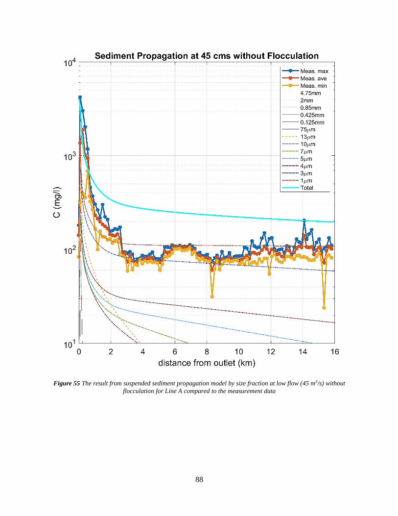
88
Figure 55 The result from suspended sediment propagation model by size fraction at low flow (45 m3/s) without
flocculation for Line A compared to the measurement data
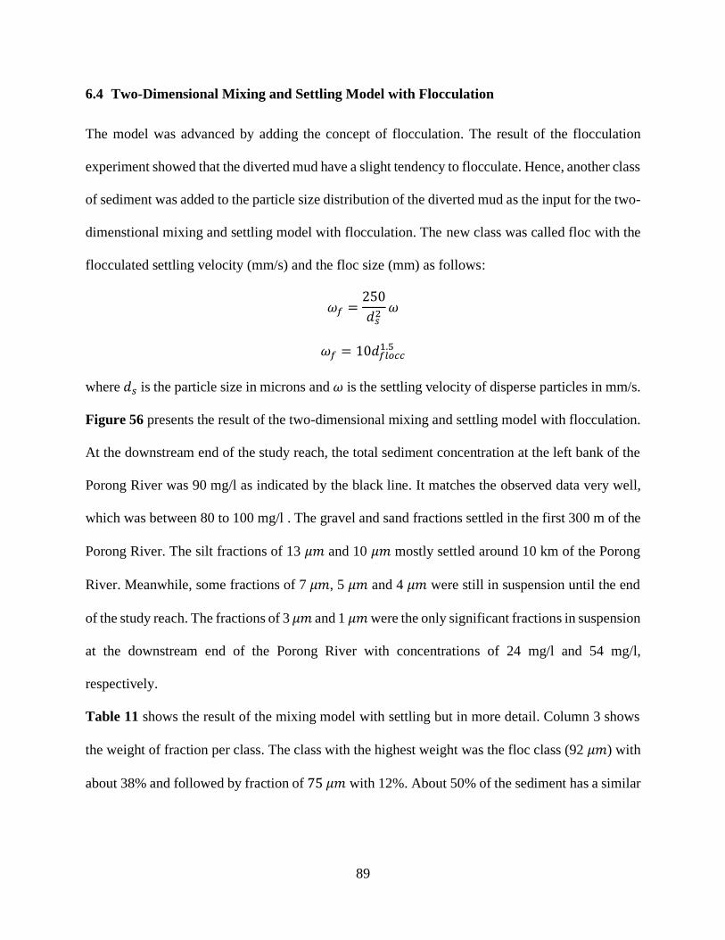
89
6.4 Two-Dimensional Mixing and Settling Model with Flocculation
The model was advanced by adding the concept of flocculation. The result of the flocculation
experiment showed that the diverted mud have a slight tendency to flocculate. Hence, another class
of sediment was added to the particle size distribution of the diverted mud as the input for the two-
dimenstional mixing and settling model with flocculation. The new class was called floc with the
flocculated settling velocity (mm/s) and the floc size (mm) as follows:
𝜔𝑓 =250
𝑑𝑠2𝜔
𝜔𝑓 = 10𝑑𝑓𝑙𝑜𝑐𝑐1.5
where 𝑑𝑠 is the particle size in microns and 𝜔 is the settling velocity of disperse particles in mm/s.
Figure 56 presents the result of the two-dimensional mixing and settling model with flocculation.
At the downstream end of the study reach, the total sediment concentration at the left bank of the
Porong River was 90 mg/l as indicated by the black line. It matches the observed data very well,
which was between 80 to 100 mg/l . The gravel and sand fractions settled in the first 300 m of the
Porong River. The silt fractions of 13 𝜇𝑚 and 10 𝜇𝑚 mostly settled around 10 km of the Porong
River. Meanwhile, some fractions of 7 𝜇𝑚, 5 𝜇𝑚 and 4 𝜇𝑚 were still in suspension until the end
of the study reach. The fractions of 3 𝜇𝑚 and 1 𝜇𝑚 were the only significant fractions in suspension
at the downstream end of the Porong River with concentrations of 24 mg/l and 54 mg/l,
respectively.
Table 11 shows the result of the mixing model with settling but in more detail. Column 3 shows
the weight of fraction per class. The class with the highest weight was the floc class (92 𝜇𝑚) with
about 38% and followed by fraction of 75 𝜇𝑚 with 12%. About 50% of the sediment has a similar

90
size with fine sand due to flocculation. Meanwhile, the clay fraction had been reduced to about
22% of the total sediment.
Figure 56 The result from suspended sediment propagation model by size fraction at low flow (45 m3/s) without
flocculation for Line A compared to the measurement data

Table 11 The classes of the diverted mud with its parameter and sediment concentration at certain distance from the Ginonjo Outlet
Class ds (mm)
dPi
(%)
(m/s) k
(1/s) C (mg/l) at X (m) =
0 100 300 500 1000 3000 5000 10000 15000 15800
1 4.75 0.9% 0.26 0.075 39 0 0 0 0 0 0 0 0 0
2 2 0.6% 0.17 0.048 23 0 0 0 0 0 0 0 0 0
3 0.85 0.6% 0.10 0.030 25 0 0 0 0 0 0 0 0 0
4 0.425 3.0% 0.06 0.019 123 0 0 0 0 0 0 0 0 0
5 0.125 6.0% 0.02 0.004 243 6 0 0 0 0 0 0 0 0
6 0.075 12.4% 0.01 0.002 505 117 2 0 0 0 0 0 0 0
7 0.013 8.3% 1.9E-04 5.5E-05 339 324 107 71 38 10 4 0 0 0
8 0.01 2.2% 1.1E-04 3.2E-05 91 89 30 21 12 5 3 1 0 0
9 0.007 2.6% 5.5E-05 1.6E-05 105 104 36 26 16 9 6 3 2 2
10 0.005 2.8% 2.8E-05 8.1E-06 114 113 40 29 19 11 10 7 5 5
11 0.004 2.7% 1.8E-05 5.2E-06 112 112 40 29 19 12 11 9 7 7
12 0.003 7.2% 1.0E-05 2.9E-06 294 293 105 76 51 33 31 27 24 24
13 0.001 11.7% 1.1E-06 3.2E-07 478 478 172 125 84 57 56 55 54 54
14 0.092 38.9% 2.8E-04 8.1E-05 1588 183 1 0 0 0 0 0 0 0
Total - 100% - - 4079 1819 535 376 240 138 120 102 92 91
91

92
As can be seen in Figure 57, the observed data were compared to the result from the two-
dimensional mixing and settling model with and without flocculation. The observed data, the
model with flocculation and the model without flocculation started at 4100 mg/l. For the most part
the sediment concentration of the model without flocculation at the left bank side was twice as
large as the sediment concentration of the model with flocculation, which was 90 mg/l. The
sediment concentration at the centerline and the right bank side started from very low and reached
their apex at 1 km with 150 mg/l and 2 km with 130 mg/l, respectively. After those point, the
sediment concentration kept decreasing until it became 90 mg/l. Furthermore, the percentage of
the sedimentation in the Porong River was calculatd by using the trap efficiency:
𝑇𝐸 =𝐶𝑗 − 𝐶𝑗+1
𝐶𝑗
The percentage of settled sediment in the Porong River in the low flow condition at the left bank
side was 98%, while at the centerline and the right bank side were 40% and 31%, respectively.
The presence of the mud diversion caused a higher sediment concentration in the Porong River.
The additional sediment concentration was very significant at the first 4 km downstream of the
diversion outlets and much lower by the end of the Porong River. Without any mud diversion, the
sediment concentration would be stagnant at about 50 mg/l based on the observed sediment
concentration upstream of the diversion outlets. Then, the observed data agreed with the two-
dimensional mixing and settling model with flocculation. It meant that the model can be used to
predict the sediment propagation in Porong River primarily because of the diversion from the mud
volcano.
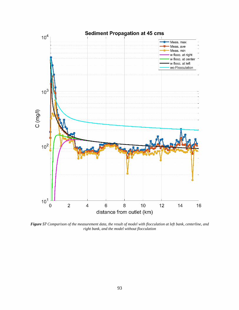
93
Figure 57 Comparison of the measurement data, the result of model with flocculation at left bank, centerline, and
right bank, and the model without flocculation

94
CHAPTER 7 MANAGEMENT
This chapter reviews some management issues and provides recommendations regarding the
disaster management of mud volcano.
7.1 Current Condition and Recommendation
7.1.1 Data availability and transparency
Historical data in water resources management field are very important. They are used to analyze
and to understand a particular past event or to foresee future scenarios. For example, a
comprehensive data set of river stages, discharges, cross-sections, infrastructures and ground
elevation of a city can be used to model and analyze the source of a flood event in the city. The
data are also useful to analyze the impact of future flood events.
One of the main problems in developing countries, particularly in Indonesia, is the data
availability and accessibility. The data are hardly available due to the limited instrumentation and
accessibility. Weather radars or stations are only available in urban areas. Meanwhile, a very
limited number of meteorological stations is installed in the wide mountain area which force the
researchers to extrapolate the data from the nearest point. It reduces the accuracy of model
predictions. Moreover, the weather stations or other instruments sometimes are not properly
maintained which caused an inability to record extreme events or missing some record data. One
of the great values of this dissertation is the effort to collect field measurements of sediment
concentration and turbidity at this site. The availability of discharge data at a national level should
facilitate future hydrologic and hydraulic studies. The access to topographic data, Digital Elevation
Models and LiDAR terrain data will also facilitate the future geo-spatial analysis of hydraulic and
sedimentation projects. Indonesia is a large and complex archipelago with a wide variety in altitude
and climatic conditions. Data transparency is another common problem in Indonesia. Because the

95
data are hard to collect, it becomes proprietory and difficult to access and share. At this time a
researcher sometimes needs to formally send a request letter or pay a certain fee for the data. Take
an example of a research of a flood control in a certain watershed. A researcher can download the
rainfall data in Indonesia from the Meteorogical, Climatological, and Geophysical Agency of
Indonesia (BMKG in Indonesian). However, for other data such as rating curve (river stages and
discharge), the researcher needs to send a request letter to a specific river basin organization who
manage the river. On the other hand, a dam structure is usually managed by other institution
than the river basin organization. Thus, the researcher has to send another letter to this institution
to get a record data of the dam. The request to these institutions will not be answered unless the
researchers have a good background or portfolio. This complicated institutional problem should
be solved to increase the effectiveness a research.
There are couple recommendations to solve or improve the data-availability and transparency
problem. A national program for data collection with public access would be a tremendous asset in
the future.
1. Installing a lot of new measurement instrument are essential to have a more comprehensive
data. As stated before, Indonesia needa many of rainfall or weather stations and the river
stations. The locations can be determine based on the long-term development plan. More
importantly, the installation sites should be able to cover the the critical watershed in the
water resources management plan in Indonesia. For example, the big city with high
frequency of flooding, are with major drought, irrigation land, the central for food
production, and the watershed of a dam structure.
2. Application of remote sensing measurement. This concept can be executed to collect a
water quality data. For example: to determine the total suspended solid in a river by using

96
a satellite data. The satellite data can be imported into water quality data through a specific
algorithm. In the early stage of the study, the result of the water quality data from the
remote sensing or predicted data should be validated by the field observation data. If the
deviations between the predicted data and the observed data are small, then the remote
sensing is accurate and the algorithm can be used for practical purpose. Furthermore,
remote sensing or remote measurement can be applied in the river monitoring field,
particularly to monitor the effluent from industry.
3. Technical and engineering data can be compiled in one government institution for external
request. The only access for students or researchers to collect data about the river should
be the river basin organization. The data include the properties of the river, plan view,
cross-sectional drawing, rating curve and the water quality data, including the dam
operation plan if there is any dam structure in the river. This could accelerate the data
collection step and encourage more research in water resources management or hydraulic
topics.
7.1.2 Mud Diversion
Based on the 15 years of experience with the mud diversion from the Sidoardjo Mud Volcano
and based on the result of the sediment propagation model, the mud diversion into the Porong
River will not clog the river. Furthermore, at the current diversion rates, it will not cause a massive
aggradation problem and flood to the surrounding area. The mud is dominated by fine sediment
which accounted for about 86% and most of the sediment will settle at the first 4 km. The
sediment deposited at low flow gets remobilized and transported to the estuary during floods.
Thus, the aggradation and degradation processes will balance each other.
The observed sediment propagation in the Porong River was collected manually by using a water

97
sampler. The shortcomings of the manual method are the required resources, such as man-power,
for the collection and the time to do the sample collection. In this research, the sample collection
was completed from 8AM to 5PM in more than 3 days. The unability to collect the sample at night
caused a discontinuation in observed data. To overcome this problem, a remote monitoring
can be installed and the data can be downloaded for several observation days. The strength of
the remote monitoring is the ability to collect a continuous data with a relatively cheaper
price than the conventional method.
One problem that occurred in the current mud diversion project is the measurement of sediment
concentration of the diverted mud. The sediment concentration is determined by using the
a hydrometer which is very inaccurate. A more accurate method to determine the sediment
concentration is by Total Suspended Solid (TSS) analysis in laboratory. A relationship between
the TSS analysis and the hydrometer analysis might be established for a practical use, but a more
detail research should be done regarding this relationship. One important contribution of this
dissertation has been the possibility to use turbidity measurements in correlation with sediment
concentration measurements. This turbidity versus concentration relationship may be helpful at
other similar sites in the future.
Another problem that can occur in the mud diversion phase is the contract of mud diversion
project. Due to the contract problem with the contractor, the mud diversion of the Sidoardjo Mud
Volcano had to be stopped for a couple months every year. Without a mud diversion, the
volume of mud inside the mud reservoir increased rapidly and endangered the stabilty of the
mud reservoir. This management issue can be solved by using a multi-year contract with
the contractor or the government can start the tender of the project before the end of the
current project. Another solution is the government divert the mud by themselves without the

98
help from contractor. This method gives a flexibility to the government to determine the
sediment concentration of the diverted mud. However, the government will need a skillful
staff and worker to execute the diversion.
7.2 Mud Volcano Disaster Guidelines
The Sidoardjo Mud Volcano is the first mud volcano that inflicted an urban area, in this case is
the Sidoardjo District. At the beginning of the eruption, the government did not have any
guidelines or policies to mitigate the damage of the Sidoardjo Mud Volcano. The mitigation action
was purely based on a trial and error basis with priority for human welfare. However, in
order to mitigate a huge social, economic, and environmental losses due to a mud volcano
disaster, a proper mitigation guidelines are essential. Thus, after decades of research
regarding the growth of the Sidaordjo Mud Volcano, including this research, proper
guidelines can be constructed.
The following are some proposed mud volcano disaster guidelines. Please note that the main
priority for these guidelines is human welfare.
1. The first step after the mud volcano is reported should be a preliminary study, which
includes the study of the characteristics of the mud volcano and the properties of the mud
sediment. In this preliminary study, the chamber and the source of the extruded mud, the
volume of extruded mud, the longevity of the mud volcano, and the subsidence area can be
studied and predicted for the basis of the mud volcano disaster policy. The preliminary
study should be finished in 2 to 3 months. In the meantime, the government can start to
relocate the neighborhood in the radius of 0.5 km from the main crater.
99
2. The second step is securing the affected zone of the mud volcano by land acquisition and
creating a mud reservoir. The affected zone include the required land for the mud reservoir,
which is based on the volume prediction of the extruded mud with a sufficient
embankment, and the subsidence area. The government have to complete the construction
of the reservoir in 6 months. This might be hard, but the construction can be divided into
several phases based on the total affected zone. The first phase is the land acquisition and
constuction of the inner mud reservoir which should be done in less than 2 weeks. The
second phase is for the middle reservoir which can be constructed in 2 months and the third
phase is for the outer reservoir with a construction time of 3 months. The design of the mud
reservoir must consider the mud flow movement inside the reservoir and the mud diversion
plan. At this step, the number of refugees should be finalized as the affected zone have
been implemented and the social problem should be solved.
3. The third step is initiating the mud diversion to an ocean through the nearest possible river.
A feasibility study is important to look for the most effective and efficient procedure to
divert the mud. The study includes the physical and chemical properties of the mud, the
bathymetri of the river, the maximum allowable diverted mud into the river, the possible
aggradation and degradation of the river, and the sediment transport of the river. Moreover,
the sediment propagation of the diverted mud in the river should be modeled to get a better
understanding about the sediment transport in the river.
4. The fourth step is river monitoring. It could be completed daily or, at least, weekly in order
to maintain and prevent any future damage to the river. The monitoring includes the river
discharge, the particle size distribution of the diverted mud, the sediment concentration of
the diverted mud, the aggradation and degradation of the river bed, the sediment

100
propagation, and the sedimentation at the estuary. The weekly monitoring is important
because the particle size and sediment concentration of the diverted mud are changing in
daily basis.
Nowadays, many mud volcanoes are still springing up on the Java and across the globe.
Sometimes, it appears inside a house but only lasts a couple of hours. However, a mud volcano
similar to the Sidoardjo Mud Volcano can occur again in the future, maybe in Indonesia or
elsewhere around the world. Thus, a document providing guidelines for managing mud
volcanoes is urgently needed to give a better framework to mitigate the damage of a mud
volcano to the human welfare.
101
CHAPTER 8 CONCLUSIONS
This research addresses an interesting issue in the field of civil and environmental engineering;
namely the impact of diverting large flows of mud from the point source to the downstream 16 km
of the Porong River towards an open strait. Using the Sidoarjo Mud Volcano eruption as a case
study, this research has attempted to answer several scientific questions as stated in the Chapter 1.
To this end, the research has analyzed the dynamics of sediment propagation along the Porong
River. These actions have been done through analysis and through field measurement programs
that were used to test the computational model and establish sediment concentration data sets. By
completing this research, the idea of diverting the mud from the mud volcano into the Porong River
will not cause any major disturbance to the river. It works well to reduce the volume of the mud
inside the mud reservoir and the aggradation – degradation processes are balancing each other.
8.1 Properties of the Diverted Mud
a. The results of the particle size distribution analysis were: the median particle size of the
extruded mud, Pejarakan’s diverted mud, and Ginonjo’s diverted mud were 8 𝜇𝑚, 3.4 𝜇𝑚,
and 4.7 𝜇𝑚, respectively.
Laboratory experiments were conducted on July 5, 2019 on the soil sample from the
Sidoardjo mud volcano. The experiments of turbidity and sediment concentration
concluded that the linear regression, 𝐶 = 5.297 × 𝑇𝑢𝑟 + 23.96, was the best fitted
regression with coefficient of determination 𝑟2 = 0.99.
b. Flocculation tests using deflocculant agents, sodium hexametaphosphate and sodium
carbonate, were completed in 2019. For the samples from Ginonjo Outlet, the recorded
deflocculated settling velocity was 0.013 mm/s which was 2 times slower than the natural
settling velocity of 0.028 mm/s. This value was one order slower than the general settling
102
velocity for flocculated particles which is between 0.15 to 0.6 mm/s. The test concluded
that the mud has a slight tendency to flocculate.
8.2 Field Measurements
a. Field Measurement Program #1 was conducted at 106 cross-sections with 150 m distance
between each cross-section, covering16 km of the Porong River to measure sediment
concentration. There were 4 points of measurement in each cross-section with 25 m
distance between each point and 5 m offset from the left and right bank. The highest
sediment concentration should be higher at the left bank of the Porong River. However, the
maximum observed sediment concentration for each line was located at cross-section 2 (80
m downstream from the Ginonjo Outlet) was 4,198 mg/l at line C, 2,704 mg/l at line D,
2,021 mg/l at line B, and 691 mg/l at line A. It means that the lateral mixing is much larger
along the first 4 km of the study reach. It might ce caused by the river bed protection
immediately downstream from the Ginonjo Outlet.
b. Field Measurement Program #2 was conducted to capture the vertical sediment
concentration profiles for the first 4km and to look into possible flocculations. The water
was collected at every 1 m in depth. Total number of samples were 307 bottles. The highest
near-bed sediment concentration was 1,500 mg/l at Line C cross-section 9, followed by
1,450 mg/l at Line C cross-section 6. The results of Field Measurement Program #2 shows
that the sediment concentration are uniform along the Porong River except for the first 4
km where the bottom sediment concentration is high.
8.3 Sediment Propagation Model for Porong River
a. HEC-RAS was used to calculate the hydraulic properties of the Porong River, such as the
flow depth, width and average velocity. Three flow conditions based on the hydrograph of

103
the Porong River were defined: low flow with 45 m3/s, medium flow with 250 m3/s, and
high flow with 2500 m3/s. For low flow condition, the average flow velocity was 0.12 m/s,
the average flow depth was 3.5 m, the top width was 105 m, the energy slope was 0.3
cm/km and the shear velocity was 0.01 m/s. The simulation was done from January 2012
to December 2016. No significant bed change was observed along the simulation time.
b. Sediment concentration of the diverted mud at Ginonjo Outlet was 57,000 mg/l. The results
of the mixing model without settling show that the fully-mixed concentration for low flow
condition (45 m3/s) were achieved at 4 km downstream from the outlet with a concentration
of 470 mg/l. However, the average observed sediment concentration was about 90 mg/l
and the sediment concentration difference was 380 mg/l.
c. The two-dimensional mixing and setting model without flocculation was used by applying
the settling factor into the mixing model with finite width. The gravel, sand, and coarser
silt fractions were settled in the first 4 k m of the study reach while the finer silt fraction
was settled at 7 km. Only the clay fraction was in suspension by the end of study reach
with the sediment concentration of 195 mg/l. The clay fraction was accounted for about
48% of the total sediment. The sediment concentration difference between this model and
observed data is 105 mg/l.
d. The two-dimensional mixing and setting model with flocculation was then used to advance
the previous model. The sediment concentration at the left bank of the Porong River was
about 90 mg/l, which matched the observed data. The gravel, sand, and coarser silt fractions
settled along the first 4 k m of the study reach, including the flocculated particle with a size
of 92 𝜇𝑚. Only clay fraction were in suspension by the end of study reach with a

104
concentration of 24 mg/l and 54 mg/l, respectively. The flocculated particle accounted for
38% of the total sediment while the clay particle reduced to about 22%.
8.4 Mud Volcano Disaster Guidelines
a. The idea of diverting mud into the Porong River will not cause any damage to the river
because the aggradation will occur in the rainy season and degradation will occur in dry
season. The diversion works well to reduce the volume of sediment insdie the mud
reservoir.
b. The current problem on mud diversion work in the Sidoardjo Mud Volcano, and generally
in Indonesia, includes the data availability and data transparency. These problems can be
solved with sheer effort from the government and the private sector by installing many new
measurement instruments.
c. A guidelines for the future mud volcano disaster has been established with the priority for
the human welfare. It is based on the technical findings in and recommendation of this
thesis. It includes the preliminary study, securing the affecting zone for mud reservoir, mud
diversion work, and the river monitoring.
105
BIBLIOGRAPHY
Aboubakr, S., Reda Taha, M. M., and Kandil, U. (2013) Creep of epoxy-clay nanocompsite at FRP
interface. Ninth International Conference of Composite Science and Technology, ICCST 9.
Akalin, S. (2002). Water temperature effect on sand transport by size fraction in the lower
Mississippi River. Ph.D. dissertation, Colorado State University.
Allen, G. P., Salomon, J. C., Bassoullet, P., Penhoat, Y. D., and Grandpre, C. D. Effect of tides on
mixing and suspended sediment transport in microtidal estuaries. Sedimentary Geology, 26, p.
69-90.
Aniekan, E. I., Ebunilo, P. O., and Okovido, J. (2018). Geotechnical evaluation of bentonite clay
for municipal solid waste landfill lining membrane. J. Envir. Eng. Sci. 4, p. 337-351.
Aris, R. (1956). On the dispersion of a solute in a fluid flowing through a tube. Proceeding of the
Royal Society of London. Series A. Mathematical and Physical Sciences.
Armijos, E., Crave, A., Espinoza, R., Fraizy, P., Dos Santos, A. L. M. R., Sampalo, F., De Oliveira,
E., Santini, W., Martinez, J. M., Autin, P., Pantoja, N, Oliveira, M., and Filizola, N. (2017).
Measuring and modeling vertical gradients in suspended sediments in the Solimões/Amazon
River. Hydrological Processes, 31, p. 654-667.
Bioresita, F., Pribadi, C. B., Firdaus, H. S., Hariyanto, T., and Puissant, A. (2018). The use of
Sentinel-2 imagery for total suspended solids (TSS) estimation in Porong River, Sidoardjo.
Elipsoida: Jurnal Geodesi dan Geomatika, vol. 01, no. 01, p. 1-6.
Blouin, A., Imbert, P., Sultan, N. and Callot, J.-P. (2019). Evolution model for the Absheron Mud
Volcano: from in situ observations to numerical modeling. Journal of Geophysical Research:
Earth Surface, 124, p. 766-794.

106
Brandon, C. D., and Karathanasis, A.D. (2002). Clay minerals. Encyclopedia of Soil Science, p.
187-192.
Breen, N. A., Silver, E. A., and Hussong, D. M. (1986). Structural styles of an accretionary wedge
south of the island of Sumba, Indonesia, revealed by SeaMARC II side scan sonar. Geological
Society of America Bulletin, v. 97, p. 1250-1261.
Brunner, G. W. (2016). HEC-RAS, river analysis system hydraulic reference manual. US Army
Corps of Engineers Hydrologic Engineering Center (HEC). California: Davis.
Chapra, S. C. (1997). Surface Water-Quality Modeling. USA: McGraw-Hill.
Cheng, N-S. (1997). Effect of concentration on settling velocity of sediment particles. Journal of
Hydraul. Engineering, vol. 128, p. 728-731.
Chow, V.T. (1959). Open-Channel Hydraulics. New Jersey: The Blackburn Press.
Christensen, V. G., Rasmussen, P. P., and Ziegler, A. C. (2002). Comparison of estimated sediment
loads using continuous turbidity measurements and regression analysis. Turbidity and Other
Surrogates Workshop.
Cody, C. A., and Magauran, E. D. (1990). Method of treating waste water for organic
contaminants with water dispersible organically modified smectite clay compositions,
US5130028A.
Daphne, L. H. X., Utomo, H. D., and Kenneth, L. Z. H. (2011). Correlation between Turbidity and
Total Suspended Solids in Singapore Rivers. Journal of Water Sustainability, vol. 1, Issue 3.
Davies, R. J., Mathias, S. A., Swarbrick, R. E., and Tingay, M. J. (2011). Probabilistic longevity
estimate for the LUSI mud volcano, East Java. Journal of Geological Society, vol. 168, p. 517-
523.

107
Davies, R. J., Swarbrick, R. E., Evans, R. J., and Huuse, M. (2007). Birth of a mud volcano: East
Java, 29 May 2006. GSA Today, v. 17, no. 2, p. 4-9.
Davies, R., Manga, M., Tingay, M., Lusianga, S., and Swarbrick, R. (2010). Sawolo et al. (2009)
the Lusi mud volcano controversy: Was it caused by drilling? Marine and Petroleum Geology,
v. 27, p. 1651-1657.
Dimitrov, L. I. (2002). Mud volcanoes – the most important pathway for degassing deeply buried
sediments. Earth-Science Reviews, 59, 49-76.
Ettema, R. (2006). Hunter Rouse – His work in retrospect. J. Hydraul. Eng., 132, 1248-1258.
Fischer, H. B., List, E. J, Koh, R. C. Y., Imberger, J., and Brooks, N. H. (1979). Mixing in inland
and coastal waters. New York: Academic Press, Inc.
Foster, I. D. L., Millington, R., and Grew, R. G. (1992). The impact of particle size controls on
stream turbidity measurement; some implications for suspended sediment yield estimation.
Erosion and Sediment Transport Monitoring Programmes in River Basin (Proceedings of the
Oslo Symposium). IAHS Publ. no. 210, p. 51-62.
Geospatial Information Agency. (2019). Online tidal prediction. Retrieved from:
http://tides.big.go.id/pasut/index.html
Gippel, C. J. (1989). The use of turbidimeters in suspended sediment research. Hydrobiologia
176/177, p. 465-480.
Gujarati, D. N., Porter, D. C., and Gunasekar, S. (2012). Basic Econometrics (5th ed.). Tamil Nadu:
McGraw Hill Education (India) Private Limited.
Guo, C., He, Q., Guo, L., and Winterwerp, J. C. (2017) A study of in-situ sediment flocculation in
the turbidity maxima of the Yangtze Estuary. Estuarine, Coastal and Shelf Science, vol. 191,
p. 1-9.
108
Guy, H. P. (1969). Laboratory theory and methods for sediment analysis. United States Geological
Survey Techniques of Water Resources Investigations, Book 5.
Hadimuljono, M. B. (2008). Sidoardjo’s Hot Mudflow Catastrophe: Lessons from a Disaster.
Hamilton, L. J., Shi, Z., and Zhang, S. Y. (1998). Acoustic backscatter measurements of estuarine
suspended cohesive sediment concentration profiles. Journal of Coastal Research, 14, p. 1213-
1224.
Harnanto, A. (2011). Peranan Kali Porong dalam mengalirkan lumpur Sidoardjo ke laut. Badan
Pelaksana – Badan Penanggulangan Lumpur Sidoarjo (BAPEL-BPLS).
Hermawan, C. (2012). Debit minimum Kali Porong untuk menjamin angkutan sedimen sampai ke
muara Kali Porong (Bachelor Thesis). Retrieved from digilib.uns.ac.id.
Hernawan, U., and Budiono, K. (2012). Karakteristik dan distribusi lumpur Sidoardjo sepanjang
sungai, estuary dan perairan Porong. Jurnal Geologi Kelautan, vol 11, no 2, p. 91-100.
Hidayati, D., Sulaiman, N., Ismail, B. S., Shuhaimi-Othman, M., and De Bellard, M. E. (2017).
Evaluation of the effect of Sidoardjo Mud on aquatic life using chromatophores and the
microstructure of fish scales. Sains Malaysiana, 46(3), p. 373-380.
Hoekstra, P. (1988). Hydrodynamics and depositional processes of the Solo and Porong Deltas,
East Java, Indonesia. Proceedings KNGMG Symposium ‘Coastal Lowlands, Geology and
Geotechnology’, p. 161-173.
Holliday, C. P., Rasmussen, T. C., and Miller, W. P. (2003). Establishing the relationship between
turbidity and total suspended sediment concentration. Proceedings of the 2003 Georgia Water
Resources Conference, April 23-24, 2003. Athens, Georgia.
Hunt, J. N. (1954) The turbulent transport of suspended sediment in open channels. Proc., Royal
Society, 224, p. 322-335.
109
Indonesian Government. (2001). Peraturan Pemerintah Republik Indonesia Nomor 82 Tahun
2001 tentang Pengelolaan Kualitas Air dan Pengendalian Pencemaran Air. Jakarta: State
Secretariat.
Indrawan, D., Chayono, M., and Moerwanto, A. S. (2013). Analisis gerak mula pertikel sedimen
kohesif (studi kasus lumpur Lapindo Sungai Porong). Jurnal Teknik Hidraulik, vol 4, no 1, p.
39-50.
International Organization for Standardization. (2016). Water quality – determination of turbidity
– part 1: quantitative methods. ISO 7027-1.
Istadi, B. P., Pramono, G. H., Sumintadireja, P., and Alam, S. (2009). Modeling study of growth
and potential geohazard for LUSI mud volcano: East Java, Indonesia. Marine and Petroleum
Geology, 26, p. 1724-1739.
Jansson, M. B. (1992). Turbidimeter measurements in a tropical river, Costa Rica. Erosion and
Sediment Transport Monitoring Programmes in River Basin (Proceedings of the Oslo
Symposium). IAHS Publ. no. 210, p. 71-78.
Jennerjahn, T. C., Jänen, T., Propp, C., Adi, S., and Nugroho, S. P. (2013). Environmental impact
of mud volcano inputs on the anthropogenically altered Porong River and Madura Strait coastal
waters, Java, Indonesia. Estuarine, Coastal and Shelf Science, 130, p. 152-160.
Julien, P. Y. (2010). Erosion and sedimentation (2nd ed.). New York: Cambridge University Press.
Julien, P. Y. (2018). River Mechanics. New York: Cambridge University Press.
Julien, P. Y., and Mendelsberg, A. (2003). Sediment in Arroyo Pasajero and San Luis Canal.
Report. Dept. of Civil Engineering. Colorado State University.
Jung, S. H., Seo, I. W., Kim, Y. D., and Park, I. (2019). Feasibility of velocity-based method for
transverse mixing coefficients in river mixing analysis. J. Hydraul. Eng., 145.
110
Kineke, G. C., and Sternberg, R. W. (1989). The effect of particle settling velocity on computed
suspended sediment concentration profiles. Marine Geology, 90, p. 159-174.
Kociuba, W. (2017). Determination of the bedload transport rate in a small proglacial High Arctic
stream using direct, semi-continuous measurement. Geomorphology, 287, p. 101-115.
Kopf, A. J. (2002). Significance of mud volcanism. Rev. Geophys., 40(2), 1005.
Kure, S., Winarta, B., Takeda, Y., Udo, K., Umeda, M., Mano, A., and Tanaka, H. (2014). Effects
of mud flows from the LUSI mud volcano on the Porong River estuary, Indonesia. Journal of
Coastal Research, 70, p. 568-573.
Laboratorium Mekanika Tanah dan Batuan. (2018) Laporan hasil uji analisa pembagian butir.
Institut Teknologi Sepuluh November – Fakultas Teknik Sipil dan Lingkungan.
Laboratorium Transportasi dan Geoteknik. (2018). Laporan hasil tes laboratorium PPLS (Pusat
Pengendalian Lumpur Sidoardjo). Intitut Teknologi Sepuluh November – Fakultas Vokasi.
Lewis, J. (1996). Turbidity-controlled suspended sediment sampling for runoff-event load
estimation. Water Resources Research, vol. 32, no. 7, p. 2299-2310.
Lupi, M., Saenger, E. H., Fuchs, F., and Miller, S. A. (2013). Lusi mud eruption triggered by
geometric focusing of seismic waves. Nature Geoscience, vol. 6, p. 642-646.
Manga, M. (2007). Did an earthquake trigger the May 2006 eruption of the Lusi mud volcano?
Eos, vol. 88, p. 201.
Manga, M., Brumm, M., and Rudolph, M. L. (2009). Earthquake triggering of mud volcanoes.
Marine and Petroleum Geology, vol. 26, p. 1785-1798.
Marchuk, S. (2016). The Dynamics of potassium in some Australian soils. Ph.D. Dissertation, The
University of Adelaide.

111
Mazumder, B. S., and Ghoshal, K. (2006). Velocity and concentration profiles in uniform
sediment-laden flow. Applied Mathematical Modelling, 30, p. 164-176
Mazzini, A., Svensen, H., Akhmanov, G. G., Aloisi, G., Planke, S., Malthe-Sørenssen, A., and
Istadi, B. (2007). Triggering and dynamic evolution of the LUSI mud volcano, Indonesia.
Earth and Planetary Science Letters, 261, p. 375-388.
McCarthy, J. C., Pyle, T. E., and Griffin, G. M. (1974). Light transmissivity, suspended sediments
and legal definition of turbidity. Estuarine and Coastal Marine Science 2, p. 291-299.
McMichael, H. (2009). The Lapindo mudflow disaster: environmental, infrastructure and
economic impact. Bulletin of Indonesian Economic Studies, 45(1), p. 73-83.
Mellors, R., Kilb, D., Aliyev, A., Gasanov, A., and Yetirmishli, G. (2007). Correlations between
earthquakes and large mud volcano eruptions. J. Geophys. Res., 112, B04304.
Meyer-Peter, E., and Muller, R. (1948). Formulas for bed-load transport. Proc. 2nd Meeting IAHR,
Stockholm, p. 39-64.
Migniot, C. (1989). Tassement et rheologie des vases. La Houille Blanche, no. 1, p. 11-29.
Milkov, A. V. (2000). Worldwide distribution of submarine mud volcanoes and associated gas
hydrates. Marine Geology, 167, p. 29-42.
Minella, J. P. G., Merten, G. H., Reichert, J. M., and Clarke, R. T. (2008). Estimating suspended
sediment concentrations from turbidity measurements and the calibration problem.
Hydrological Processes 22, p. 1819-1830.
Mori, J., and Kano, Y. (2009). Is the 2006 Yogyakarta earthquake related to the triggering of the
Sidoardjo, Indonesia mud volcano? Journal of Geography, vol. 118(3), p. 492-498.
112
Ndolo Goy, P. (2015). GIS-based soil erosion modeling and sediment yield of the N’djili River
Basin, Democratic Republic of Congo (Masters Thesis). Retrieved from
https://www.engr.colostate.edu/~pierre/
Ni, J. R., and Wang, G. Q. (1991). Vertical sediment distribution. J. Hydraul. Eng., 117, p.1184-
1194.
O’Loughlin, E. M., and Bowmer, K. H. (1975). Dilution and decay of aquatic herbicides in flowing
channels. Journal of Hydrology, 26, p. 217-235.
Odom, I. E. (1984). Smectite clay minerals: properties and uses. Trans. R. Soc. Lond., A 311,
p.391-409.
Pahlevi, A. M., and Wiweka. (2010). Analisa sedimentasi di muara Kali Porong akibat
pembuangan lumpur Lapindo menggunakan data citra satelit ASTER. Jurnal Ilmiah
Geomatika, vol 16, no 2, p. 23-42.
Palu, M. (2019). Floodwave and sediment transport assessment aling the Doce River after the
Fundao Tailings Dam collapse (Brazil). (Ph.D. Dissertation). Retrieved from
https://www.engr.colostate.edu/~pierre/
Palu, M. C., Julien, P. Y. (2019). Modeling the sediment load of the Doce River after the Fundao
Tailing Dam collapse, Brazil. J. Hydraul. Eng., 145.
Pavanelli, D., and Bigi, A. (2005). Indirect methods to estimate suspended sediment concentration:
reliability and relationship of turbidity and settleable solids. Biosystems Engineering 90(1), p.
75-83.
Pejrup, M., and Mikkelsen, O. A. (2009). Factors controlling the field settling velocity of cohesive
sediment in estuaries. Estuarine, Coastal and Shelf Science, vol. 87, p. 177-185.
113
Pfannkuche, J., and Schmidt A. (2003). Determination of suspended particulate matter
concentration from turbidity measurements: particle size effects and calibration procedures.
Hydrological Processes 17, p. 1951-1963.
Plumlee, G. S., Casadevall, T. J., Wibowo, H. T., Rosenbauer, R. J., Johnson, C. A., Breit, G. N.,
Lowers, H. A., Wolf, R. E., Hageman, P. L., Goldstein, H., Anthony, M. W., Berry, C. J., Fey,
D. J., Meeker, G. P., and Morman, S. A. (2008). Preliminary analytical results for a mud
sample collected from the LUSI mud volcano, Sidoardjo, East Java, Indonesia. USGS.
Reichert, J. M., Norton, L. D., Favaretto, N., Huang C., and Blume, E. (2009). Settling velocity,
aggregate stability, and interrill erodibility of soils varying in clay mineralogy. Soil Sci. Soc.
Am. J., vol. 73, p. 1369-1377.
Riley, S. J. (1998). The sediment concentration – turbidity relation: its values in monitoring at
Ranger Uranium Mine, Northern Territory, Australia. Catena 32, p. 1-14.
Rouse, H. (1937). Modern conception of the mechanics of turbulence. Trans. ASCE, 102, p 463-
543.
Rudolph, M. L., Karlstrom, L., and Manga, M. (2011). A prediction of the longevity of the Lusi
mud eruption, Indonesia. Earth and Planetary Science Letters, 308, p. 124-130.
Sasaki, Y. and Yamamoto, O. (2017). Bacterial adsorption effect of smectite for wound-healing
application. Journal of the Ceramic Society of Japan, 125 [9], p. 710-712.
Satyana, A. H., and Asnidar (2008). Mud diapirs and mud volcanoes in depressions of Java to
Madura: origins, nature, and implications to petroleum system. Proceedings, Indonesian
Petroleum Association Thirty-Second Annual Convention and Exhibition.

114
Sawolo, N., Sutriono, E., Istadi, B. P., and Darmoyo, A. B. (2009). The LUSI mud volcano
triggering controversy: Was it caused by drilling?, Marine and Petroleum Geology, 26, p.
1766-1784.
Sawolo, N., Sutriono, E., Istadi, B. P., and Darmoyo, A. B. (2010). Was Lusi caused by drilling?
– Authors reply to discussion. Marine and Petroleum Geology, vol. 27, p. 1658-1675.
Shah-Fairbank, S. C., Julien, P. Y., and Baird, D. C. (2011). Total sediment load from SEMEP
using depth-integrated concentration measurements. J. Hydraul. Eng., p. 1606-1614.
Shen, Y., Zhu, Y., Ge, D., and Shen, X. (2016). Effects of initial concentration on flocculation size
and settling velocity of marine hydraulic fill clay. Thalasssas, 32, p. 117-122.
Shi, J. Z. (2010). Tidal resuspension and transport processes of fine sediment within the river
plume in the partuakky-mixed Changjian River estuary, China: A personal perspective.
Geomorphology, 121, p. 133-151.
Shirzaei, M., Rudolph, M. L., and Manga, M. (2015). Deep and shallow sources for the Lusi mud
eruption revealed by surface deformation. Geophysical Research Letters, vol. 42, p. 5274-
5281.
Silver, E. A., Breen, N. A., and Prasetyo, H. (1986). Multibeam study of the Flores backarc thrust
belt, Indonesia. Journal of Geophysical Research, vol. 91, no. B3, p. 3489-3500.
Suntoyo, Ikhwani, H., Zikra, M., Sukmasari, N. A., Angraeni, G., Tanaka, H., Umeda, M., and
Kure, S. (2015). Modelling the COD,TSS, Phosphate and Nitrate distribution due to the
Sidoardjo Mud Flow into Porong River estuary. Procedia Earth and Planetary Science 14, p.
144-151.
Sutherland, B. R., Barrett, K. J., and Gingras, M. K. (2014). Clay settling in fresh and salt water.
Environmental Fluid Mechanics, vol. 15. P. 147-160.

115
Tanaka, S., and Sugimoto, S. (1958). On the distribution of suspended sediment in experimental
flume flow. Memoirs of the Faculty of Engineering, Kobe University.
Tingay, M., Heidbach, O., Davies, R., and Swarbrick, R. (2008). Triggering of the Lusi mud
eruption: Earthquake versus drilling initiation. Geology, vol. 36, no. 8, p. 639-642.
Tingay, M. R. P., Rudolph, M. L., Manga, M., Davies, R. J., and Wang, C. (2015). Initaition of
the Lusi mudflow disaster. Nature Geoscience, vol. 8, p. 493-494.
Usman, E., Salahuddin, M., Ranawijaya, DAS., and Hutagaol, J. P. (2016). Lokasi pengendapan
akhir dan evaluasi pengelolaan lumpur Porong. Retrieved Feb 19, 2018.
www.mgi.esdm.go.id/content/lokasi-pengendapan-akhir-dan-evaluasi-pengelolaan-lumpur-
porong.
van Rijn, L. C. (1984a). Sediment transport, Part I: Bed load transport. J. Hydraul. Eng., 110, p.
1431-1456.
van Rijn, L. C. (1984b). Sediment transport, Part II: Suspended load transport. J. Hydraul. Eng.,
110, p. 1613-1641.
Vanoni, V. A. (1962). Sedimentation Engineering – ASCE Manual and Reports on Engineering
Practice No. 54 (Reprinted 1977).
Vercruysse, K., Grabowski, R. C., and Rickson, R.J. (2017). Suspended sediment transport
dynamics in rivers: Multi-scale drivers of temporal variation. Eath-Science Reviews, 166, p.
38-52.
Williams, P. R., Pigram, C. J., and Dow, D. B. (1984). Melange production and the importance of
shale diapirsm in accretionary terrains. Nature, vol. 309, p. 145-146.
Winterwerp, H. (1999). On the dynamics of high-concentrated mud suspensions. Report. Dept. of
Civil Engineering and Geosciences. Delft University of Technology.
116
Wren, D. G., Barkdoll, B. D., Kuhnle, R. A., and Derrow, R. W. (2000). Field techniques for
suspended-sediment measurement. J. Hydraul. Eng., 126, p. 97-104.
Yang, C. T., Molinas, A., and Wu, B. (1996). Sediment transport in the Yellow River. J. Hydraul.
Eng., 122, p. 237-244.
Zhu, H. W., Cheng, P. D., Li, W., Chen, J. H., Pang, Y., and Wang, D. Z. (2017). Empirical model
for estimating vertical concentration profiles of re-suspended, sediment-associated
contaminants. Acta Mech. Sin., 33, p. 846-854.

117
APPENDIX A
Laboratory experiment of the relationship between the turbidity and sediment concentration.
The laboratory experiment procedures were:
1. Prepare a 0.5 gram of sediment from the mud reservoir in a glass beaker. Use the balance
to accurately prepare the sediment sample.
2. Collect 100 ml Porong River water in the flask, then add it into the sediment sample.
3. Record the sediment concentration (mg/l) and turbidity (NTU) by using the turbidimeter.
Do at least 2 turbidity measurements for each corresponding concentration.
4. Add 100 ml Porong River water to decrease the sediment concentration of the mixture and
record the sediment concentration and the turbitiy.
5. Repeat step 4 until the turbidity of our mixture remains unchanged or until the mixture is
clearer than the water condition in the Porong River.
Error analysis for the relationship of turbidity and sediment concentration.
We would focus on the linear regression as the best fitted regression and power regression for a
comparison with the linear regression. The error of regression could be analyzed by using residual
plot. Residual 𝑒 is the difference between the observed or actual value 𝑦 and predicted or estimated
value �̂� (Gujarati, 2012), such as,
𝑒 = 𝑦 − �̂� (32)
where the observed sediment concentration data were used as the actual value 𝑦 and the predicted
values �̂� come from the regression analysis by applying the turbidity data set 2.
Figure 58 presents the residual plot for the relationship of turbidity and sediment concentration in
the Porong River for linear and power regression. The linear regression gains the highest residual

118
as −195.9 𝑚𝑔/𝑙, followed by 184.1 𝑚𝑔/𝑙. Note that negative value in residual means an
overestimated value of dependent variable or sediment concentration in this case while positive
value means an underestimated value of sediment concentration. The power regression shows that
the highest residual is −724.9 𝑚𝑔/𝑙 and followed by170.6 𝑚𝑔/𝑙. Furthermore, the sum of the
residuals for linear power regressions are −427.7 𝑚𝑔/𝑙 and −1321.6 𝑚𝑔/𝑙, respectively.
Figure 58 Residual plot for linear and power regression of turbidity – sediment concentration in Porong River
Another method to analyze the error of regression is by comparing the observed values and
predicted values of sediment concentration as shown in Figure 59. The predicted values of
sediment concentration for linear regression fall closely to the 1:1 line which indicates small errors
between the observed values and the predicted values. However, the predited values of sediment
concentration for the power regression do not fall on the 1:1 line, particularly at higher values of
concentration. Thus, from the regression analysis and it error, we can conclude that the linear
regression is the best regression to predict the sediment concentration in Porong River from
turbidity based on the laboratory experiment.
-200
-150
-100
-50
0
50
100
150
200
0 200 400 600 800 1000
Res
idu
al, e
Turbidity (NTU)
Residual Plot - Linear
-800
-700
-600
-500
-400
-300
-200
-100
0
100
200
300
0 200 400 600 800 1000
Res
idu
al, e
Turbidity (NTU)
Residual Plot - Power

119
Figure 59 The comparison of observed and predicted value of sediment concentration from laboratory experiment
10
100
1000
10000
10 100 1000 10000
Pre
dic
ted
Co
nce
ntr
atio
n (m
g/l)
Observed Concentration (mg/l)
Observed vs Predicted Value - Linear
10
100
1000
10000
10 100 1000 10000
Pre
dic
ted
Co
nce
ntr
atio
n (m
g/L)
Observed Concentration (mg/l)
Observed vs Predicted Value - Power

120
APPENDIX B
Field Program #1 – Turbidity Data of Porong River (Brantas River Basin Organization)
Date of Measurement: July 10-14, 2018
No Point Turbidity
No Point Turbidity
(NTU) (NTU)
1 P 1 A 134.00 29 P 8 A 32.10
2 P 1 B 40.40 30 P 8 B 26.00
3 P 1 C 32.80 31 P 8 C 26.60
4 P 1 D 25.90 32 P 8 D 27.70
5 P 2 A 52.30 33 P 9 A 31.40
6 P 2 B 27.20 34 P 9 B 21.80
7 P 2 C 41.20 35 P 9 C 25.20
8 P 2 D 22.10 36 P 9 D 64.10
9 P 3 A 31.10 37 P 10 A 38.50
10 P 3 B 36.50 38 P 10 B 23.40
11 P 3 C 29.60 39 P 10 C 28.10
12 P 3 D 27.60 40 P 10 D 27.60
13 P 4 A 49.10 41 P 11 A 32.70
14 P 4 B 39.50 42 P 11 B 22.40
15 P 4 C 33.80 43 P 11 C 30.80
16 P 4 D 24.10 44 P 11 D 38.80
17 P 5 A 27.90 45 P 12 A 27.80
18 P 5 B 24.10 46 P 12 B 24.70
19 P 5 C 25.00 47 P 12 C 26.80
20 P 5 D 33.40 48 P 12 D 33.50
21 P 6 A 31.60 49 P 13 A 11.30
22 P 6 B 26.40 50 P 13 B 27.70
23 P 6 C 27.20 51 P 13 C 20.20
24 P 6 D 26.40 52 P 13 D 29.80
25 P 7 A 35.00 53 P 14 A 87.30
26 P 7 B 45.10 54 P 14 B 84.00
27 P 7 C 28.30 55 P 14 C 788.00
28 P 7 D 25.60 56 P 14 D 55.60

121
No Point Turbidity
No Point Turbidity
(NTU) (NTU)
57 P 15 A 70.10 93 P 24 A 37.60
58 P 15 B 266.00 94 P 24 B 32.60
59 P 15 C 561.00 95 P 24 C 21.20
60 P 15 D 506.00 96 P 24 D 24.60
61 P 16 A 63.10 97 P 25 A 34.90
62 P 16 B 377.00 98 P 25 B 32.80
63 P 16 C 118.00 99 P 25 C 19.50
64 P 16 D 184.00 100 P 25 D 21.60
65 P 17 A 126.00 101 P 26 A 24.90
66 P 17 B 217.00 102 P 26 B 23.00
67 P 17 C 218.00 103 P 26 C 23.80
68 P 17 D 127.00 104 P 26 D 20.30
69 P 18 A 56.70 105 P 27 A 25.50
70 P 18 B 61.50 106 P 27 B 17.50
71 P 18 C 82.60 107 P 27 C 21.50
72 P 18 D 61.80 108 P 27 D 24.50
73 P 19 A 65.50 109 P 28 A 26.90
74 P 19 B 60.40 110 P 28 B 21.70
75 P 19 C 45.80 111 P 28 C 19.00
76 P 19 D 57.80 112 P 28 D 19.90
77 P 20 A 44.80 113 P 29 A 26.30
78 P 20 B 53.10 114 P 29 B 21.20
79 P 20 C 26.90 115 P 29 C 19.40
80 P 20 D 32.00 116 P 29 D 25.90
81 P 21 A 14.40 117 P 30 A 28.20
82 P 21 B 45.20 118 P 30 B 21.40
83 P 21 C 38.50 119 P 30 C 20.00
84 P 21 D 45.30 120 P 30 D 12.50
85 P 22 A 35.60 121 P 31 A 13.00
86 P 22 B 34.90 122 P 31 B 12.90
87 P 22 C 36.60 123 P 31 C 13.20
88 P 22 D 25.10 124 P 31 D 11.70
89 P 23 A 52.30 125 P 32 A 13.30
90 P 23 B 24.10 126 P 32 B 13.30
91 P 23 C 24.50 127 P 32 C 11.20
92 P 23 D 21.30 128 P 32 D 13.20

122
No Point Turbidity
No Point Turbidity
(NTU) (NTU)
129 P 33 A 7.61 165 P 42 A 12.30
130 P 33 B 6.71 166 P 42 B 11.90
131 P 33 C 10.90 167 P 42 C 10.20
132 P 33 D 12.80 168 P 42 D 9.67
133 P 34 A 10.40 169 P 43 A 11.70
134 P 34 B 11.60 170 P 43 B 13.20
135 P 34 C 13.40 171 P 43 C 9.30
136 P 34 D 12.30 172 P 43 D 9.62
137 P 35 A 7.03 173 P 44 A 10.80
138 P 35 B 11.10 174 P 44 B 10.10
139 P 35 C 12.30 175 P 44 C 9.48
140 P 35 D 9.03 176 P 44 D 9.45
141 P 36 A 9.22 177 P 45 A 10.60
142 P 36 B 8.74 178 P 45 B 9.68
143 P 36 C 8.90 179 P 45 C 9.11
144 P 36 D 9.51 180 P 45 D 10.10
145 P 37 A 8.39 181 P 46 A 10.60
146 P 37 B 9.29 182 P 46 B 9.50
147 P 37 C 10.50 183 P 46 C 6.97
148 P 37 D 9.42 184 P 46 D 10.20
149 P 38 A 10.30 185 P 47 A 11.60
150 P 38 B 10.80 186 P 47 B 9.92
151 P 38 C 10.70 187 P 47 C 8.68
152 P 38 D 10.60 188 P 47 D 10.60
153 P 39 A 11.10 189 P 48 A 15.50
154 P 39 B 9.77 190 P 48 B 13.20
155 P 39 C 8.84 191 P 48 C 11.20
156 P 39 D 11.90 192 P 48 D 14.60
157 P 40 A 11.00 193 P 49 A 15.50
158 P 40 B 11.40 194 P 49 B 12.00
159 P 40 C 9.76 195 P 49 C 13.00
160 P 40 D 11.20 196 P 49 D 11.40
161 P 41 A 10.50 197 P 50 A 15.30
162 P 41 B 10.80 198 P 50 B 12.90
163 P 41 C 11.50 199 P 50 C 11.80
164 P 41 D 9.42 200 P 50 D 13.30
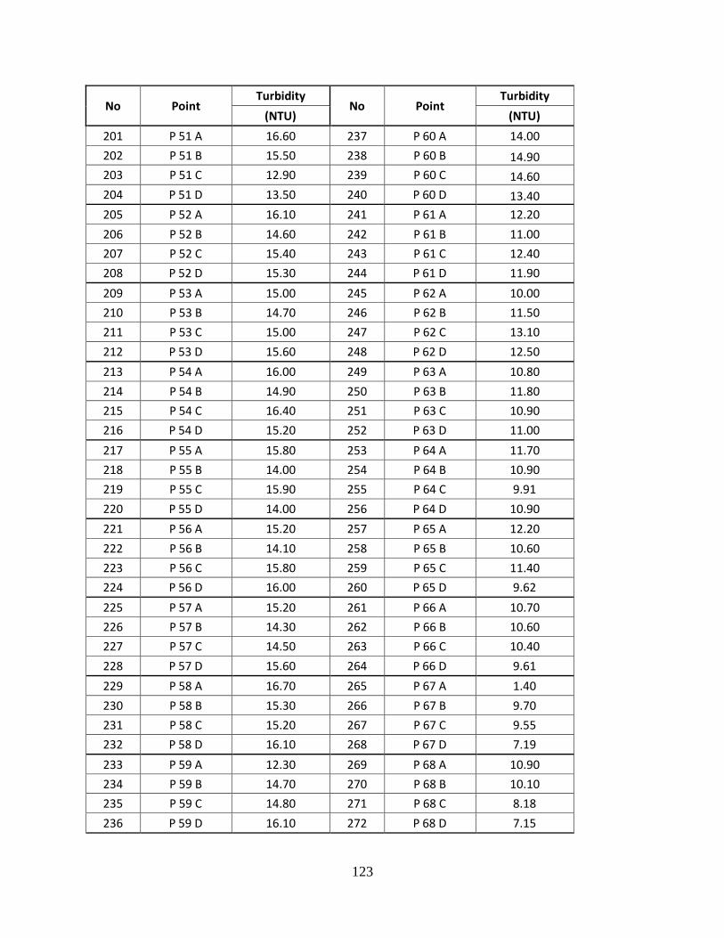
123
No Point Turbidity
No Point Turbidity
(NTU) (NTU)
201 P 51 A 16.60 237 P 60 A 14.00
202 P 51 B 15.50 238 P 60 B 14.90
203 P 51 C 12.90 239 P 60 C 14.60
204 P 51 D 13.50 240 P 60 D 13.40
205 P 52 A 16.10 241 P 61 A 12.20
206 P 52 B 14.60 242 P 61 B 11.00
207 P 52 C 15.40 243 P 61 C 12.40
208 P 52 D 15.30 244 P 61 D 11.90
209 P 53 A 15.00 245 P 62 A 10.00
210 P 53 B 14.70 246 P 62 B 11.50
211 P 53 C 15.00 247 P 62 C 13.10
212 P 53 D 15.60 248 P 62 D 12.50
213 P 54 A 16.00 249 P 63 A 10.80
214 P 54 B 14.90 250 P 63 B 11.80
215 P 54 C 16.40 251 P 63 C 10.90
216 P 54 D 15.20 252 P 63 D 11.00
217 P 55 A 15.80 253 P 64 A 11.70
218 P 55 B 14.00 254 P 64 B 10.90
219 P 55 C 15.90 255 P 64 C 9.91
220 P 55 D 14.00 256 P 64 D 10.90
221 P 56 A 15.20 257 P 65 A 12.20
222 P 56 B 14.10 258 P 65 B 10.60
223 P 56 C 15.80 259 P 65 C 11.40
224 P 56 D 16.00 260 P 65 D 9.62
225 P 57 A 15.20 261 P 66 A 10.70
226 P 57 B 14.30 262 P 66 B 10.60
227 P 57 C 14.50 263 P 66 C 10.40
228 P 57 D 15.60 264 P 66 D 9.61
229 P 58 A 16.70 265 P 67 A 1.40
230 P 58 B 15.30 266 P 67 B 9.70
231 P 58 C 15.20 267 P 67 C 9.55
232 P 58 D 16.10 268 P 67 D 7.19
233 P 59 A 12.30 269 P 68 A 10.90
234 P 59 B 14.70 270 P 68 B 10.10
235 P 59 C 14.80 271 P 68 C 8.18
236 P 59 D 16.10 272 P 68 D 7.15

124
No Point Turbidity
No Point Turbidity
(NTU) (NTU)
273 P 69 A 11.10 309 P 78 A 11.60
274 P 69 B 11.90 310 P 78 B 8.75
275 P 69 C 11.60 311 P 78 C 9.05
276 P 69 D 9.81 312 P 78 D 10.40
277 P 70 A 8.37 313 P 79 A 11.70
278 P 70 B 7.06 314 P 79 B 9.37
279 P 70 C 10.00 315 P 79 C 10.20
280 P 70 D 10.30 316 P 79 D 10.20
281 P 71 A 10.20 317 P 80 A 15.40
282 P 71 B 8.60 318 P 80 B 10.00
283 P 71 C 10.20 319 P 80 C 8.60
284 P 71 D 13.40 320 P 80 D 10.50
285 P 72 A 10.20 321 P 81 A 15.00
286 P 72 B 9.99 322 P 81 B 10.60
287 P 72 C 11.00 323 P 81 C 10.90
288 P 72 D 9.68 324 P 81 D 10.90
289 P 73 A 11.20 325 P 82 A 8.68
290 P 73 B 10.60 326 P 82 B 12.50
291 P 73 C 10.20 327 P 82 C 10.50
292 P 73 D 10.10 328 P 82 D 10.90
293 P 74 A 13.00 329 P 83 A 13.70
294 P 74 B 10.20 330 P 83 B 10.50
295 P 74 C 9.46 331 P 83 C 9.20
296 P 74 D 13.00 332 P 83 D 18.90
297 P 75 A 10.40 333 P 84 A 16.10
298 P 75 B 10.30 334 P 84 B 12.40
299 P 75 C 9.73 335 P 84 C 9.53
300 P 75 D 10.30 336 P 84 D 14.00
301 P 76 A 11.40 337 P 85 A 15.20
302 P 76 B 10.80 338 P 85 B 8.78
303 P 76 C 9.99 339 P 85 C 11.70
304 P 76 D 10.10 340 P 85 D 13.90
305 P 77 A 11.60 341 P 86 A 15.60
306 P 77 B 10.10 342 P 86 B 10.50
307 P 77 C 10.20 343 P 86 C 11.40
308 P 77 D 10.50 344 P 86 D 13.60

125
No Point Turbidity
No Point Turbidity
(NTU) (NTU)
345 P 87 A 20.40 381 P 95 A 14.60
346 P 87 B 9.47 382 P 95 B 11.20
347 P 87 C 10.90 383 P 95 C 10.60
348 P 87 D 16.20 384 P 95 D 9.31
349 P 88 A 23.90 385 P 96 A 11.20
350 P 88 B 11.00 386 P 96 B 10.20
351 P 88 C 10.70 387 P 96 C 11.40
352 P 88 D 18.10 388 P 96 D 13.00
353 P 89 A 16.40 389 P 97 A 16.20
354 P 89 B 10.70 390 P 97 B 11.50
355 P 89 C 15.70 391 P 97 C 14.90
356 P 89 D 15.90 392 P 97 D 14.70
357 P 90 A 20.10 393 P 98 A 15.70
358 P 90 B 11.40 394 P 98 B 14.00
359 P 90 C 5.86 395 P 98 C 11.40
360 P 90 D 13.70 396 P 98 D 14.40
361 P 90 A 12.30 397 P 99 A 11.10
362 P 90 B 11.60 398 P 99 B 11.00
363 P 90 C 6.14 399 P 99 C 11.60
364 P 90 D 13.50 400 P 99 D 11.80
365 P 91 A 12.70 401 P 100 A 15.50
366 P 91 B 20.80 402 P 100 B 13.00
367 P 91 C 11.40 403 P 100 C 10.40
368 P 91 D 13.30 404 P 100 D 13.20
369 P 92 A 13.40 405 P 101 A 13.70
370 P 92 B 12.60 406 P 101 B 11.70
371 P 92 C 14.00 407 P 101 C 14.40
372 P 92 D 14.80 408 P 101 D 19.80
373 P 93 A 13.90 409 P 102 A 18.20
374 P 93 B 10.40 410 P 102 B 17.40
375 P 93 C 11.50 411 P 102 C 11.90
376 P 93 D 13.30 412 P 102 D 16.30
377 P 94 A 14.10 413 P 103 A 17.10
378 P 94 B 9.61 414 P 103 B 11.10
379 P 94 C 12.40 415 P 103 C 16.00
380 P 94 D 14.40 416 P 103 D 17.10
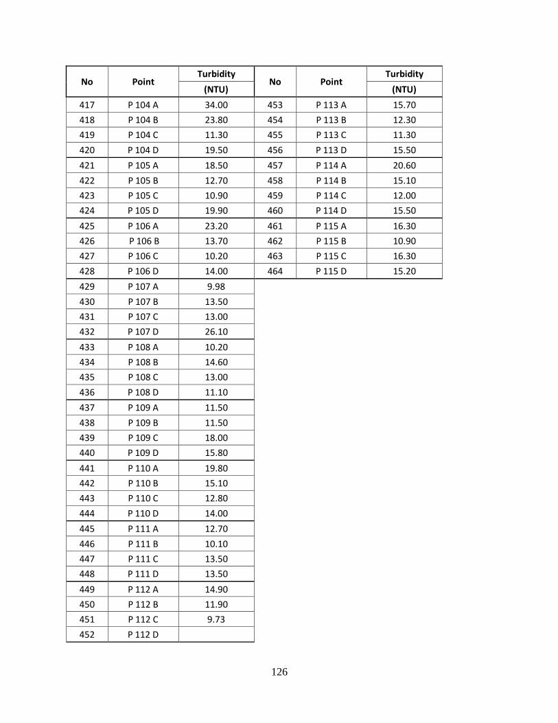
126
No Point Turbidity
No Point Turbidity
(NTU) (NTU)
417 P 104 A 34.00 453 P 113 A 15.70
418 P 104 B 23.80 454 P 113 B 12.30
419 P 104 C 11.30 455 P 113 C 11.30
420 P 104 D 19.50 456 P 113 D 15.50
421 P 105 A 18.50 457 P 114 A 20.60
422 P 105 B 12.70 458 P 114 B 15.10
423 P 105 C 10.90 459 P 114 C 12.00
424 P 105 D 19.90 460 P 114 D 15.50
425 P 106 A 23.20 461 P 115 A 16.30
426 P 106 B 13.70 462 P 115 B 10.90
427 P 106 C 10.20 463 P 115 C 16.30
428 P 106 D 14.00 464 P 115 D 15.20
429 P 107 A 9.98
430 P 107 B 13.50
431 P 107 C 13.00
432 P 107 D 26.10
433 P 108 A 10.20
434 P 108 B 14.60
435 P 108 C 13.00
436 P 108 D 11.10
437 P 109 A 11.50
438 P 109 B 11.50
439 P 109 C 18.00
440 P 109 D 15.80
441 P 110 A 19.80
442 P 110 B 15.10
443 P 110 C 12.80
444 P 110 D 14.00
445 P 111 A 12.70
446 P 111 B 10.10
447 P 111 C 13.50
448 P 111 D 13.50
449 P 112 A 14.90
450 P 112 B 11.90
451 P 112 C 9.73
452 P 112 D
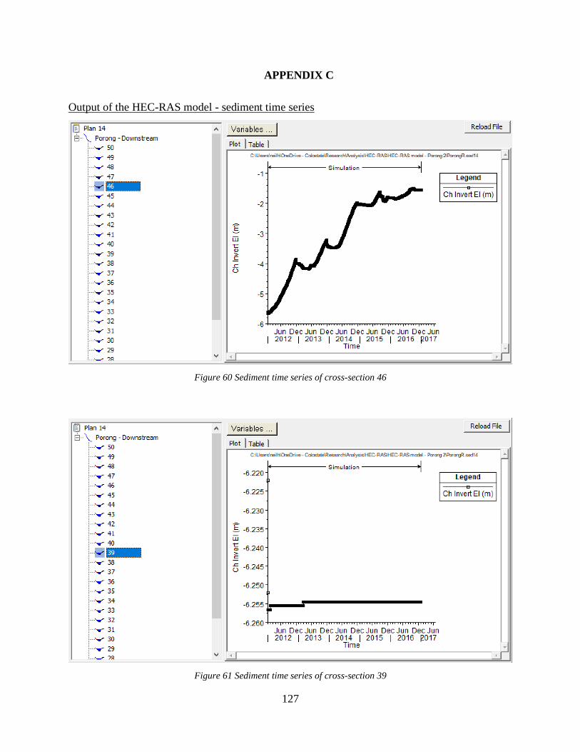
127
APPENDIX C
Output of the HEC-RAS model - sediment time series
Figure 60 Sediment time series of cross-section 46
Figure 61 Sediment time series of cross-section 39
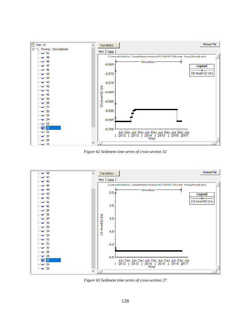
128
Figure 62 Sediment time series of cross-section 32
Figure 63 Sediment time series of cross-section 27