dissertation docteur de lÕuniversit du...
TRANSCRIPT

PhD-FSTC-2016-16 The Faculty of Sciences, Technology and Communication
DISSERTATION
Defense held on 30/05/2016 in Luxembourg
to obtain the degree of
DOCTEUR DE L’UNIVERSITÉ DU LUXEMBOURG
EN INFORMATIQUE
by
Dimitrios KAMPAS Born on 23rd February 1981 in Heraklion (Greece)
TOPIC IDENTIFICATION CONSIDERING WORD ORDER
BY USING MARKOV CHAINS
Dissertation Defense Committee Dr Christoph SCHOMMER, Supervisor Associate Professor, University of Luxembourg Dr. Pascal BOUVRY, Deputy Chairman Professor, University of Luxembourg Dr .Ulrich SORGER, Chairman Professor, University of Luxembourg Dr. Philipp TRELEAVEN, Member Professor, University College London, United Kingdom Dr. Jürgen ROLSHOVEN, Member Professor, University of Cologne, Germany

Preface
The research provided hereunder was conducted between June 2012 and May 2016
under the supervision of Professor Christoph Schommer. Following the list of publi-
cations is exposed.
• Dimitrios Kampas, Christoph Schommer, and Ulrich Sorger. A Hidden Markov
Model to detect relevance in financial documents based on on/off topics. Eu-
ropean Conference on Data Analysis, 2014.
• Dimitrios Kampas and Christoph Schommer. A Hybrid Classification System
to Find Financial News that are Relevant. European Conference on Data Anal-
ysis, 2013.
• Roxana Bersan, Dimitrios Kampas, and Christoph Schommer. A Prospect on
How to Find the Polarity of Financial News by Keeping an Objective Stand-
point. International Conference on Agents and Artificial Intelligence, 2012.
2

Acknowledgements
My greatest thanks to my principal advisor professor Christoph Schommer who has
been an excellent mentor for my thesis. Professor Schommer provided me with
great feedback in the tough moments and assisted me to clarify my research goals.
Our frequent discussions were fruitful and helped me to shape my professional and
research thinking. Moreover, he was always available to listen the issues emerged
and provide his valuable help and support.
I would like to thank professor Ulrich Sorger for his simplicity and elegance. Our
long discussions assisted me to get a better insight of topic models and inspirited
my work. Professor Sorger provided me with great comments and suggestions and
his assistance on the technical parts of my work was important. A special thank to
professor Pascal Bouvry for his support and his insightful comments and suggestions.
I am fortunate to have interacted with a couple of superb colleagues who con-
tributed to my work. A great thank to Mihail Minev for his assistance and scientific
advises and Sviatlana Danilava for her meticulous scientific suggestions.
Writing acknowledgment without mentioning my friends is unthinkable. I would
like to thank Vincenzo Lagani for the time he took to provide me with his scientific
experience and his positive outlook. I would like to thank my friend Panos Tsaknias
who provided me with generous support and honest advises. I would to express my
gratitude to my friend and neighbor Assaad Moawad for his generous help and all
the human values I found in him. I am deeply indebted and thankful to my friends
Rena, Dimitris and Evi for their encouragement, love and mental support during the
difficult times.
I would like to express my heartfelt thanks to my parents since they always stand
3

next to me without negotiating their love. They support me spiritually on writing
this thesis and in my life in general. I would like to express my biggest gratitude
to my brother, who is my friend and my family. I would like to thank him for all
the warm encouragement and deep appreciation on me. Last but not least, I would
like to thank my girlfriend Nancy for the companionship and support in writing this
thesis as well as her efforts to make the daily things of my life easier. I also appreciate
the time she took to improve some of my English.
This small piece of work is dedicated to my nephews Yannis and Michel hoping
that one day I will have the chance to read their PhD thesis.
4

Abstract
Automated topic identification of text has gained a significant attention since a vast
amount of documents in digital forms are widespread and continuously increasing.
Probabilistic topic models are a family of statistical methods that unveil the latent
structure of the documents defining the model that generates the text a priori.
They infer about the topic(s) of a document considering the bag-of-words assump-
tion, which is unrealistic considering the sophisticated structure of the language. The
result of such a simplification is the extraction of topics that are vague in terms of
their interpretability since they disregard any relations among the words that may
settle word ambiguity. Topic models miss significant structural information inherent
in the word order of a document.
In this thesis, we introduce a novel stochastic topic identifier for text data that ad-
dresses the above shortcomings. The primary motivation of this work is initiated
by the assertion that word order reveals text semantics in a human-like way. Our
approach recognizes an on-topic document trained solely on the experience of an
on-class corpus. It incorporates the word order in terms of word groups to deal with
data sparsity of conventional n-gram language models that usually require a large
volume of training data. Markov chains hereby provide a reliable potential to cap-
ture short and long range language dependencies for topic identification. Words are
deterministically associated with classes to improve the probability estimates of the
infrequent ones. We demonstrate our approach and motivate its eligibility on several
datasets of different domains and languages. Moreover, we present a pioneering work
by introducing a hypothesis testing experiment that strengthens the claim that word
order is a significant factor for topic identification. Stochastic topic identifiers are
a promising initiative for building more sophisticated topic identification systems in
the future.

Contents
1 Introduction 1
1.1 Study Motivation . . . . . . . . . . . . . . . . . . . . . . . . . . . . . 1
1.2 Natural Language and Topic . . . . . . . . . . . . . . . . . . . . . . . 5
1.3 Objectives . . . . . . . . . . . . . . . . . . . . . . . . . . . . . . . . . 7
1.4 Thesis Outline . . . . . . . . . . . . . . . . . . . . . . . . . . . . . . . 8
2 Related Works 11
2.1 Probabilistic Topic Models . . . . . . . . . . . . . . . . . . . . . . . . 12
2.1.1 Mixture of Unigrams . . . . . . . . . . . . . . . . . . . . . . . 14
2.1.2 Probabilistic Latent Semantic Indexing . . . . . . . . . . . . . 16
2.1.3 Latent Dirichlet Allocation . . . . . . . . . . . . . . . . . . . . 19
2.1.4 Latent Dirichlet Allocation Extensions . . . . . . . . . . . . . 21
2.2 Text Classification . . . . . . . . . . . . . . . . . . . . . . . . . . . . 24
2.2.1 Naıve Bayes . . . . . . . . . . . . . . . . . . . . . . . . . . . . 25
2.2.2 Support Vector Machines . . . . . . . . . . . . . . . . . . . . . 26
2.3 Discussion . . . . . . . . . . . . . . . . . . . . . . . . . . . . . . . . . 29
3 MTI Methodology 32
3.1 Introduction . . . . . . . . . . . . . . . . . . . . . . . . . . . . . . . . 32
3.2 Milestones . . . . . . . . . . . . . . . . . . . . . . . . . . . . . . . . . 35
3.3 Notation . . . . . . . . . . . . . . . . . . . . . . . . . . . . . . . . . . 36
3.4 MTI Definition . . . . . . . . . . . . . . . . . . . . . . . . . . . . . . 37
3.5 Word Groups Constitution . . . . . . . . . . . . . . . . . . . . . . . . 42
ii

3.5.1 Manually Crafted Word Groups . . . . . . . . . . . . . . . . . 42
3.5.2 Weighting Schemes Crafted Word Groups . . . . . . . . . . . 45
3.6 MTI Training . . . . . . . . . . . . . . . . . . . . . . . . . . . . . . . 48
3.6.1 Document Representation and Pre-processing . . . . . . . . . 48
3.6.2 Inference and Learning . . . . . . . . . . . . . . . . . . . . . . 49
3.6.3 Document Classification . . . . . . . . . . . . . . . . . . . . . 51
3.6.4 Classification Boundary Identification . . . . . . . . . . . . . . 53
4 MTI Evaluation 55
4.1 Data Acquisition . . . . . . . . . . . . . . . . . . . . . . . . . . . . . 55
4.1.1 Federal Reserve Datasets . . . . . . . . . . . . . . . . . . . . . 55
4.1.2 American National Corpus . . . . . . . . . . . . . . . . . . . . 57
4.1.3 HC German Corpora . . . . . . . . . . . . . . . . . . . . . . . 58
4.1.4 Corpora Overview . . . . . . . . . . . . . . . . . . . . . . . . 60
4.2 Validation Techniques . . . . . . . . . . . . . . . . . . . . . . . . . . 60
4.3 Evaluation Measures . . . . . . . . . . . . . . . . . . . . . . . . . . . 65
4.4 Results . . . . . . . . . . . . . . . . . . . . . . . . . . . . . . . . . . . 69
4.4.1 Evaluation Classifiers Selection . . . . . . . . . . . . . . . . . 70
4.4.2 Experimental Scenario I . . . . . . . . . . . . . . . . . . . . . 71
4.4.3 Experimental Scenario II . . . . . . . . . . . . . . . . . . . . . 73
4.4.4 Experimental scenario III . . . . . . . . . . . . . . . . . . . . 75
4.4.5 Word Order Impact on Topic Recognition . . . . . . . . . . . 77
5 Summary 84
5.1 Conclusions . . . . . . . . . . . . . . . . . . . . . . . . . . . . . . . . 84
5.2 Shortcomings and Future Work . . . . . . . . . . . . . . . . . . . . . 87
Appendices 90
A Stopwords Model . . . . . . . . . . . . . . . . . . . . . . . . . . . . . 91
B TF IDF Model . . . . . . . . . . . . . . . . . . . . . . . . . . . . . . 95
C LDA3 Model . . . . . . . . . . . . . . . . . . . . . . . . . . . . . . . 99
iii

Bibliography 100
iv

List of Figures
1.1 Each Latent Dirichlet Allocation (LDA) topic (column) lists sixteen
words. Next to each word is assigned the probability of the term to
belong to the corresponding LDA topic (L-topic) [54]. . . . . . . . . . 2
2.1 The generative process of topic models with two topics and three doc-
uments [54]. . . . . . . . . . . . . . . . . . . . . . . . . . . . . . . . . 13
2.2 The mixture of unigrams model . . . . . . . . . . . . . . . . . . . . . 15
2.3 The probabilistic latent semantic indexing model . . . . . . . . . . . 17
2.4 The latent Dirichlet allocation topic model . . . . . . . . . . . . . . . 21
2.5 The generating phase of composite model [26] . . . . . . . . . . . . . 23
2.6 Support vector machine hyperplane . . . . . . . . . . . . . . . . . . . 27
2.7 Soft margin support vector machines . . . . . . . . . . . . . . . . . . 28
3.1 Finite state machine with three possible states . . . . . . . . . . . . . 38
3.2 State diagram of Stopwords Model . . . . . . . . . . . . . . . . . . . 44
3.3 Boundary variation on different ν values . . . . . . . . . . . . . . . . 54
4.1 Holdout validation method . . . . . . . . . . . . . . . . . . . . . . . 61
4.2 Learning curve of different learners on text data [2]. It demonstrates
the rising accuracy performance as the training set is increasing. . . . 62
4.3 Cross-validation method with five folds. Each iteration uses the one
fifth of the data for testing. The five folds are equally sized and disjoint. 63
4.4 Stopwords Model scores histograms and densities . . . . . . . . . . . 79
4.5 TF IDF Model scores histograms and densities . . . . . . . . . . . . . 80
v

4.6 Beige Book permutations distribution . . . . . . . . . . . . . . . . . . 81
4.7 MASC permutations distribution . . . . . . . . . . . . . . . . . . . . 82
vi

List of Tables
3.1 Notation . . . . . . . . . . . . . . . . . . . . . . . . . . . . . . . . . . 36
3.2 Proposed approach notation . . . . . . . . . . . . . . . . . . . . . . . 40
4.1 MASC topics specification . . . . . . . . . . . . . . . . . . . . . . . . 57
4.2 HC topics-documents specification . . . . . . . . . . . . . . . . . . . . 58
4.3 HC corpus sources . . . . . . . . . . . . . . . . . . . . . . . . . . . . 59
4.4 Corpora specification . . . . . . . . . . . . . . . . . . . . . . . . . . . 60
4.5 Confusion matrix . . . . . . . . . . . . . . . . . . . . . . . . . . . . . 65
4.6 Terminology of confusion matrix . . . . . . . . . . . . . . . . . . . . . 66
4.7 Classification performance measures . . . . . . . . . . . . . . . . . . . 68
4.8 Classification results - Experimental scenario I . . . . . . . . . . . . . 72
4.9 Classification results - Experimental scenario II . . . . . . . . . . . . 74
4.10 Experimental Scenario III - Health vs Crime & Law . . . . . . . . . . 75
4.11 Experimental Scenario III - Health vs Travel . . . . . . . . . . . . . . 76
4.12 Corpora standard deviation . . . . . . . . . . . . . . . . . . . . . . . 78
4.13 Permutation correlations . . . . . . . . . . . . . . . . . . . . . . . . . 83
A.1 Stopwords Model ten-fold cross validation performance on FOMC -
MASC corpora . . . . . . . . . . . . . . . . . . . . . . . . . . . . . . 91
A.2 Stopwords Model ten-fold cross validation performance on FOMC -
Beige Book corpora . . . . . . . . . . . . . . . . . . . . . . . . . . . 92
A.3 Stopwords Model ten-fold cross validation performance on HC Health
- HC Crime & Law corpora . . . . . . . . . . . . . . . . . . . . . . . 93
vii

A.4 Stopwords Model ten-fold cross validation performance on HC Health
- HC Travel corpora . . . . . . . . . . . . . . . . . . . . . . . . . . . 94
B.1 TF IDF Model ten-fold cross validation performance on FOMC - MASC
corpora . . . . . . . . . . . . . . . . . . . . . . . . . . . . . . . . . . 95
B.2 TF IDF Model ten-fold cross validation performance on FOMC - Beige
Book corpora . . . . . . . . . . . . . . . . . . . . . . . . . . . . . . . 96
B.3 TF IDF Model ten-fold cross validation performance on HC Health -
HC Crime & Law corpora . . . . . . . . . . . . . . . . . . . . . . . . 97
B.4 TF IDF Model ten-fold cross validation performance on HC Health -
HC Travel corpora . . . . . . . . . . . . . . . . . . . . . . . . . . . . 98
C.1 LDA3 Model ten-fold cross validation performance on FOMC - MASC
corpora . . . . . . . . . . . . . . . . . . . . . . . . . . . . . . . . . . 99
C.2 LDA5 Model ten-fold cross validation performance on FOMC - Beige
Book corpora . . . . . . . . . . . . . . . . . . . . . . . . . . . . . . . 100
viii

List of Acronyms
LDA Latent Dirichlet Allocation
pLSI Probabilistic Latent Semantic Indexing
L-topic LDA topic
LSI Latent Semantic Indexing
IR Information Retrieval
MLE Maximum Likelihood Estimation
CTM Correlated Topic Model
HMM Hidden Markov Model
IDF Inverse Document Frequency
SVD Singular Value Decomposition
TF Term Frequency
NLP Natural Language Processing
BoW bag-of-words
NB Naıve Bayes
CRP Chinese Restaurant Process
HMM Hidden Markov Model
STM Syntactic Topic Model
SVM Support Vector Machines
NLP Natural Language Processing
ix

FED Federal Reserve Bank
FOMC Federal Reserve Open Market Committee
OANC Open American National Corpus
MASC Manually Annotated Sub-Corpus
MTI Markovian Topic Identifiers
MLE Maximum Likelihood Estimation
LTS Logarithmic Topic Score
MCC Matthews Correlation Coefficient
x
Chapter 1
Introduction
1.1 Study Motivation
The amount of documents available in digital form is overwhelming and continuously
increasing. Nowadays there is a growing interest in digesting the information pro-
vided in the text. Considering the limitations of human processing capacity, more
automatic text processing approaches have been developed to address the issue of
text understanding. When dealing with a big collection of text documents, it would
be convenient for each document to have a“short description” that could briefly give
us what it is about. We may use it to select the text(s) of interest or achieve a text
overview. Moreover, we may use the extracted information to introduce new metrics
to categorize, cluster or measure the “similarity” or “relevance” of documents.
Numerous approaches have been developed on how to extract content-features based
on different statistical weights [42, 50]. Recently, probabilistic topic models have
gained significant attention as a modern way to capture semantic properties of doc-
uments. LDA [9] which is a widely used topic identification method on large corpora
considers that documents are mixtures of distributions over words. LDA outputs
sets-of-words out of a collection of documents naming each individual set, a topic1 as
1We call the topic of LDA as L-topic to distinguish by the human perception of topic
1

it is demonstrated in Figure 1.1. They claim [9] that the significantly co-occurring
words in a document provide us with the LDA topics (L-topics) of a document.
For instance, they expect the terms “pasta” and “pizza” to appear in a document
discussing about Italian food. They employ the extracted sets-of-words to assign
L-topic mixtures to documents regarding their word proportion or they classify texts
regarding their L-topic similarity (word proportion).
Figure 1.1: Each LDA topic (column) lists sixteen words. Next to each word isassigned the probability of the term to belong to the corresponding L-topic [54].
To infer about the document L-topics, LDA relies on the following assumptions:
• Documents are generated by initially choosing a document-specific distribution
over L-topics, and then repeatedly selecting an L-topic from this distribution
and drawing a word from the L-topic selected.
• The permutation of the words in the document let the model unaffected - each
document is modeled as a bag-of-words (BoW).
The latter assumption implies that the document structure is disregarded. The key
insight of LDA is the premise that words convey strong semantic information about
2

the content of the document. In other words, Blei et al. assume that texts on simi-
lar L-topics consist of the similar BoW. LDA definition of topic neglects other text
semantics; the authors mention [9] that: “A topic is characterized by a distribution
over the words in the vocabulary” and “the word distributions can be viewed as repre-
sentations of topics”. But, the fact that the word order is ignored is the main deficit
of this method; in fact, it is an important component [1] of the document structure
since two passages may have the same words statistics, nonetheless, different topics.
For example, the passages “the department chair couches offers” [56] and “the chair
department offers couches” [56] convey different topics but the vocabularies and the
word frequencies are identical.
The above example depicts that the human perception of topic encompasses the word
order. After LDA was published several works remark and deal with word order as a
significant factor to improve the quality of topics [58, 53, 41] and the performance of
clustering or classification systems. Word order has been considered as an indicative
factor for topic inference and a fundamental element to improve natural language
representation. In 2006 Wallach [56] claimed that: “It is likely that word order can
assist in topic inference”. In 2013, Shoaib et al. [53] claimed that: “Some recent topic
models have demonstrated better qualitative and quantitative performance when the
bag-of-words assumption is relaxed”, thus they introduced a model that is no longer
invariant to word reshuffling since it preserves the ordering of the words [53]. In 2009,
Andrews et al. [1] discuss the importance of word order in semantic representation.
They claim that: “The sequential order in which words occur (...) provide vital
information about the possible meaning of words. This information is unavailable
in bag-of-words models and consequently the extent to which they can extract seman-
tic information from text, or adequately model human semantic learning, is limited.”.
In this thesis, we study the word impact on topic recognition by introducing a model
to improve topic inference incorporating the order of words. Our topic identification
approach considers the sequential statistics of documents. It extends the prevalent
bag-of-words paradigm and infers about the topic discourse of text by considering
3

the inherent sequential semantics. The goal of our model is to classify a document
as ‘on’ - close with a domain specific discourse - or ‘off’ otherwise. It detects similar
structural properties of a new document with respect to the provided input.
However, it is not a conventional binary classifier since it relies exclusively on the
experience of documents of one class. We often need to recognize documents of a
particular topic out of an ocean of ‘off’ documents because it is easy to gather data
on the requested situation and it is rather expensive or impossible to do the same
for data of undesirable situations. In this setup, ordinary classification systems are
inappropriate since they require training in the entire universe of topics to be effec-
tive.
A promising approach to incorporate word sequence applied on different applications
related to natural language is using a Markovian model. In literature, Markovian
models have been used on text to perform topic segmentation [8, 45, 53], LDA-like
topic identification [1, 28, 45] and speech recognition [37, 48]. They provide a way
to model the sequential semantics of the natural language. In this work, we have
modeled a stochastic process for word sequences, where each word is conditionally
dependent of its preceding words. A Markov chain hereby provide a reliable potential
to incorporate language and domain dependencies for topic recognition. They are
trained to employ knowledge provided about the corpus words and recognize topics
regarding the sequential statistics of the input. The knowledge used is tuned and
gauged to achieve superior results.
4

1.2 Natural Language and Topic
The problem for scientists that deal with natural language is that human language
holds ambiguities. First, different words may convey the same meaning and each
word might have diverse meanings in different sentences. Second, at the sentence
level, the valid sequence of parts of speech, might have more than one reasonable
structure making it challenging to disambiguate the sentence meaning. Although
humans deal with natural language ambiguities effectively, it is not straightforward
how machines can deal with them.
The complexity of human language makes abstract notions like meaning or topic
difficult to be addressed. In topic research a central question someone may meet is:
What is a topic? Provided an answer to this question might reflect the building of
systems that perform effectively on identifying topics.
Linguists provide many definitions of a topic. In 1983, Brown and Yule [23] stated
that “the notion of topic is clearly an intuitively satisfactory way of describing the
unifying principle which makes one stretch of discourse ‘about’ something and the
next stretch ‘about’ something else, for it is appealed to very frequently in the dis-
course analysis literature”. According to the authors, the topic is a very frequent
- but usually undefined - term in discourse analysis. It has been used to represent
various meanings; Hockett [32] in 1958 used the term as a grammatical constituent
to describe sentence structure. In 1976 Keenan and Schieffelin [39] introduced the
term discourse topic that it was further explained by Brown and Yule in 1983 as the
notion of “what is being talked/written about”.
In computer science literature a topic is defined as a distribution over the vocabulary
[9]. Blei et al. [9] state that: “We refer to the latent multinomial variables in the
LDA model as topics, so as to exploit text-oriented intuitions, but we make no episte-
mological claims regarding these latent variables beyond their utility in representing
probability distributions on sets of words.” The previous quote implies that there
5

was not much research on further notions of topic. Actually, for computer scientists
topics are set of words that are used as features to accomplish other tasks such as
document similarity.
Apparently, the definition of topic in topic modeling disregards any information
about the topic structure. On the contrary, linguistic definitions of topic [23, 32, 39]
are rather abstract to be utilized by machines for topic identification. Although,
humans can recognize the topic of their interest in a straightforward manner, it is
challenging for scientists to pin down the procedure of automatic topic recognition.
It is challenging for human to provide the characteristics of the topic since it is a
multidimensional problem associated with the human intuition and personal inter-
pretation [14, 31].
This thesis does not address the problem of what a topic is. Instead, we scrutinize
a division of how to identify a topic in a piece of text. Therefore, we assume that
regardless of what a topic may be, it remains latent but somehow common knowl-
edge. We define a topic as the stochastic model that best recognizes what humans
consider as topics, modeling human semantic learning. We consider words and the
word sequence as the language aspects to be indicative of the latent topic. In this
thesis, we ignore any fine-granular distinctions between topic, field, theme et cetera.
We considered a particular probabilistic model, which we train to develop a robust
topic model oriented to formal written language. We aim to distinguish documents
of subtly different topics in terms of akin vocabularies experimenting on financial re-
ports. We examine the possibilities to generalize by introducing various probabilistic
topic models that we apply on the same datasets.
6

1.3 Objectives
The task of topics identification on written documents is a manifold assignment. Not
only due to the fact that a clear definition of what a topic is or how a topic look like is
missing (Subsection 1.2), but also because of the complexity and ambiguity of natu-
ral language texts. Natural language complexity makes inference assumption of topic
identification or classification methods to look as oversimplifications. Therefore, the
outcome of such methods is inaccurate considering the human understanding of topic.
In computer science, the task of topic identification has been considered as an in-
termediate step to perform several other tasks on large collections of documents like
organization, summarization, large corpora exploration et cetera. As far as the final
task provides a satisfactory outcome no further investigations have been conducted
on how to actually improve topic identification. A reason for that might be what Blei
claims in a review of 2011 [4] : “There is a disconnect between how topic models are
evaluated and why we expect topic models to be useful”. Moreover, questions related
to topic evaluation and topic model assumptions “have been scrutinized less for the
scale of problems that machine learning tackles” [4]. In other words, the assumptions
of topic models and their outcome are not subject of scrutinized research.
In this thesis, we extend the prevalent bag-of-words assumption exploring the perfor-
mance of topic identifier that encompass the word sequence of text. Consequently,
the research question is:
1. How well a stochastic topic identifier can perform on discriminating text of
different domains and languages?
The bag-of-words representation facilitates the inference of complex statistical mod-
els due to the simplification of the representation. The scenario in which the word
order is considered in a conventional topic model, would lead to intractable calcula-
tions. In this work, we keep the complexity of the model moderate to facilitate the
study of this research question.
7

Secondary, current topic models incorporate no prior knowledge about the ‘semantics’
of natural language. They are applied to a collection of not annotated documents
with no other information provided because their primary goal is to give an insight of
the corpus. In this work, we encompass prior knowledge in terms of sets of words with
common characteristics. In this way, we indent to enhance model’s discriminating
performance.
2. What form of prior knowledge would increase the topic identification efficiency
of the introduced model?
Many different pieces of knowledge can be incorporated regarding different criteria.
In our case, we heuristically explore the role of different linguistic components i.e
stopwords to boost the detection efficacy of the model.
Finally, several works [58, 53, 41] highlight the importance of word order as a signifi-
cant factor to perform topic inference and a key element to improve natural language
representation. Thus, they explore the efficacy of unsupervised and supervised meth-
ods that consider word order in their premise. Nevertheless, a quantification analysis
that exhibits the importance of word order in the text is missing. The third research
question is the following:
3. Which is the impact of word order, as an additional property of bag-of-words,
on topic identification?
To answer the above question we introduce a hypothesis testing experiment that
randomly generates documents out of a particular vocabulary and compares them
with the original documents probing the differences in topics. The next sections
outline the corresponding milestones.
1.4 Thesis Outline
Chapter 1 discusses the background and motivation of the research work of this the-
sis. Moreover, it provides the notion of topic as it is introduced in literature and
8

clarifies the direction of this research work. It specifies the research questions we
deal with in the next chapters.
Chapter 2 is dedicated to provide an overview of the related works. First, it summa-
rizes probabilistic topic models giving the development of them in time until LDA
was introduced. The basic concepts and the modeling fundaments are introduced.
Modern variations and improvements of LDA are provided as well. Some classifica-
tion methods are introduced because to some extent they may be used to discriminate
documents of different topics besides the fact that we use some classification methods
as a comparison to assess the efficacy of our approach. At the end advantages and
disadvantages of the introduced methods are provided and a discussion of what is
missing in the literature is given.
Chapter 3 is dedicated to the introduced approach. The milestones are given and
in the next sections, a set of methods to recognize topics are provided. A set of
stochastic models that consider word order are formalized and the inference and
learning is provided. At the end the classification steps of a new given document are
described and the classification boundary is identified. We name the set of identifiers
we introduced Markov topic identifiers (MTI) since they are based on Markov chains
to incorporate word order.
In Chapter 4 we provide a number of test scenarios on different datasets to evaluate
the Markovian topic identifiers performance. We discuss the presented results com-
pared with the baseline results provided by the widely used classifiers of naıve Bayes
and support vector machines. Different measures are used to assess the models per-
formance in a ten-fold cross validation schema. The implemented experiments reflect
the introduced research question of Section 1.3. The number of classified samples
are provided in the appendix sections where each section is dedicated to a model
introduced. In Chapter 5 we summarize the overall research work and we provide
potentials and shortcomings it exhibits. We suggest extensions and possible appli-
cations of the introduced model as well.
9

10

Chapter 2
Related Works
This chapter is dedicated to present the state-of-the-art of topic identification. We
present works that are related and hold the same objectives like the model proposed
in this thesis. Some of the related work is summarized in the following two Sec-
tions 2.1 and 2.2.
At the beginning, we provide a brief overview of the most important topic models
and their extensions. We present the probabilistic topic models that disregard the
word order in documents, BoW assumption. We highlight the fundamental ideas
behind and the formalization of each single model providing in chronological order
the evolution of topic modeling until latent Dirichlet allocation was introduced. We
later present some extensions of LDA that amend its initial text generation schema
capturing different aspects of a topic like topic evolution or topic correlations corpus-
wide. Moreover, they relax the BoW assumption dealing with word collocations to
form L-topics.
Later, we discuss some of the widely known classifiers that may be used in topic re-
lated tasks to discriminate the topic of a new document. We select the classifications
methods that are representative regarding the inference assumptions and feasible to
be applied on text. For instance back propagation neural networks are not presented
since they exhibit high computational cost to converge on multidimensional problems
11

like topic classification.
Finally, in Section 2.3 we discuss the pros and cons of the probabilistic topic models
and classifiers. We spotlight the improvements we intend to achieve in this thesis
contradicting the already presented methods of this chapter. In particular, we discuss
the advantages of our method in terms of cost-effectiveness and performance that
the two other cannot provide.
2.1 Probabilistic Topic Models
Topic models are a suite of algorithms used to discover the themes of large and un-
structured document collections and can be used to organize the collections. They
are generative statistical models that uncover the hidden thematic structure that has
generated the document collection. They are effective, thus widely used, on applica-
tions in the fields of text classification and Information Retrieval (IR) [4].
In this section, we introduce models where the hidden topic structure of a document
is explicitly provided in the definition of the model. The set of models we discuss
feature a proper hierarchical Bayesian probabilistic framework that permits the use
of wide range of training and inference techniques. The topics of the models are not
a priori determined but rather extracted from the document collection. Once the
training phase is accomplished, the model can infer about new documents using the
statistical inference process. Probabilistic topic models can also be used for vari-
ous tasks like document or topic similarity exploration; they deal with these tasks
by comparing probability distributions over the vocabularies. Thus, methods like
Kullback-Leibler or Jensen-Shannon divergence are applied.
Topic models are considered to be text generators with different statistical assump-
tions about the parameters that generate the text. They infer about the posterior
distribution from the data and they require no prior knowledge or labeling of the
documents. The vocabulary of the documents and the word frequencies is the nec-
12

essary input to the topic models. Moreover, topic models deal effectively with words
of similar meanings and distinguish among words with multiple meanings. They go
one step further annotating documents with thematic information and provide the
relationship among the assigned themes. To achieve their goal they consider that
the words are chosen from sets of polynomial distributions which are used to deduce
about the significantly co-occur words in the collection. They consider that each
document is a mixture of word distributions and they define each individual multi-
nomial distribution to be a topic.
Figure 2.1: The generative process of topic models with two topics and three docu-ments [54].
Figure 2.1 demonstrates a generative process with two topics and three documents.
Topic 1 and topic 2 are about money and river respectively. They exhibit different
word distributions according to the word importance for the topic. Doc1 and Doc3
are produced by topic 1 and topic 2 respectively with weights 1.0, while Doc2 is
generated by an equal mixture of both topics. The superscript on each word indicate
the topic that is employed to draw the word. The way the model is defined does
not presume word exclusivity in topics, i.e., bank occurs in both topics. This allows
topic models to capture word with multiple meanings (polysemy). The generative
13

process described in Figure 2.1 neglects the word order of the documents; this is the
common bag-of-words assumption of many statistical language models.
Following in this section, we will describe the development of probabilistic topic
models from a simple model to recent and sophisticated models that deal with state-
of-the-art issues like the relationship between topics. First, we present the mixture of
unigrams as the primary method to perform topic identification. It is a method close
to Naıve Bayes (NB) which exhibits several deficits. In subsection 2.1.2, we present
Probabilistic Latent Semantic Indexing (pLSI) which is a probabilistic development
of Latent Semantic Indexing (LSI). In 2.1.3 we present the LDA model which is
a development of pLSI. Latent Dirichlet allocation overstepped pLSI shortcomings
assuming that the topics are drawn from a Dirichlet distribution. LDA stimulated
the deployment of several topic models that comprise several extension and amplified
modeling capacities. It goes beyond text analysis and is applied to music and image
analysis. In the following sections, we present significant LDA developments with
diverse setups and various research objectives.
2.1.1 Mixture of Unigrams
In 2000 Nigam et al. introduced a simple generative topic model for documents called
mixture of unigrams. [46]. This model assigns only one topic z for a document and
then a set of N words is generated from the conditional multinomial distribution
p(w|z). This type of model is suitable for supervised classification problems where
the set of possible values of z corresponds to the classification tags. The key idea of
the mixtures of unigrams is that each topic is related to a particular language model
that draw words pertinent to the topic. A mixture of unigrams is identical to naıve
Bayes classifier with Nd the size of the vocabulary and M training documents where
the set of possible topics are given.
The mixture of unigrams model is demonstrated in Figure 2.2. A directed graph
with “plates” is used to represent the model, in which each node indicates a random
variable and the direct edge represents the statistical dependencies between the vari-
14

Figure 2.2: The mixture of unigrams model
ables. The plates express the replication of different parts of the graph. The inner
plate represents the document and the outer plate the collection of documents. The
numbers in the lower-right corners of the plates represent the document collection
size which is M and the document vocabulary which is Nd for a document d. Each
document has a single topic z as is shown in the graph. The graphical model of Fig-
ure 2.2 reveals the conditional probability distributions for the nodes with parents
i.e., w. The conditional probability p(w|d) follows the multinomial distribution. For
the variables without parents a prior distribution is assumed; i.e., for z a multino-
mial distribution over the possible topics is defined. For a document d the following
probability is defined:
p(d) =∑z
p(z)
Nd∏n=1
p(wn|z) (2.1)
Practically, the implementation of the mixture of unigrams model requires the calcu-
lation of the multinomial distributions p(z) and p(w|z). Granted that we are provided
with a set of labeled document, each one annotated with a topic, we can calculate
the parameters of these distributions utilizing the maximum likelihood estimation
(MLE). For this reason, we calculate the frequency of each topic zi that appears in
the collection of documents. We estimate the p(w|z) for each zi by counting the times
each wi appears in all documents assigned with zi. In case that a word wj does not
exist in any documents with label zj; MLE will assign zero probability to p(wj|zj).A number of different smoothing methods (i.e., Laplace[29]) can be applied to ensure
15

that this does not happen. If the topic labels are not provided for the documents
the expectation-maximization technique[19] can be applied. After the training phase
has been completed, the topic inference about new documents can be achieved using
Bayes rule.
2.1.2 Probabilistic Latent Semantic Indexing
One widely studied issue in IR is the query-based document retrieval. Suppose a doc-
ument retrieval system which intends to sort documents regarding their relevance to
a query. The challenge of implementing such a system is to deal with the ambiguity
of natural language and the short length of typical queries that increase the complex-
ity of the system. If we simply build the system on matching words in documents
with words in queries we will end up dropping most relevant documents since short
user queries tend to contain synonyms for the essential words. Another key point is
the polysemy of the words; for instance if a query contains the word ‘bank’ multi-
ple sets of documents will be matched regarding the various meanings of the word.
Documents that discuss the banking sector and rivers will be returned. To address
the previously mentioned issues additional information needs to be considered from
text that reveals the semantic content of a document beyond the set of words itself.
LSI [18, 3] was introduced in 1990 to deal with these concerns in a more effective
manner. LSI is a technique that maps documents in a semantic space with lower
dimensions, for that matter, texts with alike topics will be close each other in the
produced space. The latent topic space in LSI is derived from the word co-occurrence
in the whole collection of documents, on that front, the degree of relevance between
two documents is also a matter of the other documents1 in the collection. The cen-
tral technique that LSI employs comes from linear algebra and it is called Singular
Value Decomposition (SVD) [3]. It is used to perform noise reduction and at the
1Two documents are close whether they share a sufficient big number of words. For example,in the world wide web, two documents that contain words about programming languages will beclose in the latent space. But between two documents in a collection of texts of software engineers,more terms need to be common for the documents to be close.
16

same time, it plummets the scale of the problem.
Nonetheless, The effect of SVD on words has been criticized since it is hard to be
assessed. Therefore, Hofmann introduced probabilistic latent semantic indexing [33]
to provide improvements on LSI. Actually, probabilistic Latent Semantic Indexing
preserves the same objective but it is different from LSI since it has a probabilistic
orientation with a clear theoretical justification that LSI lacks. pLSI is demonstrated
in Figure 2.3 and is described by the following generative model for a document in
a collection:
• Choose a document dm with probability p(d)
• For each word n in dm
– Choose a topic zn from a multinomial conditioned on dm with probability
p(z|dm)
– Choose a word wn from a multinomial conditioned on the previously cho-
sen topic zn with p(w|zn)
Figure 2.3: The probabilistic latent semantic indexing model
From the graphical model of Figure 2.3, we notice that pLSI relies on certain as-
sumptions of independence about the documents in the collections and the words in
the document. More precisely, the words are conditionally dependent of the topics
and conditionally independent of the documents. The key assumption on which pLSI
relies upon is the BoW assumption. In particular, the word order of the document
17

is not incorporated in the model. Additionally, in pLSI model each observed item
(word) of the data is associated with a latent variable (topic); this one-to-one asso-
ciation is called aspect model[34, 51] in literature.
The objective of pLSI is to estimate the probability:
p(w, d) =∑z∈Z
= p(z)P (w|z)p(d|z) (2.2)
Hofmann introduced a version of expectation-maximization to train the model in an
unsupervised manner. In experiments performed by the author, pLSI overstepped
the latent semantic analysis in IR tasks.
pLSI finds various applications in information retrieval and topic classification. In IR
the similarity between query keywords wq and document di needs to be estimated.
This similarity is defined as follows:
Similarity(wq, di) = wq · P (w,w) · dTi (2.3)
where P (w,w) denotes the probability similarity matrix between the words. In topic
classification the key point is to estimate the similarity between two documents di
and dj. wi and wj are the normalized word vectors of the frequencies of the words
that have been calculated from di and dj respectively. The similarity is defined as
follows:
Similarity(di, dj) = di · P (w,w) · dTj (2.4)
Compared to mixture of unigrams, pLSI exhibits enhanced modeling facilities, since
it allows a document to discuss more than one topics. As a matter of fact each
word in a document can be derived from a different topic. Moreover, pLSI has a
broader range of applications than the ad hoc LSI. pLSI relies on a solid theoretical
background that allows it to have a clear interpretation of its results. Nevertheless,
pLSI exhibits a drawback on the assigned topic proportion of a document. By the
generative process of pLSI, we realize that the topic mixture assigned to a document
18

is estimated from the collection. When pLSI deals with standalone IR tasks this
may not be crucial. But, in various other tasks like text categorization, the lack
of flexibility on handling newly seen documents cause issues on document inference.
Coupled with the above, the principle of learning the topic distribution for each
document in the collection leads to a high number of parameters estimations that
grow with the number of documents in the collection making pLSI inappropriate for
large scale datasets.
2.1.3 Latent Dirichlet Allocation
In 2003 Blei et al. published a work named latent Dirichlet allocation [9] which is
one of the most popular topic models. It goes beyond information retrieval and it
is applicable not only to text but on images and music collections. Latent Dirich-
let allocation can be considered as a generalization of pLSI in which the Dirichlet
distribution is utilized to ‘identify’ the topics. On that front, LDA is considered to
be a complete generative probabilistic model with high descriptive power since the
number of model parameters is independent of the number of training documents as
pLSI regards. Additionally, LDA is robust to overfitting thus widely used for large
scale problems.
Let’s suppose that LDA is applied on a corpus of three topics, such as medicine,
finance, and biology. A document that describes a disease treatment may discuss
either medicine and biology topics. The medicine texts have a number of words that
exhibit high probability in appearing in a document related to medicine. Likewise,
there is a set of words that are related to biology with a corresponding probabil-
ity. During the generation process of LDA on a document about disease treatment,
the topics will be randomly selected at the beginning. The probability of selecting
the topics of medicine and biology will be increased and following a word will be
selected. Words that are related to the two topics will have the higher probability
to be selected. After N words have been selected, where N is the vocabulary size
of the document, the selection is accomplished and the document is generated. The
19

formalization of the generative process for a document d is as follows:
• Choose topic proportion θ for document d with a Dirichlet parameter α.
• For each word w ∈ d:
– Choose a topic zn from a multinomial distribution over topics with pa-
rameters θ.
– Choose a word wn from a multinomial distribution over words with pa-
rameters φzn ; where φzn = p(w|zn) is the multinomial conditioned over
words for topic zn.
LDA assumes that a text is constituted of a particular topic multinomial distribution
sampled from a Dirichlet distribution. The number of topics is k and a priori given.
Then, each of these k topics is repeatedly sampled from generate each word in the
document. Therefore, a topic is defined to be a probability distribution of the words.
The documents are described as a mixture of topics with a certain proportion. The
plate graphical representation of LDA is demonstrated in Figure 2.4.
The graphical representation of LDA uses plates to represent the replicates. The
outer plate represents the documents, each one of them is described by a topic mix-
ture θ which is sampled by a Dirichlet distribution with hyperparameter α. The
inner plate represents the repeated sampling from θ. The filled circle represent the
observations (words) and the hollow circles represent the hidden variables of the
model. The arrows represent the dependencies between the linked nodes.
The Dirichlet variables in LDA are vectors θ that receive values in (k − 1) simplex,
thus∑k
i=1 θi = 1. The probability density of a k-dimensional Dirichlet distribution
over the multinomial distribution θ = (θ1, . . . , θk) is defined as:
Dir(a1, . . . , ak) =Γ(∑
i(ai))∏i Γ(aj)
k∏i=1
θai−1i (2.5)
20

Figure 2.4: The latent Dirichlet allocation topic model
where Γ() is the gamma function and the αi are the Dirichlet parameters. Each αi
can be interpreted as a prior observation count on the number of times a topic zn has
appeared in a document, before the training of the model. The implementation of
LDA by the authors uses a single Dirichlet parameter α, such that each αi = α. The
single α parameter results in a smoothed multinomial distribution with parameter θ.
The hyperparameter β is the prior observation count on the number of times words
are sampled from a topic before any observations on the corpus occurred. This is a
smoothing of the word distributions in every topic. In practice, a proper choice of α
and β depends on the number of topics and the vocabulary size.
2.1.4 Latent Dirichlet Allocation Extensions
LDA is a significant topic model on which many researchers based their work to
capture other properties of the text. To do so, they added variables to their models
to describe the development of topics over time, the relationship among topics, the
role of syntax in topic identification and so on. In the following, we briefly present
some of recently introduced topic models where the majority of them are based on
the fundamentals of latent Dirichlet allocation.
In 2006 Blei et al. introduced dynamic topic models [6] to analyze the evolution of
21

topics over time in a sequentially organized corpus of documents. This approach
infers about the latent parameters of the model using the variational method. The
parameters of the model follow the multinomial distribution. A state space repre-
sentation is used to transmit the multinomial parameters upon the words of each
topic. The Correlated Topic Model (CTM) [5] was designed to provide correlation
among topics. The key idea that CTM relies on is that a document discussing about
medicine is more likely to be related to disease than astronomy. The assumption of
LDA that topics are drawn from a Dirichlet distribution confines LDA to provide the
correlation between topics. To facilitate topic correlations, topic models assume that
topics have correlations via the logistic normal distribution that exhibit a sufficient
satisfactory fit on test data.
In 2004 Blei et al. introduced an extension of LDA -named hierarchical latent Dirich-
let allocation [25] - that deals with topics in the manner of hierarchies. On that
front, they combine a nested Chinese Restaurant Process (CRP) with a likelihood
that relies on a hierarchical variant of latent Dirichlet allocation to derive a prior
distribution on hierarchies. In 2010, the supervised topic model [7] was introduced
to deal effectively with prediction problems. They designed a topic model to perform
prediction regarding the vocabulary. They examine the prediction power of words
with respect to the topic class. They compare LDA with supervised topic model and
they find the new model to more effective.
In traditional topic models, such as LDA, most of the syntactic words are removed
since we are only interested in meaning and only long-range dependencies are con-
cerned. Therefore, topic models focus on identifying semantic words through doc-
uments or entire collections. On the contrary, the composite model [26] that was
introduced by Griffiths et al. considers the short-range dependencies as well. It
blends a Hidden Markov Model (HMM) to capture the parts of speech and a latent
Dirichlet allocation to extract words that are deemed semantic. Composite model
competes for part-of-speech taggers and it is not used for topic classification itself.
In Figure 2.5 it is demonstrated the generating phase of this model where an au-
22

tomaton is constructed to describe the structure of the language. Figure 2.5 shows
the transitions of a three class HMM annotated with the corresponding probabilities.
The semantic class shown in the middle consists of three topic sets each one assigned
a probability. The other two classes are simple multinomial distribution over words.
Document phrases are generated by following the transitions of an automaton like
the one in 2.5. Particularly, a word is chosen from the distribution associated with
each syntactic class, a topic follows and a word comes next from a distribution asso-
ciated with that topic for the semantic class.
Figure 2.5: The generating phase of composite model [26]
Although exchangeable word models are useful for classification or information re-
trieval, they are limited for problems that depend on more fine-grained qualities of
language. For instance, a topic model is efficient on providing documents relevant
to queries but it cannot suggest relevant phrases for question answering. Syntactic
Topic Model (STM) [12] is a document model that blends the observed syntactic
structure with the latent thematic structure of a document. STM intends to extract
groups of words that are utilized the same way in similar documents. STM can be
used to incorporate document context into parsing models but is not a full parsing
model. It provides a way to learn both simultaneously rather than combining the
two heterogeneous methods. Syntactic topic models have been used for statistical
natural language generation [17].
23

In 2009, C. Wang et al. introduce a generative probabilistic model [57] to capture
firstly the corpus-wide topic structure and secondly the topic correlation across cor-
pora. They test their model on a dataset extracted from six different computer
science conferences; they evaluate their model on the abstracts parts of the text.
Additionally, researchers have studied the efficiency of topic models on different lev-
els of resolution. Bruber et al. [27] consider that each sentence discusses one topic
and all the words in a sentence are assigned the sentences topic. The goal of the
authors is to perform word sense disambiguation. Wallach [56] extended LDA to fa-
cilitate n-gram statistics by designing a hierarchical Dirichlet bigram language model.
They produce more meaningful topics than LDA since bigrams statistics restrict the
dominant role of stopwords.
2.2 Text Classification
This section is dedicated to the presentation of text classification methods in the
literature. It is a hotspot in the fields of Natural Language Processing (NLP) and
information retrieval. The main goal of a classification method is to identify rules in
the training set that discriminate new text in one or more of the predefined classes.
Text classifiers can be used, to sort regarding the topic of a document.
We present some of the important text classification methods in terms of efficiency
and computational cost when applied on texts. We spotlight two of the most used
classifiers on a text. We select naıve Bayes as a primitive classifier that we com-
pare our approach. We evaluate the word order impact on topic identification since
naıve Bayes classifies based solely on the word independence in the document. In
contrast, we select Support Vector Machines (SVM) as a sophisticated, effective and
computationally efficient [35] method to perform topic classification.
24

2.2.1 Naıve Bayes
NB is a classification method that reduces the complexity of the calculations. It is
based on the assumption of conditional independence between data features. Despite
the fact that the independence assumption does not reflect the reality, it is an effective
classifier [62]. NB deals effectively with numerical and nominal data and it can be
used in a wide variety of applications independent independent from the domain.
Naıve Bayes classifiers relies on the Bayes theorem as it is depicted in 2.6
P (y | x) =P (y)P (x | y)
P (x). (2.6)
Where x = (x1, · · · , xn) is the data feature vector and y is the class variable. The
independence assumption is formulated as in 2.7:
P (x | y) = P (x1, · · · , xn| y) =n∏
i=1
P (xi | y) (2.7)
Usually, the assumption about the feature distributions NB considers are discrete.
NB is defined for Gaussian distribution with parameters σy and µy as follows:
P (xi | y) =1√
2πσ2n
exp
(−(xi − µi)
2
2πσ2n
). (2.8)
In text classification, words are considered as the classification features of the docu-
ment. To identify the class c a new document d = (wi · · ·wn) belongs, NB calculates
the product of the likelihoods of the words given the class P (c | d) multiplied by the
class probability P (c) - called prior probability. It performs these calculations for
all the classes. The class of the new document is the class with the maximum score.
The mathematical formalization is shown in 2.9.
cmap = argmaxc∈C
(P (c | d)) = argmaxc∈C
(P (c) (2.9)
An important issue naive Bayes classifiers exhibits is the existence of a word w in
the test set where they do not appear in a particular class c of the training set. Then
its conditional probability P (w | c) is equal to zero which results in zero product of
25

probabilities. To anticipate this some extra probability mass for the unseen words
in the testing documents is considered. We use Laplace smoothing [44] that assumes
that for each word w of the test corpus: N(w | c) > 1. The Laplace smoothing
formalization is shown in 2.10.
P (w|c) =1 +N(w, c)
|V |+∑w∈V
N(w, c)(2.10)
Where N(w, c) is the frequency the word w exist in document of class c and |V | is
the vocabulary size of the training set.
2.2.2 Support Vector Machines
SVM is a classifier that, maximizes the separation margin hyperplane between two
classes[36]. The linear SVM identifies the maximum margin between the closest data
points of the distinct classes. The filled points of the two classes depicted in Fig-
ure 2.6 define the support vectors. In 2.6 it is demonstrated points the points of two
classes that are linearly separable. – Support vector machines can separate classes
that are not linearly separable by projecting the data points to a higher dimensional
space using various kernel functions.
To identify the support vectors for a given dataset, we consider the case where two
data classes S1, S2 exist. Labeling the data points by yk ∈ {−1, 1} Joachims [36]
uses the following equations:
• The plane of the positive support vectors is: wT · x + b = +1
• The plane of the negative support vectors is: wT · x + b = −1
We define a hyperplane such that:
wT · x + b > +1, when yk = +1 and wT · x + b < −1, when yk = −1. We can write
the previous two as:
yk(wT · xk + b) ≥ 1, ∀k (2.11)
26

The goal to maximize the separation distance is achieved by the optimization problem
in 2.12
minimise1
2‖w‖2
(2.12)
Figure 2.6: Support vector machine hyperplane
Equation 2.11 provides the hard margin hyperplane where the data points are linearly
separable. It is unlike in real problems lines or even curves can separate the data
points by their classes. Therefore, it is advantageous to allow some data points to
lie on the wrong side of the hyperplane. This is beneficial because it prevents the
overfitting of the model on the training dataset. The soft margin version of SVM
relaxes the margin constraint penalizing the miss-positioned data points. The idea
of using a soft margin is to find a line that penalizes points on the “wrong side” of
the line as it is depicted in Figure 2.7. The hyperplane is defined in 2.13:
yk(wT · xk + b) ≥ 1− ξk ξk > 0 (2.13)
The constraint in 2.13 allows a margin lower than 1 and a penalty of Cξk for each
data point where ξk > 1 when the point lies on the wrong side or 0 ≤ ξk ≤ 1 when
27

Figure 2.7: Soft margin support vector machines
the point lies on the correct side. The optimization problem is defined as in 2.14.
minimise1
2‖w‖2 + C
n∑i=1
(ξi)
s.t. yk(wT · xk + b) ≥ 1− ξk ξk > 0
(2.14)
Practically, C is empirically determined using cross-validation. The error rate of an
SVM classifier is determined by the number on non-zero ξk. The slack variable and
penalization assist on making SVM robust to overfitting.
Another aspect of SVM is the kernel function. The role of kernel function is to map
the initial feature space to a new of different dimensions feature space that can make
the separation problem feasible. In general, a good kernel function depends on the
data domain. Some of the widely used kernels are the linear, polynomial, radial basis
functions.
28

2.3 Discussion
We have explored some widely known topic models in text. We have unveiled the
most prominent trends and the most significant paradigms in topic analysis of text.
Some classification techniques have been presented that may be used to perform topic
analysis. Any classification problem where the classification labels denote topics are
considered as topic-oriented tasks. Not to mention that many different probabilistic
topic models and classification approaches have been introduced that are not pre-
sented here but all of them are based on the same anchors. The majority of the
machine learning methods that deal with document topics consider the documents
as bag-of-words and they are based on content features to form the topics or separate
among them.
Notably, topic models considered to be the state-of-the-art in topic identification
due to their expressiveness and efficiency when dealing with large corpora. More-
over, they provide the necessary capacity to model several aspects of topics like the
topic evolution or the topic correlations et cetera. A point often overlooked is that
the majority of topic models are unsupervised lacking of accurate results and accu-
racy of the systems.
In particular, topic models are used to identify the latent semantic structure and
they are a powerful tool that can infer about the structure representation. They
provide a framework to address questions about the topic structure and they provide
potentials to infer about semantic representations that, to some extent approximate
human semantic knowledge. They outperform several other models in information
retrieval and they are effective when dealing with word synonyms. They are modular
and easily extended to capture interactions about semantics and syntax in natural
language and can be used to solve problems in several other contexts.
Despite the extended use of topic modeling in different genre of problems in text and
image analysis, it exhibits a number of downsides. Foremost, it is not clear how the
29

evaluation and model checking is performed. In 2012 Blei [4] claimed that “There is a
disconnect between how topic models are evaluated and why we expect topic models to
be useful”. Given that topic models are often used for organization, summarization
and large corpora exploration; the typical evaluation methods of machine learning
where a subset of the training set is held out as test set, is not proper to evaluate
the organization or the model interpretation. Frequently, a manual inspection of the
output needs to be performed to assess the efficiency of a topic model. It remains
an open question to develop of evaluation methods that measure how well the al-
gorithms perform. Additionally, given a new corpus and a new task, questions like
which topic model better describes the collection of text or which of the assumptions
are important for the task can hardly be addressed.
Moreover, the statistical inference of topic models is in some cases problematic. De-
spite the fact that statistics provide a rich toolbox to comfort the inference of latent
variables in topic models, it is still computationally expensive to infer about complex
models that are in some cases intractable. Considering that the newly and more so-
phisticated probabilistic models that were introduced do not yield significant gains
over the simpler models; the extent in which, more complex systems will be on focus
remains uncertain since system designers pursue a combination of good results for
low cost.
On the other hand, classification methods may be used on topic discrimination but it
is not their main orientation; thus, they are not widely used tools for topic analysis.
But, despite their low expressiveness, topic classifiers rely on knowledge-intensive
resources that increase their discriminating capacity. Nonetheless, topic classifiers
require enormous human effort for text annotation and data gathering for wanted
and unwanted situation for the classifiers to be trained properly.
Our approach combines the advantages of both approaches to achieve simultaneously
high accuracy and cost-effectiveness. Our position on this problem is to use a robust
statistical techniques to improve discriminating performance avoiding the necessity
30

of gathering data of all unwanted situations. Our method requires training solely on
the experience of one-class documents to sufficiently recognize them.
31

Chapter 3
MTI Methodology
3.1 Introduction
The anchor where probabilistic topic models are based is the BoW assumption. Both
probabilistic latent semantic indexing [33] and latent Dirichlet allocation [9] neglect
the order of the words in the document; therefore they represent documents in a
form where the word sequence is ignored i.e., word-document matrix. In probabilis-
tic topic modeling the exchangeability [9] of the words in a document is a convenient
simplification that leads to computationally efficient methods. Nevertheless, the ef-
fect of such a simplification is the disregard of the semantics of the text.
Later, we introduce a set of models to incorporate the word order as an additional
property over the bag-of-words methods to better capture the document ‘semantics’
[56, 30, 53, 38]. Moreover, different works [58, 53, 41] have shown that the word
sequence - in terms of word collocation - improves the interpretation of produced
topics compared to unigram methods. Alongside, the study of the interplay between
topic recognition and word order haven’t been explored previously; yet it is an ap-
pealing finding.
We introduce a topic recognition method trained solely on the experience of one-class
32

documents and it is evaluated regarding its classification efficacy compared with so-
phisticated binary classifiers that rely on BoW representation. We explore the extent
in which word order contributes to topic recognition. The structural knowledge can
provide us with a more solid perception of the topic. In that front, we utilize Markov
chains that consider common properties of the words in the document - i.e., stop-
words. We deal with words of the same group in the common manner capturing
the fluctuation of the predefined groups in the document. The groups-of-words that
input the model are determined according to their functionality or their statistical
importance. In this way, we regard the short-range dependencies of the words along
with the long-range dependencies of content words that dominate the corpus.
In the following sections we present a set of models that rely on the sequential and
statistical knowledge of the word groups in the text to detect documents with re-
spect to the topic of our interest. In this context, we retain stopwords as significant
structural components that topic models disregard. Markov chains models provide
us with the necessary capacity to describe the document semantics in an automata
representation. We train our model to learn the transitions among the predefined
states (word groups) and the emission of the words in the corpus.
In addition, we explore whether a richer - in terms of word order - document rep-
resentation that provides a closer match to human semantic representation can be
a powerful tool to infer about a “human topic”. Particularly, we explore the ef-
ficiency of the sequential statistics of different structural elements by introducing
several sequential topic models. We conduct a number of experiments to explore the
possibilities to generalize.
We assess our model in three different scenarios to prove first that our method is as
effective as other classifiers in the “easy” case of distinct topics, second in the case
where other classifiers exhibit low performance and third on different domains and
language. In the first scenario, our approach is assessed on two corpora that belong
on different domains. In the second scenario we evaluate our approach on corpora of
33

the same domain simulating conditions close to what it is described in Wallach [56]
work as an example where BoW based models exhibit low discriminating capacity.
Document A is: “the department chair couches offers” [56] and document B is: “the
chair department offers couches” [56]. The third scenario is applied on German lan-
guage and on health domain documents of German newspapers.
34

3.2 Milestones
As mentioned in section 3.1 our research method is based on the extension of the
BoW based topic models incorporating the word order. Our method is data in-
dependent and it is based on four main working tasks to infer about the research
hypothesis in Section 1.3. The first task is the Model Definition where our research
model is introduced and some formalizations are provided based on Markov chains
(Section 3.4). The second working task is the Word Groups Composition, in which
group of words are constructed and fused to the model. Different manners to form
the groups and different criteria are considered as it is described in Section 3.4. The
third task is Model Training. Here, the inference and learning of the model parame-
ters are performed and the topic boundary is identified based on the topic scores of
the training set. The fourth working task is the Model Evaluation in comparison to
BoW based classifiers on three different dataset that cover three different scenarios
as described in Section 4.1.
In line with the research hypothesis in Section 1.3, we define six working milestones
that end to the evaluation of the research model in Chapter 4 followed with some
discussion about the results in the Chapter 5.
1. Model Definition: Model formulations are provided.
2. Word Groups Constitution: Form the word groups that are considered by
the model.
3. Inference and Learning: The model parameters are estimated on the dataset.
4. Document Classification: The classification task and the boundary identi-
fication are presented.
5. Data Acquisition: Assembling the input.
6. Evaluation: Quality measures and performance interpretation.
35

3.3 Notation
In the Table 3.1 below is provided the notation used to describe the proposed model:
Notation Description
Xi A random variable in a stochastic process.
T The state set of a stochastic random variable.
ti An element of the state set.
S A set of nodes of a directed graph.
Si A node in a directed graph.
E A set of edges in a directed graph.
E An edge in a directed graph.
D A text corpus.
d A document
V The vocabulary of a corpus.
C The classification classes.
wi The i-th word of a document.
wi The i-th word of the vocabulary.
nd The length of a document d.
|X| The cardinality of set X.
Table 3.1: Notation
36

3.4 MTI Definition
Markov Chains
A Markov chain is a stochastic process [11] that undergoes transitions between states
on a set of states. It is a sequence of random variables with the Markovian property
claiming that the current state depends only on the previous state as is depicted in
equation 3.1. The set of possible values of Xi is called state set and it is denoted
with T.
P (Xn+1 = t | X1 = t1, X2 = t2, . . . , Xn = tn) = P (Xn+1 = t | Xn = tn) (3.1)
where:
X1, X2, . . . , Xn are random variables
Markov models may be used to model sequential events. We essentially, model the
probabilities of going from one state to another. They are used in NLP and speech
recognition to model sequences of words, numbers or other tokens. An alternative
representation of a Markov chains is a directed graph with S = {S1, · · ·Sn} and
E = {E1, · · · En−1} where S and E denote the set of nodes and the set of edges re-
spectively. The edge Ei connects the state Si and Si+1 i and i+1 positions. Each Eiis labeled by the probability of going from Si → Sj ∈ Ei. The probability of hopping
from one state to the next one is called transition and the matrix that stores the
transition is called transition matrix.
When time is not considered, the chain represents a finite state machine assigning a
probability of going from each vertex to an adjacent one. When the probability of
edge Ei is zero then we exclude the edge Ei in the graph. Figure 3.1 illustrates an
example of a finite state machine with S = {Sunny, Rainy, Partly cloudy} and the
transition probabilities of hopping between the pairs of states assigned on each edge.
37

Figure 3.1: Finite state machine with three possible states
Proposed Approach
The models described in the following subsections rely on a Markov chain where a
state Xi+1 depends on the two preceding states Xi−1 and Xi for a state sequence
X = (X1, . . . , XN), where Xi is a random variable. In Equation 3.2 it is depicted
the previously mentioned dependency. We define as T = {t1, t2, · · · , tM} the state
space of Markov chain.
P (Xi+1 = tn+1 | X1 = t1, . . . , Xi = tn) = P (Xi+1 = tn+1 | Xi−1 = tn−1, Xi = tn)
(3.2)
The limited horizon (Equation 3.2) is the first fundamental property of our Markov
chain. This dependency does not change over time - it is time invariant. For instance,
if the state tn+1 has 0.1 probability to occur after the states tn−1 and tn at the
beginning of a document, this probability remains the same for the same sequence
of states at each other position in the document as it is depicted in Equation 3.3.
Time invariance is the second property of our Markov chain.
38

P (X3 = tn+1 | X1 = tn−1, X2 = tn) = P (Xi+1 = tn+1 | Xi−1 = tn−1, Xi = tn) (3.3)
The transition matrix of the models is defined as: A = (a(ti, tj, tk)) where:
a(ti, tj, tk) = P (Xt+1 = tk | Xt−1 = ti, Xt = tj) (3.4)
where:
a(ti, tj, tk) ≥ 0, ∀i, j, k andM∑k=1
a(ti, tj, tk) = 1
The set of possible states are defined by the word classes that are a priori provided
to the model. The models that are introduced later in Section 3.5 are differentiated
by the type and number of the words classes that are considered. The groups are
crafted either manually or by using ranking methods for words in the corpus. Each
group contains words of similar structural function in the text. In this setting, we
introduce the notion of emission which is the probability of a word wi ∈ V to emit
given the document class. In our case, the document class cd = on. The emission
matrix B = (b(wi)), where b(wi) is as in 3.5:
b(wi) = P (wi | cd = on) (3.5)
where:
b(wi) ≥ 0 andK∑i=1
b(wi) = 1
The value K is the cardinality of the vocabulary . Since we train our system on
one class documents, we refer to the emission probability as b(wi) = P (wi). Our
proposed approach permits the emission of only a single word wi ∈ V. In other
words, we consider uni-grams and ignore bi-grams, tri-grams et cetera emissions. The
b(wi) calculation is provided in Formula 3.15. For a document d = (w1, . . . , wnd), the
emission distribution assumes conditional word independence given the document
39
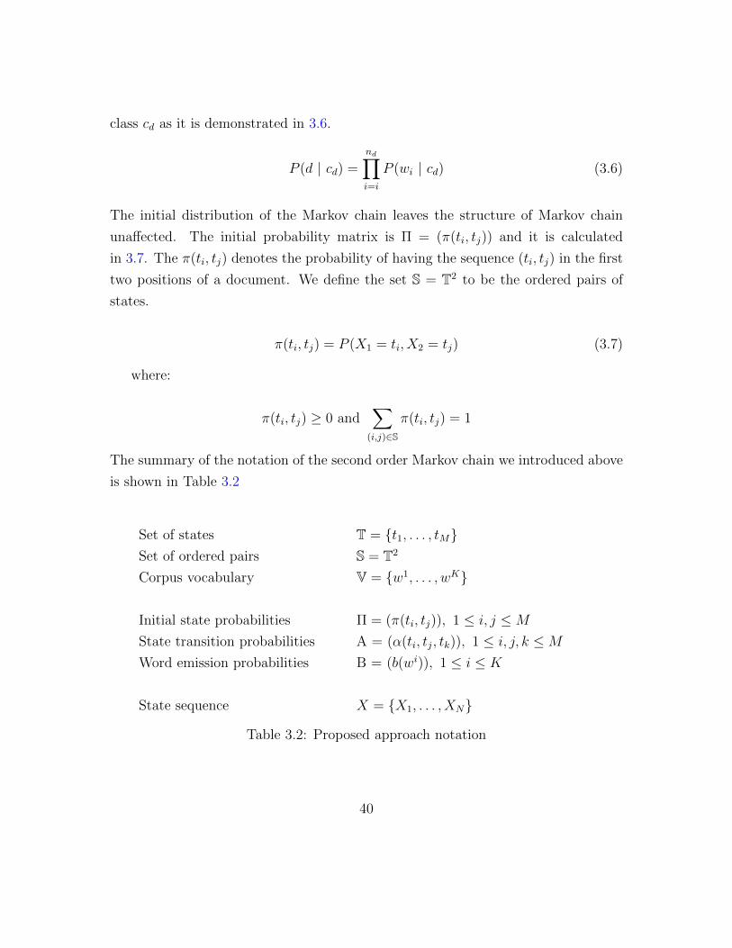
class cd as it is demonstrated in 3.6.
P (d | cd) =
nd∏i=i
P (wi | cd) (3.6)
The initial distribution of the Markov chain leaves the structure of Markov chain
unaffected. The initial probability matrix is Π = (π(ti, tj)) and it is calculated
in 3.7. The π(ti, tj) denotes the probability of having the sequence (ti, tj) in the first
two positions of a document. We define the set S = T2 to be the ordered pairs of
states.
π(ti, tj) = P (X1 = ti, X2 = tj) (3.7)
where:
π(ti, tj) ≥ 0 and∑
(i,j)∈S
π(ti, tj) = 1
The summary of the notation of the second order Markov chain we introduced above
is shown in Table 3.2
Set of states T = {t1, . . . , tM}Set of ordered pairs S = T2
Corpus vocabulary V = {w1, . . . , wK}
Initial state probabilities Π = (π(ti, tj)), 1 ≤ i, j ≤M
State transition probabilities A = (α(ti, tj, tk)), 1 ≤ i, j, k ≤M
Word emission probabilities B = (b(wi)), 1 ≤ i ≤ K
State sequence X = {X1, . . . , XN}
Table 3.2: Proposed approach notation
40

The following described models posit two classes of document d, C = {on, off}. The
models ignore any topic fluctuations, thus each single document discuss a sole topic,
which is either ‘on’ or ‘off’. Any contingent topic transitions may result to ‘off’ clas-
sification. The models are trained to recognize ‘on’ documents only. The documents
not recognized as ‘on’ are considered to be ‘off’.
In fact, a document class depends on a range of factors like the topic distribution,
the context, et cetera. As stated, we posit that the document class depends solely on
the sequence of the states and the emission of the words. The algorithm takes advan-
tage of the class labels of the annotated documents and regards that the document
collection is generated only by considering that the employed words are influenced
by the two previous states. We refer to the introduced set of models with the name
Markovian Topic Identifiers (MTI).
The MTI are not ordinary topic classifiers since they are trained on instances of the
same class. They are trained on the “experience” of the dataset that discusses the
topic of our interest and they are employed to resolve whether an unknown document
is ‘on’ or ‘off’ the given topic. Shortly, they perform one-class classification since
they solely “learn” the properties of the ‘on’ topic and they are not trained on ‘off’
topics as binary classifiers require to perform.
The MTI models provide an exploratory analysis of the impact of different proper-
ties of word to recognize topics based on the semantics of the input. For example,
in subsection 3.5.1, we investigate the impact of stopwords in topic detection; thus
we consider two classes of words. One that reflects the stopwords and the other, the
rest of the vocabulary. Several other models are introduced in the following section.
41

3.5 Word Groups Constitution
The primary objective of this process is to form groups of words that are data-
representative. The language sequential models that treat words as atomic units
suffer from sparsity [15]. Thus, in several different works [13], words are treated in
terms of clusters regarding a common role they exhibit. For instance, verb and nouns
words are studied to “unveil their semantic roles” [22] . The labor that it is needed
to train a statistical system to understand language is significantly reduced [22] since
fewer classes are considered compared to language models where each single word is
a class itself [15].
In this work, we form sets of words by following heuristic criteria exploring their
efficacy as prior knowledge on topic recognition. The sets are formed considering
linguistic components [59] i.e structural1 or content2 words.
We apply two different methods to form the word groups. Firstly, by manually
crafted (Subsection 3.5.1) the word sets and secondly by an explanatory analysis
of the dataset regarding different statistical measures (Subsection 3.5.2) that rank
terms regarding their “importance” to the topic class.
3.5.1 Manually Crafted Word Groups
The Role of Stopwords
This model explores the role of stopwords that topic models ignore [9] and Shoaib
[53] claims that “It is not clear the role that the stopwords play in topic modeling”.
Here, we define two groups, one consists of the stopwords and the other consists of
the content words of the document. The stopwords for the English language come
1Or functional are the words that convey a short lexical meaning and their main goal is to holdthe sentences together
2Or lexical words words have meaning(s) i.e., nouns, verbs
42
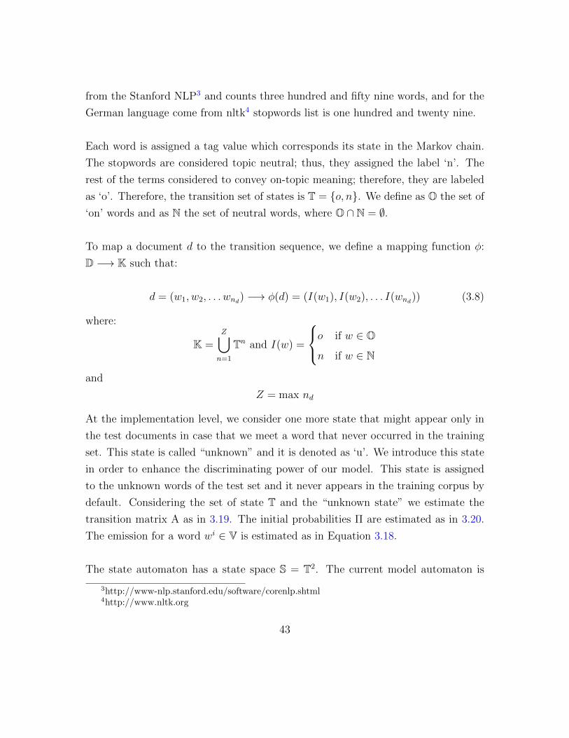
from the Stanford NLP3 and counts three hundred and fifty nine words, and for the
German language come from nltk4 stopwords list is one hundred and twenty nine.
Each word is assigned a tag value which corresponds its state in the Markov chain.
The stopwords are considered topic neutral; thus, they assigned the label ‘n’. The
rest of the terms considered to convey on-topic meaning; therefore, they are labeled
as ‘o’. Therefore, the transition set of states is T = {o, n}. We define as O the set of
‘on’ words and as N the set of neutral words, where O ∩ N = ∅.
To map a document d to the transition sequence, we define a mapping function φ:
D −→ K such that:
d = (w1, w2, . . . wnd) −→ φ(d) = (I(w1), I(w2), . . . I(wnd
)) (3.8)
where:
K =Z⋃
n=1
Tn and I(w) =
o if w ∈ O
n if w ∈ N
and
Z = max nd
At the implementation level, we consider one more state that might appear only in
the test documents in case that we meet a word that never occurred in the training
set. This state is called “unknown” and it is denoted as ‘u’. We introduce this state
in order to enhance the discriminating power of our model. This state is assigned
to the unknown words of the test set and it never appears in the training corpus by
default. Considering the set of state T and the “unknown state” we estimate the
transition matrix A as in 3.19. The initial probabilities Π are estimated as in 3.20.
The emission for a word wi ∈ V is estimated as in Equation 3.18.
The state automaton has a state space S = T2. The current model automaton is
3http://www-nlp.stanford.edu/software/corenlp.shtml4http://www.nltk.org
43

illustrated in Figure 3.2. If S = {S1, · · ·Sn} is the set of nodes of the state automa-
ton and E = {E1, · · · En} its set of edges, then, ∀ Si, Sj ∈ S, Si → Sj /∈ E. This
means that we need to calculate a subset of all possible connection of the nodes of
the automaton. For example, there is not a directed edge between Si = (n, n) and
Sj = (o, o) nodes because the probability of such a transition is zero. This decrease
the number of transition calculations in the model.
On each edge a label of the form P (ti | tj, tk) is assigned that denotes the probability
to meet ti while the two previous states are (tj, tk), where ti, tj, tk ∈ T. The transition,
in this case, is from state (tj, tk) to (tk, ti). For example, the edge E1 : (o, n)→ (n, n)
has a probability P (n | o, n) to occur. We refer to this model as Stopwords Model.
Figure 3.2: State diagram of Stopwords Model
44

3.5.2 Weighting Schemes Crafted Word Groups
In this set of models, we rely on a weighting schemes to constitute the initial groups
of words, we consider in our model. In literature exist several word selection methods
for dimensionality reduction that are important for tasks like clustering and docu-
ment classification. Some of the widely used methods are information gain, mutual
information and chi-square. As described in a comparative study by Yang et al.
[60] all of the previously mentioned methods are calculated in conjunction with the
classification classes. They rely on formulas that weight the words regarding to at
least two classes. In this work, we propose a system that relies only on one-class
documents. Thus, we need weighting schemes that are class independent. As a
rather promising approach [10, 49] that relies on the word frequency and the corpus
size, we use Term Frequency (TF)-Inverse Document Frequency (IDF) to extract the
“important” words and form groups of words.
TF-IDF Weighting Schema
The TF - IDF [50] was introduced as a weighting factor that reflects the “importance”
of a word w in a document d. For each word, the word frequency is calculated and
the inverse frequency of the word in the corpus D it is contained is also computed
according to the formula:
TFIDF (w, d,D) = TF (w, d)× IDF (w,D) (3.9)
where TF is the logarithmically scaled word frequency defined as:
TF (w, d) = log(f(w, d) + 1) (3.10)
and the IDF scale factor for the “importance” of the word:
IDF (w,D) = log|D|
|d ∈ D : w ∈ d|(3.11)
TF-IDF is designed to attenuate the effect of terms that occur very often in a col-
lection of documents. TF-IDF scales down the term frequency of a word w by the
45

reversed metric of the total number of documents containing the term w. TF-IDF is
used as an “importance” measure of the words in a collection of documents. In our
case, higher TF-IDF score implies higher topic importance.
The Role of TF-IDF
In this model, we use three sets of words. One is crafted by the stopwords and it
is denoted as N. The second consists by the first thousand most important words
with respect to TF-IDF ranking and is denoted by F and the third set is the rest of
the input vocabulary; denoted as O. The previously defined sets are pairwise disjoint.
The set of states of the Markov model is T = {f , n, o} for the F, N and O respectively.
The TF-IDF is applied on the input dataset to rank the words regarding the input
documents. In this case, TF-IDF provides us with a ranked list of the words that
are considered to be important for the topic of our interest.
We define a mapping function φ: D −→ K that maps a document d to the transition
sequence as follows:
d = (w1, w2, . . . wnd) −→ φ(d) = (I(w1), I(w2), . . . I(wnd
)) (3.12)
where:
K =Z⋃
n=1
Sn and I(w) =
f if w ∈ F
n if w ∈ N
o if w ∈ O
and
Z = max nd
As in the Stopwords Model, at the implementation level, we consider the “unknown
state” denoted as ‘u’. We need this state in order to enhance the discriminating
power of our model. This state is assigned to the unknown words of the test set
46

and it never appears in the training corpus. Considering the set of state T and
the “unknown state” we estimate the transition matrix A as in 3.19. The initial
probabilities Π are estimated as in 3.20. The emission matrix B is estimated as in
equation 3.18. The set of states for the finite state automaton of this model has a
set of states S = T2. We refer to this model by TF IDF model
The Role of Latent Dirichlet Allocation
In this model, we explore the discriminating power of the introduced sequential model
blended with groups of words produced by latent Dirichlet allocation. Latent Dirich-
let allocation is used to extract the corpus-wide topics of the dataset. It provides
the significant co-occurrent words in the collection sorted into a predefined number
of sets. We explore how the LDA topics fluctuation in the training set can be used
to recognize the input topic on unknown documents.
To extract the corpus-wide topic we utilize the LDA package5 of R. The number of
topics are predefined to three. The total number of words into the three sets is nine
hundred and ninety. LDA topics as illustrated in Figure 1.1 can produce topics that
contain common words. In our case we craft the groups to be pairwise disjoint; we
select two hundred unique words for each set.
On that front, we assume that a word wi ∈ V is assigned a tag value in T =
{p1, p2, p3, n, o}. The p1 to p3 represent the tags for the three topics extracted by
LDA. The tag n is assigned to stopwords and the tag o is assigned to the rest of the
vocabulary. We denote the corresponding sets as P1, P2, P3, N and O respectively.
We define a map function φ that maps a document d to a transition sequence as
follows: φ: D −→ K such that:
d = (w1, w2, . . . wn) −→ φ(d) = (I(w1), I(w2), . . . I(wn)) (3.13)
5https://cran.r-project.org/web/packages/lda/lda.pdf
47

where:
K =Z⋃
n=1
Sn and I(w) =
pi if w ∈ Pi, for 1 ≤ i ≤ 3
o if w ∈ O
n if w ∈ N
(3.14)
and
Z = max nd
We refer to this model as LDA3 Model.
3.6 MTI Training
In this section, we discuss the model inference parameters (Subsection 3.6.2) and
the document classification process of a new document (Subsection 3.6.3). Following
the document classification process we present a way to deal with the classification
boundary identification given that we have calculated the scores of only the on-
topic class documents. At the beginning (Subsection 3.6.1) we discuss the document
representation structure that facilitates the training process.
3.6.1 Document Representation and Pre-processing
Before discussing the inference and learning of the models parameters and the docu-
ment classification formalization it is important to discuss how a document is repre-
sented. The standard in statistical NLP and machine learning is the feature vector.
Feature vector provides the ability to deal with different text objects like words,
sentences et cetera. It facilitates the test of various hypothesis using different math-
ematical frameworks. The common BoW representation considers a document as a
probability distribution of words for a given vocabulary. In this case, a feature vec-
tor is a set of unique words its one assigned a positive real number lower than one,
which represents a probability. Other options exist where instead of a probability
the frequency or a boolean value that denotes the word existence occur. Generally,
a feature vector can contain several feature like the document length or other infor-
48

mation related to the text.
Our representation retain the entire collection of documents as it is. The fundamental
idea is to store each document in a form of tri-grams to facilitate the mathematical
calculations. For instance the document: “The unemployment rate was projected”
is represented in the form of trigrams as: {[The, unemployment, rate], [unemploy-
ment, rate, was], [rate, was projected]}. This technique is used in other domains
like speech recognition or language modeling. The trigram representation although
requires more storage capacity eases the implementation of the model.
Moreover, we discard any punctuation of the source text and convert all words in
lower case. Since we are interested of the word sets fluctuations and not the word
fluctuations itself; our approach is not influenced by the different forms of the same
word stems because they exhibit high probability to co-exist in the same predefined
groups.
3.6.2 Inference and Learning
The models described in 3.5.1 and 3.5.2 rely on a Markov chain. To infer the model
parameters we need to calculate the Bayesian statistics of the model. As introduced
in section 3.4 the transition, emission and initial probabilities need to be estimated
on the training set.
The most intuitive way to estimate probabilities is the Maximum Likelihood Es-
timation (MLE). The MLE estimations are frequents counts normalized to receive
values between zero and one. For a fixed set of observed data, MLE parameter values
provide the maximum probability of the training corpus. The MLE estimators are
denoted with the ˆ symbol to discriminate from probability values.
The training data consists of documents where each document d = (w1, . . . , wnd)
is paired with the hidden state sequence φ(d) = (I(w1), I(w2), . . . I(wnd)) provided
49

by the φ: D −→ K function of each model, where I(wi) ∈ T. We define N(wi)
and N(tk, tj, ti) the number of times the word wi is observed in the corpus and the
number of times the hidden sequence (ti, tj, tk) has been observed in the training
corpus respectively.
Given the above definitions, the maximum likelihood estimates are:
b(wi) =N(wi)∑
wi∈VN(wi)
(3.15)
a(ti, tj, tk) =N(ti, tj, tk)∑
tk∈TN(ti, tj, tk)
(3.16)
and
π(ti, tj) =|{d ∈ D | (I(w1), I(w2)) = (ti, tj)}|
|D|(3.17)
The a(ti, tj, tk), b(wi) and π(ti, tj) do not consider events that are not present in the
training corpus making the probability of observed events the higher it can be. In
NLP, even if we use a large training collection of documents, it is very likely that in
the test corpus we meet words unseen in the training corpus. The MLE assign zero
probabilities to unseen words/states or combinations of them; these zeros will prop-
agate through the multiplication of subparts probabilities ending up to bad classifiers.
To resolve the issues that arise from data sparseness, we need to assign some proba-
bility mass to unseen events. Therefore, we utilize a smoothing method to consider
some probability mass for events never occurred in the training set. One simple way
to smooth the probabilities is by adding one to zeros and on the other hand, we
reduce the non-zeros ones. In other words, we discount the non-zero probabilities to
get the probability mass that we assign to the zero counts. This method is called
Laplace smoothing [44].
Considering Laplace smoothing we update Formulas 3.15, 3.16 and 3.17 as follows:
50

b(wi) =1 +N(wi)
|V|+∑
wi∈VN(wi)
(3.18)
a(ti, tj, tk) =1 +N(ti, tj, tk)
|T|+∑tk∈T
N(ti, tj, tk)(3.19)
and
π(ti, tj) =1 + |{d ∈ D | (I(w1), I(w2)) = (ti, tj)}|
|S|+ |D|(3.20)
In 3.18 we ensure that unseen words in a test document receive a non-zero proba-
bility. In particular, each unseen word w is assigned P (w) = 1|V| . Smoothing the
generated words is very significant, more than the transitions probabilities since it
might exist many new words that do not emit in the training corpus.
Similarly, in 3.19 we assign a probability mass of P (tk | ti, tj) = 1|T| for each unseen
transition E : (ti, tj)→ (tj, tk). For each unseen pair (ti, tj) of initial probabilities we
assign probability mass of P (ti, tj) = 1|S| as it is provided by 3.20.
3.6.3 Document Classification
The classification of a new unknown document d relies on the two following tasks.
First, we map d to a topic space regarding a score we introduce in this section.
Second, we deduce ‘on’ class for d whether its classification score falls into the clas-
sification boundary created by the topic scores of the training documents.
Usually, in probabilistic binary classification methods we infer about the class of
document d according to the probabilities of d to belong c1 or c2 class. The class
cd ∈ {c1, c2} is the class where P (cd | d) is maximized:
P (cd | d) = max{P (c1 | d), P (c2 | d)}
51

In our model, we can not use the probability as a classification measure since we
train our system in solely one class. Instead, we use a topic score that is derived
directly from the posterior probability P (cd = on | d), which is the probability of the
document d to belong to class cd = on.
To achieve the classification of d = (w1, w2, . . . , wnd) into two classes C = {on, off },
we need the corresponding φ function, φ: D −→ K for each model introduced in 3.5.1
to 3.5.2 that maps the document d into the sequence of states φ(d). The probability
of d to be ‘on’ given the transition sequence φ(d) is P (cd = on | d). Using Bayes
rule, P (cd = on | d) is estimated as follows:
P (cd = on | d) ∝ P (d | cd = on)
where:
P (d | cd = on) = π(I(w1), I(w2)) ∗ b(w1) ∗ b(w2)
nd∏i=3
a(I(wi−2, I(wi−1), I(wi)) ∗ b(wi)
(3.21)
We logarithm over 3.21 and normalize dividing by document length to yield length
independent scores. We refer to the above-introduced score as Logarithmic Topic
Score (LTS).
LTS =
log(π(I(w1), I(w2)) ∗ b(w1) ∗ b(w2)) +nd∑i=3
[log(a(I(wi−2), I(wi−1), I(wi))) + log(b(wi))]
nd
(3.22)
We believe that documents of the same topic yield scores concentrated around a lim-
ited area. Documents that exhibit high frequency of words the are not in the training
set, we forsee, to have high LTS score because we assign a small emission probability
to unknown words. Documents that have vocabularies close to the training set but
of different topic we expect to have different fluctuation of the Markov states, thus
52

values located on different areas of input corpus. In the next subsection 3.6.4 we
introduce the method that we determine the topic boundary.
3.6.4 Classification Boundary Identification
In this section, we handle the issue of identifying a classification boundary given the
value space of only one class of documents. We want to identify the bounding values
of the LTS topic score distribution of the training corpus.
In literature two approaches have been proposed to address one-class classification
problems. In 1999 Scholkopf et al. [52] extended SVM to deal with solely one-class
instances. Scholkopf proposed a way to identify a boundary given data of one class.
First, they use a kernel function to map data to a feature space F and then they
setup an optimization problem in which they separate the mapped data from the
origin using the conventional support vector machines technique. The classification
function returns +1 in a confined region where the training data points are located
and -1 elsewhere.
In 2004 Dax et al. [20] proposed a method that provides a hyperspherical boundary
in feature space that surrounds the training data points. The spherical classification
boundary is described by a center α and a radius R. The center is a linear com-
bination of support vectors and the distance of all data points from the center is
less than R. The soft margin penalized technique (Subsection 2.2.2) is used for data
points where the distance is greater than R. This problem is an optimization problem
where they minimize the outliers effect.
Practically, to specify the topic boundary we use the e1071 library or R-project which
implements the LIBSVM [16] library of SVM. The implementation of e1071 library
follows Scholkopf’s implementation [52] The tolerance of the boundary to outliers is
determined by the ν parameter, where ν ∈ (0, 1). The lower value ν receives, the
53

fewer outlier ratio it exhibits as is depicted in 3.3.
Figure 3.3: Boundary variation on different ν values
54

Chapter 4
MTI Evaluation
4.1 Data Acquisition
In this thesis, we obtain data for three different evaluation scenarios. We gather
documents that discuss the topic that we train our model. This consists the gold
standard dataset. Some more datasets are obtained to evaluate the discriminating
power of our model that exhibit low and high vocabulary overlapping to the gold
standard dataset.
4.1.1 Federal Reserve Datasets
We download documents from Federal Reserve Bank (FED) of the United States.
FED is the central bank of the USA and its main goals are to provide the USA
with a safer, more flexible, and more stable monetary and financial system. The
first corpus is called Federal Reserve Open Market Committee (FOMC) and it is the
gold standard document that we train our model. The second dataset we collect
comes also from FED and it is called Beige Book. We select these datasets because
they are in well written English, they are issued by the same institute and they both
lay on the same domain. They discuss different financial aspects concerning the US
economy and we assume that regardless their different themes that maybe exist in,
55

each collection discusses one particular topic.
Federal Open Market Committee Corpus
The emphasis of the gold standard dataset is on a particular topic. We download
FOMC documents between the years 2007 and the end of 2014. The gold standard
comprises the official releases of the Federal Open Market Committee of Federal Re-
serve concerning the monetary policy decision in the United States. These reports
are released eight times per year. Furthermore, it comprises the corresponding meet-
ing Minutes that include personalized statements and further policy details released
three weeks after the date of the policy decision. In addition to FOMC, an Eco-
nomic Projection is issued to supplement FOMC releases four times annually. The
data include charts and figures that are not subject to this work. The number of
the documents that consist the gold standard dataset is one hundred and fifty eight.
The dataset is downloaded from the official website1 of the Federal Reserve Bank of
the United States.
Beige Book Corpus
The second collection of documents is used to evaluate the performance of our model
in the case that we have documents of the same domain. This dataset consisting
of the Beige Book summaries. The Beige Book summaries are released two weeks
before FOMC meetings and eight times per year exposing anecdotal information
about the current economic conditions in its District sourced by banks, economists,
market experts et cetera. This corpus consists of brief and extended reports for each
event from 2007 and the end of 2014. The corpus counts one hundred and twelve
documents downloaded from the official website of FED.
1http://www.federalreserve.gov/monetarypolicy/default.htm
56

4.1.2 American National Corpus
The third dataset is the generic Manually Annotated Sub-Corpus (MASC) corpus
part of the Open American National Corpus (OANC) downloaded from the official
website2. It is a balanced collection of mainly written texts of half million words
of contemporary American English. It is comprised of nineteen different genres
of text discussing different topics. The corpus has been manually annotated by
the authors for logical structure, tokenizations and part-of-speech, name entities et
cetera. OANC and MASC rely on contributions of data from various linguistics
and NLP communities. The genres distribution is demonstrated in Table 4.1. The
number of documents of MASC is three hundred and ninety.
Genre No. words Pct corpus
Court transcript 30052 6%
Debate transcript 32325 6%
Email 27642 6%
Essay 25590 5%
Fiction 31518 6%
Gov’t documents 24578 5%
Journal 25635 5%
Letters 23325 5%
Newspaper 23545 5%
Non-fiction 25182 5%
Spoken 25783 5%
Technical 27895 6%
Travel guides 26708 5%
Twitter 24180 5%
Blog 28199 6%
Ficlets 26299 5%
Movie script 28240 6%
Spam 23490 5%
Jokes 26582 5%
Table 4.1: MASC topics specification
2http://www.anc.org/
57

4.1.3 HC German Corpora
HC is a German corpus consist of documents of published on three different source,
newspapers, web blogs and twitter. The list of some of the sources and the number
of documents collected from each one of them is depicted in Table 4.33. The corpus
is downloaded from the original source4 preserving only the news items that come
from newspapers and magazines.
The list of documents available from newspapers and magazines are assigned the
code numbers one and two respectively. The dataset contains documents that lay on
twenty-eight different categories assigned specific codes that denote the topic of each
document. Some of the topics of HC corpus are Politics, environment, food, health,
crime & law, travel, arts, sport, science and technology, travel et cetera.
We retrieve the documents that are about health, crime & law, and travel and discard
all the rest. These three categories contain a number of documents that ensure the
statistical significance of our experiments and at the same time the processing time
remains acceptable. The number of documents that we retain for each of the three
topics is shown in Table 4.2.
Topic No. of document
Health 1150
Crime & Law 501
Travel 1138
Table 4.2: HC topics-documents specification
3Downloaded from http://www.corpora.heliohost.org/statistics.html4http://www.corpora.heliohost.org/
58

Source No. of document
spiegel.de 4931
sueddeutsche.de 1251
tagesspiegel.de 1104
muensterschezeitung.de 1611
abendblatt.de 3461
stern.de 3143
zeit.de 2775
welt.de 3517
handelsblatt.com 1159
kn-online.de 126
rp-online.de 4265
focus.de 831
faz.net 4396
ruhrnachrichten.de 1567
noz.de 4595
augsburger-allgemeine.de 3567
ln-online.de 142
derwesten.de 1061
an-online.de 3912
badische-zeitung.de 229
jungewelt.de 517
haz.de 571
fazfinance.net 4021
az-web.de 3908
neues-deutschland.de 4662
taz.de 635
blogger.de 7935
blogmonster.de 5353
twitter.com 947774
Table 4.3: HC corpus sources
59
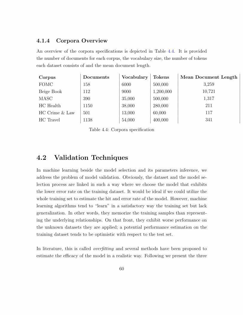
4.1.4 Corpora Overview
An overview of the corpora specifications is depicted in Table 4.4. It is provided
the number of documents for each corpus, the vocabulary size, the number of tokens
each dataset consists of and the mean document length.
Corpus Documents Vocabulary Tokens Mean Document Length
FOMC 158 6000 500,000 3,259
Beige Book 112 9000 1,200,000 10,721
MASC 390 35,000 500,000 1,317
HC Health 1150 38,000 280,000 211
HC Crime & Law 501 13,000 60,000 117
HC Travel 1138 54,000 400,000 341
Table 4.4: Corpora specification
4.2 Validation Techniques
In machine learning beside the model selection and its parameters inference, we
address the problem of model validation. Obviously, the dataset and the model se-
lection process are linked in such a way where we choose the model that exhibits
the lower error rate on the training dataset. It would be ideal if we could utilize the
whole training set to estimate the hit and error rate of the model. However, machine
learning algorithms tend to “learn” in a satisfactory way the training set but lack
generalization. In other words, they memorize the training samples than represent-
ing the underlying relationships. On that front, they exhibit worse performance on
the unknown datasets they are applied; a potential performance estimation on the
training dataset tends to be optimistic with respect to the test set.
In literature, this is called overfitting and several methods have been proposed to
estimate the efficacy of the model in a realistic way. Following we present the three
60

methods that are widely used to validate supervised machine learning algorithms
with respect to a particular dataset.
Hold-Out Validation
A common approach is the hold-out method where the training set is split into two
disjoint sets where one of them is used to train the model and the other to estimate
its performance and it is called test set (Figure 4.1). Usually, the training set pos-
sesses the higher proportion of the training set since sufficient number of samples
need to be fed to the algorithm for its parameters to be estimated properly. The
proportion of the training set might be split into two third and one third for the
learning and the test set respectively. In practice, different proportions can be used
depending on the size of the training set and the complexity of the model.
Figure 4.1: Holdout validation method
Hold-out exhibits two significant shortcomings. Considering the learning curve in
Figure 4.2, where the model accuracy increases with the size of the training set, the
hold-out efficacy estimation is pessimistic since only a part of the of the training set
is used for model training. Moreover, it may happen that the learning set proportion
is not sufficiently representative deriving a misleading efficacy estimation. This is
due to the fact that the hold-out method relies on a singular split of the train and
test set.
61

Figure 4.2: Learning curve of different learners on text data [2]. It demonstrates therising accuracy performance as the training set is increasing.
Cross Validation
In k-fold cross-validation, the training set S is partitioned in k disjoint equal sized
folds S1, S2, . . . Sk. The validation is repeated k times and for each iteration one of the
k folds is used for validation and the rest k-1 is used for learning. For each iteration
i ∈ {1, 2, . . . k} the algorithm is trained on S\Si and tested on Si as is illustrated in
Figure 4.3, for k = 5. The supervised method efficacy is estimated on every of the k
subsamples. Practically, the validation is performed on the entire training set and the
error rate is the average of the errors on the k iterations [40] as shown in equation 4.1
eavg =1
k
k∑i=1
ei (4.1)
The advantage of cross-validation compared with the hold-out method is that the
whole set is used for training and testing. In this setting we avoid inappropriate
splits that lead to inaccurate performance estimations that are too pessimistic for
the model. The average error estimation provides us with more realistic efficacy
62

estimation.
Figure 4.3: Cross-validation method with five folds. Each iteration uses the one fifthof the data for testing. The five folds are equally sized and disjoint.
63

An important point concerning k-fold cross validation is the criteria that we choose
the value of k. In general, it is a trade-off between efficacy estimation and compu-
tational time. In case that k is large, the bias of the error estimate is small and
the efficacy assessment is pragmatic. On the other hand, the computational time to
perform more iteration is expensive considering that some of the machine learning
models exhibit high computational complexity. In case that k is small, the bias of
the error is higher and the estimator is conservative. Apparently, the iterations are
less and the computational time is reduced.
In general, the choice of the number of cross-validation iterations is practically cor-
related with the size of the dataset. For large datasets, even three iterations could
provide sufficiently accurate error estimates, but more iterations are needed on sparse
datasets to receive an accurate estimation. The commonly used value for k is ten;
the test set on each iteration is the ten percent of the entire training set then.
Leave-One-Out Validation
Leave-one-out is analogous to cross-validation. In a set of N training samples, N-1 are
used for the learning phase and one for efficacy estimation. The process is repeated
N times since all the dataset samples are used for testing. In this extreme case of
cross-validation, the error estimate is unbiased but it could exhibit high variance.
Moreover, the computational cost is the highest since the number of folds is equal
to the number of training instances. For each fold, a new model has to be trained
making this validation method slow.
This approach is suitable when there is not sufficient number of data or they are not
properly distributed in order to be split into training and test set as in conventional
validating approaches. Ultimately, it is sensible to use five or ten-fold cross validation
since they appear to be quite effective in practice.
64

4.3 Evaluation Measures
In literature different evaluation methods have been developed to measure the per-
formance of classification systems. In this section, we present several measures that
can be used on binary classification to measure the efficacy of the positive and neg-
ative samples or of the entire test set. All of the classification measures we present
in this section are based on a confusion matrix as it is illustrated in table 4.5
act
ual
valu
e
Prediction outcome
total
TruePositive
FalseNegative
P
FalsePositive
TrueNegative
N
Table 4.5: Confusion matrix
The binary classification performance is described by a number of measures that facil-
itate the performance estimation based on different statistical observations. Firstly,
we describe what the values true positive/negative and false positive/negative rep-
resent in table 4.6.
In table 4.7 we summarize the most important measures. We denote X and X the
random variables for the class and the prediction respectively. We refer to the true
positives as TP, the true negatives as TN, the false positives as FP and the false
negatives as FN. The positive samples are P and the negatives are N, the positive
and negative class is ⊕ and respectively.
65
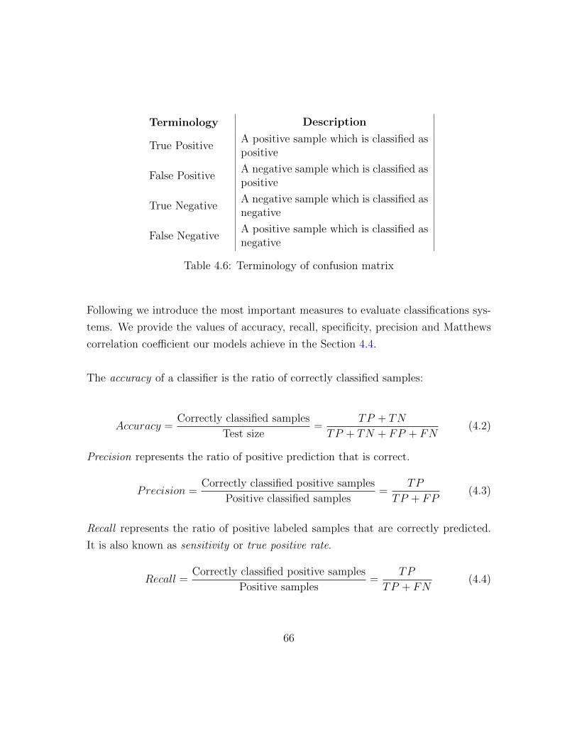
Terminology Description
True PositiveA positive sample which is classified aspositive
False PositiveA negative sample which is classified aspositive
True NegativeA negative sample which is classified asnegative
False NegativeA positive sample which is classified asnegative
Table 4.6: Terminology of confusion matrix
Following we introduce the most important measures to evaluate classifications sys-
tems. We provide the values of accuracy, recall, specificity, precision and Matthews
correlation coefficient our models achieve in the Section 4.4.
The accuracy of a classifier is the ratio of correctly classified samples:
Accuracy =Correctly classified samples
Test size=
TP + TN
TP + TN + FP + FN(4.2)
Precision represents the ratio of positive prediction that is correct.
Precision =Correctly classified positive samples
Positive classified samples=
TP
TP + FP(4.3)
Recall represents the ratio of positive labeled samples that are correctly predicted.
It is also known as sensitivity or true positive rate.
Recall =Correctly classified positive samples
Positive samples=
TP
TP + FN(4.4)
66

Specificity represents the ratio of negative labeled samples that are correctly pre-
dicted.
Specificity =Correctly classified negative samples
Negative samples=
TN
TN + FP(4.5)
False positive rate (FPR) represents the ratio of negative labeled samples that are
misclassified as positive.
FPR =Correctly classified negative samples
Negative samples=
FP
FP + TN(4.6)
F1 score is the harmonic mean of precision and recall. It receives values F1 ∈ [0,1],
where 1 is the best score and 0 is the worst. Good classification algorithms maximize
precision and recall simultaneously. In general, a classifier that exhibits a moderate
good performance on both is favored over overly high performance on only one of
them.
F1 = 2 · precision · recallprecision+ recall
(4.7)
Matthews Correlation Coefficient (MCC) [43] is a quality measure of a binary clas-
sification. It returns the correlation coefficient between the actual and the predicted
class values. The coefficient value MCC ∈ [-1,1]. MCC = -1 is the worst value MCC
receives since it denotes a total discrepancy between the actual and the predicted
values. MCC = 1 denotes a perfect concordance between the actual and the pre-
dicted values. MCC = 0 denotes a prediction not superior to the random classifier5.
The advantage of MCC is that it can be used even if the two classes possess different
proportion whereas metrics like accuracy, precision, recall, specificity etc are mis-
leading if they are not contrasted with random classifier predictions. MCC is also
known as phi coefficient.
5A random classifier is the classifier that predicts always according to the class that possessesthe higher proportion in the training set
67

MCC =TPN− S · P√
P · S(1− S)(1− P )(4.8)
where:
N = TN + TP + FN + FP ,
S =TP + FN
N,
P =TP + FP
N
Metric Description Estimation
Accuracy P(X = X) ACC = TP+TNP+N
Precision P(X = ⊕ | X = ⊕) PREC = TPTP+FP
Recall or Sensitivity P(X = ⊕ | X = ⊕) REC = TPP
Specificity or TruePositive Rate
P(X = | X = ) SPEC = TNN
False Positive Rate P(X = ⊕ | X = ) FPR = FPN
MCC6 or Phi Coeffi-cient
Returns a classification qualitymeasure with respect to randomclassifier.
MCC = TP ·TN−FP ·FN√P ·(TP+FP )·(TN+FN)·N
F1 ScoreRepresents the harmonic mean ofprecision and recall.
F1 = 2 · precision·recallprecision+recall
Rate of Positive Pre-dictions
P(X = ⊕) RPP = TP+FPP+N
Rate of Negative Pre-dictions
P(X = ) RNP = TN+FNT+N
Table 4.7: Classification performance measures
6MCC returns a value C ∈ [-1,1]. C = 0 implies a random prediction. C = 1 implies a perfectprediction. C < 0 implies a worse than random prediction
68

4.4 Results
In this section we proceed to the MTI (Chapter 3) evaluation results. We propose
three evaluation scenarios the outcome of which we discuss subsequently. The first
scenario evaluates the Stopwords Model, TF IDF Model and LDA3 Model of Sub-
section 3.5.1 and 3.5.2 in comparison with two widely used binary classifiers NB and
SVM presented in Section 2.2. The datasets the three models discriminate are the
FOMC and the MASC corpus presented in Subsection 4.1. In the second scenario,
our models are evaluated on the FOMC and Beige Book corpora. The Markovian
topic identifiers are compared with NB and SVM as in the first scenario. In the third
scenario, Stopwords Model and TF IDF Model are evaluated on two subcases to ex-
plore their performance on German language and on other than financial documents.
We conduct two tests, one the HC Health against the HC Crime & Law corpus and
the other the HC Health corpus against the HC Travel corpus. In both cases, the
on-topic documents are the ones of the health topic.
In both experimental scenarios we take into account the following evaluation metrics:
Precision, recall, accuracy, specificity and MCC introduced in Table 4.7. All the tests
are conducted using a ten-fold cross-validation method presented in Subsection 4.2.
We choose the precision (PREC) and recall (REC) measures for our models because
we are interested in the percentage of positive predictions that are correct and the
the percentage of positive labeled instances that were predicted as positive. We ex-
amine how our models deal with the recognition of on-topic documents since they are
trained on them. Furthermore, we calculate the specificity of our models to explore
how accurately our model discard off-topic documents.
The MCC is used because it is a comparison coefficient between the proposed model
and the default classifier. In our case the compared corpora are unbalanced, so the
default classifier achieves accuracy higher than fifty percent. MCC provides us with
a numerical value of how much better our classifier is regarding the default classi-
69

fier. The accuracy (ACC) provides the proportion of predictions that are correct but
it should be interpreted in contradistinction with the default classifier performance
otherwise it can be misleading.
As it was presented in Subsections 3.6.4 a classification boundary is calculated given
the topic scores LTS of the training collection. To do so the one class SVM method
is used [52]. The selection of the ν (Subsection 3.6.4) value is important since it
dramatically influence the classification performance. When 0.1 ≤ ν ≤ 0.3 we notice
that we achieve high accuracy values in all the scenarios. In particular, in the ma-
jority of the scenarios when ν = 0.3, we achieve the highest performance values. To
keep it uniform we select ν = 0.3 for all scenarios, since even if we do not reach the
highest performance values we are close to them. The selection of ν = 0.3 does not
change the rank of the performance of MTI models in each scenario.
The classification tasks and the processing steps of the algorithms were implemented
in R-project and some corresponding CRAN [55] libraries that implement different
classification, evaluation and plotting tools. Weka7 was used to apply the baseline
classifications of NB and SVM. Weka [61] provides an easy and convenient environ-
ment to perform plenty of data mining and machine learning tasks. It is an open
source framework implemented in Java that provides, among the implementation of
popular algorithms, other pre-processing and manipulation tools and graphic repre-
sentation facilities.
4.4.1 Evaluation Classifiers Selection
In both experimental scenarios, we compare our models performance with the base-
line results provided by the other two classifiers, NB and SVM. In literature exist
several other classifiers that are used for text classification. We select the multi-
nomial NB because it is a primitive classifiers than rely solely on the bag-of-words
7Weka stands for Waikato Environment for Knowledge Analysis
70
representation without the utilization of extra weighting methods or optimizations.
It uses only the emissions of the words given the class to discriminate between the
two classes. The MTI models rely also on the emissions (Subsection 3.6.2) with the
extra property of the word sequences provided by the transitions (Subsection 3.6.2).
NB provides in our case the “ground zero” to study our research questions 1 and 2
presented in Section 1.3.
The selection of SVM as the second baseline classifier is preferred since it is effective
in text classification [35] providing an upper bound of the efficiency of our models.
SVM are effective in text classification since they provide zero weight to the words
that do not contribute to discrimination and weights the terms that support the
classification process (support vectors). In its soft margin version, they penalize the
missclassified terms and using the kernel trick (Subsection 2.2.2). they exhibit high
discriminating efficiency.
Having a baseline comparison framework in one’s disposal we can identify how well
our models perform. The baseline performance of NB and SVM facilitates a com-
parison between the baseline provided results and the efficiency of the introduced
models preserving the same input. Herein, the aspect of evaluating the topic recog-
nition performance of the Markovian topic identifiers is examined. The topic recog-
nition is evaluated in terms of classification performance between ‘on’ and ‘off’ topic
instances.
4.4.2 Experimental Scenario I
In this scenario, we evaluate the performance of Stopwords model, TF IDF model
and LDA3 Model as described in Section 3.5 on the two dataset that discusses dif-
ferent topics. The dataset we train our model is the FOMC dataset that has a clear
financial orientation (Section 4.1). The topic of FOMC documents is the monetary
policy in the USA. The topic of FOMC is the one we intend to recognize.
71

The dataset that we use to evaluate our model in conjunction with FOMC is the
MASC corpus. It is a generic dataset that discusses several topics covering different
domains. We examine the efficacy of our method on “learning” the ninety percent
of FOMC and recognize it among the rest ten percent set of FOMC and the entire
MASC corpus documents in a single iteration of a cross-validation setup.
We consider this as the “easy” case since the topics of the two collections are clearly
different and lay on different domains. Thus, in this scenario we use as baseline
classifiers NB and SVM, as discussed in 4.4.1, to be the “ground zero” of our models
performance estimation.
Classifier PREC REC ACC(%) SPEC MCC Kernel
NB 0.90 0.90 99.4 1 0.90 —
SVM 0.90 0.90 99.2 0.90 0.90 Radial
Stopwords Model 1 0.81 99.2 1 0.90 —
TF IDF Model 1 0.83 99.3 1 0.91 —
LDA3 Model 1 0.63 98.5 1 0.79 —
Table 4.8: Classification results - Experimental scenario I
At a first glance of the models accuracy in Table 4.8 we realize that all of them
classify with high accuracy, greater than ninety-eight percent. MCC shows that the
majority of methods perform much better that the default classifiers since MCC
value is close to one. The MCC value of LDA3 Model is significantly lower that
all the other models. The reason is that its recall REC = 0.63 is low. Considering
Stopwords Model and TF IDF Model we notice that both reach with efficacy on this
scenario.
The precision (PREC) and specificity (SPEC) of Stopwords Model, TF IDF Model
and LDA3 Model is one. In other words the percentage of positive predictions that
72

are correct is one hundred percent; and the percentage of negative labeled instances
that are predicted as negative is one hundred percent respectively. This means that
our models don’t have false positive but they exhibit a number of false negatives.
In absolute number, one to five documents are miss-classified as negative in the first
two proposed models during the ten-fold cross-validation iterations. For LDA3 Model
the number of miss-classified documents are three to seven. In Tables A.1, B.1
and C.1 are exposed the numbers of documents classified in each iteration. A rea-
son for that might be a miss-classification error of one-class SVM and/or the lack
of enough samples for the proposed models to unveil properly the FOMC structure.
Taking into consideration the values of precision and specificity we realize that our
models can miss-classify a positive sample but they never miss-classify a negative
sample. In other words the resulted positive classified documents discuss the topic
of our interest.
4.4.3 Experimental Scenario II
In this scenario, we evaluate the performance of Stopwords Model, TF IDF Model
and LDA3 Model on the two datasets that discuss different topics but lay on the
same domain. The two datasets are the FOMC, that discuss the monetary policy
in the US, and the Beige Book. Both of them have clear financial orientations and
issued by Federal Reserve Bank.
We consider this as the “difficult” case since the topics of the two collection fall into
the same domain. As previously we use as baseline classifiers NB and SVM to be
provided with “ground zero” performance of two widely used methods on text. As
we can see in Table 4.9, NB exhibits an accuracy of fifty-eight percent, which is ap-
parently poor. It classifies as bad as the random classifier does since MCC measure is
zero. The reason is that in NB the entire vocabulary contributes to the classification
of the two corpora of similar terminology.
73

On the other hand SVM classification accuracy rockets to more than ninety-nine
percent. The reason for this is that support vector machines classify regarding a
subset of the training set. In particular, it identifies the words (support vectors)
that have some discriminating power and weights zero to the rest of the vocabulary.
The MCC classification performance of SVM is close to one which means an almost
perfect efficacy compared to the default classifier.
Classifier PREC REC ACC(%) SPEC MCC Kernel
NB 0.34 0.58 58.4 0 0 —
SVM 0.99 0.99 99.6 0.99 0.99 Radial
Stopwords Model 1 0.66 95.8 1 0.79 —
TF IDF Model 1 0.82 97.7 1 0.90 —
LDA3 Model 1 0.64 95.6 1 0.78 —
Table 4.9: Classification results - Experimental scenario II
As in experimental Scenario I of Subsection 4.4.2 the precision (PREC) and speci-
ficity (SPEC) of Stopwords Model and TF IDF Model is one. This means that our
models do not have false positive but they have a number of false negatives. In
absolute numbers three to eight documents are miss-classified as negative in the
Stopwords Model during the ten-fold cross-validation iteration (Table A.2) and one
to four for TF IDF Model (Table B.2). For LDA3 Model the miss-classified docu-
ment are three to nine as depicted in Table C.2 Considering the values of precision
and specificity we realize that our models can miss-classify a positive sample but they
never miss-classify a negative sample.This means that the resulted positive classified
documents discuss the topic of our interest.
Comparing the three proposed methods we realize that TF IDF Model outperforms
Stopwords Model and LDA3 Model. In particular, the accuracy is better (about
74

ninety-eight instead of about ninety-six percent of the other two models) and the re-
call of TF IDF Model is twenty five percent higher that the one of Stopwords Model
and LDA3 Model. The MCC measure indicates again that the TF IDF Model clas-
sifies better that other two proposed models with respect to the default classifier.
4.4.4 Experimental scenario III
In this scenario we evaluate the performance of Stopwords model and TF IDF model
as described in Section 3.5 on a different language than English and different domains
that finance. We conduct two experiments, both on German language but different
topics. In the first experiment we train our model on HC Health corpus against the
HC Crime & Law corpus, the specifications of them are presented in Table 4.4. We
discard LDA3 Model since it exhibits lower discriminating performance than Stop-
word Model and TF IDF Model.
In the second experiment, we evaluate the performance of HC Health corpus against
HC Travel corpus (Table 4.4). In the following two subsections, we discuss the effi-
cacy of our models by the measurements provided in Tables 4.10 and 4.11.
Health versus Crime & Law
Classifier PREC REC ACC(%) SPEC MCC
Stopwords Model 0.82 0.79 93 0.96 0.76
TF IDF Model 0.75 0.78 91.1 0.94 0.71
Table 4.10: Experimental Scenario III - Health vs Crime & Law
At a first glance of the models performance in Table 4.10 we realize that both models
exhibit high accuracy greater than ninety percent. The MCC value indicates that
75

both classify significantly better than default classifier since both values are signifi-
cantly higher than zero. Comparing Stopwords Model and TF IDF Model we notice
that the former performs slightly better in contrast to scenarios I and II.
The recall values are very close to both models, slightly lower than 0.8. As in scenar-
ios I and II, a number of false negatives exist; in other words about eighty percent of
the ‘on’ instances are predicted correctly. What it is different regarding the scenario
I and II is that in this case we have a number of false positives; this means that a
proportion of eighty-two percent and seventy-five percent of the ‘on’ classified docu-
ments are correct in Stopwords Model and TF IDF Model respectively.
The precision values exhibit some difference, since Stopwords Model is nine percent
higher than TF IDF Model and both, are close to one. This means that a num-
ber of false positives exist when dealing with the German language. In contrast, in
scenarios I and II the number of false positives was zero. Furthermore, Specificity
rockets close to one for both models which means that as in scenarios I and II our
proposed models are very effective on the percentage of correctly classified ‘off’ docu-
ments since its higher than ninety-four percent for both models. We notice the same
in scenarios I and II since both reach the highest value of precision. The absolute
numbers of miss-classifications can be seen in Tables A.3 and B.3).
Health versus Travel
Classifier PREC REC ACC(%) SPEC MCC
Stopwords Model 0.76 0.79 95.8 0.97 0.75
TF IDF Model 0.76 0.70 95.2 0.98 0.70
Table 4.11: Experimental Scenario III - Health vs Travel
In Table 4.11 we observe that both models have accuracy values that are close and
76

greater than ninety-five percent. The MCC value indicates that both classify signif-
icantly better than default classifier since both values are apparently greater than
zero. Comparing Stopwords Model and TF IDF Model we notice that the former
performs slightly better in contrast to scenarios I and II.
The precision values are identical and lower than 0.8. In other words a number of false
positives exist as in the previous experiment of HC Health versus HC Crime & Law.
Likewise, we realize that our models exhibit a significant number of false positives
when dealing with the German language. The recall values are different. In partic-
ular, Stopwords Model has twelve percent higher recall value than TF IDF Model.
In contrast to the first two experimental scenarios where recall is one, a significant
number of false negatives exist.
Specificity rockets close to one for both models. Similarly, as in scenarios I and II our
proposed models can effectively discard ‘off’ documents since specificity is greater
than ninety-seven percent for both models. We observe the same in scenarios I and
II since both reach the highest value of precision. The absolute numbers of miss-
classifications can be seen in Tables A.4 and B.4).
4.4.5 Word Order Impact on Topic Recognition
In this chapter, we perform an exploratory analysis of the impact of word order on
topic recognition. We essentially study the research question three we pose in Sec-
tion 1.3. We conduct a number of experiments to prove that the topic of a collection
of documents is bound to a particular word order. As Wallach depicted in her work
[56] the documents A, B “the department chair couches offers” [56] and “the chair
department offers couches” respectively exhibit the same word statistics but convey
different topics. We are motivated by this example to prove that shuffling the words
in the documents of a corpus we come up with several other topics.
77
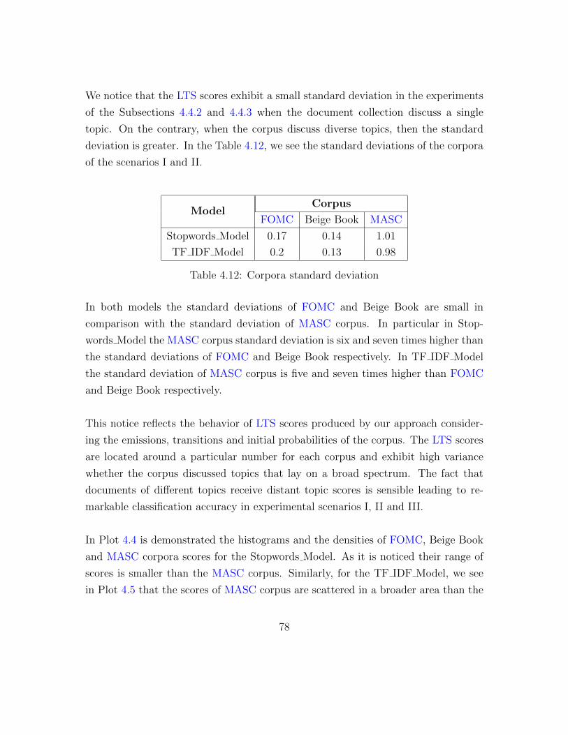
We notice that the LTS scores exhibit a small standard deviation in the experiments
of the Subsections 4.4.2 and 4.4.3 when the document collection discuss a single
topic. On the contrary, when the corpus discuss diverse topics, then the standard
deviation is greater. In the Table 4.12, we see the standard deviations of the corpora
of the scenarios I and II.
ModelCorpus
FOMC Beige Book MASC
Stopwords Model 0.17 0.14 1.01
TF IDF Model 0.2 0.13 0.98
Table 4.12: Corpora standard deviation
In both models the standard deviations of FOMC and Beige Book are small in
comparison with the standard deviation of MASC corpus. In particular in Stop-
words Model the MASC corpus standard deviation is six and seven times higher than
the standard deviations of FOMC and Beige Book respectively. In TF IDF Model
the standard deviation of MASC corpus is five and seven times higher than FOMC
and Beige Book respectively.
This notice reflects the behavior of LTS scores produced by our approach consider-
ing the emissions, transitions and initial probabilities of the corpus. The LTS scores
are located around a particular number for each corpus and exhibit high variance
whether the corpus discussed topics that lay on a broad spectrum. The fact that
documents of different topics receive distant topic scores is sensible leading to re-
markable classification accuracy in experimental scenarios I, II and III.
In Plot 4.4 is demonstrated the histograms and the densities of FOMC, Beige Book
and MASC corpora scores for the Stopwords Model. As it is noticed their range of
scores is smaller than the MASC corpus. Similarly, for the TF IDF Model, we see
in Plot 4.5 that the scores of MASC corpus are scattered in a broader area than the
78

Figure 4.4: Stopwords Model scores histograms and densities
other two datasets.
Hypothesis Testing
We believe that by randomly permuting the words in the documents of a single-topic
collection, we produce a permuted corpus that discusses more than one topic as in
the documents “the department chair couches offers” [56] and “the chair department
offers couches” [56] of Wallach. The obtained collection we expect to have a larger
variance of scores as MASC corpus exhibits.
To explore the impact of word order on topic identification we introduce a statistical
hypothesis testing. We calculate later how likely it is a higher standard deviation to
occur on the permuted corpora. Given that the null hypothesis is true, we accept or
79

Figure 4.5: TF IDF Model scores histograms and densities
reject it with respect to the standard deviations of the permutations. We introduce
the following null hypothesis:
1. Null hypothesis (H0): The order of the words in documents does not affect the
topic(s) of the corpus.
The null hypothesis is rejected if the p-value which is the probability under the null
hypothesis is less than the significance level of s0 = 0.05. This means that at least
ninety five percent of the permuted corpora should have a greater standard deviation
than the initial corpus (unpermuted).
We conduct the permutations experiments on the Beige book which exhibits the
smallest standard deviation in the TF IDF Model. We perform a number of P per-
mutations, which in our case is one hundred, on a random sample of ten percent of
the beige book corpus. The p-value is the probability that the permuted corpora
80

have lower standard deviation than the original one. The p-value is calculated as in
Equation 4.9.
pval = 1− |{sdi > sd0, 1 ≤ i ≤ P}|P
(4.9)
where:
P = 100
The histogram and densities of the standard deviations of the permuted corpora are
illustrated in Figure 4.6. The red perpendicular line represents the standard devia-
tion of the source corpus from where the permutations were derived. The permuted
corpora standard deviations are located rightmost of the red line at their majority.
The p-value is calculated to be pval = 0.5.
Figure 4.6: Beige Book permutations distribution
The evidence of p-value is equal to the significance level s0 which means that the H0
is rejected at the s0 level of significance. Thus, we accept the alternative hypothesis
H1.
2. Alternative hypothesis (H1): The order of the words affects the topic(s) of the
81

corpus.
One reason for receiving scores of high standard deviations might be the fact that
the permuted documents in each corpus contain a sequence of words that never ex-
ist in human written language. Thus, they are assigned very low probabilities in
the transitions calculated on the training set. This could influence significantly the
standard deviation of a corpus. Considering the groups of words we utilize in the
permutation tests only a sequence of stopwords is unusual to occur in reality.
To assure that this is not the reason for the low received p-value that led us to accept
the alternative hypothesis H1, we conduct an experiment of ten permutations on the
ten percent of randomly selected documents of the MASC dataset that has a wider
diversity of topics. We receive nine standard deviations greater than the original
corpus and one that it is lower than the original one as it is depicted in Plot 4.7.
The red line represents the original collection of documents standard deviation value.
Figure 4.7: MASC permutations distribution
In case that the reason for the nine highly standard deviated corpora is the abnormal
82

consecutive stopwords then the consecutive stopwords distribution of the only low
standard deviated corpus would be different of the nine highly standard deviated
corpora. We calculate the correlation of the stopwords duplet, triplet, quadruplet,
quintuplet et cetera vector of the one against the other nine others. The values we
receive are all close to one as it is shown in Table 4.13. Perm 1 is the permutation
one that exhibits lower standard deviation than the source. With Perm 2 to 10, we
denote the rest nine permutations with standard deviations higher than the source.
Perm 2 Perm 3 Perm 4 Perm 5 Perm 6 Perm 7 Perm 8 Perm 9 Perm 10
Perm 1 0.9998980 0.9999799 0.9999417 0.9999158 0.9999560 0.9999321 0.9999692 0.9997212 0.9999321
Table 4.13: Permutation correlations
For the calculation of the correlations of Table 4.13 we use Pearson correlation that
makes no assumptions about the distributions of the population. Pearson correlation
[47] measures is a correlation measure providing the linear dependence between two
variables X and Y . It outputs +1 in case of a perfect positive correlation, 0 in case
of no correlation and -1 in a perfect negative correlation.
As a result, we point out that in the low standard deviated permuted corpora, the
stopwords sequences are not distributed differently than the nine others. Therefore,
stopwords effect is not the reason for the low p-value. It is due to the fact that by
permuting the words in a document we receive more topics as Wallach [56] claimed
with her example in 2006: Document A: “the department chair couches offers” [56]
can be permuted to document B: “the chair department offers couches” whereas
documents A and B discuss different topics.
83

Chapter 5
Summary
5.1 Conclusions
This research work presents a stochastic process to recognize documents of a par-
ticular topic. The primary motivation stems from an assumption coherent with
probabilistic topic models. Their inference relies on the bag-of-words representation
of documents; only the word and their frequencies are considered in the model. We
introduce an approach based on high order Markovian chains to capture the natural
language semantics inherent in the sequence of words.
The MTI are supervised topic models since they consider the human background
to infer about the model parameters. They are oriented to recognize similar to the
training corpus document structures; in this way they discriminate a document as
‘on’ or ‘off’ topic. Their discriminating power is based on the premise that docu-
ments of the same topics follow the same patterns. Following infrequent to the input
patterns leads to distant to the on-topic documents scores. The models are trained
on the experience of one class input thus they need less effort than usual binary
classifiers that require data for both the wanted and unwanted situations.
In this thesis, we figure out that the introduced topic identifiers exhibit a satisfactory
84

performance on several different scenario, different domains and languages compared
to other popular topic classifiers. In experimental scenarios I and II in Section 4.4 we
notice that the MTI compete for classifiers that rely on bag-of-words representation.
MTI perform as effective as NB and SVM in scenario I; they approach the perfor-
mance of SVM and overstep NB in scenario II. MTI performance is satisfactory in
the German language as well. Considering the research question one as defined in
Section 1.3 we deduce that the stochastic topic identifiers can perform satisfactorily
on discriminating text of different domains and languages.
MTI are fused with prior knowledge in terms of groups of words with common char-
acteristics. It is shown that the stochastic model that relies on TF-IDF weight-
ing scheme exhibits a supreme performance in comparison to the other stochas-
tic models introduced in experimental scenario I and II. On the other hand, the
Stopwords Model exhibits supreme performance in the German language in sce-
nario III although the performance of TF IDF Model competes for the one of Stop-
words Model. A reason for this may be the special characteristics of each language.
Accordingly, to answer the research question two in Section 1.3 we need to conduct
more experiments.
Moreover, in this thesis we experiment the inter-correlation of topic and word se-
quence and we conclude that word order impacts the topic of a document (research
question three in Sections 1.3). Granted that we define a topic as the model that
best fits what humans consider as a topic, we are provided the terrain to study the
impact of word restructuring on topic modulation since the topic of a document is
reflected in a particular score area. We strengthen in this way the intuition that
humans have as it is depicted in Wallach work [56]; we may produce a new topic by
simply restructuring the words of a passage. To put it in a different way, the order
of the words is selected in a concrete way to convey the authors topic. We conclude
that the documents produced by restructuring the word sequence convey different
topics.
85

In conclusion, the MTI models exhibit a number of strengths compared to other topic
identification and classification methods that rely on the bag-of-words paradigm. We
highlight the advantages and potentials of the introduced models in the following
points:
• MTI models require small training datasets to be effective. Not only due to the
fact that they recognize a topic by unveiling the structure of only same topic
documents but also because they consider a set of words to reduce the number
of the possible transitions manipulating data sparsity. Both considerations
make MTI cost performance efficient.
• In MTI pre-processing steps are not required. Probabilistic topic models and
conventional classifiers require the feature vector of word frequencies to per-
form. The construction of such a vector adds extra computational cost to the
bag-of-words models. Not to mention the extra pre-processing steps that are
required to increase their effectiveness i.e., word stemming. In MTI the doc-
uments are represented in their original form and special pre-processing steps
like stemming is not necessary to be implemented since words with the same
stem may occur in the same set of words.
• MTI can be used on interdisciplinary fields and on different applications. The
proposed models rely on learning the common patterns of the training collection
of documents which is reflected on the probability values. MTI models may
be used to recognize the writing style of a person since it is characterized by
a particular vocabulary and a manner the words are structured. Moreover,
they may be used on image topic identification. The key point is to define in
a proper way how the word and the document are reflected on an image. A
reasonable way is to consider that the pixels block are the words and an image
is a document. The aspect of the multidimensionality of images with respect
to a document needs to be addressed because a picture element is featured
by many dimensions itself. Consequently, the application and the parameters
estimation of MTI on images need further studies to be achieved.
86

• MTI models capture fine-grained topic semantics. MTI models as it is shown
in the experimental scenario II may be used to perform a more fine-grained
analysis of topics that lay on the same domain; a scenario where a robust
classifier like naıve Bayes exhibit poor performance. In particular, MTI exhibit
high accuracy on discriminating documents of financial domain as shown. MTI
meet the requirements of retrieving documents that have a particular theme or
discuss a particular subject. i.e., the sovereign debt crisis in Europe.
• MTI models are closer to the human semantic representation than bag-of-
words models. Human perception and cognition embrace human memory to
infer about the gist of text [24]. Topic categorization includes not only the
memorization of words but also the manner words are linked. Besides, the
personal interpretation and conception which is challenging to model, word
order contributes to topic identification mechanism. Although MTI models do
not address questions that lay into cognitive science, they simulate to some
extend the topic categorization learning. The usefulness of such systems may
assist firstly, in better understanding human learning processes and secondly,
in the development of better classification models that mimic human brain.
5.2 Shortcomings and Future Work
The MTI models proposed in this thesis exhibit some shortcomings that could lead
to some interesting future research. In the following points, we summarize some
weaknesses our approach exhibits.
• MTI models are language dependent. They adhere to the word order to calcu-
late a score and classify a document as ‘on’ or ‘off’ topic. They are tested on
English and German language and exhibit a remarkable discriminating perfor-
mance. Nevertheless, some languages like Greek and Russian allow flexibility
in the order of the words while preserving the same syntax, thus the same topic.
The generalization of MTI models on any language requires further studies.
87

• MTI models are expensive in both time and space. The MTI models have a
large number of parameters that need to be estimated. In large corpora of
millions of tokens it is computationally demanding to train and validate its
performance in a ten-fold validation scenario. Moreover, the input of our mod-
els is not the conventional vector space but the entire collection of documents
retaining the word order of the documents.
Finally, in the next points, we provide some extensions and future research based on
the fundaments provided in this thesis.
• The MTI models can be extended and tested with different parameters and
prior knowledge. Firstly, MTI models can be extended to incorporate the
emissions of bigrams and trigrams in order to deal effectively with common
collocations like fiscal deficit or White House. This provides more realism to
the model since in domain-oriented documents several n-gram may appear.
The way in which a bigram or a trigram phrase will be selected instead of a
uni-gram, may be achieved either by incorporating a set of usual n-grams or
by an exploration analysis of the corpus based on statistical measures - i.e.,
c-value [21] - to detect n-grams.
• The MTI Markov chains can be extended to incorporate longer memory. We
can introduce Markovian topics identifiers to rely on higher order Markov
chains. It is feasible in this case to deal with the sparsity of data without
dramatically increase the volume of the training set, but just adjusting the
content and the number of sets of words used. This allows models that perform
topic identification at the sentence level. In this way, we can study whether
processing text at a higher level - i.e sentence level - affects topic identification.
This may lead us to the development of more sophisticated models.
• The MTI can recognize topics in a dynamic manner. MTI models are trained
on a fixed set of documents to infer whether an unknown document is ‘on’ or
88

‘off’ topic. MTI can be designed to incorporate “knowledge” that they miss
by updating their parameters without being trained again on the whole. In
this way they maximize their performance based on the feedback from the
environment as the time goes by. The complex of such a model is high and
requires sophisticated techniques to make MTI modular. This topic learning
approach may imply some human external assistance to be maintained simpler.
• The MTI could be language independent. As mentioned in Section 5.2, MTI
rely on the word order to infer about a topic. In some languages like the Greek
one can convey a particular topic by changing in several ways the sequence of
the words. MTI are not designed to capture these details since they stick to
the word order. We might design a language independent stochastic model by
incorporating syntactical knowledge to relax the word order strictness of our
approach.
89

Appendices
90

Appendix A
Stopwords Model
A.1 FOMC - MASC Corpora
Iteration TP TN FP FN
1 14 390 0 2
2 12 390 0 3
3 13 390 0 3
4 14 390 0 2
5 12 390 0 4
6 14 390 0 2
7 12 390 0 4
8 13 390 0 3
9 12 390 0 4
10 13 390 0 2
Table A.1: Stopwords Model ten-fold cross validation performance on FOMC -MASC corpora
91

A.2 FOMC - Baige Book Corpora
Iteration TP TN FP FN
1 12 112 0 4
2 13 112 0 3
3 11 112 0 5
4 12 112 0 4
5 10 112 0 6
6 11 112 0 5
7 10 112 0 6
8 11 112 0 4
9 8 112 0 8
10 7 112 0 8
Table A.2: Stopwords Model ten-fold cross validation performance on FOMC - BeigeBook corpora
92

A.3 HC German Corpus (Health - Crime & Law)
Iteration TP TN FP FN
1 93 481 20 23
2 90 482 19 25
3 88 482 19 27
4 92 481 20 23
5 90 481 20 25
6 99 481 20 17
7 89 483 18 25
8 94 482 19 20
9 93 482 19 22
10 87 483 18 28
Table A.3: Stopwords Model ten-fold cross validation performance on HC Health -HC Crime & Law corpora
93

A.4 HC German Corpus (Health - Travel)
Iteration TP TN FP FN
1 89 1111 27 26
2 93 1109 29 22
3 89 1111 27 24
4 86 1113 25 30
5 91 1109 29 24
6 89 1110 28 27
7 90 1110 28 26
8 92 1108 30 24
9 94 1111 27 21
10 94 1110 28 19
Table A.4: Stopwords Model ten-fold cross validation performance on HC Health -HC Travel corpora
94

Appendix B
TF IDF Model
B.1 FOMC - MASC Corpora
Iteration TP TN FP FN
1 12 390 0 4
2 15 390 0 1
3 12 390 0 3
4 13 390 0 3
5 15 390 0 1
6 14 390 0 2
7 15 390 0 1
8 11 390 0 5
9 13 390 0 3
10 11 390 0 4
Table B.1: TF IDF Model ten-fold cross validation performance on FOMC - MASCcorpora
95

B.2 FOMC - Baige Book Corpora
Iteration TP TN FP FN
1 13 112 0 3
2 11 112 0 4
3 15 112 0 1
4 12 112 0 4
5 14 112 0 2
6 12 112 0 4
7 12 112 0 3
8 12 112 0 4
9 15 112 0 1
10 13 112 0 3
Table B.2: TF IDF Model ten-fold cross validation performance on FOMC - BeigeBook corpora
96

B.3 HC German Corpus (Health - Crime & Law)
Iteration TP TN FP FN
1 94 471 30 21
2 95 472 29 21
3 79 472 29 37
4 97 471 30 17
5 77 470 31 39
6 89 471 30 26
7 96 472 29 17
8 93 471 30 21
9 91 471 30 24
10 91 472 29 25
Table B.3: TF IDF Model ten-fold cross validation performance on HC Health - HCCrime & Law corpora
97

B.4 HC German Corpus (Health - Travel)
Iteration TP TN FP FN
1 76 1111 26 39
2 84 1113 24 31
3 85 1111 26 31
4 89 1111 26 25
5 70 1114 23 45
6 80 1111 26 36
7 75 1113 24 39
8 81 1111 26 34
9 79 1113 24 36
10 86 1111 26 29
Table B.4: TF IDF Model ten-fold cross validation performance on HC Health - HCTravel corpora
98
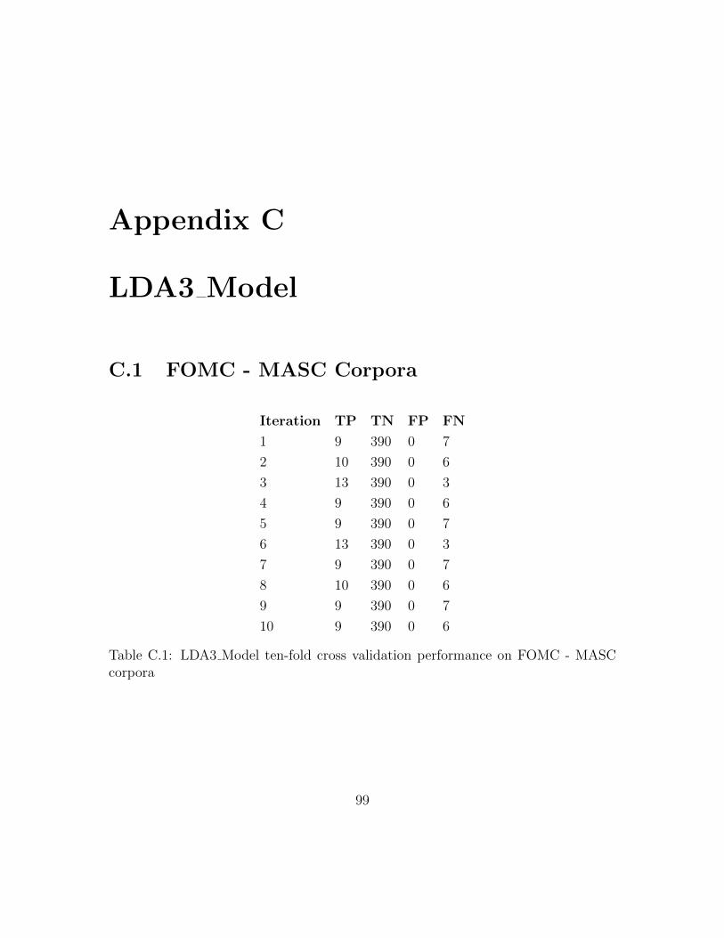
Appendix C
LDA3 Model
C.1 FOMC - MASC Corpora
Iteration TP TN FP FN
1 9 390 0 7
2 10 390 0 6
3 13 390 0 3
4 9 390 0 6
5 9 390 0 7
6 13 390 0 3
7 9 390 0 7
8 10 390 0 6
9 9 390 0 7
10 9 390 0 6
Table C.1: LDA3 Model ten-fold cross validation performance on FOMC - MASCcorpora
99

C.2 FOMC - Baige Book Corpora
Iteration TP TN FP FN
1 12 112 0 4
2 12 112 0 4
3 9 112 0 7
4 9 112 0 7
5 8 112 0 7
6 12 112 0 4
7 11 112 0 5
8 10 112 0 6
9 6 112 0 9
10 13 112 0 3
Table C.2: LDA5 Model ten-fold cross validation performance on FOMC - BeigeBook corpora
100

Bibliography
[1] M. Andrews and G. Vigliocco. The Hidden Markov Topic Model: A Probabilistic
Model of Semantic Representation. Topics in Cognitive Science, pages 101 – 113,
2009.
[2] M. Banko and E. Brill. Scaling to Very Very Large Corpora for Natural Language
Disambiguation. Proceeding ACL ’01 Proceedings of the 39th Annual Meeting
on Association for Computational Linguistics, pages 26–33, 2001.
[3] M. W. Berry, S. T. Dumais, and G. W. O’Brien. Using Linear Algebra for
Intelligent Information Retrieval. SIAM Review, 37(4):573–595, 1995.
[4] D. M. Blei. Probabilistic topic models. Communication of the ACM, 55:77–84,
2012.
[5] D. M. Blei and J. D. Lafferty. Correlated Topic Models. Proceedings of the 23rd
International Conference on Machine Learning, pages 147–154, 2006.
[6] D. M. Blei and J. D. Lafferty. Dynamic topic models. Proceedings of the 23rd in-
ternational conference on Machine learning (ICML 2006), pages 113–120, 2006.
[7] D. M. Blei and J. D. McAuliffe. Supervised Topic Models. Neural Information
Processing Systems, pages 121–128, 2008.
[8] D. M. Blei and P. J. Moreno. Topic Segmentation with an Aspect Hidden
Markov Model. In Proceedings of the 24th Annual International ACM SIGIR
Conference on Research and Development in Information Retrieval, pages 343
– 348, 2001.
101

[9] D. M. Blei, A. Y. Ng, and M. I. Jordan. Latent Dirichlet Allocation. Journal
of Machine Learning Research, 3(4-5):993–1022, 2003.
[10] N. Bloom. Using Natural Language Processing to Improve Document Catego-
rization with Associative Networks. In Proceedings of the 17th International
Conference on Applications of Natural Language Processing and Information
Systems, pages 177–182, 2012.
[11] Booth and T. L. Sequential Machines and Automata Theory. New York: John
Wiley and Sons, Inc, 1est edition, 1967.
[12] J. Boyd-Graber and D. M. Blei. Syntactic Topic Models. Advances in Neural
Information Processing Systems, pages 185–192, 2009.
[13] P. F. Brown, P. V. DeSouza, R. L. Mercer, Pietra, J. Vincent, Della, Lai, and
C. Jenifer. Class-based N-gram Models of Natural Language. Computational
Linguistics, 18, 1992.
[14] P. Bruza, D. Song, and K. Wong. Aboutness from a commonsense perspective.
Journal of the American Society for Information Science, 51(12):1090–1105,
2000.
[15] C. Buck, K. Heafield, and B. van Ooyen. N-gram counts and language models
from the common crawl. In Proceedings of the Language Resources and Evalu-
ation Conference, 2014.
[16] Chang, Chih-Chung, and L. Chih-Jen. LIBSVM: A library for support vector
machines. ACM Transactions on Intelligent Systems and Technology, 2(3):27:1–
27:27, 2011.
[17] W. Darling and F. Song. Syntactic Topic Models for Language Generation.
Neural Information Processing Systems, pages 1–5, 2013.
[18] S. Deerwester, S. T. Dumais, G. W. Furnas, T. K. Landauer, and R. Harsh-
man. Indexing by latent semantic analysis. Journal of the American Society for
Information Science, 41:391–407, 1990.
102

[19] A. Dempster, N. Laird, and D. Rubin. Maximum likelihood from incomplete
data via the EM algorithm. Journal of the Royal Statistical Society, 39(1):1–38,
1977.
[20] D. Fisher. Support Vector Data Description. Journal of Machine Learning,
54:45–66, 2004.
[21] K. T. Frantzi, S. Ananiadou, and J.-i. Tsujii. The C-value/NC-value Method of
Automatic Recognition for Multi-Word Terms. In Proceedings of the Second Eu-
ropean Conference on Research and Advanced Technology for Digital Libraries,
pages 585 – 604, 1998.
[22] D. Gildea. Probabilistic Models of Verb-Argument Structure. In Proceedings
of the 19th International Conference on Computational Linguistics - Volume 1,
pages 1–7, 2002.
[23] G. Y. Gillian Brown. Discourse Analysis. (Cambridge textbooks in linguistics),
1983.
[24] T. L. Griffiths, T. J. B., and S. Mark. Topics in semantic representation. Psy-
chological Review, 114, 2007.
[25] T. L. Griffiths, M. I. Jordan, J. B. Tenenbaum, and D. M. Blei. Hierarchical
Topic Models and the Nested Chinese Restaurant Process. Advances in Neural
Information Processing Systems, pages 17–24, 2004.
[26] T. L. Griffiths, M. Steyvers, D. M. Blei, and J. B. Tenenbaum. Integrating
topics and syntax. Advances in neural information processing systems, 17:537–
544, 2005.
[27] A. Gruber, M. Rosen-Zvi, and Y. Weiss. Hidden topic Markov models. Pro-
ceeding of the International Conference on Artificial Intelligence and Statistics,
pages 163–170, 2007.
103

[28] A. Gruber, Y. Weiss, and M. Rosen-zvi. Hidden Topic Markov Models. In
Proceedings of the Eleventh International Conference on Artificial Intelligence
and Statistics (AISTATS-07), pages 163 – 170, 2007.
[29] L. R. Herrmann. Laplacian-isoparametric grid generation scheme. Journal of
the Engineering Mechan-ics Division, pages 749–907, 1976.
[30] N. Hiroshi, M. Daichi, and Y. Miyao. Improvements to the Bayesian Topic N
-gram Models. Conference on Empirical Methods in Natural Language Process-
ing, (October):1180–1190, 2013.
[31] B. Hjorland. Towards a theory of aboutness, subject, topicality, theme, domain,
field, content ... and relevance. Journal of the American Society for Information
Science and Technology, 52:774–778, 2001.
[32] C. F. Hockett. Two models of grammatical description. Journal of the Linguistic
Circle of New York, 1958.
[33] T. Hofmann. Probabilistic Latent Semantic Indexing. Proceedings of the 22Nd
Annual International ACM SIGIR Conference on Research and Development in
Information Retrieval, pages 50–57, 1999.
[34] T. Hofmann, J. Puzicha, and M. I. Jordan. Learning from dyadic data. Advances
in neural information processing systems II, 11:466–472, 1999.
[35] T. Joachims. Text Categorization with Suport Vector Machines: Learning with
Many Relevant Features. In Proceedings of the 10th European Conference on
Machine Learning, pages 137–142, 1998.
[36] T. Joachims. Transductive Inference for Text Classification Using Support Vec-
tor Machines. In Proceedings of the Sixteenth International Conference on Ma-
chine Learning, pages 200–209, 1999.
[37] B. H. Juang and L. R. Rabiner. Hidden Markov Models for Speech Recognition.
Technometrics, 33(3):251–272, 1991.
104

[38] N. Kawamae. Supervised N-gram Topic Model. Proceedings of the 7th ACM
International Conference on Web Search and Data Mining, pages 473–482, 2014.
[39] E. O. Keenan and B. Schieffelin. A Reconsideration of Left Dislocation in Dis-
course. Proceedings of the 2nd Annual Meeting of the Berkeley Linguistics So-
ciety, pages 240–257, 1976.
[40] R. Kohavi. A Study of Cross-validation and Bootstrap for Accuracy Estimation
and Model Selection. Proceedings of the 14th International Joint Conference on
Artificial Intelligence, 2(0):1137–1143, 1995.
[41] R. V. Lindsey, W. P. Headden III, and M. J. Stipicevic. A Phrase-Discovering
Topic Model Using Hierarchical Pitman-Yor Processes. Proceedings of the 2012
Joint Conference on Empirical Methods in Natural Language Processing and
Computational Natural Language Learning, (July):214–222, 2012.
[42] C. D. Manning, P. Raghavan, and H. Schutze. An Introduction to Information
Retrieval. Cambridge, 2008.
[43] B. Matthews. Comparison of the predicted and observed secondary structure of
T4 phage lysozyme. Biochimica et Biophysica Acta, 405(2):442–451, oct 1975.
[44] T. Mitchell. Machine Learning. McGraw-Hill, Inc., 1 edition, 1997.
[45] V. P. Mulbregt, I. Carp, L. Gillick, S. Lowe, and J. Yamron. Text segmentation
and topic tracking on broadcast news via a hidden markov model approach.
In The Fourth International Conference on Spoken Language Processing, pages
2519–2522, 1998.
[46] K. Nigam, McCallum, A. Kachites, S. Thrun, and T. Mitchell. Text Classifi-
cation from Labeled and Unlabeled Documents using EM. Journal of Machine
Learning, 39(2-3):103–134, 2000.
[47] K. Pearson. Notes on regression and inheritance in the case of two parents. In
Proceedings of the Royal Society of London, pages 240 – 242, 1895.
105

[48] L. R. Rabiner. A tutorial on hidden Markov models and selected applications
in speech recognition, 1989.
[49] J. Ramos. Using tf-idf to determine word relevance in document queries. In
First International Conference on Machine Learning, 2003.
[50] G. Salton, E. A. Fox, and H. Wu. Extended Boolean Information Retrieval.
Communications of the ACM, 26(11):1022–1036, 1983.
[51] L. Saul and F. Pereira. Aggregate and mixed-order Markov models for statis-
tical language processing. Proceedings of the Second Conference on Empirical
Methods in Natural Language Processing, pages 81–89, 1997.
[52] B. Scholkopf, J. Shawe-taylor, J. C. Platt, A. J. Smola, and R. C. Williamson.
Estimating the Support of a High-Dimensional Distribution. Journal of Neural
Computation, 13:1443–1471, 2001.
[53] J. Shoaib and W. Lam. An Unsupervised Topic Segmentation Model Incorporat-
ing Word Order. Proceedings of the 36th International ACM SIGIR Conference
on Research and Development in Information Retrieval, pages 203–212, 2013.
[54] M. Steyvers and T. Griffiths. Probabilistic topic models. Handbook of latent
semantic analysis, pages 424–440, 2006.
[55] R. D. C. Team. R: A Language and Environment for Statistical Computing. R
Foundation for Statistical Computing, 2008.
[56] H. M. Wallach. Topic Modeling : Beyond Bag-of-Words. Proceedings of the 23rd
International Conference on Machine Learning, pages 977–984, 2006.
[57] C. Wang and B. Thiesson. Markov topic models. International Conference on
Artificial Intelligence and Statistics, 5:583–590, 2009.
[58] X. Wang, A. Mccallum, and X. Wei. Topical N-grams: Phrase and Topic Dis-
covery , with an Application to Information Retrieval. Proceedings of the 2007
Seventh IEEE International Conference on Data Mining, pages 697–702, 2007.
106

[59] E. Winkler. Understanding Language. 2007.
[60] Y. Yang and J. O. Pedersen. A Comparative Study on Feature Selection in Text
Categorization. In Proceedings of the Fourteenth International Conference on
Machine Learning, pages 412–420, 1997.
[61] K. H. Zeileis, C. Buchta, and Achim. Open-Source Machine Learning: R Meets
Weka. Computational Statistics, 24:225–232, 2009.
[62] H. Zhang. The Optimality of Naive Bayes. In Proceedings of the Seventeenth
International Florida Artificial Intelligence Research Society Conference, pages
103–130, 2004.
107