displacement mapping on the gpu — state of the art
TRANSCRIPT
Volume 25 (2006), Number 3 pp. 1–24
Displacement Mapping on the GPU —State of the Art
László Szirmay-Kalos, Tamás Umenhoffer
Department of Control Engineering and Information Technology, Budapest University of Technology, HungaryEmail: [email protected]
AbstractThis paper reviews the latest developments of displacement mapping algorithms implemented on the vertex, geom-etry, and fragment shaders of graphics cards. Displacement mapping algorithms are classified as per-vertex andper-pixel methods. Per-pixel approaches are further categorized as safe algorithms that aim at correct solutions inall cases, to unsafe techniques that may fail in extreme cases but are usually much faster than safe algorithms, andto combined methods that exploit the robustness of safe and the speed of unsafe techniques. We discuss the possibleroles of vertex, geometry, and fragment shaders to implement these algorithms. Then the particular GPU basedbump, parallax, relief, sphere, horizon mapping, cone stepping, local ray tracing, pyramidal and view-dependentdisplacement mapping methods, as well as their numerous variations are reviewed providing also implementationdetails of the shader programs. We present these methods using uniform notations and also point out when dif-ferent authors called similar concepts differently. In addition to basic displacement mapping, self-shadowing andsilhouette processing are also reviewed. Based on our experiences gained having re-implemented these methods,their performance and quality are compared, and the advantages and disadvantages are fairly presented.
Keywords: Displacement mapping, Tangent space, Di-rect3D 9 and 10, HLSL, Silhouettes, Self shadowing, GPU
ACM CCS: I.3.7 Three-Dimensional Graphics and Realism
1. Introduction
Object geometry is usually defined on three scales, themacrostructure level, the mesostructure level, and themicrostructure level. A geometric model refers to themacrostructure level and is often specified as a set of polyg-onal surfaces. The mesostructure level includes higher fre-quency geometric details that are relatively small but stillvisible such as bumps on a surface. The microstructurelevel involves surface microfacets that are visually indis-tinguishable by human eyes, and are modeled by BRDFs[CT81, HTSG91, APS00, KSK01] and conventional tex-tures [BN76, Bli77, CG85, Hec86].
Displacement mapping [Coo84, CCC87] provides highfrequency geometric detail by adding mesostructure prop-
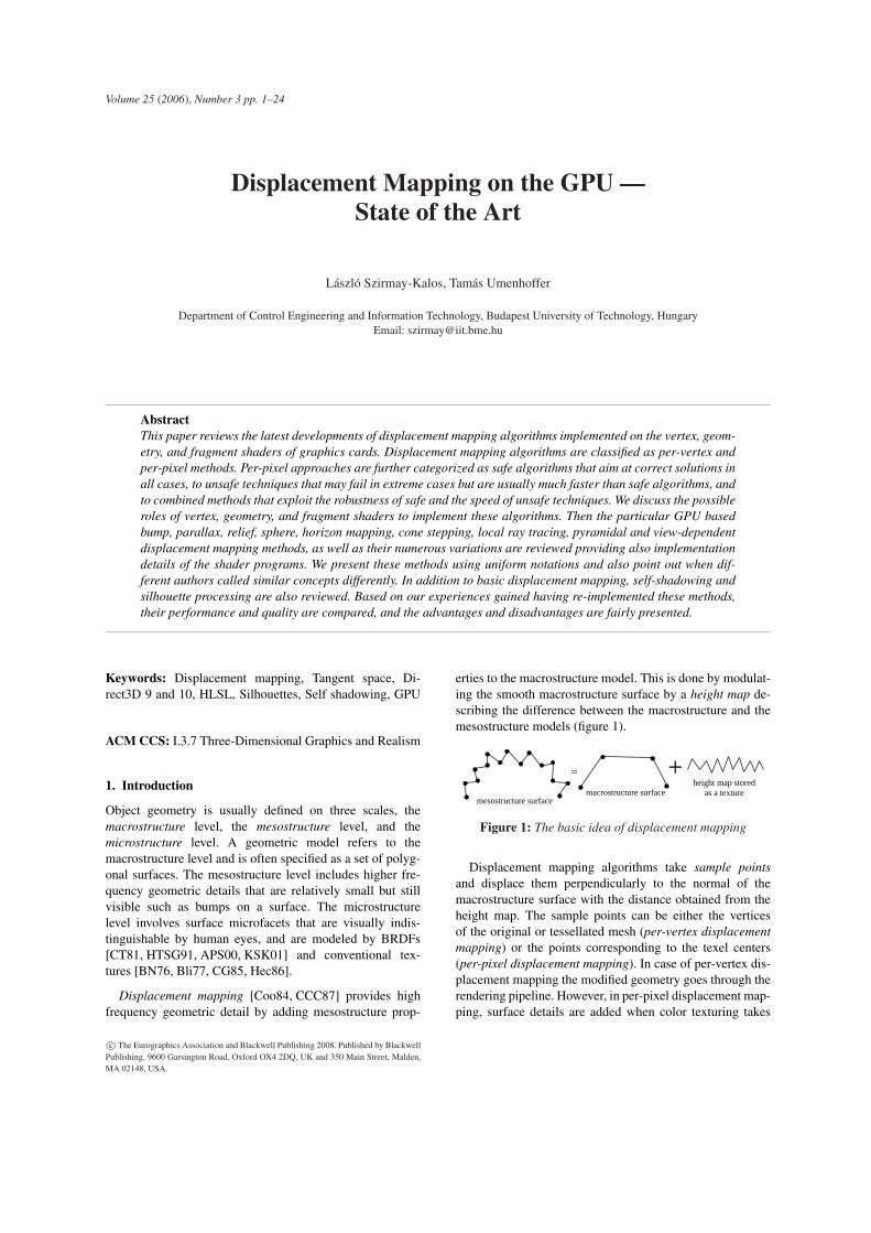
erties to the macrostructure model. This is done by modulat-ing the smooth macrostructure surface by a height map de-scribing the difference between the macrostructure and themesostructure models (figure 1).
mesostructure surfacemacrostructure surface
height map storedas a texture
= +
Figure 1: The basic idea of displacement mapping
Displacement mapping algorithms take sample pointsand displace them perpendicularly to the normal of themacrostructure surface with the distance obtained from theheight map. The sample points can be either the verticesof the original or tessellated mesh (per-vertex displacementmapping) or the points corresponding to the texel centers(per-pixel displacement mapping). In case of per-vertex dis-placement mapping the modified geometry goes through therendering pipeline. However, in per-pixel displacement map-ping, surface details are added when color texturing takes
c© The Eurographics Association and Blackwell Publishing 2008. Published by BlackwellPublishing, 9600 Garsington Road, Oxford OX4 2DQ, UK and 350 Main Street, Malden,MA 02148, USA.
Szirmay-Kalos, Umenhoffer / Displacement Mapping on the GPU
place. The idea of combining displacement mapping withtexture lookups was proposed by Patterson, who called hismethod as inverse displacement mapping [PHL91].
Inverse displacement mapping algorithms became popu-lar also in CPU implementations. CPU based approaches[Tai92, LP95] flattened the base surface by warping andcasted a curved ray, which was intersected with the displace-ment map as if it were a height field. More recent meth-ods have explored direct ray tracing using techniques suchas affine arithmetic [HS98], sophisticated caching schemes[PH96] and grid base intersections [SSS00]. Improvementsof height field ray-tracing algorithms have also been pro-posed by [CORLS96, HS04, LS95, Mus88]. Huamin Qu etal. [QQZ∗03] proposed a hybrid approach, which has thefeatures of both rasterization and ray tracing.
On the GPU per-vertex displacement mapping can be im-plemented by the vertex shader or by the geometry shader.Per-pixel displacement mapping, on the other hand, is ex-ecuted by the fragment shader. During displacement map-ping, the perturbed normal vectors should also be computedfor illumination, and self-shadowing information is also of-ten needed.
In this review both vertex shader and fragment shader ap-proaches are discussed and compared. Performance mea-surements have been made on NVidia GeForce 6800 GTgraphics cards. When we briefly address geometry shaderalgorithms, an NVidia GeForce 8800 card is used for perfor-mance measurements. Shader code samples are in HLSL.
2. Theory of displacement mapping
Let us denote the mesostructure surface by the paramet-ric form ~r(u,v), the macrostructure surface by ~p(u,v), theunit normal of the macrostructure surface by ~N0(u,v), andthe displacement by scalar function h(u,v) called the heightmap. Vectors are defined by coordinates in 3D modelingspace. Parameters u,v are in the unit interval, and are alsocalled texture coordinates, while the 2D parameter spaceis often referred to as texture space. The height map is infact a gray scale texture. Displacement mapping decomposesthe definition of the surface to the macrostructure geom-etry and to a height map describing the difference of themesostructure and macrostructure surfaces in the directionof the macrostructure normal vector:
~r(u,v) = ~p(u,v)+~N0(u,v)h(u,v). (1)
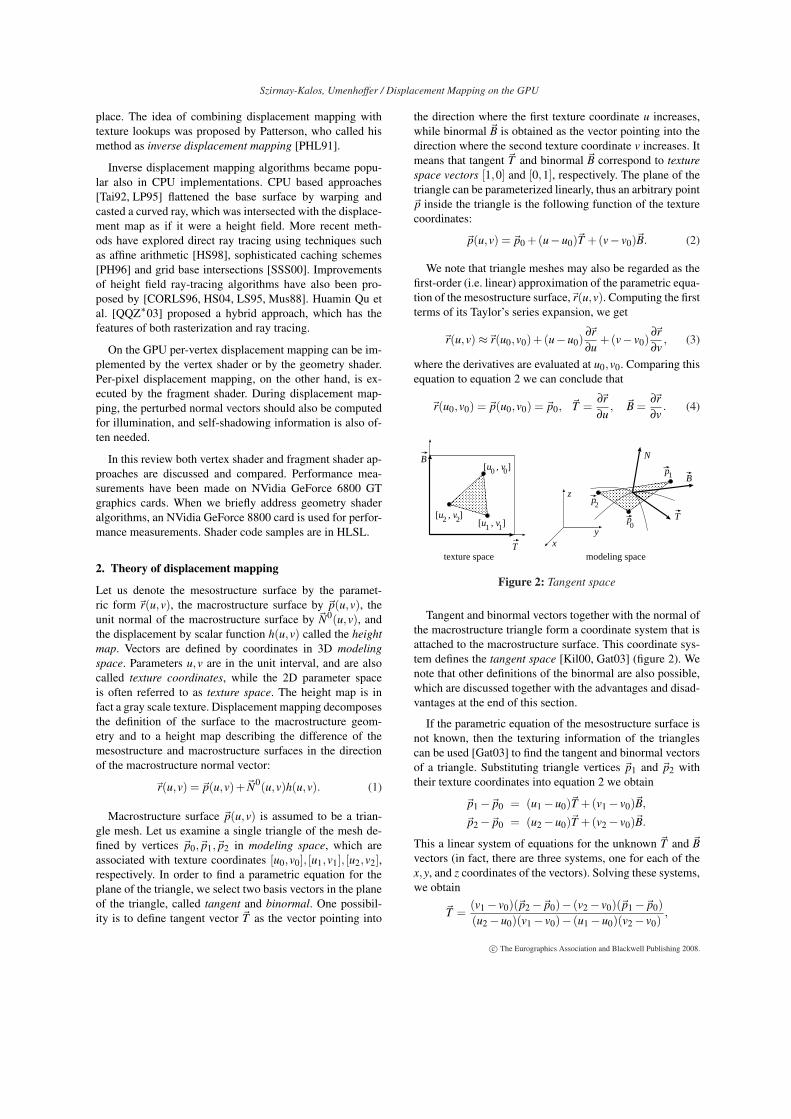
Macrostructure surface ~p(u,v) is assumed to be a trian-gle mesh. Let us examine a single triangle of the mesh de-fined by vertices ~p0,~p1,~p2 in modeling space, which areassociated with texture coordinates [u0,v0], [u1,v1], [u2,v2],respectively. In order to find a parametric equation for theplane of the triangle, we select two basis vectors in the planeof the triangle, called tangent and binormal. One possibil-ity is to define tangent vector ~T as the vector pointing into
the direction where the first texture coordinate u increases,while binormal ~B is obtained as the vector pointing into thedirection where the second texture coordinate v increases. Itmeans that tangent ~T and binormal ~B correspond to texturespace vectors [1,0] and [0,1], respectively. The plane of thetriangle can be parameterized linearly, thus an arbitrary point~p inside the triangle is the following function of the texturecoordinates:
~p(u,v) = ~p0 +(u−u0)~T +(v− v0)~B. (2)
We note that triangle meshes may also be regarded as thefirst-order (i.e. linear) approximation of the parametric equa-tion of the mesostructure surface,~r(u,v). Computing the firstterms of its Taylor’s series expansion, we get
~r(u,v)≈~r(u0,v0)+(u−u0)∂~r∂u
+(v− v0)∂~r∂v
, (3)
where the derivatives are evaluated at u0,v0. Comparing thisequation to equation 2 we can conclude that
~r(u0,v0) = ~p(u0,v0) = ~p0, ~T =∂~r∂u
, ~B =∂~r∂v
. (4)
T
B
T
B
N
xy
z
[u , v ]00
[u , v ]11
[u , v ]22 p
p
p
1
0
2
texture space modeling space
Figure 2: Tangent space
Tangent and binormal vectors together with the normal ofthe macrostructure triangle form a coordinate system that isattached to the macrostructure surface. This coordinate sys-tem defines the tangent space [Kil00, Gat03] (figure 2). Wenote that other definitions of the binormal are also possible,which are discussed together with the advantages and disad-vantages at the end of this section.
If the parametric equation of the mesostructure surface isnot known, then the texturing information of the trianglescan be used [Gat03] to find the tangent and binormal vectorsof a triangle. Substituting triangle vertices ~p1 and ~p2 withtheir texture coordinates into equation 2 we obtain
~p1−~p0 = (u1−u0)~T +(v1− v0)~B,
~p2−~p0 = (u2−u0)~T +(v2− v0)~B.
This a linear system of equations for the unknown ~T and ~Bvectors (in fact, there are three systems, one for each of thex,y, and z coordinates of the vectors). Solving these systems,we obtain
~T =(v1− v0)(~p2−~p0)− (v2− v0)(~p1−~p0)(u2−u0)(v1− v0)− (u1−u0)(v2− v0)
,
c© The Eurographics Association and Blackwell Publishing 2008.

Szirmay-Kalos, Umenhoffer / Displacement Mapping on the GPU
~B =(u1−u0)(~p2−~p0)− (u2−u0)(~p1−~p0)(u1−u0)(v2− v0)− (u2−u0)(v1− v0)
. (5)
The normal vector of the triangle can be obtained as thecross product of these vectors:
~N = ~T ×~B.
We often use the unit length normal vector ~N0 = ~N/|~N|instead of ~N. Then the surface is displaced by ~N0h. How-ever, there is a problem. Suppose that the object is scaleduniformly by a factor s. In this case we expect bumps alsoto grow similarly, but ~N0h remains constant. Neither wouldthe elimination of the normalization work, since if the dis-placement were defined as ~Nh = (~T ×~B)h, then scaling by swould multiply the displacement distances by s2. In order toavoid this, we can set the normal vector that is multiplied bythe height value as [Bli78]
~N =~T ×~B√
(|~T |2 + |~B|2)/2. (6)
The selection between alternative ~N0h and equation 6 ismore a modeling than a rendering issue. If we use unit nor-mals, then the displacement is independent of the size of thetriangle, and also of the scaling of the object. This makesthe design of the bumps easy and the scaling problem can besolved by scaling the height function generally for the ob-ject. Using equation 6, on the other hand, the bumps will behigher on triangles being large in modeling space but beingsmall in texture space. This makes the design of the heightmap more difficult. However, if we use a good parametriza-tion, where the texture to model space transformation haveroughly the same area expansion everywhere, then this prob-lem is eliminated. In this second case, uniform scaling wouldnot modify the appearence of the object, i.e. the relative sizesof the bumps.
In the remaining part of this paper we use the notation ~Nto refer to the normal vector used for displacement calcula-tion. This can be either the unit normal, or the normal scaledaccording to the length of the tangent and binormal vectors.
Note that in tangent space ~T ,~B,~N are orthonormal, thatis, they are orthogonal and have unit length. However, thesevectors are not necessarily orthonormal in modeling space(the transformation between the texture and modeling spacesis not always angle and distance preserving). We should beaware that the lengths of the tangent and binormal vectorsin modeling space are usually not 1, but express the expan-sion or shrinking of the texels as they are mapped onto thesurface. On the other hand, while the normal is orthogonalto both the tangent and the binormal, the tangent and the bi-normal vectors are not necessarily orthogonal. Of course inspecial cases, such as when a rectangle, sphere, cylinder, ro-tational surface, etc. are parameterized in the usual way, theorthogonality of these vectors is preserved, but this is not
true in the general case. Consider, for example, a shearedrectangle.
Having vectors ~T ,~B,~N in the modeling space and point~p0 corresponding to the origin of the tangent space, a point(u,v,h) in tangent space can be transformed to modelingspace as
~p(u,v) = ~p0 +[u,v,h] ·
~T~B~N
= ~p0 +[u,v,h] ·M,
where M is the transformation matrix from tangent space tomodeling space. This matrix is also called sometimes as TBNmatrix.
When transforming a vector ~d = ~p− ~p0, for examplethe view and light vectors, from modeling space to tangentspace, then the inverse of the matrix should be applied:
[u,v,h] = [dx,dy,dz] ·M−1.
To compute the inverse, in the general case we can ex-ploit only that the normal is orthogonal to the tangent andthe binormal:
u =(~T · ~d)~B2− (~B · ~d)(~B ·~T )
~B2~T 2− (~B ·~T )2,
v =(~B · ~d)~T 2− (~T · ~d)(~B ·~T )
~B2~T 2− (~B ·~T )2, h =
~N · ~d~N2
. (7)
If vectors ~T ,~B,~N are orthogonal to each other, then theseequations have simpler forms:
u =~T · ~d~T 2
, v =~B · ~d~B2
, h =~N · ~d~N2
.
If vectors ~T ,~B,~N were both orthogonal and had unit length,then the inverse of matrix M could be computed by simplytransposing the matrix. This is an important advantage, sotangent and binormal vectors are also often defined accord-ing to this requirement. Having obtained vectors ~T , ~B usingeither equation 4 or equation 5, and then ~N as their crossproduct, binormal ~B is recomputed as ~B = ~N×~T , and finallyall three vectors are normalized. The advantages of orthonor-mal ~T , ~B, ~N vectors are the easy transformation between tan-gent and modeling spaces, and the freedom of evaluating theillumination also in tangent space since the transformation totangent space is conformal i.e. angle preserving. Evaluatingthe illumination in tangent space is faster than in world spacesince light and view vectors change smoothly so they canbe transformed to tangent space per vertex, i.e. by the ver-tex shader, interpolated by the graphics hardware, and usedthe interpolated light and view vectors per fragment by thefragment shader. The disadvantage of the orthonormaliza-tion process is that we lose the intuitive interpretation that~T and ~B show the effects of increasing texture coordinates uand v, respectively, and we cannot imagine 3D tangent space
c© The Eurographics Association and Blackwell Publishing 2008.

Szirmay-Kalos, Umenhoffer / Displacement Mapping on the GPU
basis vectors as adding a third vector to the basis vectors ofthe 2D texture space.
When height function h(u,v) is stored as a texture, wehave to take into account that compact texture formats repre-sent values in the range of [0,1] with at most 8 bit fixed pointprecision, while the height function may have a higher rangeand may have even negative values. Thus the stored valuesshould be scaled and biased. Generally we use two con-stants SCALE and BIAS and convert the stored texel valueTexel(u,v) as
h(u,v) = BIAS +SCALE ·Texel(u,v). (8)
Height maps are often stored in the alpha channel of con-ventional color textures. Such representations are called re-lief textures [OB99, OBM00]. Relief textures and their ex-tensions are also used in image based rendering algorithms[Oli00, EY03, PS02].
Although this review deals with those displacement map-ping algorithms which store the height map in a two dimen-sional texture, we mention that three dimensional texturesalso received attention. Dietrich [Die00] introduced eleva-tion maps, converting the height field to a texture volume.This method can lead to visual artifacts at grazing angles,where the viewer can see through the spaces between theslices. Kautz and Seidel [KS01] extended Dietrich’s methodand minimized the errors at grazing angles. Lengyel used arendering technique to display fur interactively on arbitrarysurfaces [LPFH01].
2.1. Lighting displacement mapped surfaces
When mesostructure geometry ~r = ~p + ~N0h is shaded, itsreal normal vector should be inserted into the illuminationformulae. The mesostructure normal vector can be obtainedin modeling space as the cross product of two vectors in itstangent plane. These vectors can be the derivatives accord-ing to texture coordinates u,v [Bli78]. Using equation 1 weobtain
∂~r∂u
=∂~p∂u
+~N0 ∂h∂u
+∂~N0
∂uh≈ ~T +~N0 ∂h
∂u
since ∂~p/∂u = ~T and on a smooth macrostructure surface∂~N0/∂u ≈ 0. Similarly, the partial derivative according to vis
∂~r∂v
=∂~p∂v
+~N0 ∂h∂v
+∂~N0
∂vh≈ ~B+~N0 ∂h
∂v.
The mesostructure normal vector is the cross product ofthese derivatives:
~N′ = ∂~r∂u× ∂~r
∂v= ~N +(~N0×~B)
∂h∂u
+(~T ×~N0)∂h∂v
,
since ~T ×~B = ~N and ~N0×~N0 = 0.
In order to speed up the evaluation of the mesostructure
normal, vectors ~t = ~N0 × ~B and ~b = ~T × ~N0 can be pre-computed on the CPU and passed to the vertex shader if illu-mination is computed per vertex, or to the fragment shader ifillumination is computed per fragment. Since vectors~t and~bare in the tangent plane they can also play the roles of tangentand binormal vectors. Using these vectors the mesostructurenormal is
~N′ = ~N +~t∂h∂u
+~b∂h∂v
. (9)
The following fragment shader code computes themesostructure normal according to this formula, replacingthe derivatives by finite differences. The macrostructure nor-mal ~N, and tangent plane vectors~t,~b are passed in registersand are denoted by N, t, and b, respectively. The texture co-ordinates of the current point are in uv and the displacementis in the alpha channel of texture map hMap of resolutionWIDTH×HEIGHT.
float2 du=float2(1/WIDTH, 0);float2 dv=float2(0, 1/HEIGHT);float dhdu = SCALE/(2/WIDTH) *
(tex2D(hMap, uv+du).a -tex2D(hMap, uv-du).a);
float dhdv = SCALE/(2/HEIGHT) *(tex2D(hMap, uv+dv).a -tex2D(hMap, uv-dv).a);
// get model space normal vectorfloat3 mNormal = normalize(N+t*dhdu+b*dhdv);
On the other hand, instead of evaluating this formula toobtain mesostructure normals we can also use normal mapswhich store the mesostructure normals in textures. Heightvalues and normal vectors are usually organized in a waythat the r,g,b channels of a texel represent either the tangentspace or the modeling space normal vector, and the alphachannel the height value.
Storing modeling space normal vectors in normal mapshas the disadvantage that the normal map cannot be tiledonto curved surfaces since multiple tiles would associatethe same texel with several points on the surface, which donot necessarily have the same mesostructure normal. Notethat by storing tangent space normal vectors this problem issolved since in this case the mesostructure normal dependsnot only on the stored normal but also on the transformationbetween tangent and modeling spaces, which can follow theorientation change of curved faces.
Having the mesostructure normal, the next crucial prob-lem is to select the coordinate system where we evaluate theillumination formula, for example, the Phong-Blinn reflec-tion model [Bli77]. Light and view vectors are available inworld or in camera space, while the shading normal is usu-ally available in tangent space. The generally correct solu-tion is to transform the normal vector to world or cameraspace and evaluate the illumination there. However, if themappings between world space and modeling space, and be-tween modeling space and tangent space are angle preserv-
c© The Eurographics Association and Blackwell Publishing 2008.
Szirmay-Kalos, Umenhoffer / Displacement Mapping on the GPU
ing, then view and light vectors can also be transformed totangent space and we can compute the illumination formulahere.
2.2. Obtaining height and normal maps
Height fields are natural representations in a variety of con-texts, including e.g. water surface and terrain modeling.In these cases, height maps are provided by simulation ormeasurement processes. Height maps are gray scale im-ages and can thus also be generated by 2D drawing tools.They can be the results of surface simplification when thedifference of the detailed and the macrostructure surfaceis computed [CMSR98, Bla92, ATI03]. In this way heightand normal map construction is closely related to tessel-lation [GH99, DH00, DKS01, MM02, EBAB05] and subdi-vision algorithms [Cat74, BS05]. Using light measurementtools and assuming that the surface is diffuse, the mesostruc-ture of the surface can also be determined from reflectionpatterns using photometric stereo also called shape fromshading techniques [ZTCS99, RTG97, LKG∗03].
Displacement maps can also be the results of renderingduring impostor generation, when complex objects are ras-terized to textures, which are then displayed instead of theoriginal models [JWP05]. Copying not only the color chan-nels but also the depth buffer, the texture can be equippedwith displacement values [OBM00, MJW07].
The height map texture is a discrete representation of acontinuous function, thus can cause aliasing and samplingartifacts. Fournier [Fou92] pre-filtered height maps to avoidaliasing problems. Standard bi- and tri-linear interpolationof normal maps work well if the normal field is continu-ous, but may result in visible artifacts in the areas where thefield is discontinuous, which is common for surfaces withcreases and dents. Sophisticated filtering techniques basedon feature-based textures [WMF∗00, TC05, PRZ05] and sil-houette maps [Sen04] have been proposed in the more gen-eral context of texture mapping to overcome these problems.
3. Per-vertex displacement mapping on the GPU
Displacement mapping can be implemented either in the ver-tex shader modifying the vertices, or in the fragment shaderre-evaluating the visibility or modifying the texture coordi-nates. This section presents the vertex shader solution.
Graphics hardware up to Shader Model 3 (or Direct3D 9)is unable to change the topology of the triangle mesh, thusonly the original vertices can be perturbed. This has beenchanged in Shader Model 4 (i.e. Direct3D 10) compatiblehardware. Assuming Shader Model 3 GPUs the real modifi-cation of the surface geometry requires a highly tessellated,but smooth surface, which can be modulated by a height mapin the vertex shader program.
3.1. Vertex modification on the vertex shader
The vertices of the triangles are displaced in the directionof the normal of the macrostructure surface according to theheight map. New, mesostructure normal vectors are also as-signed to the displaced vertices to accurately simulate thesurface lighting. Since the introduction of Shader Model 3.0compatible hardware, the vertex shader is allowed to accessthe texture memory, thus the height map can be stored in atexture. In earlier, Shader Model 1 or 2 compatible hardwareonly procedural displacement mapping could be executed inthe vertex shader.
highly tessellated macrostructure surface
height map storedas a texture
vertexshader rasterization fragment
shader
modified vertices
Figure 3: Displacement mapping on the vertex shader
The following vertex shader program takes modelingspace point Position with macrostructure normal vec-tor Normal and texture coordinates uv, reads height maphMap, computes modeling space vertex position mPos, andtransforms the modified point to clipping space hPos:
float h = tex2Dlod(hMap, uv).a * SCALE + BIAS;float3 mPos = Position + Normal * h;hPos = mul(float4(mPos,1), WorldViewProj);
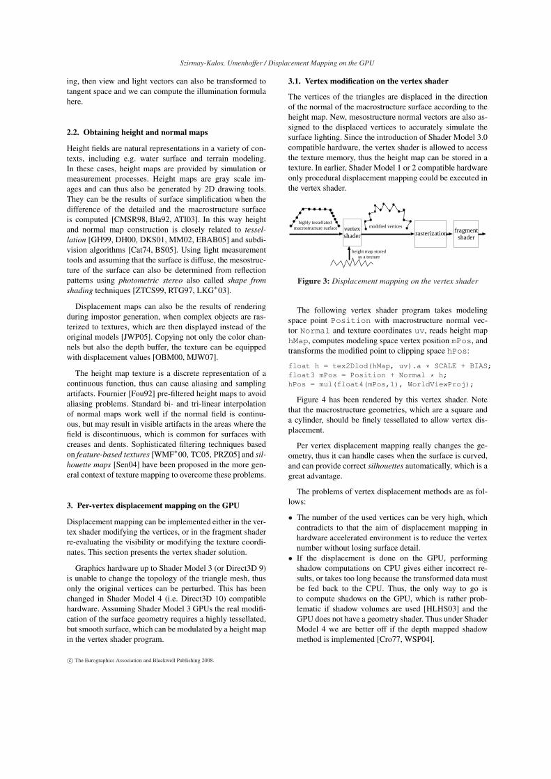
Figure 4 has been rendered by this vertex shader. Notethat the macrostructure geometries, which are a square anda cylinder, should be finely tessellated to allow vertex dis-placement.
Per vertex displacement mapping really changes the ge-ometry, thus it can handle cases when the surface is curved,and can provide correct silhouettes automatically, which is agreat advantage.
The problems of vertex displacement methods are as fol-lows:
• The number of the used vertices can be very high, whichcontradicts to that the aim of displacement mapping inhardware accelerated environment is to reduce the vertexnumber without losing surface detail.
• If the displacement is done on the GPU, performingshadow computations on CPU gives either incorrect re-sults, or takes too long because the transformed data mustbe fed back to the CPU. Thus, the only way to go isto compute shadows on the GPU, which is rather prob-lematic if shadow volumes are used [HLHS03] and theGPU does not have a geometry shader. Thus under ShaderModel 4 we are better off if the depth mapped shadowmethod is implemented [Cro77, WSP04].
c© The Eurographics Association and Blackwell Publishing 2008.
Szirmay-Kalos, Umenhoffer / Displacement Mapping on the GPU
BIAS = 0 BIAS = 0SCALE = 0.24 SCALE = 0.30
FPS = 620 FPS = 520
Figure 4: Vertex displacement with shading (top row). Thegeometry should be finely tesselated (bottom row).
• GPUs have usually more pixel-processing power thanvertex-processing power, but the unified shader architec-ture [Sco07] can find a good balance.
• Pixel shaders are better equipped to access textures. OlderGPUs do not allow texture access within a vertex shader.More recent GPUs do, but the access modes are limited,and the texture access in the vertex shader is slower thanin the fragment shader.
• The vertex shader always executes once for each vertex inthe model, but the fragment shader executes only once perpixel on the screen. This means that in fragment shadersthe work is concentrated on nearby objects where it isneeded the most, but vertex shader solutions devote thesame effort to all parts of the geometry, even to invisibleor hardly visible parts.
3.2. Shader Model 4 outlook
Shader Model 4 has introduced a new stage in the renderingpipeline between the vertex shader and the rasterizer unit,called the geometry shader [Bly06]. The geometry shaderprocesses primitives and can create new vertices, thus itseems to be an ideal tessellator. So it becomes possible toimplement displacement mapping in a way that the vertexshader transforms the macrostructure surface, the geometryshader tessellates and modulates it with the height map togenerate the mesostructure mesh, which is output to the ras-terizer unit.
Though subdividing the meshes with the geometry shaderlooks a good choice, care should be taken to implement thisidea. The number of new triangles generated by the geom-etry shader is limited by the maximum output size, whichis currently 1024× 32 = 32768 bits. This limitation can beovercome if the data is fed back to the geometry shader againcreating levels of subdivisions. One should take into accountthat subdividing a triangle into hundreds of triangles maygive good quality results but highly reduces performance.The number of new triangles should depend on the frequencyof the height map, and more vertices should be inserted intoareas where the height map has high variation and less de-tailed tessellation is needed where the height map changessmoothly. The texture and model space areas of the trianglesshould also influence the number of subdivisions. The subdi-vision algorithm should also consider the orientation of thetriangles according to the viewer as triangles perpendicularto the view ray may not require as many subdivisions, whilefaces seen at grazing angles, and especially silhouette edgesshould be subdivided into more pieces.
Developing geometry shader programs that meet all therequirements described above is not easy, and it will be animportant research area in the near future.
4. Per-pixel displacement mapping on the GPU
macrostructure surface
height map storedas a texture
vertexshader rasterization
fragmentshader
visibilityray
processedpoint
modifiedvisible point
pixel
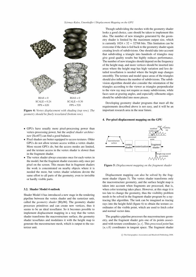
Figure 5: Displacement mapping on the fragment shader
Displacement mapping can also be solved by the frag-ment shader (figure 5). The vertex shader transforms onlythe macrostructure geometry, and the surface height map istaken into account when fragments are processed, that is,when color texturing takes place. However, at this stage it istoo late to change the geometry, thus the visibility problemneeds to be solved in the fragment shader program by a ray-tracing like algorithm. The task can be imagined as tracingrays into the height field (figure 6) to obtain the texture co-ordinates of the visible point, which are used to fetch colorand normal vector data.
The graphics pipeline processes the macrostructure geom-etry, and the fragment shader gets one of its points associ-ated with texture coordinates [u,v]. This processed point has(u,v,0) coordinates in tangent space. The fragment shader
c© The Eurographics Association and Blackwell Publishing 2008.
Szirmay-Kalos, Umenhoffer / Displacement Mapping on the GPU
(u,v,0)
N
T, B
h
(u’,v’, h(u’,v’))
macrostructure surface
pixel
processed point
visible point
(u’,v’)
V
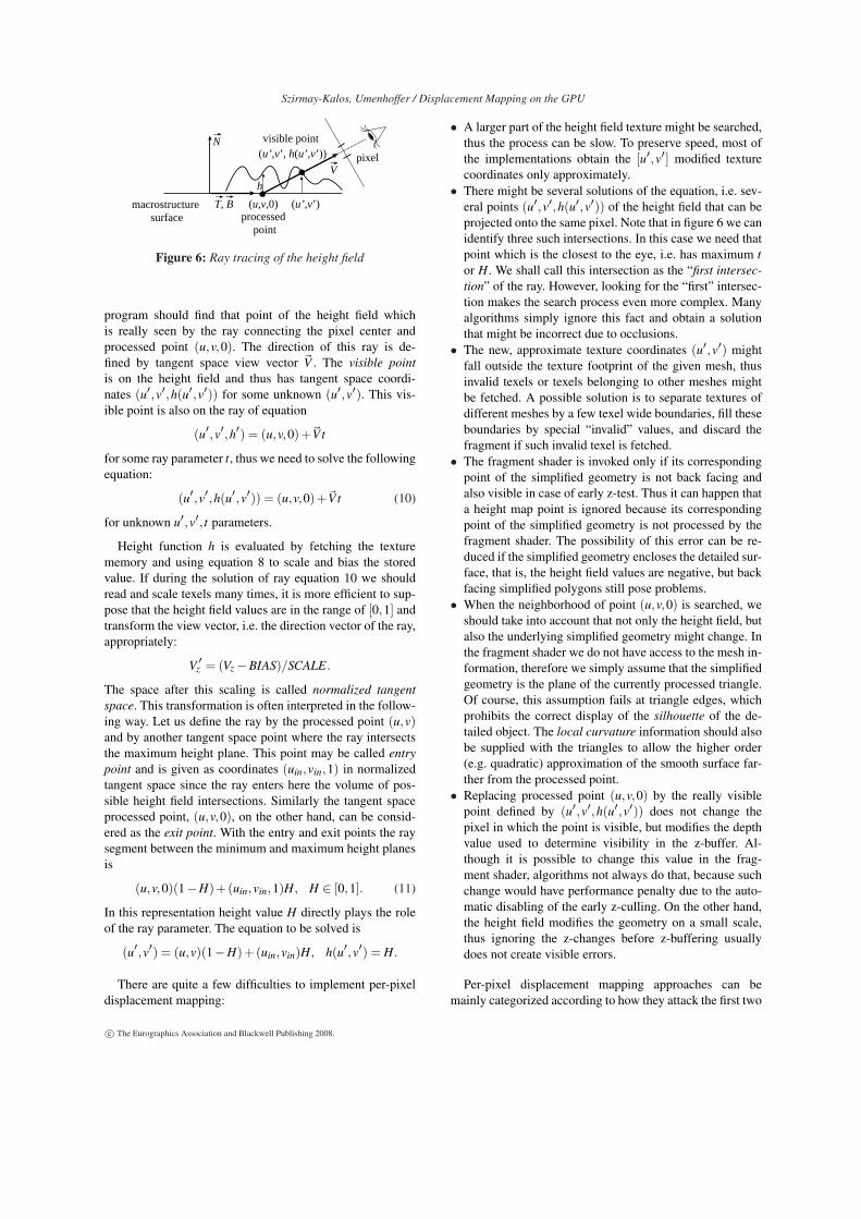
Figure 6: Ray tracing of the height field
program should find that point of the height field whichis really seen by the ray connecting the pixel center andprocessed point (u,v,0). The direction of this ray is de-fined by tangent space view vector ~V . The visible pointis on the height field and thus has tangent space coordi-nates (u′,v′,h(u′,v′)) for some unknown (u′,v′). This vis-ible point is also on the ray of equation
(u′,v′,h′) = (u,v,0)+~Vt
for some ray parameter t, thus we need to solve the followingequation:
(u′,v′,h(u′,v′)) = (u,v,0)+~Vt (10)
for unknown u′,v′, t parameters.
Height function h is evaluated by fetching the texturememory and using equation 8 to scale and bias the storedvalue. If during the solution of ray equation 10 we shouldread and scale texels many times, it is more efficient to sup-pose that the height field values are in the range of [0,1] andtransform the view vector, i.e. the direction vector of the ray,appropriately:
V ′z = (Vz−BIAS)/SCALE.
The space after this scaling is called normalized tangentspace. This transformation is often interpreted in the follow-ing way. Let us define the ray by the processed point (u,v)and by another tangent space point where the ray intersectsthe maximum height plane. This point may be called entrypoint and is given as coordinates (uin,vin,1) in normalizedtangent space since the ray enters here the volume of pos-sible height field intersections. Similarly the tangent spaceprocessed point, (u,v,0), on the other hand, can be consid-ered as the exit point. With the entry and exit points the raysegment between the minimum and maximum height planesis
(u,v,0)(1−H)+(uin,vin,1)H, H ∈ [0,1]. (11)
In this representation height value H directly plays the roleof the ray parameter. The equation to be solved is
(u′,v′) = (u,v)(1−H)+(uin,vin)H, h(u′,v′) = H.
There are quite a few difficulties to implement per-pixeldisplacement mapping:
• A larger part of the height field texture might be searched,thus the process can be slow. To preserve speed, most ofthe implementations obtain the [u′,v′] modified texturecoordinates only approximately.
• There might be several solutions of the equation, i.e. sev-eral points (u′,v′,h(u′,v′)) of the height field that can beprojected onto the same pixel. Note that in figure 6 we canidentify three such intersections. In this case we need thatpoint which is the closest to the eye, i.e. has maximum tor H. We shall call this intersection as the “first intersec-tion” of the ray. However, looking for the “first” intersec-tion makes the search process even more complex. Manyalgorithms simply ignore this fact and obtain a solutionthat might be incorrect due to occlusions.
• The new, approximate texture coordinates (u′,v′) mightfall outside the texture footprint of the given mesh, thusinvalid texels or texels belonging to other meshes mightbe fetched. A possible solution is to separate textures ofdifferent meshes by a few texel wide boundaries, fill theseboundaries by special “invalid” values, and discard thefragment if such invalid texel is fetched.
• The fragment shader is invoked only if its correspondingpoint of the simplified geometry is not back facing andalso visible in case of early z-test. Thus it can happen thata height map point is ignored because its correspondingpoint of the simplified geometry is not processed by thefragment shader. The possibility of this error can be re-duced if the simplified geometry encloses the detailed sur-face, that is, the height field values are negative, but backfacing simplified polygons still pose problems.
• When the neighborhood of point (u,v,0) is searched, weshould take into account that not only the height field, butalso the underlying simplified geometry might change. Inthe fragment shader we do not have access to the mesh in-formation, therefore we simply assume that the simplifiedgeometry is the plane of the currently processed triangle.Of course, this assumption fails at triangle edges, whichprohibits the correct display of the silhouette of the de-tailed object. The local curvature information should alsobe supplied with the triangles to allow the higher order(e.g. quadratic) approximation of the smooth surface far-ther from the processed point.
• Replacing processed point (u,v,0) by the really visiblepoint defined by (u′,v′,h(u′,v′)) does not change thepixel in which the point is visible, but modifies the depthvalue used to determine visibility in the z-buffer. Al-though it is possible to change this value in the frag-ment shader, algorithms not always do that, because suchchange would have performance penalty due to the auto-matic disabling of the early z-culling. On the other hand,the height field modifies the geometry on a small scale,thus ignoring the z-changes before z-buffering usuallydoes not create visible errors.
Per-pixel displacement mapping approaches can bemainly categorized according to how they attack the first two
c© The Eurographics Association and Blackwell Publishing 2008.

Szirmay-Kalos, Umenhoffer / Displacement Mapping on the GPU
challenges of this list, that is, whether or not they aim at ac-curate intersection calculation and at always finding the firstintersection.
Non-iterative or single-step methods correct the texturecoordinates using just local information, thus they need onlyat most one extra texture access but may provide bad results.
Iterative methods explore the height field globally thusthey can potentially find the exact intersection point but theyread the texture memory many times for each fragment. Iter-ative techniques can be further classified to safe methods thattry to guarantee that the first intersection is found, and to un-safe methods that may result in the second, third, etc. inter-section point if the ray intersects the height field many times.Since unsafe methods are much faster than safe methods itmakes sense to combine the two approaches. In combinedmethods first a safe iterative method reduces the search spaceto an interval where only one intersection exists, then an un-safe method computes the accurate intersection quickly.
In the following subsections we review different fragmentshader implementations of the height field rendering.
4.1. Non-iterative methods
Non-iterative methods read the height map at the processedpoint and using this local information obtain more accuratetexture coordinates, which will address the normal map andcolor textures.
4.1.1. Bump mapping
normalnormal
viewlight
N
T, B
h
macrostructure surface
macrostructure surface
Figure 7: Bump mapping
Bump mapping [Bli78] can be seen as a strongly sim-plified version of displacement mapping (figure 7). We in-cluded bump mapping into this survey for the sake of com-pleteness and to allow comparisons. If the uneven surfacehas very small bumps it can be estimated as being totallyflat. In case of flat surfaces the approximated visible point(u′,v′,h(u′,v′)) is equal to the processed point (u,v,0).However, in order to visualize bumps, it is necessary to sim-ulate how light affects them. The simplest way is to read themesostructure normal vectors from a normal map and usethese normals to perform lighting.
This technique was implemented in hardwareeven before the emergence of programmable GPUs[PAC97, Kil00, BERW97, TCRS00]. A particularly popular
FPS = 695 FPS = 690
Figure 8: Texture mapping (left) and texture mapping withbump mapping (right).
simplification used a simple embossing trick to simulatebump mapping for diffuse surfaces [Bli78, Sch94]. Beckerand Max extended bump mapping to account for occlusions[BM93], and called their technique redistribution bump-mapping. They also described how to switch between threerendering techniques (BRDF, redistribution bump-mappingand displacement mapping) within a single object accordingto the amount of visible surface detail.
4.1.2. Parallax mapping
Taking into account the height at the processed point par-allax mapping [KKI∗01] not only controls the shading nor-mals as bump mapping, but also modifies the texture coordi-nates used to obtain mesostructure normals and color data.
(u,v)
N
T, B
h
(u’,v’)macrostructuresurface
constant height surface
V
Figure 9: Parallax mapping
The texture coordinates are modified assuming that theheight field is constant h(u,v) everywhere in the neighbor-hood of (u,v). As can be seen in figure 9, the original (u,v)texture coordinates get substituted by (u′,v′), which arecalculated from the direction of tangent space view vector~V = (Vx,Vy,Vz) and height value h(u,v) read from a textureat point (u,v). The assumption on a constant height surface
c© The Eurographics Association and Blackwell Publishing 2008.
Szirmay-Kalos, Umenhoffer / Displacement Mapping on the GPU
simplifies the ray equation to
(u′,v′,h(u,v)) = (u,v,0)+~Vt,
which has the following solution:
(u′,v′) = (u,v)+h(u,v)(
Vx
Vz,Vy
Vz
).
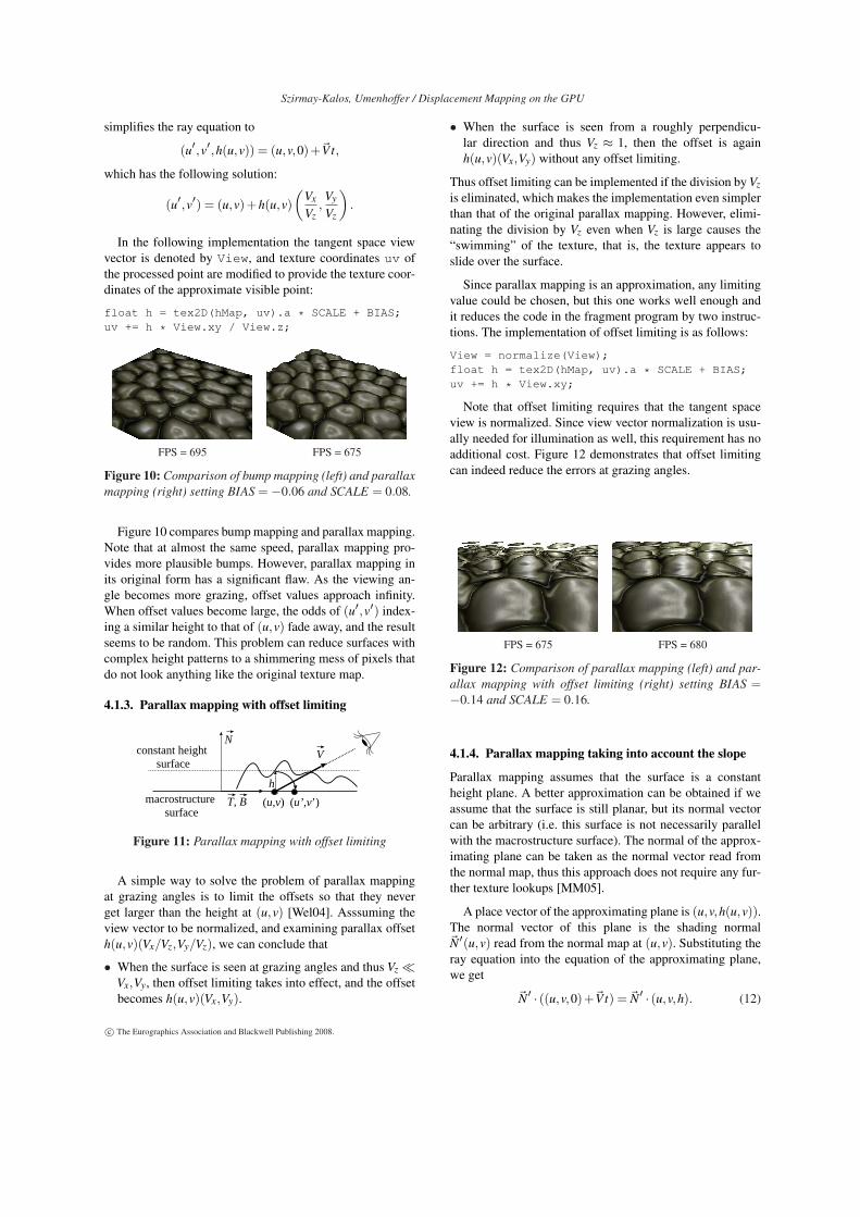
In the following implementation the tangent space viewvector is denoted by View, and texture coordinates uv ofthe processed point are modified to provide the texture coor-dinates of the approximate visible point:
float h = tex2D(hMap, uv).a * SCALE + BIAS;uv += h * View.xy / View.z;
FPS = 695 FPS = 675
Figure 10: Comparison of bump mapping (left) and parallaxmapping (right) setting BIAS =−0.06 and SCALE = 0.08.
Figure 10 compares bump mapping and parallax mapping.Note that at almost the same speed, parallax mapping pro-vides more plausible bumps. However, parallax mapping inits original form has a significant flaw. As the viewing an-gle becomes more grazing, offset values approach infinity.When offset values become large, the odds of (u′,v′) index-ing a similar height to that of (u,v) fade away, and the resultseems to be random. This problem can reduce surfaces withcomplex height patterns to a shimmering mess of pixels thatdo not look anything like the original texture map.
4.1.3. Parallax mapping with offset limiting
(u,v)
N
T, B
h
(u’,v’)macrostructure surface
constant height surface
V
Figure 11: Parallax mapping with offset limiting
A simple way to solve the problem of parallax mappingat grazing angles is to limit the offsets so that they neverget larger than the height at (u,v) [Wel04]. Asssuming theview vector to be normalized, and examining parallax offseth(u,v)(Vx/Vz,Vy/Vz), we can conclude that
• When the surface is seen at grazing angles and thus Vz ¿Vx,Vy, then offset limiting takes into effect, and the offsetbecomes h(u,v)(Vx,Vy).
• When the surface is seen from a roughly perpendicu-lar direction and thus Vz ≈ 1, then the offset is againh(u,v)(Vx,Vy) without any offset limiting.
Thus offset limiting can be implemented if the division by Vzis eliminated, which makes the implementation even simplerthan that of the original parallax mapping. However, elimi-nating the division by Vz even when Vz is large causes the“swimming” of the texture, that is, the texture appears toslide over the surface.
Since parallax mapping is an approximation, any limitingvalue could be chosen, but this one works well enough andit reduces the code in the fragment program by two instruc-tions. The implementation of offset limiting is as follows:
View = normalize(View);float h = tex2D(hMap, uv).a * SCALE + BIAS;uv += h * View.xy;
Note that offset limiting requires that the tangent spaceview is normalized. Since view vector normalization is usu-ally needed for illumination as well, this requirement has noadditional cost. Figure 12 demonstrates that offset limitingcan indeed reduce the errors at grazing angles.
FPS = 675 FPS = 680
Figure 12: Comparison of parallax mapping (left) and par-allax mapping with offset limiting (right) setting BIAS =−0.14 and SCALE = 0.16.
4.1.4. Parallax mapping taking into account the slope
Parallax mapping assumes that the surface is a constantheight plane. A better approximation can be obtained if weassume that the surface is still planar, but its normal vectorcan be arbitrary (i.e. this surface is not necessarily parallelwith the macrostructure surface). The normal of the approx-imating plane can be taken as the normal vector read fromthe normal map, thus this approach does not require any fur-ther texture lookups [MM05].
A place vector of the approximating plane is (u,v,h(u,v)).The normal vector of this plane is the shading normal~N′(u,v) read from the normal map at (u,v). Substituting theray equation into the equation of the approximating plane,we get
~N′ · ((u,v,0)+~Vt) = ~N′ · (u,v,h). (12)
c© The Eurographics Association and Blackwell Publishing 2008.
Szirmay-Kalos, Umenhoffer / Displacement Mapping on the GPU
(u,v)
N
T, B
h
(u’,v’)macrostructure surface
N’
V
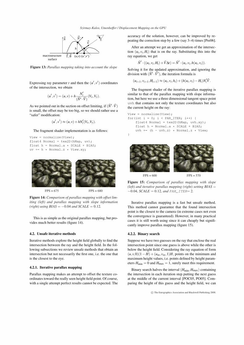
Figure 13: Parallax mapping taking into account the slope
Expressing ray parameter t and then the (u′,v′) coordinatesof the intersection, we obtain
(u′,v′) = (u,v)+hN′z
(~N′ ·~V )(Vx,Vy).
As we pointed out in the section on offset limiting, if (~N′ ·~V )is small, the offset may be too big, so we should rather use a“safer” modification:
(u′,v′)≈ (u,v)+hN′z(Vx,Vy).
The fragment shader implementation is as follows:
View = normalize(View);float4 Normal = tex2D(hMap, uv);float h = Normal.a * SCALE + BIAS;uv += h * Normal.z * View.xy;
FPS = 675 FPS = 680
Figure 14: Comparison of parallax mapping with offset lim-iting (left) and parallax mapping with slope information(right) using BIAS =−0.04 and SCALE = 0.12.
This is as simple as the original parallax mapping, but pro-vides much better results (figure 14).
4.2. Unsafe iterative methods
Iterative methods explore the height field globally to find theintersection between the ray and the height field. In the fol-lowing subsections we review unsafe methods that obtain anintersection but not necessarily the first one, i.e. the one thatis the closest to the eye.
4.2.1. Iterative parallax mapping
Parallax mapping makes an attempt to offset the texture co-ordinates toward the really seen height field point. Of course,with a single attempt perfect results cannot be expected. The
accuracy of the solution, however, can be improved by re-peating the correction step by a few (say 3–4) times [Pre06].
After an attempt we get an approximation of the intersec-tion (ui,vi,Hi) that is on the ray. Substituting this into theray equation, we get
~N′ · ((ui,vi,Hi)+~V ∆t) = ~N′ · (ui,vi,h(ui,vi)).
Solving it for the updated approximation, and ignoring thedivision with (~N′ ·~V ′), the iteration formula is
(ui+1,vi+1,Hi+1)≈ (ui,vi,hi)+(h(ui,vi)−Hi)N′z~V .
The fragment shader of the iterative parallax mapping issimilar to that of the parallax mapping with slope informa-tion, but here we use a three dimensional tangent space pointuvh that contains not only the texture coordinates but alsothe current height on the ray:
View = normalize(View);for(int i = 0; i < PAR_ITER; i++) {
float4 Normal = tex2D(hMap, uvh.xy);float h = Normal.a * SCALE + BIAS;uvh += (h - uvh.z) * Normal.z * View;
}
FPS = 600 FPS = 570
Figure 15: Comparison of parallax mapping with slope(left) and iterative parallax mapping (right) setting BIAS =−0.04, SCALE = 0.12, and PAR_ITER= 2.
Iterative parallax mapping is a fast but unsafe method.This method cannot guarantee that the found intersectionpoint is the closest to the camera (in extreme cases not eventhe convergence is guaranteed). However, in many practicalcases it is still worth using since it can cheaply but signifi-cantly improve parallax mapping (figure 15).
4.2.2. Binary search
Suppose we have two guesses on the ray that enclose the realintersection point since one guess is above while the other isbelow the height field. Considering the ray equation of form(u,v,0)(1−H)+ (uin,vin,1)H, points on the minimum andmaximum height values, i.e. points defined by height param-eters Hmin = 0 and Hmax = 1, surely meet this requirement.
Binary search halves the interval (Hmin,Hmax) containingthe intersection in each iteration step putting the next guessat the middle of the current interval [POC05, PO05]. Com-paring the height of this guess and the height field, we can
c© The Eurographics Association and Blackwell Publishing 2008.

Szirmay-Kalos, Umenhoffer / Displacement Mapping on the GPU
(u’,v’)
N
T, B
31
24
V5
Figure 16: Binary search that stops at point 5
decide whether or not the middle point is below the surface.Then we keep that half interval where one endpoint is abovewhile the other is below the height field.
In the following implementation the texture coordinates atthe entry and exit points are denoted by uvin and uvout,respectively, and the height values at the two endpoints ofthe current interval are Hmin and Hmax.
float2 uv; // texture coords of intersectionfor (int i = 0; i < BIN_ITER; i++) {
H = (Hmin + Hmax)/2; // middleuv = uvin * H + uvout * (1-H);float h = tex2D(hMap, uv).a;if (H <= h) Hmin = H; // belowelse Hmax = H; // above
}
Figure 17: Binary search using 5 iteration steps. The ren-dering speed is 455 FPS.
The binary search procedure quickly converges to an in-tersection but may not result in the first intersection that hasthe maximum height value (figure 17).
4.2.3. Secant method
Binary search simply halves the interval potentially contain-ing the intersection point without taking into account theunderlying geometry. The secant method [YJ04, RSP06] onthe other hand, assumes that the surface is planar betweenthe two guesses and computes the intersection between theplanar surface and the ray. It means that if the surface werereally a plane between the first two candidate points, thisintersection point could be obtained at once. The heightfield is checked at the intersection point and one endpointof the current interval is replaced keeping always a pair of
end points where one end is above while the other is be-low the height field. As has been pointed out in [SKALP05]the name “secant” is not precise from mathematical point ofview since the secant method in mathematics always keepsthe last two guesses and does not care of having a pair ofpoints that enclose the intersection. Mathematically the rootfinding scheme used in displacement mapping is equivalentto the false position method. We note that it would be worthchecking the real secant algorithm as well, which almost al-ways converges faster than the false position method, but un-fortunately, its convergence is not guaranteed in all cases.
(u,v)
N
T, B
∆
(u’,v’)macrostructure surface
∆a bH
V
aHb
Figure 18: The secant method
To discuss the implementation of the secant method, letus consider the last two points of the linear search, point~b that is below the height field, and ~a that is the last pointwhich is above the height field. Points~b and~a are associatedwith height parameters Hb and Ha, respectively. The leveldifferences between the points on the ray and the height fieldat ~a and~b are denoted by ∆a and ∆b, respectively (note that∆a ≥ 0 and ∆b < 0 hold). Figure 18 depicts these points inthe plane containing viewing vector~V . We wish to obtain theintersection point of the view ray and of the line between thepoints on the height field just above ~a and below~b.
Using figure 18 and the simple similarity, the ray parame-ter of the intersection point is
Hnew = Hb +(Ha−Hb)∆a
∆a−∆b.
Note that we should use ∆b with negative sign since ∆bmeans a signed distance and it is negative.
Checking the height here again, the new point may be ei-ther above or below the height field. Replacing the previouspoint of the same type with the new point, the same proce-dure can be repeated iteratively.
The secant algorithm is as follows:
for (int i = 0; i < SEC_ITER; i++) {H = Hb + (Ha-Hb) /(Da-Db) * Da;float2 uv = uvin * H + uvout * (1-H);D = H - tex2D(hMap, uv).a ;if (D < 0) {
Db = D; Hb = H;} else {
Da = D; Ha = H;}
}
c© The Eurographics Association and Blackwell Publishing 2008.
Szirmay-Kalos, Umenhoffer / Displacement Mapping on the GPU
4.3. Safe iterative methods
Safe methods pay attention to finding the first intersectioneven if the ray intersects the height field several times. Thefirst algorithm of this section, called linear search is only“quasi-safe”. If the steps are larger than the texel size, thisalgorithm may still fail, but its probability is low. Other tech-niques, such as the dilation-erosion map, the sphere, cone,and pyramidal mapping are safe, but require preprocessingthat generates data encoding the empty spaces in the heightfield. Note that safe methods guarantee that they do not skipthe first intersection, but cannot guarantee that the intersec-tion is precisely located if the number of iterations is limited.
4.3.1. Linear search
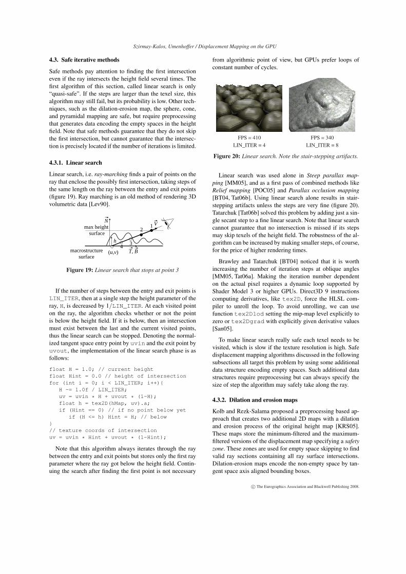
Linear search, i.e. ray-marching finds a pair of points on theray that enclose the possibly first intersection, taking steps ofthe same length on the ray between the entry and exit points(figure 19). Ray marching is an old method of rendering 3Dvolumetric data [Lev90].
(u,v)
N
T, B
h
macrostructuresurface
max height surface
12
3
V
4
Figure 19: Linear search that stops at point 3
If the number of steps between the entry and exit points isLIN_ITER, then at a single step the height parameter of theray, H, is decreased by 1/LIN_ITER. At each visited pointon the ray, the algorithm checks whether or not the pointis below the height field. If it is below, then an intersectionmust exist between the last and the current visited points,thus the linear search can be stopped. Denoting the normal-ized tangent space entry point by uvin and the exit point byuvout, the implementation of the linear search phase is asfollows:
float H = 1.0; // current heightfloat Hint = 0.0 // height of intersectionfor (int i = 0; i < LIN_ITER; i++){
H -= 1.0f / LIN_ITER;uv = uvin * H + uvout * (1-H);float h = tex2D(hMap, uv).a;if (Hint == 0) // if no point below yet
if (H <= h) Hint = H; // below}// texture coords of intersectionuv = uvin * Hint + uvout * (1-Hint);
Note that this algorithm always iterates through the raybetween the entry and exit points but stores only the first rayparameter where the ray got below the height field. Contin-uing the search after finding the first point is not necessary
from algorithmic point of view, but GPUs prefer loops ofconstant number of cycles.
FPS = 410 FPS = 340LIN_ITER = 4 LIN_ITER = 8
Figure 20: Linear search. Note the stair-stepping artifacts.
Linear search was used alone in Steep parallax map-ping [MM05], and as a first pass of combined methods likeRelief mapping [POC05] and Parallax occlusion mapping[BT04, Tat06b]. Using linear search alone results in stair-stepping artifacts unless the steps are very fine (figure 20).Tatarchuk [Tat06b] solved this problem by adding just a sin-gle secant step to a fine linear search. Note that linear searchcannot guarantee that no intersection is missed if its stepsmay skip texels of the height field. The robustness of the al-gorithm can be increased by making smaller steps, of course,for the price of higher rendering times.
Brawley and Tatarchuk [BT04] noticed that it is worthincreasing the number of iteration steps at oblique angles[MM05, Tat06a]. Making the iteration number dependenton the actual pixel requires a dynamic loop supported byShader Model 3 or higher GPUs. Direct3D 9 instructionscomputing derivatives, like tex2D, force the HLSL com-piler to unroll the loop. To avoid unrolling, we can usefunction tex2Dlod setting the mip-map level explicitly tozero or tex2Dgrad with explicitly given derivative values[San05].
To make linear search really safe each texel needs to bevisited, which is slow if the texture resolution is high. Safedisplacement mapping algorithms discussed in the followingsubsections all target this problem by using some additionaldata structure encoding empty spaces. Such additional datastructures require preprocessing but can always specify thesize of step the algorithm may safely take along the ray.
4.3.2. Dilation and erosion maps
Kolb and Rezk-Salama proposed a preprocessing based ap-proach that creates two additional 2D maps with a dilationand erosion process of the original height map [KRS05].These maps store the minimum-filtered and the maximum-filtered versions of the displacement map specifying a safetyzone. These zones are used for empty space skipping to findvalid ray sections containing all ray surface intersections.Dilation-erosion maps encode the non-empty space by tan-gent space axis aligned bounding boxes.
c© The Eurographics Association and Blackwell Publishing 2008.
Szirmay-Kalos, Umenhoffer / Displacement Mapping on the GPU
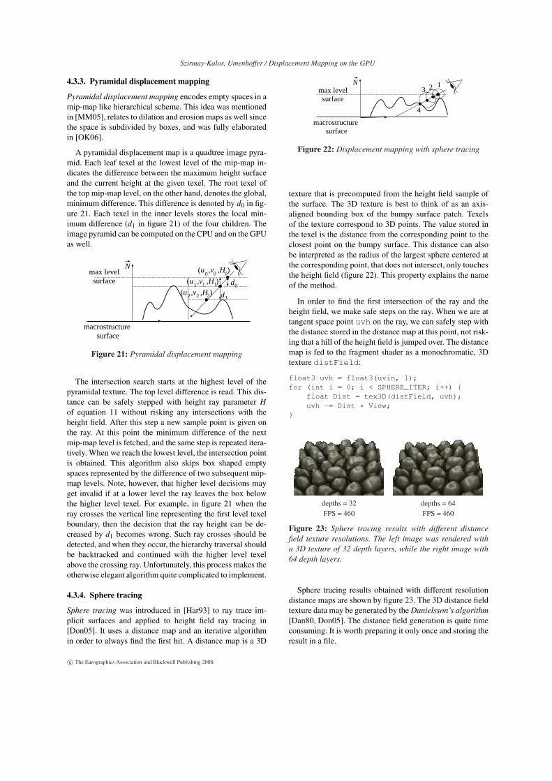
4.3.3. Pyramidal displacement mapping
Pyramidal displacement mapping encodes empty spaces in amip-map like hierarchical scheme. This idea was mentionedin [MM05], relates to dilation and erosion maps as well sincethe space is subdivided by boxes, and was fully elaboratedin [OK06].
A pyramidal displacement map is a quadtree image pyra-mid. Each leaf texel at the lowest level of the mip-map in-dicates the difference between the maximum height surfaceand the current height at the given texel. The root texel ofthe top mip-map level, on the other hand, denotes the global,minimum difference. This difference is denoted by d0 in fig-ure 21. Each texel in the inner levels stores the local min-imum difference (d1 in figure 21) of the four children. Theimage pyramid can be computed on the CPU and on the GPUas well.
N
macrostructure surface
dmax level
surface
(u ,v ,H )2 22
(u ,v ,H )1 11
(u ,v ,H )0 00
d0
1
Figure 21: Pyramidal displacement mapping
The intersection search starts at the highest level of thepyramidal texture. The top level difference is read. This dis-tance can be safely stepped with height ray parameter Hof equation 11 without risking any intersections with theheight field. After this step a new sample point is given onthe ray. At this point the minimum difference of the nextmip-map level is fetched, and the same step is repeated itera-tively. When we reach the lowest level, the intersection pointis obtained. This algorithm also skips box shaped emptyspaces represented by the difference of two subsequent mip-map levels. Note, however, that higher level decisions mayget invalid if at a lower level the ray leaves the box belowthe higher level texel. For example, in figure 21 when theray crosses the vertical line representing the first level texelboundary, then the decision that the ray height can be de-creased by d1 becomes wrong. Such ray crosses should bedetected, and when they occur, the hierarchy traversal shouldbe backtracked and continued with the higher level texelabove the crossing ray. Unfortunately, this process makes theotherwise elegant algorithm quite complicated to implement.
4.3.4. Sphere tracing
Sphere tracing was introduced in [Har93] to ray trace im-plicit surfaces and applied to height field ray tracing in[Don05]. It uses a distance map and an iterative algorithmin order to always find the first hit. A distance map is a 3D
N
macrostructure surface
123
4
max levelsurface
Figure 22: Displacement mapping with sphere tracing
texture that is precomputed from the height field sample ofthe surface. The 3D texture is best to think of as an axis-aligned bounding box of the bumpy surface patch. Texelsof the texture correspond to 3D points. The value stored inthe texel is the distance from the corresponding point to theclosest point on the bumpy surface. This distance can alsobe interpreted as the radius of the largest sphere centered atthe corresponding point, that does not intersect, only touchesthe height field (figure 22). This property explains the nameof the method.
In order to find the first intersection of the ray and theheight field, we make safe steps on the ray. When we are attangent space point uvh on the ray, we can safely step withthe distance stored in the distance map at this point, not risk-ing that a hill of the height field is jumped over. The distancemap is fed to the fragment shader as a monochromatic, 3Dtexture distField:
float3 uvh = float3(uvin, 1);for (int i = 0; i < SPHERE_ITER; i++) {
float Dist = tex3D(distField, uvh);uvh -= Dist * View;
}
depths = 32 depths = 64FPS = 460 FPS = 460
Figure 23: Sphere tracing results with different distancefield texture resolutions. The left image was rendered witha 3D texture of 32 depth layers, while the right image with64 depth layers.
Sphere tracing results obtained with different resolutiondistance maps are shown by figure 23. The 3D distance fieldtexture data may be generated by the Danielsson’s algorithm[Dan80, Don05]. The distance field generation is quite timeconsuming. It is worth preparing it only once and storing theresult in a file.
c© The Eurographics Association and Blackwell Publishing 2008.
Szirmay-Kalos, Umenhoffer / Displacement Mapping on the GPU
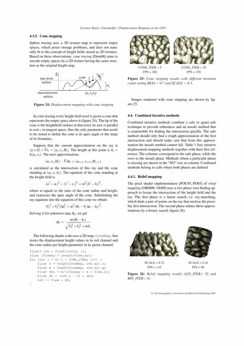
4.3.5. Cone stepping
Sphere tracing uses a 3D texture map to represent emptyspaces, which poses storage problems, and does not natu-rally fit to the concept of height fields stored as 2D textures.Based on these observations, cone tracing [Dum06] aims toencode empty spaces by a 2D texture having the same struc-ture as the original height map.
N
macrostructure surface
123
max levelsurface
(u ,v ,h )i ii
Hi
cone
Figure 24: Displacement mapping with cone stepping
In cone tracing every height field texel is given a cone thatrepresents the empty space above it (figure 24). The tip of thecone is the heightfield surface at that texel, its axis is parallelto axis z in tangent space, thus the only parameter that needsto be stored to define the cone is its apex angle or the slopeof its boundary.
Suppose that the current approximation on the ray is(u,v,0) +~Vti = (ui,vi,Hi). The height at this point is hi =h(ui,vi). The next approximation,
(ui,vi,Hi)−~V ∆ti = (ui+1,vi+1,Hi+1),
is calculated as the intersection of this ray and the conestanding at (ui,vi,hi). The equation of the cone standing atthe height field is
(u′−ui)2 +(v′− vi)
2 = m2(h′−hi)2,
where m equals to the ratio of the cone radius and height,and expresses the apex angle of the cone. Substituting theray equation into the equation of this cone we obtain
(V 2x +V 2
y )∆t2i = m2(Hi−Vz∆ti−hi)
2.
Solving it for unknown step ∆ti, we get
∆ti =m(Hi−hi)√
V 2x +V 2
y +mVz
The following shader code uses a 2D map, ConeMap, thatstores the displacement height values in its red channel andthe cone radius per height parameter in its green channel:
float3 uvh = float3(uvin, 1);float lViewxy = length(View.xy);for (int i = 0; i < CONE_ITER; i++) {
float h = tex2D(ConeMap, uvh.xy).r;float m = tex2D(ConeMap, uvh.xy).g;float dts = m/(lViewxy + m * View.z);float dt = (uvh.z - h) * dts;uvh -= View * dt;
}
CONE_ITER = 5 CONE_ITER = 30FPS = 380 FPS = 150
Figure 25: Cone stepping results with different iterationcount setting BIAS = 0.7 and SCALE = 0.3.
Images rendered with cone stepping are shown by fig-ure 25.
4.4. Combined iterative methods
Combined iterative methods combine a safe or quasi-safetechnique to provide robustness and an unsafe method thatis responsible for finding the intersection quickly. The safemethod should only find a rough approximation of the firstintersection and should make sure that from this approxi-mation the unsafe method cannot fail. Table 1 lists iterativedisplacement mapping methods together with their first ref-erence. The columns correspond to the safe phase, while therows to the unsafe phase. Methods where a particular phaseis missing are shown in the “NO” row or column. Combinedmethods belong to cells where both phases are defined.
4.4.1. Relief mapping
The pixel shader implementation [POC05, PO05] of reliefmapping [OBM00, Oli00] uses a two phase root-finding ap-proach to locate the intersection of the height field and theray. The first phase is a linear search, i.e. ray-marching,which finds a pair of points on the ray that enclose the possi-bly first intersection. The second phase refines these approx-imations by a binary search (figure 26).
SCALE = 0.32 SCALE = 0.16FPS = 110 FPS = 80
Figure 26: Relief mapping results (LIN_ITER= 32 andBIN_ITER= 4)
c© The Eurographics Association and Blackwell Publishing 2008.
Szirmay-Kalos, Umenhoffer / Displacement Mapping on the GPU
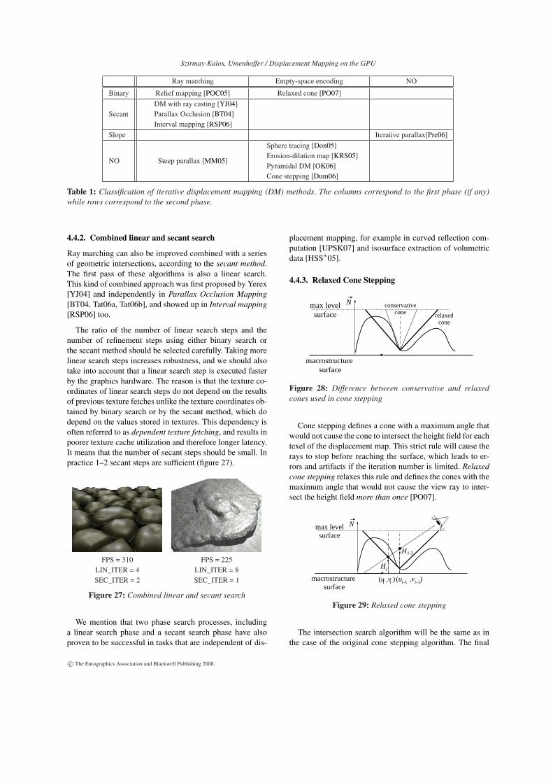
Ray marching Empty-space encoding NO
Binary Relief mapping [POC05] Relaxed cone [PO07]
SecantDM with ray casting [YJ04]Parallax Occlusion [BT04]Interval mapping [RSP06]
Slope Iterative parallax[Pre06]
NO Steep parallax [MM05]
Sphere tracing [Don05]Erosion-dilation map [KRS05]Pyramidal DM [OK06]Cone stepping [Dum06]
Table 1: Classification of iterative displacement mapping (DM) methods. The columns correspond to the first phase (if any)while rows correspond to the second phase.
4.4.2. Combined linear and secant search
Ray marching can also be improved combined with a seriesof geometric intersections, according to the secant method.The first pass of these algorithms is also a linear search.This kind of combined approach was first proposed by Yerex[YJ04] and independently in Parallax Occlusion Mapping[BT04, Tat06a, Tat06b], and showed up in Interval mapping[RSP06] too.
The ratio of the number of linear search steps and thenumber of refinement steps using either binary search orthe secant method should be selected carefully. Taking morelinear search steps increases robustness, and we should alsotake into account that a linear search step is executed fasterby the graphics hardware. The reason is that the texture co-ordinates of linear search steps do not depend on the resultsof previous texture fetches unlike the texture coordinates ob-tained by binary search or by the secant method, which dodepend on the values stored in textures. This dependency isoften referred to as dependent texture fetching, and results inpoorer texture cache utilization and therefore longer latency.It means that the number of secant steps should be small. Inpractice 1–2 secant steps are sufficient (figure 27).
FPS = 310 FPS = 225LIN_ITER = 4 LIN_ITER = 8SEC_ITER = 2 SEC_ITER = 1
Figure 27: Combined linear and secant search
We mention that two phase search processes, includinga linear search phase and a secant search phase have alsoproven to be successful in tasks that are independent of dis-
placement mapping, for example in curved reflection com-putation [UPSK07] and isosurface extraction of volumetricdata [HSS∗05].
4.4.3. Relaxed Cone Stepping
N
macrostructure surface
relaxedcone
max levelsurface
conservativecone
Figure 28: Difference between conservative and relaxedcones used in cone stepping
Cone stepping defines a cone with a maximum angle thatwould not cause the cone to intersect the height field for eachtexel of the displacement map. This strict rule will cause therays to stop before reaching the surface, which leads to er-rors and artifacts if the iteration number is limited. Relaxedcone stepping relaxes this rule and defines the cones with themaximum angle that would not cause the view ray to inter-sect the height field more than once [PO07].
N
macrostructure surface
max levelsurface
H i-1
(u ,v )(u ,v ) i-1i i i-1
Hi
Figure 29: Relaxed cone stepping
The intersection search algorithm will be the same as inthe case of the original cone stepping algorithm. The final
c© The Eurographics Association and Blackwell Publishing 2008.
Szirmay-Kalos, Umenhoffer / Displacement Mapping on the GPU
two search results will give an undershooting and an over-shooting points. From these points binary [PO07] or secantsearch can be started to find the exact solution.
5. Silhouette processing
So far we have discussed algorithms that compute the tex-ture coordinates of the visible point assuming a planarmacrostructure surface. For triangle meshes, the underly-ing macrostructure geometry might change and the modifiedtexture coordinates get outside of the texture footprint of thepolygon, thus the texture coordinate modification computedwith the planar assumption may become invalid. Anotherproblem is that the mesostructure surface may get projectedto more pixels than the macrostructure surface, but the frag-ment shader is invoked only if the macrostructure trianglepasses the backface culling, its processed point is projectedonto this pixel and passes the early z-test. Thus it can happenthat a height map point is ignored because its correspondingpoint of the macrostructure geometry is not processed by thefragment shader. These issues are particularly important attriangle edges between a front facing and a back facing poly-gons, which are responsible for the silhouettes of the detailedobject.
To cope with this problem, a simple silhouette processingapproach would discard the fragment if the modified tex-ture coordinate gets outside of texture space of the renderedpolygon. While this is easy to test for rectangles, the checkbecomes more complicated for triangles, and is not robustfor meshes that are tessellations of curved surfaces.
For meshes, instead of assuming a planar surface, i.e. alinear approximation, the local curvature information shouldalso be considered, and at least a quadratic approximationshould be used to describe the surface farther from the pro-cessed point. On the other hand, to activate the fragmentshader even for those pixels where the mesostructure sur-face is visible but the macrostructure surface is not, themacrostructure surface should be “thickened” to include alsothe volume of the height field above it. Of course, the thick-ened macrostructure surface must also be simple, otherwisethe advantages of displacement mapping get lost. Such ap-proaches are discussed in this section.
5.1. Silhouette processing for curved surfaces
In order to get better silhouettes, we have to locally deformthe height field according to the curvature of the smooth ge-ometry [OP05]. The mesostructure geometry~r(u,v) is usu-ally approximated locally by a quadrics [SYL02] in tangentspace (compare this second order approximation to the firstorder approximation of equation 3):
~r(u,v)≈~q(u,v) =~r(u0,v0)+ [u−u0,v− v0] ·
∂~r∂u
∂~r∂v
+
12· [u−u0,v− v0] ·
∂2~r∂u2
∂2~r∂u∂v
∂2~r∂u∂v
∂2~r∂v2
·
[u−u0v− v0
].
where all partial derivatives are evaluated at (u0,v0). If(u0,v0) corresponds to a vertex of the tessellated mesh, then
~r(u0,v0) = ~p(u0,v0),∂~r∂u
= ~T ,∂~r∂v
= ~B.
Matrix
H =
∂2~r∂u2
∂2~r∂u∂v
∂2~r∂u∂v
∂2~r∂v2
is a Hessian matrix. The eigenvalues of this matrix corre-spond to the principal curvatures and the eigenvectors to theprincipal curvature directions.
The second order approximation is the sum of the lin-ear form represented by the macrostructure mesh and aquadratic form
~q(u,v)≈ ~p(u,v)+12· [u−u0,v− v0] ·H · [u−u0,v− v0]
T .
Let us transform this quadratic surface to tangent space,and consider only the third coordinate hq representing theheight function of the quadratic surface:
hq(u,v) = (~q(u,v)−~p(u,v)) ·~N0 =
a(u−u0)2 +b(u−u0)(v− v0)+ c(v− v0)
2. (13)
The elements of the Hessian matrix and parameters a,b,ccan be computed analytically if the parametric equation ofthat surface which has been tessellated is known (this is thecase if we tessellate a sphere, a cylinder, etc.). If only the tes-sellated surface is available, then the derivatives should bedetermined directly from the mesh around vertex ~p0. Let ussuppose that the vertices of the triangles incident to ~p0 are(u0,v0,h0),(u1,v1,h1), . . . ,(un,vn,hn) in the tangent spaceattached to ~p0. Substituting these points to the quadratic ap-proximation we obtain for i = 1, . . . ,n
hi ≈ a(ui−u0)2 +b(ui−u0)(vi− v0)+ c(vi− v0)
2.
since h0 = 0 in the tangent space of ~p0. This is a linear sys-tem
e = A ·x,
where e = [h1, . . . ,hn]T is an n-element vector,
A =
(u1−u0)2, (u1−u0)(v1− v0), (v1− v0)2
......
...(un−u0)2, (un−u0)(vn− v0), (vn− v0)2
c© The Eurographics Association and Blackwell Publishing 2008.
Szirmay-Kalos, Umenhoffer / Displacement Mapping on the GPU
is an n-row, 3-column matrix, and
x =
abc
.
is a three-element vector. Note that the number of equationsis n > 3 and just three unknowns exist, thus the equationis overdetermined. An approximate solution with minimalleast-squares error can be obtained with the pseudo inversemethod:
x = (AT ·A)−1 ·AT · e.
Note that just a 3×3 matrix needs to be inverted.
Having determined parameters a,b,c the height of thequadratic approximation of the smooth surface is obtainedusing equation 13.
(u,v)
N
h
Original tangent space
(u,v)
N
T, B
Warped tangent space
ray
ray
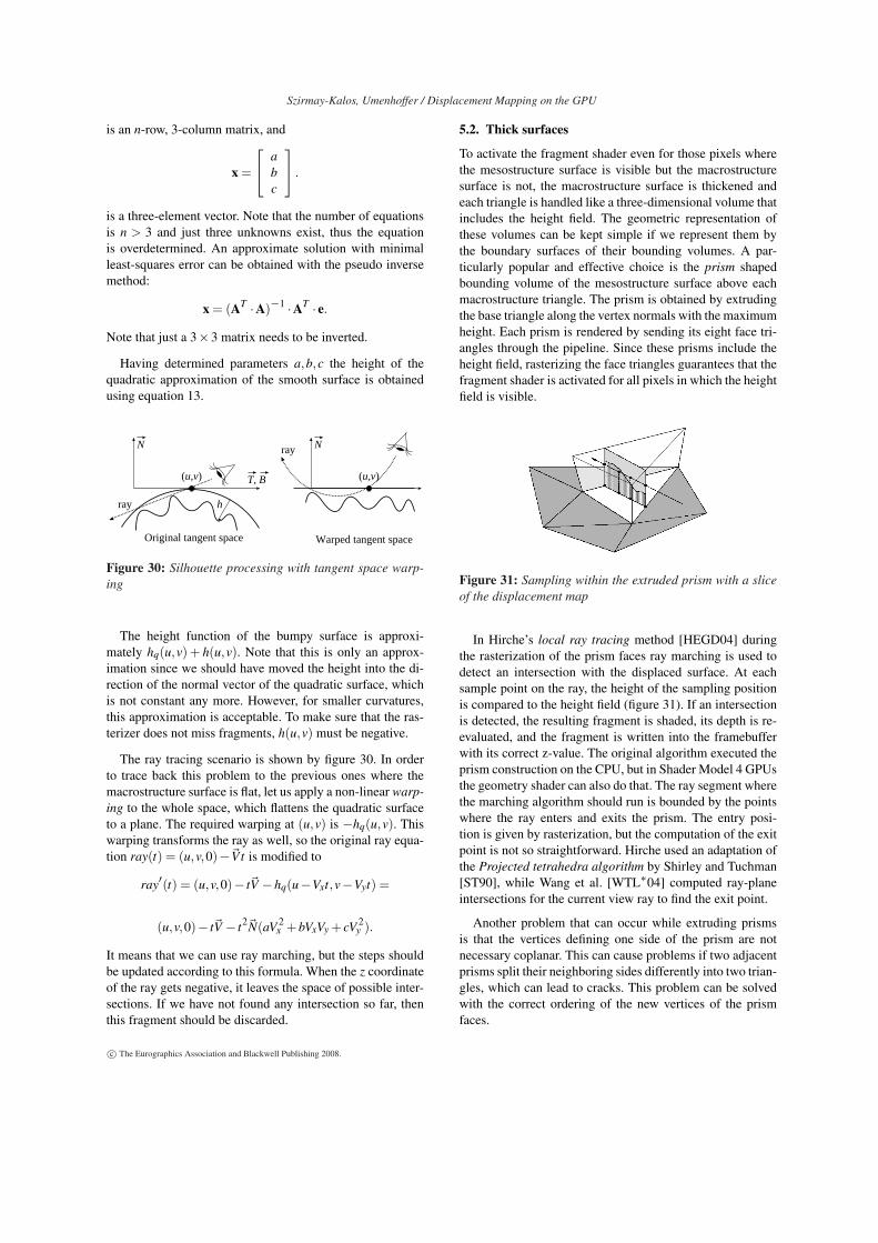
Figure 30: Silhouette processing with tangent space warp-ing
The height function of the bumpy surface is approxi-mately hq(u,v) + h(u,v). Note that this is only an approx-imation since we should have moved the height into the di-rection of the normal vector of the quadratic surface, whichis not constant any more. However, for smaller curvatures,this approximation is acceptable. To make sure that the ras-terizer does not miss fragments, h(u,v) must be negative.
The ray tracing scenario is shown by figure 30. In orderto trace back this problem to the previous ones where themacrostructure surface is flat, let us apply a non-linear warp-ing to the whole space, which flattens the quadratic surfaceto a plane. The required warping at (u,v) is −hq(u,v). Thiswarping transforms the ray as well, so the original ray equa-tion ray(t) = (u,v,0)−~Vt is modified to
ray′(t) = (u,v,0)− t~V −hq(u−Vxt,v−Vyt) =
(u,v,0)− t~V − t2~N(aV 2x +bVxVy + cV 2
y ).
It means that we can use ray marching, but the steps shouldbe updated according to this formula. When the z coordinateof the ray gets negative, it leaves the space of possible inter-sections. If we have not found any intersection so far, thenthis fragment should be discarded.
5.2. Thick surfaces
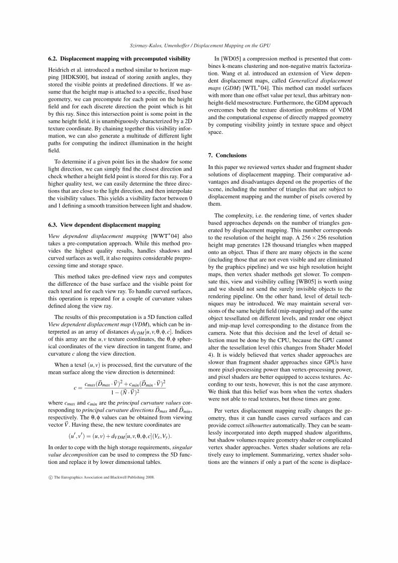
To activate the fragment shader even for those pixels wherethe mesostructure surface is visible but the macrostructuresurface is not, the macrostructure surface is thickened andeach triangle is handled like a three-dimensional volume thatincludes the height field. The geometric representation ofthese volumes can be kept simple if we represent them bythe boundary surfaces of their bounding volumes. A par-ticularly popular and effective choice is the prism shapedbounding volume of the mesostructure surface above eachmacrostructure triangle. The prism is obtained by extrudingthe base triangle along the vertex normals with the maximumheight. Each prism is rendered by sending its eight face tri-angles through the pipeline. Since these prisms include theheight field, rasterizing the face triangles guarantees that thefragment shader is activated for all pixels in which the heightfield is visible.
Figure 31: Sampling within the extruded prism with a sliceof the displacement map
In Hirche’s local ray tracing method [HEGD04] duringthe rasterization of the prism faces ray marching is used todetect an intersection with the displaced surface. At eachsample point on the ray, the height of the sampling positionis compared to the height field (figure 31). If an intersectionis detected, the resulting fragment is shaded, its depth is re-evaluated, and the fragment is written into the framebufferwith its correct z-value. The original algorithm executed theprism construction on the CPU, but in Shader Model 4 GPUsthe geometry shader can also do that. The ray segment wherethe marching algorithm should run is bounded by the pointswhere the ray enters and exits the prism. The entry posi-tion is given by rasterization, but the computation of the exitpoint is not so straightforward. Hirche used an adaptation ofthe Projected tetrahedra algorithm by Shirley and Tuchman[ST90], while Wang et al. [WTL∗04] computed ray-planeintersections for the current view ray to find the exit point.
Another problem that can occur while extruding prismsis that the vertices defining one side of the prism are notnecessary coplanar. This can cause problems if two adjacentprisms split their neighboring sides differently into two trian-gles, which can lead to cracks. This problem can be solvedwith the correct ordering of the new vertices of the prismfaces.
c© The Eurographics Association and Blackwell Publishing 2008.

Szirmay-Kalos, Umenhoffer / Displacement Mapping on the GPU
Dufort et al. used a voxel traversal algorithm inside thebounding prism [DLP05]. This method can simulate dis-placement maps as well as semitransparent surface details,including several surface shading effects (visual masking,self-shadowing, absorption of light) at interactive rates.
The idea of mapping a three-dimensional volume onto asurface with prisms also showed up in shell maps [PBFJ05].
5.2.1. Shader Model 4 adaptation of the local raytracing method
The displacement techniques using bounding prisms can beimplemented purely in hardware with the geometry shaderannounced in Shader Model 4. One possible Diret3D 10 im-plementation can be found in the DirectX SDK 2006 August.
The prism extrusion and the ray exit point calculation aredone in the geometry shader. The geometry shader reads thetriangle data (three vertices) and creates additional trianglesforming a prism with edge extrusion. It splits the prism intothree tetrahedra just like in [HEGD04]. For each vertex of atetrahedron, the distance from the “rear” of the tetrahedron iscomputed. Then the triangles with these additional data arepassed to the clipping and rasterizer units. From the raster-izer the fragment shader gets the entry point and its texturecoordinate, as well as the exit point and its texture coordi-nates, which are interpolated by the rasterizer from the dis-tance values computed by the geometry shader.
Figure 32: Displacement mapping with local ray tracing im-plemented on the geometry shader of a NVidia 8800 GPUand rendered at 200 FPS
Figure 32 has been rendered with this algorithm on aShader Model 4 compatible GPU.
6. Self-shadowing computation
Self-shadowing can be easily added to iterative fragmentshader methods. By calling it with the Light vector (point-ing from the shaded point to the light source) instead of theView vector, it is possible to decide whether the shaded point
is in shadow or not (figure 33). Using more than one lightvector per light source, even soft shadows can be generated[Tat06a, Tat06b].
FPS = 100 FPS = 50
FPS = 60 FPS = 30
FPS = 85 FPS = 42
Figure 33: The secant method without (left) and with self-shadowing (right) setting LIN_ITER = 32, SEC_ITER = 4
We note that shadows can also be burnt into the in-formation associated with the texels, as happens in thecase of bi-directional texture functions. Bi-directional tex-ture functions have been introduced by Dana et al.[DGNK97, SBLD03, MGW01, HDKS00]. An excellent re-view of the acquisition, synthesis, and rendering of bi-directional texture functions can be found in [MMS∗04].
6.1. Horizon mapping
Another fast method for self-shadowing computation is hori-zon mapping [Max88]. The idea behind horizon mapping isto precompute the angle to the horizon in a discrete numberof directions. Horizon angles represent at what height thesky becomes visible at the given direction (i.e. passes overthe horizon). This parametrization can be used to producethe self-shadowing of geometry. An extension of this algo-rithm also considered the local geometry [SC00].
c© The Eurographics Association and Blackwell Publishing 2008.
Szirmay-Kalos, Umenhoffer / Displacement Mapping on the GPU
6.2. Displacement mapping with precomputed visibility
Heidrich et al. introduced a method similar to horizon map-ping [HDKS00], but instead of storing zenith angles, theystored the visible points at predefined directions. If we as-sume that the height map is attached to a specific, fixed basegeometry, we can precompute for each point on the heightfield and for each discrete direction the point which is hitby this ray. Since this intersection point is some point in thesame height field, it is unambiguously characterized by a 2Dtexture coordinate. By chaining together this visibility infor-mation, we can also generate a multitude of different lightpaths for computing the indirect illumination in the heightfield.
To determine if a given point lies in the shadow for somelight direction, we can simply find the closest direction andcheck whether a height field point is stored for this ray. For ahigher quality test, we can easily determine the three direc-tions that are close to the light direction, and then interpolatethe visibility values. This yields a visibility factor between 0and 1 defining a smooth transition between light and shadow.
6.3. View dependent displacement mapping
View dependent displacement mapping [WWT∗04] alsotakes a pre-computation approach. While this method pro-vides the highest quality results, handles shadows andcurved surfaces as well, it also requires considerable prepro-cessing time and storage space.
This method takes pre-defined view rays and computesthe difference of the base surface and the visible point foreach texel and for each view ray. To handle curved surfaces,this operation is repeated for a couple of curvature valuesdefined along the view ray.
The results of this precomputation is a 5D function calledView dependent displacement map (VDM), which can be in-terpreted as an array of distances dV DM [u,v,θ,φ,c]. Indicesof this array are the u,v texture coordinates, the θ,φ spher-ical coordinates of the view direction in tangent frame, andcurvature c along the view direction.
When a texel (u,v) is processed, first the curvature of themean surface along the view direction is determined:
c =cmax(~Dmax ·~V )2 + cmin(~Dmin ·~V )2
1− (~N ·~V )2
where cmax and cmin are the principal curvature values cor-responding to principal curvature directions ~Dmax and ~Dmin,respectively. The θ,φ values can be obtained from viewingvector ~V . Having these, the new texture coordinates are
(u′,v′) = (u,v)+dV DM [u,v,θ,φ,c](Vx,Vy).
In order to cope with the high storage requirements, singularvalue decomposition can be used to compress the 5D func-tion and replace it by lower dimensional tables.
In [WD05] a compression method is presented that com-bines k-means clustering and non-negative matrix factoriza-tion. Wang et al. introduced an extension of View depen-dent displacement maps, called Generalized displacementmaps (GDM) [WTL∗04]. This method can model surfaceswith more than one offset value per texel, thus arbitrary non-height-field mesostructure. Furthermore, the GDM approachovercomes both the texture distortion problems of VDMand the computational expense of directly mapped geometryby computing visibility jointly in texture space and objectspace.
7. Conclusions
In this paper we reviewed vertex shader and fragment shadersolutions of displacement mapping. Their comparative ad-vantages and disadvantages depend on the properties of thescene, including the number of triangles that are subject todisplacement mapping and the number of pixels covered bythem.
The complexity, i.e. the rendering time, of vertex shaderbased approaches depends on the number of triangles gen-erated by displacement mapping. This number correspondsto the resolution of the height map. A 256× 256 resolutionheight map generates 128 thousand triangles when mappedonto an object. Thus if there are many objects in the scene(including those that are not even visible and are eliminatedby the graphics pipeline) and we use high resolution heightmaps, then vertex shader methods get slower. To compen-sate this, view and visibility culling [WB05] is worth usingand we should not send the surely invisible objects to therendering pipeline. On the other hand, level of detail tech-niques may be introduced. We may maintain several ver-sions of the same height field (mip-mapping) and of the sameobject tessellated on different levels, and render one objectand mip-map level corresponding to the distance from thecamera. Note that this decision and the level of detail se-lection must be done by the CPU, because the GPU cannotalter the tessellation level (this changes from Shader Model4). It is widely believed that vertex shader approaches areslower than fragment shader approaches since GPUs havemore pixel-processing power than vertex-processing power,and pixel shaders are better equipped to access textures. Ac-cording to our tests, however, this is not the case anymore.We think that this belief was born when the vertex shaderswere not able to read textures, but those times are gone.
Per vertex displacement mapping really changes the ge-ometry, thus it can handle cases curved surfaces and canprovide correct silhouettes automatically. They can be seam-lessly incorporated into depth mapped shadow algorithms,but shadow volumes require geometry shader or complicatedvertex shader approaches. Vertex shader solutions are rela-tively easy to implement. Summarizing, vertex shader solu-tions are the winners if only a part of the scene is displace-
c© The Eurographics Association and Blackwell Publishing 2008.

Szirmay-Kalos, Umenhoffer / Displacement Mapping on the GPU
texture mapping bump mapping parallax mapping
parallax mapping with offset limiting parallax mapping with slope iterative parallax mapping
ray marching binary search sphere tracing
relief mapping cone stepping per-vertex displacement mapping
Figure 34: Comparison of mapping techniques assuming normal displacement sizes
ment mapped, or we apply view culling or level of detailtechniques, or if the displacements are really large.
The rendering time of fragment shader approaches de-pends on the number of pixels covering the displacementmapped objects. Thus if we usually get far from these objectsor the objects are not visible, then fragment shader methodsare faster than vertex shader techniques.
Fragment shader methods are approximate by nature, al-though different algorithms take different compromises be-tween accuracy and speed. An accurate solution that handlessilhouettes as well is quite difficult to implement, and the im-plementation is rather slow. Thus fragment shader solutionsare viable if the height map has high frequency characteris-
tics, and thus has high resolution, and the objects are small(i.e. usually cover just a smaller part of the screen), and thedisplacements are also small, so approximation errors are notso visible.
Displacement mapping also has limitations. For example,it is constrained to a one-valued height field so holes can-not be added. This restriction is addressed by Deformationdisplacement mapping [Elb02, SKE05] and Generalized dis-placement mapping [WTL∗04]. However, despite to its limi-tations, it has become a popular technique and we can expectits increasing role in games and real-time systems.
c© The Eurographics Association and Blackwell Publishing 2008.

Szirmay-Kalos, Umenhoffer / Displacement Mapping on the GPU
ray marching binary search sphere tracing
relief mapping cone stepping per-vertex displacement mapping
Figure 35: Comparison of high quality mapping techniques assuming extreme displacement sizes
8. Acknowledgement
This work has been supported by the GameTools FP6 (IST-2-004363) project, Hewlett-Packard, and the National Officefor Research and Technology (Hungary).
References
[APS00] ASHIKHMIN M., PREMOZE S., SHIRLEY P.: Amicrofacet-based BRDF generator. In SIGGRAPH 2000Proceedings (2000), Akeley K., (Ed.), pp. 65–74.
[ATI03] ATI: Normalmapper tool, 2003. Avail-able: http://www2.ati.com/developer/NormalMapper-3_2_2.zip.
[BERW97] BENNEBROEK K., ERNST I., RÜSSELER H.,WITTING O.: Design principles of hardware-based Phongshading and bump-mapping. Computers and Graphics 21,2 (1997), 143–149.
[Bla92] BLASCO O.: Curvature simulation using normalmaps. In Game Programming Gems III, Treglia D., (Ed.).Charles River Media, Boston, 1992, pp. 433–443.
[Bli77] BLINN J. F.: Models of light reflection for com-puter synthesized pictures. In Computer Graphics (SIG-GRAPH ’77 Proceedings) (1977), pp. 192–198.
[Bli78] BLINN J. F.: Simulation of wrinkled surfaces.In Computer Graphics (SIGGRAPH ’78 Proceedings)(1978), pp. 286–292.
[Bly06] BLYTHE D.: The Direct3D 10 system. In SIG-GRAPH 2006 Proceedings (2006), pp. 724–734.
[BM93] BECKER B. G., MAX N. L.: Smooth transitionsbetween bump rendering algorithms. In SIGGRAPH ’93Proceedings (1993), ACM Press, pp. 183–190.
[BN76] BLINN J. F., NEWELL M. E.: Texture and reflec-tion in computer generated images. Communications ofthe ACM 19, 10 (1976), 542–547.
[BS05] BOUBEKEUR T., SCHLICK C.: Generic mesh re-finement on GPU. In HWWS ’05: Proceedings of the ACMSIGGRAPH/EUROGRAPHICS conference on Graphicshardware (2005), ACM Press, pp. 99–104.
[BT04] BRAWLEY Z., TATARCHUK N.: Parallax occlu-sion mapping: Self-shadowing, perspective-correct bumpmapping using reverse height map tracing. In ShaderX3:Advanced Rendering Techniques in DirectX and OpenGL,Engel W., (Ed.). Charles River Media, Cambridge, MA,2004.
[Cat74] CATMULL E.: A Subdivision Algorithm for Com-puter Display and Curved Surfaces. PhD thesis, Univer-sity of Utah, Salt Lake City, Utah, 1974. Ph.D. Disserta-tion.
[CCC87] COOK R. L., CARPENTER L., CATMULL E.:The reyes image rendering architecture. In ComputerGraphics (SIGGRAPH ’87 Proceedings) (1987), pp. 95–102.
[CG85] CAREY R. J., GREENBERG D. P.: Textures forrealistic image synthesis. Computers and Graphics 9, 2(1985), 125–138.
[CMSR98] CIGNONI P., MONTANI C., SCOPIGNO R.,ROCCHINI C.: A general method for preserving at-tribute values on simplified meshes. In IEEE Visualization(1998), pp. 59–66.
[Coo84] COOK R. L.: Shade trees. In SIGGRAPH ’84Proceedings (1984), ACM Press, pp. 223–231.
[CORLS96] COHEN-OR D., RICH E., LERNER U.,
c© The Eurographics Association and Blackwell Publishing 2008.
Szirmay-Kalos, Umenhoffer / Displacement Mapping on the GPU
SHENKAR V.: A Real-Time Photo-Realistic Visual Fly-through. IEEE Transactions on Visualization and Com-puter Graphics 2, 3 (1996), 255–264.
[Cro77] CROW F. C.: Shadow algorithm for computergraphics. In Computer Graphics (SIGGRAPH ’77 Pro-ceedings) (1977), pp. 242–248.
[CT81] COOK R., TORRANCE K.: A reflectance modelfor computer graphics. Computer Graphics 15, 3 (1981),7–24.
[Dan80] DANIELSSON P.: Euclidean distance mapping.Computer Graphics and Image Processing 14 (1980),227–248.
[DGNK97] DANA K., GINNEKEN B., NAYAR S., KOEN-DERINK J.: Reflectance and texture of real-world sur-faces. ACM Transactions on Graphics 18, 1 (1997), 1–34.
[DH00] DOGGETT M., HIRCHE J.: Adaptive view depen-dent tessellation of displacement maps. In HWWS ’00:Proceedings of the ACM SIGGRAPH/EUROGRAPHICSworkshop on Graphics hardware (2000), ACM Press,pp. 59–66.
[Die00] DIETRICH S.: Elevation Maps. NVIDIA Corpo-ration, 2000.
[DKS01] DOGGETT M. C., KUGLER A., STRASSER W.:Displacement mapping using scan conversion hardwarearchitectures. Computer Graphics Forum 20, 1 (2001),13–26.
[DLP05] DUFORT J.-F., LEBLANC L., POULIN P.: Inter-active rendering of meso-structure surface details usingsemi-transparent 3d textures. In Proc. Vision, Modeling,and Visualization 2005 (2005), pp. 399–406.
[Don05] DONELLY W.: Per-pixel displacement mappingwith distance functions. In GPU Gems 2, Parr M., (Ed.).Addison-Wesley, 2005, pp. 123–136.
[Dum06] DUMMER J.: Cone Step Mapping: An IterativeRay-Heightfield Intersection Algorithm. Tech. rep., 2006.http://www.lonesock.net/files/ConeStepMapping.pdf.
[EBAB05] ESPINO F. J., BÓO M., AMOR M.,BRUGUERA J. D.: Adaptive tessellation of béziersurfaces based on displacement maps. In The 13-thInternational Conference in Central Europe on ComputerGraphics, Visualization and Computer Vision (2005),pp. 29–32.
[Elb02] ELBER G.: Geometric deformation-displacementmaps. In PG ’02: Proceedings of the 10th Pacific Confer-ence on Computer Graphics and Applications (Washing-ton, DC, USA, 2002), IEEE Computer Society, p. 156.
[EY03] ELHELW M. A., YANG G.-Z.: Cylindrical relieftexture mapping. Journal of WSCG 11 (2003), 125–132.
[Fou92] FOURNIER A.: Filtering Normal Maps and Cre-ating Multiple Surfaces. Tech. rep., Vancouver, BC,Canada, 1992.
[Gat03] GATH J.: Derivation of the tangent spacematrix, 2003. http://www.blacksmith-studios.dk/projects/downloads/tangent_matrix_derivation.php.
[GH99] GUMHOLD S., HÜTTNER T.: Multiresolutionrendering with displacement mapping. In HWWS ’99:Proceedings of the ACM SIGGRAPH/EUROGRAPHICSworkshop on Graphics hardware (1999), ACM Press,pp. 55–66.
[Har93] HART J. C.: Sphere tracing: Simple robust an-tialiased rendering of distance-based implicit surfaces. InSIGGRAPH 93 Course Notes: Modeling, Visualizing, andAnimating Implicit Surfaces. 1993, pp. 14–1 to 14–11.
[HDKS00] HEIDRICH W., DAUBERT K., KAUTZ J., SEI-DEL H.-P.: Illuminating micro geometry based on pre-computed visibility. In SIGGRAPH 2000 Proceedings(2000), pp. 455–464.
[Hec86] HECKBERT P. S.: Survey of texture mapping.IEEE Computer Graphics and Applications 6, 11 (1986),56–67.
[HEGD04] HIRCHE J., EHLERT A., GUTHE S.,DOGGETT M.: Hardware accelerated per-pixel displace-ment mapping. In Proceedings of Graphics Interface(2004), pp. 153–158.
[HLHS03] HASENFRATZ J.-M., LAPIERRE M.,HOLZSCHUCH N., SILLION F. X.: A survey ofrealtime soft shadow algorithms. In EurographicsConference. State of the Art Reports (2003).
[HS98] HEIDRICH W., SEIDEL H.-P.: Ray-tracing proce-dural displacement shaders. In Proceedings of GraphicsInterface (1998), pp. 8–16.
[HS04] HENNING C., STEPHENSON P.: Accelerating theray tracing of height fields. In GRAPHITE ’04: Pro-ceedings of the 2nd international conference on Com-puter graphics and interactive techniques in Australia andSouth East Asia (2004), ACM Press, pp. 254–258.
[HSS∗05] HADWIGER M., SIGG C., SCHARSACH H.,BÜHLER K., GROSS M.: Real-time ray-casting and ad-vanced shading of discrete isosurfaces. In EurographicsConference (2005), pp. 303–312.
[HTSG91] HE X., TORRANCE K., SILLION F., GREEN-BERG D.: A comprehensive physical model for light re-flection. Computer Graphics 25, 4 (1991), 175–186.
[JWP05] JESCHKE S., WIMMER M., PURGATHOFER W.:Image-based representations for accelerated rendering ofcomplex scenes. In Eurographics, 2005. State of the ArtReports (2005), p. 61.
[Kil00] KILGARD M.: A practical and robustbump-mapping technique for today’s GPU’s, 2000.http://www.nvidia.com/.
[KKI∗01] KANEKO T., KAKAHEI T., INAMI M.,KAWAKAMI N., YANAGIDA Y., MAEDA T., TACHI S.:
c© The Eurographics Association and Blackwell Publishing 2008.
Szirmay-Kalos, Umenhoffer / Displacement Mapping on the GPU
Detailed shape representation with parallax mapping. InProceedings of ICAT 2001 (2001), pp. 205–208.
[KRS05] KOLB A., REZK-SALAMA C.: Efficient emptyspace skipping for per-pixel displacement mapping. InVision, Modeling and Visualization (2005).
[KS01] KAUTZ J., SEIDEL H.-P.: Hardware accelerateddisplacement mapping for image based rendering. In Pro-ceedings of Graphics Interface (2001), pp. 61–70.
[KSK01] KELEMEN C., SZIRMAY-KALOS L.: A micro-facet based coupled specular-matte BRDF model with im-portance sampling. In Eurographics 2001, Short papers,Manchester (2001), pp. 25–34.
[Lev90] LEVOY M.: Efficient ray tracing of volume data.ACM Transactions on Graphics 9, 3 (1990), 245–261.
[LKG∗03] LENSCH H. P. A., KAUTZ J., GOESELE M.,HEIDRICH W., SEIDEL H.-P.: Image-based reconstruc-tion of spatial appearance and geometric detail. ACMTransactions on Graphics 22, 2 (2003), 234–257.
[LP95] LOGIE J. R., PATTERSON J. W.: Inverse displace-ment mapping in the general case. Computer GraphicsForum 14, 5 (December 1995), 261–273.
[LPFH01] LENGYEL J., PRAUN E., FINKELSTEIN A.,HOPPE H.: Real-time fur over arbitrary surfaces. InProceedings of the 2001 Symposium on Interactive 3DGraphics (2001), ACM Press, pp. 227–232.
[LS95] LEE C.-H., SHIN Y. G.: An efficient ray trac-ing method for terrain rendering. In Pacific Graphics ’95(1995), pp. 183–193.
[Max88] MAX N.: Horizon mapping: Shadows for bump-mapped surfaces. The Visual Computer 4, 2 (1988), 109–117.
[MGW01] MALZBENDER T., GELB D., WOLTERS H.:Polynomial texture maps. In SIGGRAPH 2001 Proceed-ings (2001), pp. 519–528.
[MJW07] MANTLER S., JESCHKE S., WIMMER M.: Dis-placement Mapped Billboard Clouds. Tech. Rep. TR-186-2-07-01, Jan. 2007.
[MM02] MOULE K., MCCOOL M.: Efficient boundedadaptive tessellation of displacement maps. In Proceed-ings of the Graphics Interface (2002), pp. 171–180.
[MM05] MCGUIRE M., MCGUIRE M.: Steepparallax mapping. In I3D 2005 Poster (2005).http://www.cs.brown.edu/research/graphics/games/SteepParallax/index.htm.
[MMS∗04] MUELLER G., MESETH J., SATTLER M.,SARLETTE R., KLEIN R.: Acquisition, synthesis and ren-dering of bidirectional texture functions. In Eurographics2004, State of the art reports (2004).
[Mus88] MUSGRAVE F. K.: Grid tracing: Fast ray tracingfor height fields. Research Report YALEU/DCS/RR-639(1988).
[OB99] OLIVEIRA M. M., BISHOP G.: Relief Textures.Tech. rep., Chapel Hill, NC, USA, 1999.
[OBM00] OLIVEIRA M. M., BISHOP G., MCALLISTER
D.: Relief texture mapping. In SIGGRAPH 2000 Pro-ceedings (2000), pp. 359–368.
[OK06] OH K., KI H., LEE C.-H.: Pyramidal displace-ment mapping: A GPU-based atrifacts-free ray tracingthrough an image pyramid. In ACM Symposium on Vir-tual Reality Software and Technology (VRST’06) (2006),pp. 75–82.
[Oli00] OLIVEIRA M. M.: Relief Texture Mapping. PhDthesis, University of North Carolina, 2000.
[OP05] OLIVEIRA M. M., POLICARPO F.: An EfficientRepresentation for Surface Details. Tech. rep., 2005.UFRGS Technical Report RP-351.
[PAC97] PEERCY M., AIREY J., CABRAL B.: Efficientbump mapping hardware. In SIGGRAPH 97 Proceedings(1997), pp. 303–306.
[PBFJ05] PORUMBESCU S. D., BUDGE B., FENG L.,JOY K. I.: Shell maps. In SIGGRAPH 2005 Proceed-ings (2005), pp. 626–633.
[PH96] PHARR M., HANRAHAN P.: Geometry cachingfor ray-tracing displacement maps. In EurographicsRendering Workshop 1996 Proceedings (1996), SpringerWien, pp. 31–40.
[PHL91] PATTERSON J. W., HOGGAR S. G., LOGIE
J. R.: Inverse displacement mapping. Computer GraphicsForum 10, 2 (1991), 129–139.
[PO05] POLICARPO F., OLIVEIRA M. M.: Renderingsurface details with relief mapping. In ShaderX4: Ad-vanced Rendering Techniques, Engel W., (Ed.). CharlesRiver Media, 2005.
[PO07] POLICARPO F., OLIVEIRA M. M.: Relaxed conestepping for relief mapping. In GPU Gems 3, Nguyen H.,(Ed.). Addison Wesley, 2007.
[POC05] POLICARPO F., OLIVEIRA M. M., COMBA J.:Real-time relief mapping on arbitrary polygonal surfaces.In ACM SIGGRAPH 2005 Symposium on Interactive 3DGraphics and Games (2005), pp. 155–162.
[Pre06] PREMECZ M.: Iterative parallax mapping withslope information. In Central European Seminar on Com-puter Graphics (2006). http://www.cescg.org/CESCG-2006/papers/TUBudapest-Premecz-Matyas.pdf.
[PRZ05] PARILOV E., ROSENBERG I., ZORIN D.: Real-time rendering of normal maps with discontinuities. Tech.rep., 2005. CIMS.
[PS02] PARILOV S., STÜRZLINGER W.: Layered relieftextures. In WSCG Proceedings (2002), pp. 357–364.
[QQZ∗03] QU H., QIU F., ZHANG N., KAUFMAN A.,WAN M.: Ray tracing height fields. In Computer Graph-ics International (2003), pp. 202–209.
c© The Eurographics Association and Blackwell Publishing 2008.
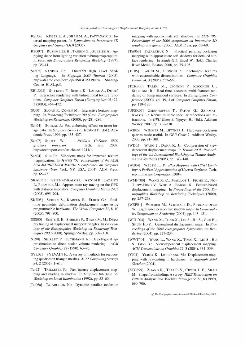
Szirmay-Kalos, Umenhoffer / Displacement Mapping on the GPU
[RSP06] RISSER E. A., SHAH M. A., PATTANAIK S.: In-terval mapping poster. In Symposium on Interactive 3DGraphics and Games (I3D) (2006).
[RTG97] RUSHMEIER H., TAUBIN G., GUEZIEZ A.: Ap-plying shape from lighting variation to bump map capture.In Proc. 8th Eurographics Rendering Workshop (1997),pp. 35–44.
[San05] SANDER P.: DirectX9 High Level Shad-ing Language. In Siggraph 2005 Tutorial (2005).http://ati.amd.com/developer/SIGGRAPH05/ Shading-Course_HLSL.pdf.
[SBLD03] SUYKENS F., BERGE K., LAGAE A., DUTRÉ
P.: Interactive rendering with bidirectional texture func-tions. Computer Graphics Forum (Eurographics 03) 22,3 (2003), 464–472.
[SC00] SLOAN P., COHEN M.: Interactive horizon map-ping. In Rendering Techniques ’00 (Proc. EurographicsWorkshop on Rendering) (2000), pp. 281–286.
[Sch94] SCHLAG J.: Fast embossing effects on raster im-age data. In Graphics Gems IV, Heckbert P., (Ed.). Aca-demic Press, 1994, pp. 433–437.
[Sco07] SCOTT W.: Nvidia’s GeForce 8800graphics processor. Tech. rep., 2007.http://techreport.com/articles.x/11211/1.
[Sen04] SEN P.: Silhouette maps for improved texturemagnification. In HWWS ’04: Proceedings of the ACMSIGGRAPH/EUROGRAPHICS conference on Graphicshardware (New York, NY, USA, 2004), ACM Press,pp. 65–73.
[SKALP05] SZIRMAY-KALOS L., ASZÓDI B., LAZÁNYI
I., PREMECZ M.: Approximate ray-tracing on the GPUwith distance impostors. Computer Graphics Forum 24, 3(2005), 695–704.
[SKE05] SCHEIN S., KARPEN E., ELBER G.: Real-time geometric deformation displacement maps usingprogrammable hardware. The Visual Computer 21, 8–10(2005), 791–800.
[SSS00] SMITS B. E., SHIRLEY P., STARK M. M.: Directray tracing of displacement mapped triangles. In Proceed-ings of the Eurographics Workshop on Rendering Tech-niques 2000 (2000), Springer-Verlag, pp. 307–318.
[ST90] SHIRLEY P., TUCHMANN A.: A polygonal ap-proximation to direct scalar volume rendering. ACMComputer Graphics 24 (1990), 63–70.
[SYL02] SYLVAIN P.: A survey of methods for recover-ing quadrics in triangle meshes. ACM Computing Surveys34, 2 (2002), 1–61.
[Tai92] TAILLEFER F.: Fast inverse displacement map-ping and shading in shadow. In Graphics Interface ’92Workshop on Local Illumination (1992), pp. 53–60.
[Tat06a] TATARCHUK N.: Dynamic parallax occlusion
mapping with approximate soft shadows. In SI3D ’06:Proceedings of the 2006 symposium on Interactive 3Dgraphics and games (2006), ACM Press, pp. 63–69.
[Tat06b] TATARCHUK N.: Practical parallax occlusionmapping with approximate soft shadows for detailed sur-face rendering. In ShaderX 5, Engel W., (Ed.). CharlesRiver Media, Boston, 2006, pp. 75–105.
[TC05] TARINI M., CIGNONI P.: Pinchmaps: Textureswith customizable discontinuities. Computer GraphicsForum 24, 3 (2005), 557–568.
[TCRS00] TARINI M., CIGNONI P., ROCCHINI C.,SCOPIGNO R.: Real time, accurate, multi-featured ren-dering of bump mapped surfaces. In Eurographics Con-ference (2000), vol. 19, 3 of Computer Graphics Forum,pp. 119–130.
[UPSK07] UMENHOFFER T., PATOW G., SZIRMAY-KALOS L.: Robust multiple specular reflections and re-fractions. In GPU Gems 3, Nguyen H., (Ed.). AddisonWesley, 2007, pp. 317–338.
[WB05] WIMMER M., BITTNER J.: Hardware occlusionqueries made useful. In GPU Gems 2. Addison-Wesley,2005, pp. 91–108.
[WD05] WANG J., DANA K. J.: Compression of viewdependent displacement maps. In Texture 2005: Proceed-ings of the 4th International Workshop on Texture Analy-sis and Synthesis (2005), pp. 143–148.
[Wel04] WELSH T.: Parallax Mapping with Offset Limit-ing: A PerPixel Approximation of Uneven Surfaces. Tech.rep., Infiscape Corporation, 2004.
[WMF∗00] WANG X. C., MAILLOT J., FIUME E., NG-THOW-HING V., WOO A., BAKSHI S.: Feature-baseddisplacement mapping. In Proceedings of the 2000 Eu-rographics Workshop on Rendering Techniques (2000),pp. 257–268.
[WSP04] WIMMER M., SCHERZER D., PURGATHOFER
W.: Light space perspective shadow maps. In Eurograph-ics Symposium on Rendering (2004), pp. 143–151.
[WTL∗04] WANG X., TONG X., LIN S., HU S., GUO B.,SHUM H.-Y.: Generalized displacement maps. In Pro-ceedings of the 2004 Eurographics Symposium on Ren-dering (2004), pp. 227–234.
[WWT∗04] WANG L., WANG X., TONG X., LIN S., HU
S., GUO B.: View-dependent displacement mapping.ACM Transactions on Graphics 22, 3 (2004), 334–339.
[YJ04] YEREX K., JAGERSAND M.: Displacement map-ping with ray-casting in hardware. In Siggraph 2004Sketches (2004).
[ZTCS99] ZHANG R., TSAI P.-S., CRYER J. E., SHAH
M.: Shape from shading: A survey. IEEE Transactions onPattern Analysis and Machine Intelligence 21, 8 (1999),690–706.
c© The Eurographics Association and Blackwell Publishing 2008.