UPTEC W 13032

Examensarbete 30 hpOktober 2013

Dispersion of Drilling Discharges

A comparison of two dispersion models and

consequences for the risk picture of cold

water corals

Josefin Svensson

i

ii

ABSTRACT Dispersion of drilling discharges - A comparison of two dispersion models and

consequences for the risk picture of cold water corals

Josefin Svensson

One of the ocean’s greatest resources is the coral reefs, providing unique habitats for a

large variety of organisms. During drilling operations offshore many activities may

potentially harm these sensitive habitats. Det Norske Veritas (DNV) has developed a

risk-based approach for planning of drilling operations called Coral Risk Assessment

(CRA) to reduce the risk of negative effects upon cold water corals (Lophelia pertusa)

on the Norwegian Continental Shelf (NCS). In order to get a good risk assessment a

modelled dispersion plume of the drilling discharges is recommended.

This study concerned a drilling case at the Pumbaa field (NOCS 6407/12-2) on the

NCS, and used two different dispersion models, the DREAM model and the

MUDFATE model in order to investigate how to perform good risk assessments. In the

drill planning process a decision to move the discharge location 300 m north-west from

the actual drilling location and reducing the amount of drilling discharges, was made in

order to reduce the risk for the coral targets in the area. The CRA analysis indicated that

these decisions minimised the risk for the corals, and showed that the environmental

actions in the drill planning processes are necessary in order to reduce the risk for the

coral targets and that the analysis method is a preferable tool to use. The amount of

discharges, the ocean current data, the discharge location and the condition of the coral

targets are the factors having the most important impact on the CRA results.

From monitoring analysis from the case of study, it can be seen that a pile builds up

around the discharge location. The dispersion models do not seem to take into account

this build-up of a pile and thereby overestimate the dispersion of drilling discharges.

This observation was done when modelled barite deposit was compared with barium

concentrations measured in the sediment after the drilling operation. The overestimation

is the case for the DREAM model, but has not been seen in the simulations with the

MUDFATE model. Results from the modelling also indicated a higher overestimation

for the DREAM model when using a cutting transport system (CTS) to release the

drilling discharges compared to release the discharges without using the CTS.

Keywords: Dispersion model, DREAM, MUDFATE, Cold-water corals, Risk

Assessment, Drilling discharge, Cutting Transport System.

Swedish University of Agriculture Sciences, Department of Aquatic Resources

Skolgatan 6

SE-742 42 Öregrund

iii

REFERAT Spridning av utsläpp från prospekteringsborrning – En jämförelse av två

spridningsmodeller och konsekvenser för riskbilden för kallvatten-koraller

Josefin Svensson

Korallrev består av ett skelett av kalciumkarbonat som bygger upp unika habitat på

havsbotten. Dessa utnyttjas av flera olika organismer och är en av havets största och

viktigaste resurser. Under prospekteringsborrningar till havs sker stora mängder utsläpp

som kan påverka de känsliga miljöerna negativt. Det Norske Veritas (DNV) har

utvecklat en riskbaserad strategi för planering av prospekteringsborrning i områden med

koraller kallad Coral Risk Assessment (CRA). I CRA-analysen utvärderas risken för

korallstrukturer (Lophelia pertusa) att påverkas av olika borrningsaktiviteter.

Spridningsmodellering av det förväntade utsläppet från borrningsoperationen är ett

viktigt hjälpmedel för att kunna utföra riskanalysen på ett tillfredsställande sätt.

Studien har studerat en tidigare utförd prospekteringsborrning på Pumbaa-fältet (NOCS

6407/12-2) på den norska kontinentalsockeln och två olika spridningsmodeller DREAM

och MUDFATE har jämförts i studien med syfte att förbättre riskbedömningen. I

planeringsstadiet av prospekteringsborrningen togs ett beslut att flytta utsläppspunkten

för det producerade borrslammet 300 m nordväst från brunnen samt att mängden

borrslam skulle reduceras för att minska risken för påverkan på korallstrukturerna i

området. CRA-analysen som utfördes i denna studie visade att dessa beslut minskat

risken för korallstrukturerna att bli påverkade. Detta indikerar således att analysmetoden

är ett viktigt verktyg att använda vid miljöundersökningar i planeringsstadiet för att

minska risken för oönskad påverkan från aktiviteter i samband med

prospekteringsborrning. De faktorer som har störst påverkan på CRA-analysen är

mängden borrslam, strömdata, utsläppspunkt och tillståndet på korallstrukturerna.

Under miljöövervakningen i samband med borrningsprocessen påvisades det att vallar

av borrslam byggdes upp nära utsläppspunkten, vilket skedde relativt snabbt efter det att

utsläppet startat. Spridningsmodellerna verkar inte ta hänsyn till denna uppbyggnad utan

överestimerar spridningen och depositionen av borrslam. Detta har påvisats vid

jämförelser av modellerade och uppmätta värden av bariumkoncentrationer i

sedimentet. Överestimeringen är påvisad för DREAM, men slutsatsen är mer osäker för

MUDFATE. Spridningsmodelleringen med DREAM indikerar även en större

överestimering av resultaten om utsläppen sker med en så kallad CTS (Cutting

Transport System).

Nyckelord: Spridningsmodell, DREAM, MUDFATE, Kallvatten-koraller, Riskanalys,

Borrslam, Prospekteringsborrning, CTS.

Sveriges Lantbruksuniversitet, Institutionen för akvatiska resurser

Skolgatan 6

SE-742 42 Öregrund

iv

PREFACE This Master thesis, Dispersion of drilling discharges – A comparison of two dispersion

models and consequences for the risk picture of cold water corals, has been written as a

part within the Master Program of Environmental and Water Engineering at Uppsala

University and the Swedish University of Agriculture Science. The thesis has been

conducted at Det Norske Veritas in the section of Environmental Monitoring at Høvik,

Norway, in order to increase the knowledge about their discharge models and how to

perform risk assessments with high quality.

The thesis work was supervised by Sarah Grøndahl, Head of Section, at Det Norske

Veritas. Subject reviewer was Andreas Bryhn at the Department of Aquatic Resources

at the Swedish University of Agriculture Sciences. Final Examiner was Allan Rodhe at

the Department of Earth Sciences at Uppsala University.

I would like to express my gratitude towards Sarah Grøndahl, Thomas Møskeland and

Amund Ulfsnes at the section of Environmental Monitoring at Det Norske Veritas for

their support and for helping me with guidance and encouragement throughout the

project. I also want to give thanks to Andreas Bryhn for supporting me in the process of

planning and writing my thesis.

A great thanks and uttermost gratitude I like to express towards Allen Teeter at the

Computational Hydraulics and Transport for all help with the modelling with the

MUDFATE model, for dedicated answers to my questions and for providing me with

knowledge and information. Without all his help I would not have been able to

complete the thesis in the way it was meant to be. I would also like to thank him and his

wife for their hospitality during my visit in Florida, USA.

I would like to express special thanks towards Henrik Rye and his co-workers at

SINTEF for helping me and answering questions regarding the DREAM model. I would

also like to express a great thanks to all co-workers at the department of Environmental

Risk Management at Det Norske Veritas, especially to Karl John Pedersen for all help

and support with my work in ArcGis and Anders Rudberg for always supporting and

answering all my stupid questions regarding the models.

Finally but not least I like to express a special thanks to family and friends for support

and encouragement throughout the project.

Høvik, Norway, August 2013

Josefin Svensson

Copyright© Josefin Svensson and Department of Aquatic Resources, Swedish University of Agriculture

Sciences

UPTEC W 13032, ISSN 1401-5765

Digitally published at the Department of Earth Sciences, Uppsala University, Uppsala, 2013.

v

POPULAR SCIENCES SUMMARY Dispersion of drilling discharges - A comparison of two dispersion models and

consequences for the risk picture of cold water corals

Josefin Svensson

One of the ocean’s greatest resources is the coral reefs that have been formed over

millions of years and consist of a hard skeleton of calcium carbonate. This skeleton

builds up the reefs and forms ridges or mounds on the sea floor and support the marine

life by providing unique habitats for a large variety of organisms. One of the most

common reef building corals is the cold water coral (CWC) Lophelia Pertusa. This

species has been found most frequently on the northern European continental shelves

and is widely spread on the Norwegian Continental Shelf (NCS).

The coral reefs are sensitive habitats and are threatened by many different human

activities including climate change. Deep-sea trawling and ocean acidification are the

main threats to the CWC on the higher latitudes. Threats from the oil and gas industry

have grown larger as operations have begun to move into deep-water areas. During the

drilling operation a large amount of discharges are produced and released in the water

column. The drilling discharges consist of crushed material from the well hole (drill

cuttings), drilling mud, the latter consisting of water, barite and bentonite, and

chemicals. These discharges may affect the sensitive habitats by an increased

sedimentation and particle exposure.

To reduce the risk of negative effects on vulnerable resources, such as corals and

sponges, a risk-based environmental strategy is needed. Det Norske Veritas (DNV) has

developed a risk-based approach for planning of drilling operations called Coral Risk

Assessment (CRA). The CRA evaluates the risk inflicted upon cold water corals (CWC)

in drilling operation areas from drilling discharges. In order to get a good risk

assessment a modelled dispersion plume of the drilling discharges is recommended to

provide an overview of the dispersion and the sedimentation rate in the area, and to

determine the extent to which the operation will affect the CWC. Essential for the

modelling is also to have good input data to use in the models.

This study has been performed for two different phases, the planning phase and the

actual drilling phase, for a drilling case on the NCS, exploration-well (PL4607) at the

Pumbaa field (NOCS 6407/12-2). An evaluation of two dispersion models have been

undertaken, the DREAM model and the MUDFATE model, with the purpose to

investigate how to perform dispersion modelling in an appropriate way in order to

improve the risk assessment method and reduce the risk inflicted upon the CWC.

In the drill planning process a decision to move the discharge location 300 m north-west

from the actual drilling location using a cutting transport system (CTS) and reducing the

amount of drilling discharges was made in an attempt to reduce the risk for the coral

targets in the area. In the CRA analysis a relatively high risk could be seen for the coral

targets in the area of the Pumbaa field for the planned drilling scenario and for the

vi

actual drilling scenario no risk could be seen for the corals. These results indicate that

the decisions made in the drill planning process minimised the risk for the corals to be

affected by the drilling discharges and showed that the environmental actions in the drill

planning process are necessary to reduce the risk for the coral targets.

In order to validate the simulations a comparison with field data from the monitoring

program was done. The simulation of the actual drilling scenario for the DREAM model

with the CTS installed had the best fit looking at the correspondence between the spread

of sediment deposit and the sediment samples of highest barium concentration. A good

correlation could be seen in the measured current data, with the spread of drilling

discharges for each drill section released and the current directions. The simulations

performed for the planned drilling scenario showed less correspondence with the

monitoring data. The amount of discharge and the ocean current data have the largest

effect on the modelled output of sediment deposit from drilling discharges. Together

with the location of the discharge location and the condition of the coral targets, these

factors have the highest impact on the result from the CRA analysis.

In monitoring analysis from the case of study, it can be seen that a pile builds up around

the discharge location soon after the discharge has begun and minimise the spread of

cuttings and mud. The dispersion models do not seem to account for this build-up of a

pile and thereby overestimating the dispersion of drilling discharges. This observation

was done when modelled barite deposit where compared with barium concentrations

measured in the sediment after the drilling operation. The overestimation is the case for

the DREAM model, but has not been seen in the simulations with the MUDFATE

model. Results from the modelling also indicated a higher overestimation for the

DREAM model when using the CTS to release the drilling discharges.

To perform good dispersion modelling it is important that the input data are

representative for the actual drilling operation area. Hence, is important for the CRA

analysis in order to be able to provide good estimations of the risk-situation for the

corals. However, when modelling the dispersion of drilling discharges, the setup of

input parameters in the dispersion models is most important. The conclusion is that

when modelling the dispersion of drilling discharges it is important that the simulation

results are validated both for the setup of parameters in the dispersion models and are

based on experience from both earlier simulated projects and monitoring surveys.

vii

POPULÄRVETENSKAPLIG SAMMANFATTNING Spridning av utsläpp från prospekteringsborrning – En jämförelse av två

spridningsmodeller och konsekvenser för riskbilden för kallvatten-koraller

Josefin Svensson

Korallreven i världshaven har byggts upp under miljontals av år och är en av havens

största och viktigaste resurser. De består av ett hårt skelett av kalciumkarbonat som

bygger upp unika habitat på havsbotten, vilka utnyttjas av flertalet olika organismer. En

av de vanligaste revbildande kallvatten-korallerna är Lophelia Pertusa, som är väl

utbredd på den norska kontinentalsockeln.

Korallreven är känsliga miljöer som ständigt hotas av klimatförändringar och andra

aktiviteter utförda av oss människor. Djuphavstrålning och försurning av haven är det

största hoten på högre latituder. Hot från olje- och gasindustrin har vuxit sig större

under de senaste åren då exploateringsborrning har börjat bege sig in på djupare

havsområden. Under prospekteringsborrningar till havs sker stora mängder av utsläpp,

vilket framförallt är borrslam från själva borrprocessen. Borrslammet består av krossad

borrkärna, kallat för ”drill cuttings”, samt borrvätska och olika kemikalier. Borrvätskan

består mestadels av vatten, baryt och bentonit. Dessa utsläpp påverkar de känsliga

korallreven negativt genom en ökad sedimentation och partikelexponering.

Det Norske Veritas (DNV) har utvecklat en riskbaserad strategi för planering av

prospekteringsborrning i områden med koraller kallad Coral Risk Assessment (CRA).

CRA-analysen utvärderar risken för korallerna att påverkas av borrningsaktiviteterna i

området. Spridningsmodellering av det förväntade utsläppet från borrprocessen är en

önskvärd och viktigt hjälpmedel för att kunna utföra riskanalysen på ett

tillfredsställande sätt. Spridningsmodelleringen ger information om hur en möjlig

spridning av utsläppet kan se ut och hur pass stor sedimentering som kan komma att

påverka korallstrukturerna i området. Viktigt vid spridningsmodellering är även att

parametrarna i modellen är riktigt uppsatta.

Studien har studerat en tidigare utförd prospekteringsborrning på Pumbaa-fältet (NOCS

6407/12-2) på den norska kontinentalsockeln . Två olika spridningsmodeller DREAM

och MUDFATE har jämförts i studien för två olika faser under borrningsprocessen,

planeringsstadiet och den faktiska borrprocessen. Detta med syftet att analysera hur

spridningsmodelleringen bör genomföras för att förbättra riskbedömningen och reducera

risken för koraller att bli påverkade av utsläpp från prospekteringsborrningar.

I planeringsstadiet togs ett beslut om att flytta utsläppspunkten för borrslammet 300 m

nordväst från brunnen genom att använda en CTS (Cutting Transport System), samt

reducera mängden borrslam för att minska risken för de koraller som fanns i området. I

de CRA analyser som utförts i denna studie kan en relativt hög risk konstateras för

korallerna i planeringsstadiet medan risken reducerats helt i det faktiska borrscenariot.

Detta visar att besluten som fattades i planeringsprocessen inför borrningsoperationen

viii

minskade risken för korallerna att bli påverkade av utsläpp i samband med

borrprocessen.

I ett försök att validera spridningsmodelleringarna har jämförelse gjorts med mätdata

från miljöövervakning utförd i samband med borroperationen utförts. DREAM

simuleringen för det faktiska borrningsscenariot med en CTS installerad stämde bäst

överens vid jämförelse av deposition av borrslam och sedimentprover med högst

bariumkoncentration. En bra korrelation mellan strömriktningar och spridningen av

utsläppet kunde ses i strömdata uppmätt under övervakning studien.

Spridningssimuleringar utförda för det planerade borrscenariot visade på svagare

korrelation till mätdata från övervakningen. Mängden borrslam som släpps ut och

strömdata är de två faktorer som påverkar spridningssimuleringsresultat mest. Dessa två

faktorer, tillsammans med placering av utsläppspunkten och tillståndet på

korallstrukturerna, är de faktorerna som har störst inverkan på resultatet från CRA-

analysen.

Under miljöövervakningen i samband med borrningsprocessen påvisades att vallar av

borrslam byggdes upp nära utsläppspunkten, vilket skedde relativt snabbt efter det att

utsläppet startat. Spridningsmodellerna verkar inte ta hänsyn till denna uppbyggnad utan

överestimerar, alltså ger ett högre värde än det faktiska på spridningen och depositionen

av borrslam. . Detta har påvisats vid jämförelser av modellerad och uppmätta värden av

bariumkoncentrationer i sedimentet. Överestimeringen är påvisad för DREAM, men

slutsatsen är mer osäker för MUDFATE. Spridningsmodelleringen med DREAM

indikerar även en större överestimering av resultaten om utsläppen sker med en CTS.

Att ha representativ inputdata för det faktiska område som ska undersökas är viktigt för

att kunna genomföra spridningsmodelleringar av hög kvalitet. Detsamma gäller för

CRA-analysen för att kunna utföra bra uppskattningar av risksituationen för koraller i

undersökningsområdet. Vid spridningsmodellering är det även viktigt att ha rätt

uppsättning av modellparametrar för att kunna få simuleringsresultat av hög kvalitet.

Viktigt att poängtera är att spridningsmodellering bör valideras både i avseende på

modellparametrar och utifrån erfarenheter från tidigare spridningssimuleringar och

genomförda övervakningsstudier.

ix

TABLE OF CONTENTS ABSTRACT ..................................................................................................................... ii

REFERAT ....................................................................................................................... iii

PREFACE ........................................................................................................................ iv

POPULAR SCIENCES SUMMARY .............................................................................. v

POPULÄRVETENSKAPLIG SAMMANFATTNING ................................................. vii

ABBREVIATIONS .......................................................................................................... 1

1 INTRODUCTION .................................................................................................... 3

2 BACKGROUND AND THEORY ........................................................................... 4

2.1 CORAL REEFS – AN IMPORTANT MARINE RESOURCE ........................ 4

2.1.1 Threats and Protection of Coral Reefs ........................................................ 6

2.2 PETROLEUM AND DRILLING OPERATIONS ON THE NORWEGIAN

CONTINENTAL SHELF ............................................................................................. 7

2.2.1 Petroleum Regulations and Licensing Process ........................................... 8

2.2.2 The Drill Planning Process ......................................................................... 9

2.2.3 Exploration Drilling .................................................................................. 10

2.2.4 Drilling Discharges ................................................................................... 11

2.2.5 Behaviour of Drilling Discharges ............................................................. 14

2.2.6 Environmental Impact from Drilling Discharges ..................................... 15

2.3 RISK MANAGEMENT .................................................................................. 16

2.3.1 Coral Risk Assessment (CRA) ................................................................. 17

2.4 CASE OF STUDY – THE PUMBAA FIELD ................................................. 20

2.4.1 Drill planning process ............................................................................... 20

2.4.2 The Monitoring Program .......................................................................... 21

2.4.3 Important findings from the monitoring program at the Pumbaa field .... 22

3 METHOD ............................................................................................................... 27

3.1 DISPERSION MODELS ................................................................................. 27

3.1.1 The DREAM Model ................................................................................. 28

3.1.2 The MUDFATE Model ............................................................................ 29

3.2 DISPERSION MODELLING .......................................................................... 31

3.2.1 Input Data ................................................................................................. 31

3.2.2 Simulations done with the Dispersion Models ......................................... 33

3.3 THE CRA ANALYSIS .................................................................................... 35

4 RESULTS ............................................................................................................... 36

x

4.1 DISPERSION MODELLING .......................................................................... 36

4.2 COMPARISON OF THE SIMULATIONS WITH FIELD DATA ................ 42

4.3 THE CRA ANALYSIS .................................................................................... 45

5 DISCUSSION ......................................................................................................... 49

5.1 THE DISPERSION MODELS AND COMPARISON WITH MONITORING

DATA ......................................................................................................................... 49

5.2 THE CRA ANALYSIS .................................................................................... 51

5.3 DISPERSION MODELLING - CHOICE OF INPUT PARAMETERS ......... 52

6 CONCLUSIONS .................................................................................................... 55

REFERENCES ............................................................................................................... 56

APPENDIX I - Input Data for the Planned Drilling Scenario ........................................ 59

APPENDIX II - Input Data for the Actual Drilling Scenario......................................... 62

APPENDIX III – Simulations with Changed Time Step and Grid Size in the DREAM

Model .............................................................................................................................. 65

1

ABBREVIATIONS APA - Awards in predefined areas

CRA - Coral Risk Assessment

CTS - Cuttings Transport System

CWC – Cold Water Corals

DNV - Det Norske Veritas

DREAM - Dose related Risk and Effect Assessment Model

EIF - Environmental Impact Factor

FTU – Formazine Turbidity Units

GIS – Geographical Information System

HOCNF – Harmonised Offshore Chemical Notification Format

KLif - Climate and Pollution Agency1

LSC – Level of Significant Contamination

MAREANO – Marin AREAldatabase for Norske havområder

MBES - Multi-Beam Echo Sounder

MD - Ministry of the Environment1

MPA – Marine Protected Areas

MPE - Ministry of Petroleum and Energy

NCS - Norwegian Continental Shelf

NPD - Norwegian Petroleum Directorate

OBM – Oil Based Mud

OSPAR Convention – The Convention for the Protection of the marine Environment of

the North-East Atlantic

PEC - Predicted Environmental Concentration

PLONOR - Pose Little or No Risk to the environment

PNEC - Predicted No Effect Concentration

PROOFNY – a program founded by Norwegian Oil Industry Association (Norwegian

oil and gas), Ministry of Petroleum and Energy (MPE) and Ministry of the Environment

(MD)

1 From the 1

st of July 2013 KLif and MD merged to be the Environmental Directorate in Norway.

2

PSA – Petroleum Safety Authority Norway

RMR – Riserless Mud Recovery

ROV - Remotely Operated Vehicle

SPM – Suspended Particle Matter

SSS - Side Scan Sonar

WBM – Water-Based Mud

3

1 INTRODUCTION One of the ocean’s greatest resources is the coral reefs, providing unique habitats for a

large variety of organisms. During offshore drilling operations many activities may

potentially harm these sensitive habitats such as oil leakage, smothering by

sedimentation and mechanical damages from other activities such as anchor operations.

To reduce the risk of negative effects on vulnerable resources, such as corals and

sponges, a risk-based environmental strategy is needed.

Det Norske Veritas (DNV) has developed a risk-based approach for planning of drilling

operations called Coral Risk Assessment (CRA). During the drilling activities, there are

discharges of drill cuttings and drilling fluids that may affect sensitive habitats by an

increased sedimentation and particle exposure. The risk assessment evaluates the risk

inflicted upon cold water corals (CWC) in drilling operation areas from drilling

discharges. To get a good risk assessment a modelled dispersion plume of the drilling

discharges is recommended to give an overview of the dispersion and the sedimentation

rate in the area, and the extent to which it will affect the CWC.

The risk assessment can affect the operator’s arguments for planning a drilling operation

and help the operator to choose activities with the lowest risk for vulnerable marine

benthic (bottom-living) fauna. The assessment is also a good basis for the authorities to

decide on granting a drilling permission. Therefore, the modelling of the drilling

discharges is an important part of the risk assessment in order to get solidly based

results and to be able to suggest good actions in the planning phase to reduce the risk for

the vulnerable resources.

The overall goal of this study is to compare and evaluate simulations from two different

models, the revised DREAM model (Version 6.2) and the MUDFATE model, for the

exploration-well (PL 469) drilled on the Pumbaa field in November 2009 on the

Norwegian continental shelf (NCS). The main objectives of the study are

to compare model results of sedimentation from the two models based on drilling

discharges in both the planning phase and in the actual drilling phase.

to evaluate differences in risk inflicted upon the cold water corals based on

DNV’s risk assessment method (the CRA) for model results from the planning

and the actual drilling phase.

to compare the modelled results with actual monitoring data from the site.

An evaluation of the two models based on a comparison between modelling results and

risk assessments, both with planned and actual drilling discharges, can give insights into

differences in how the two models handle the discharges. Further comparison with the

monitoring data can show how well the models simulate compared to measured

estimates of the actual dispersion of the discharges. In total, the aim of this study is to

bring insight into how to perform dispersion modelling in an appropriate way in order to

improve the risk assessment method and make better judgement on how the corals will

be affected from drilling operations on the NCS.

4

2 BACKGROUND AND THEORY Drilling operations are associated with high risk in many aspects. The preparedness is

important and the operators have to go through a major planning procedure before the

actual drilling can take place. This chapter will show the importance of risk assessment

when performing drilling operations, regarding the environmental aspects, and give an

introduction in regulations and necessary actions when planning the drilling operation in

order to reduce the risk for the sensitive environment. To interpret the modelling results

of drilling discharges it is important to have knowledge on what type of discharges that

take place during a drilling operation and how the discharge behaves when released in

the water column, and finally how it affects the corals.

2.1 CORAL REEFS – AN IMPORTANT MARINE RESOURCE

One of the ocean’s greatest resources is the coral reefs, often called “The rainforests of

the Ocean”. The coral reefs support the marine life and provide unique habitats for a

large variety of organisms, which use reefs as a source of both food and shelter.

Globally the reefs occur in two types; deep, cold water coral reefs and shallow, warm

water coral reefs in tropical latitudes (Nellemann et al., 2008). The coral reefs have been

formed over millions of years and are colonies consisting of many individuals called

polyps (Figure 1). The polyps are fixed to the coral reef structure and use tentacles to

catch their food. As the result of deposition of produced secrete from the polyps the

hard skeleton of the corals, consisting of calcium carbonate, is developed. This skeleton

builds up the reefs and forms ridges or mounds on the sea floor. The growth depends on

the species of the coral ranging from 0.3 to 10 cm per year (Roberts et al., 2009).

Figure 1: Picture to the left showing the structure of Lophelia Pertusa and the polyps. The

picture to the right shows some of the natural life at the coral reefs (DNV, 2013).

The cold water corals (CWC) have been observed from the coast of Antarctica to the

Arctic Circle and are the types of corals living on the Norwegian Continental Shelf

(NCS). They vary in size from small solitary colonies to large, branching tree-like

structures and are found in waters just beneath the surface down to 2000 m where water

temperature can be as cold as 4°C and complete darkness prevails. The most common

deep-water corals in the northern Atlantic waters and which constitute the majority of

known deep-water coral banks are Lophelia pertusa, Desmophyllum cristagalli,

5

Solenosmilia variabilis and Goniocorella dumosa (Roberts et al., 2009; Sheppard et al.,

2009).

One of the most common reef building corals is the Lophelia Pertusa (Figure 1). The

species has been found most frequently on the northern European continental shelves

and is widely spread on the NCS (Figure 2). Mostly Lophelia Pertusa has been

observed in depths between 200 and 1000 m, where temperatures range from 4° to

12°C. It has a linear extension of the polyps of about 10 mm per year and can spread

over a broad area once a colonial patch is established (Roberts et al., 2009).

Figure 2: Known coral reefs and coral areas on the Norwegian Continental Shelf (DNV, 2013).

Two of the world’s largest known deep-water Lophelia coral reefs are established on the

NCS, the Røst reef and the Sula reef. The Røst reef is located west of Røst Island in the

Lofoten archipelago. It can be found at depths between 300 and 400 m and covers an

area approximately 40 km long and 3 km wide. The Sula Reef lies relatively close,

located on the Sula Ridge, west of Trondheim on the mid-Norwegian Shelf. This reef is

6

located at 200 to 300 m depth and is estimated to be 13 km long, 700 m wide, and up to

35 m high (Roberts et al., 2009).

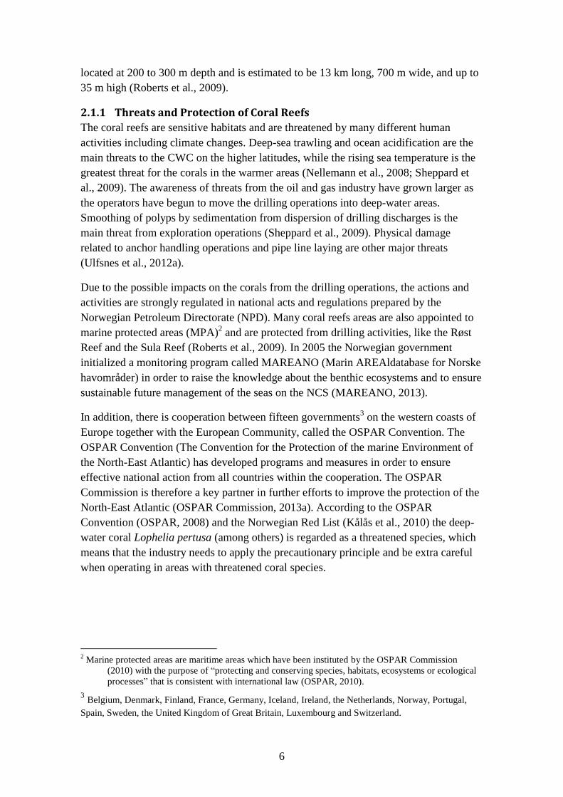
2.1.1 Threats and Protection of Coral Reefs

The coral reefs are sensitive habitats and are threatened by many different human

activities including climate changes. Deep-sea trawling and ocean acidification are the

main threats to the CWC on the higher latitudes, while the rising sea temperature is the

greatest threat for the corals in the warmer areas (Nellemann et al., 2008; Sheppard et

al., 2009). The awareness of threats from the oil and gas industry have grown larger as

the operators have begun to move the drilling operations into deep-water areas.

Smoothing of polyps by sedimentation from dispersion of drilling discharges is the

main threat from exploration operations (Sheppard et al., 2009). Physical damage

related to anchor handling operations and pipe line laying are other major threats

(Ulfsnes et al., 2012a).

Due to the possible impacts on the corals from the drilling operations, the actions and

activities are strongly regulated in national acts and regulations prepared by the

Norwegian Petroleum Directorate (NPD). Many coral reefs areas are also appointed to

marine protected areas (MPA)2 and are protected from drilling activities, like the Røst

Reef and the Sula Reef (Roberts et al., 2009). In 2005 the Norwegian government

initialized a monitoring program called MAREANO (Marin AREAldatabase for Norske

havområder) in order to raise the knowledge about the benthic ecosystems and to ensure

sustainable future management of the seas on the NCS (MAREANO, 2013).

In addition, there is cooperation between fifteen governments3 on the western coasts of

Europe together with the European Community, called the OSPAR Convention. The

OSPAR Convention (The Convention for the Protection of the marine Environment of

the North-East Atlantic) has developed programs and measures in order to ensure

effective national action from all countries within the cooperation. The OSPAR

Commission is therefore a key partner in further efforts to improve the protection of the

North-East Atlantic (OSPAR Commission, 2013a). According to the OSPAR

Convention (OSPAR, 2008) and the Norwegian Red List (Kålås et al., 2010) the deep-

water coral Lophelia pertusa (among others) is regarded as a threatened species, which

means that the industry needs to apply the precautionary principle and be extra careful

when operating in areas with threatened coral species.

2 Marine protected areas are maritime areas which have been instituted by the OSPAR Commission

(2010) with the purpose of “protecting and conserving species, habitats, ecosystems or ecological

processes” that is consistent with international law (OSPAR, 2010).

3 Belgium, Denmark, Finland, France, Germany, Iceland, Ireland, the Netherlands, Norway, Portugal,

Spain, Sweden, the United Kingdom of Great Britain, Luxembourg and Switzerland.

7

2.2 PETROLEUM AND DRILLING OPERATIONS ON THE NORWEGIAN

CONTINENTAL SHELF

Petroleum, oil and natural gas, is formed from deposed organic matter in the oceans that

has been decomposed and converted into hydrocarbons over several millions of years.

The hydrocarbons are developed in a rock called the source rock (Figure 3). Depending

on pressure and the rock’s permeability, the oil and gas may seep out of the source rock

and migrate through porous water-bearing rocks. This migration can take place because

the hydrocarbons are lighter than water and continue over thousands of years and extend

over tens of kilometres until it is stopped by a denser layer (Figure 3). The dense layer

is usually shale or mudstone and need to have a shape that can trap the oil in order to

provide a reservoir of oil and gas. The reservoir rock, which contains the petroleum, is a

porous rock, usually sand or limestone, and contains saturated compositions of water,

oil and gas (MPE & NPD, 2012; Lyngrot, 2013).

Figure 3: Illustration of developing process of an oil and gas reservoir (Lyngrot, 2013).

In 1963, the Norwegian government claimed the NCS after a requested permission for

exploration drilling with the intention to acquire exclusive rights, and stipulated that the

Norwegian state was the landowner of the whole shelf (MPE & NPD, 2012). The shelf

became divided into several blocks representing specific and defined geographical areas

(Ministry of Petroleum and Energy, 2013a). Before oil companies are allowed to start

explore a block they need a license from the authorities. The first licensing round was

announced on the 13 of April 1965, which covered 78 blocks and 22 production licenses

were awarded.

The most promising blocks have been announced first for each licensing round, as is the

reason for world-class discoveries on the NCS (MPE & NPD, 2012). The first

exploration well in which oil was discovered in Norway was at Ekofisk in 1969 and the

production started there in 1971. Today, there are about 50 active companies, both

8

Norwegian and foreign, operating on the NCS. Figure 4 gives an overview of the area

status on the NCS in March 2012 made by the Norwegian Petroleum Directory (NPD;

MPE & NPD, 2012).

Figure 4: Area status of petroleum activity on the Norwegian continental shelf in March 2012

(MPE & NPD, 2012).

2.2.1 Petroleum Regulations and Licensing Process

A governmental approval and permit are required in all phases of the petroleum

operations on the NCS. The general legal basis for the licensing system is provided by

the Petroleum Act (Act 29 November 1996 No. 72; Ministry of Petroleum and Energy,

2013a) and together with the Regulations of the Act (Regulations 27 June 1997 No. 653;

Ministry of Petroleum and Energy, 2013b). There are two types of licensing processes

in Norway. The regular licensing round held every second year since the beginning in

9

1965 and a new form of licensing round system which entails award of production

licenses in predefined areas (APA) started in 2003. This new licensing round is a

regular, fixed cycle and has been held every year since the start (MPE & NPD, 2012).

The oil companies apply for licenses individually or as part of a group. A license can

comprise parts of a block, an entire block or multiple blocks. The applicants’ technical

expertise, understanding of geology, financial strength and experience are considered by

the authorities when awarding the licenses (NPD, 2008). The applicants first get a

license for an initial-period of exploration in four to six years, which can be extended

for up to ten years. After completing the initial period, and if the area has proven to

contain oil and gas, the company can apply for an extension of the license to a

production license, which in general lasts for 30 years. If oil and gas are not found in the

area the area shall be relinquished (NPD, 2008).

Besides the Petroleum Act and the Regulation of the Petroleum Act, the petroleum

industry in Norway is regulated in the Activities Regulation. This regulation covers all

activities related to the petroleum industry from emergency preparedness to allowed

emission and discharge levels to the external environment (PSA, 2013). To prevent

damage on the vulnerable environmental resources from the petroleum industry, the

Activities Regulation requires environmental monitoring and the requirements for this

actions must be met before, during and after the conducting of the drilling activities

(PSA, 2013). The monitoring is further regulated in the Guidelines for environmental

monitoring of the petroleum activities on the Norwegian continental shelf (KLif, 2009).

Moreover, the Pollution Control Act also requires the polluter to monitor the

environmental impact of its operations (MD, 1981).

2.2.2 The Drill Planning Process

During the initial licensing period the applicant gets a specific work commitment

including activities such as seismic data acquisition, surveys and/or exploration drilling

(NPD, 2008). The exploration-wells are drilled in order to investigate the area further

and to investigate whether the predicted reservoir contains any oil and gas. However,

before the drilling operation can begin, a drill program must be set. In this drill planning

process, all drilling activities, such as dispersion of drilling discharges, anchor and

mooring chain installation, recovery operations and deployment of necessary

infrastructure, must be considered in order to make the drilling operation both safe and

efficient, and to reduce the risk of negative impact in sensitive areas (Lyngrot, 2013).

An essential part of the planning process from an environmental point of view, is to

perform a monitoring program and to identify sensitive and vulnerable areas/species

that need to be taken into consideration (Figure 5). In order to develop a monitoring

program that focuses on those areas that may be at risk, it is recommended to perform

an impact assessment in order to get an overall risk picture (Ulfsnes et al., 2012a). The

pre-study and the site survey, which are mandatory activities in the work commitment,

provide necessary data to the impact assessment.

10

Figure 5: General process and actions involved in the drill planning process of a drilling

operation from an environmental point of view (DNV, 2013)

In the impact assessment, a risk assessment is most often included. The risk assessment

helps to evaluate the risks inflicted upon the sensitive areas and is used as a decision

support for operators when planning the drilling operation and performing the

monitoring program. Det Norske Veritas (DNV) has developed a specific risk

assessment method called Coral Risk Assessment (CRA), where they combine mapping

of the resources with modelled simulations of the discharges (Ulfsnes et al., 2012a). The

CRA analysis is presented in chapter 2.3.1.

2.2.3 Exploration Drilling

The well planning process and development of a drilling program, is a large and

important part of the whole exploration process to make the drilling operation safe and

efficient. The pre-study and site survey provide information that is used in order to

pinpoint the reservoir and determine the drilling path for the exploration drilling.

The drilling operation is done in sections (Figure 6). Generally, a 36” hole is first drilled

in the seafloor, the top hole. In the top hole, a 30” conductor is placed. The conductor

provides an initial stable structural foundation for the borehole and the well, and isolates

unstable near-surface soil. The next sections are drilled in different sizes and numbers

depending on the formation in the wellbore, where unconsolidated rocks, permeable

rocks and the formation pressure/pore pressure are taken into account. In every drilled

section, a casing is placed. A casing is a steel tube designed to prevent the formation

from caving in, formation fluids from entering the wellbore and drilling fluid from

11

being lost to the formation. The casing needs

to be cemented in place to serve its purpose.

The cementing anchors the casing and isolates

the well from high pressures (Lyngrot, 2013).

In the last section drilled above the reservoir, a

special production casing is normally

installed.

The final section is drilled through the

reservoir. In this section, a casing called liner

is cemented in place. In contrast to the other

casings the liner is only extended into the

production casing and does not go all the way

up to the surface. Essential for the liner is an

adequate cementing and isolation to the

production casing, which creates a pressure

barrier and provides production from selected

zones in the reservoir trough the liner. During

the drilling of the last section, important data

are collected by logging in the hole and by

core sampling from the rock (Lyngrot, 2013).

While drilling the well, drilling fluid or drilling mud is used. The function of the drilling

fluid is to lift up cuttings from the borehole to the surface, stabilize the wellbore by

providing hydrostatic pressure, cool down the drill bit and lubricate the drill string

(Lyngrot, 2013). The drilling fluid needs to have the right properties in terms of

viscosity, gel strength, density and filtration rate to be able to have these functions.

The most important function is to provide hydrostatic pressure, which is obtained when

the pressure of the drilling fluid lies between the pore pressure and the fracture

pressure4. If the pressure exceeds the fracture pressure the wellbore can break down and

provide stability problems around the drill bit. Extensive pressure can also lead to well

control issues where fluid can be lost to the formation or dynamic over/under pressure

can occur. The window between pore pressure and fracture pressure is often narrow,

making the drilling challenging. In other words different drilling fluids are used in

different drilling section to obtain a stable hydrostatic pressure. In deeper sections

heavier fluids are used and the casing in the upper sections stabilizes the wellbore from

being affected by these heavier fluids (Lyngrot, 2013).

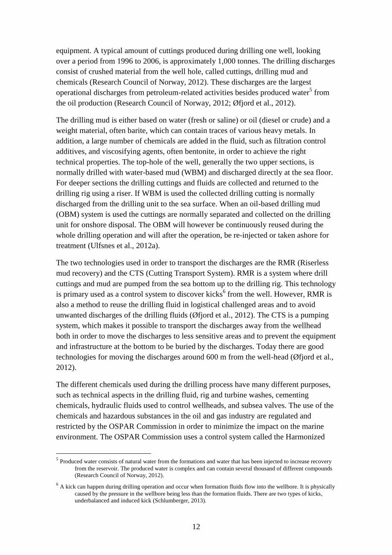
2.2.4 Drilling Discharges

During the drilling process a large amount of discharges are produced from the drilling

operation, including cementing, maintenance and testing operations on the drilling

4 The pore pressure refers to the pressure of the fluid within the formation. The fracture pressure is the

pressure above which injections of fluids cause on the rock formation to fracture hydraulically

(Lyngrot, 2013).

Figure 6: Schematic overview of a

general drilling process with sections,

casings and the liner (Lyngrot, 2013).

12

equipment. A typical amount of cuttings produced during drilling one well, looking

over a period from 1996 to 2006, is approximately 1,000 tonnes. The drilling discharges

consist of crushed material from the well hole, called cuttings, drilling mud and

chemicals (Research Council of Norway, 2012). These discharges are the largest

operational discharges from petroleum-related activities besides produced water5 from

the oil production (Research Council of Norway, 2012; Øfjord et al., 2012).

The drilling mud is either based on water (fresh or saline) or oil (diesel or crude) and a

weight material, often barite, which can contain traces of various heavy metals. In

addition, a large number of chemicals are added in the fluid, such as filtration control

additives, and viscosifying agents, often bentonite, in order to achieve the right

technical properties. The top-hole of the well, generally the two upper sections, is

normally drilled with water-based mud (WBM) and discharged directly at the sea floor.

For deeper sections the drilling cuttings and fluids are collected and returned to the

drilling rig using a riser. If WBM is used the collected drilling cutting is normally

discharged from the drilling unit to the sea surface. When an oil-based drilling mud

(OBM) system is used the cuttings are normally separated and collected on the drilling

unit for onshore disposal. The OBM will however be continuously reused during the

whole drilling operation and will after the operation, be re-injected or taken ashore for

treatment (Ulfsnes et al., 2012a).

The two technologies used in order to transport the discharges are the RMR (Riserless

mud recovery) and the CTS (Cutting Transport System). RMR is a system where drill

cuttings and mud are pumped from the sea bottom up to the drilling rig. This technology

is primary used as a control system to discover kicks6 from the well. However, RMR is

also a method to reuse the drilling fluid in logistical challenged areas and to avoid

unwanted discharges of the drilling fluids (Øfjord et al., 2012). The CTS is a pumping

system, which makes it possible to transport the discharges away from the wellhead

both in order to move the discharges to less sensitive areas and to prevent the equipment

and infrastructure at the bottom to be buried by the discharges. Today there are good

technologies for moving the discharges around 600 m from the well-head (Øfjord et al.,

2012).

The different chemicals used during the drilling process have many different purposes,

such as technical aspects in the drilling fluid, rig and turbine washes, cementing

chemicals, hydraulic fluids used to control wellheads, and subsea valves. The use of the

chemicals and hazardous substances in the oil and gas industry are regulated and

restricted by the OSPAR Commission in order to minimize the impact on the marine

environment. The OSPAR Commission uses a control system called the Harmonized

5 Produced water consists of natural water from the formations and water that has been injected to increase recovery

from the reservoir. The produced water is complex and can contain several thousand of different compounds

(Research Council of Norway, 2012).

6 A kick can happen during drilling operation and occur when formation fluids flow into the wellbore. It is physically

caused by the pressure in the wellbore being less than the formation fluids. There are two types of kicks,

underbalanced and induced kick (Schlumberger, 2013).

13

Mandatory Control System, which encourages the use of less or non-hazardous

substances (OSPAR Commission, 2013b).

Figure 7: A flow chart on how to perform safe drilling operations and to get discharge permit

for drilling discharges in waters with presence of cold water corals (Ulfsnes et al., 2012a).

Until 1993, the most important source of operational oil discharges was from the

petroleum industry. Substantial amount of cuttings, also containing oil, were discharges

together with residues of both WBM and OBM. This led to regulations for discharges of

cuttings and cuttings containing more than 1% oil were prohibited. In practice,

operational discharges today only take place from drilling operations using WBM

(Research Council of Norway, 2012) and discharge permission is mandatory before the

drilling companies are allowed to discharge any drill cuttings or drilling fluids. A

typical scenario in the drill planning process on how to perform safe drilling operations

and discharges in waters with presence of CWC is given in a flowchart in Figure 7

(Ulfsnes et al., 2012a).

14

2.2.5 Behaviour of Drilling Discharges

To understand the environmental risks associated with dispersion of drilling discharges,

knowledge about the behaviour of the discharge in the oceans is important (Figure 8).

The path of the discharge is decided by the ocean currents velocities and direction, and

the stratification in the water column, which is set by the vertical variation of salinity

and temperature. When the density of the descending plume and the ambient water is

equal the discharges will start to sink (Rye et al., 2006). Depending on the different

properties of the particles, the sinking velocities will be different. The size is the most

important attribute to decide the behaviour of the particle in the water column.

However, the whole composition of the drilling discharges will affect the behaviour and

sinking velocities of the particles (Vanoni, 2006).

Figure 8: Illustration of the processes involved in the water column and at the seabed, when

drilling discharges are released into the sea (Rye et al., 2006).

The sinking velocities of a spherical particle can be described with Stoke’s Law. For a

sphere of diameter d, the fall velocity w, for values of Reynolds number, ⁄ ,

less than approximately 0.1, the sinking velocity is given by:

(

) ( )

where is the kinematic viscosity, is the specific weight of the fluid, g denotes the

acceleration of gravity, and is the specific weight of the sphere (Vanoni, 2006, p. 14).

Natural particles are usually asymmetric and generally have a lower sinking velocity.

However, even if the velocity cannot be calculated directly from Stoke’s Law the

15

application of the equation is done nevertheless. The sinking velocity of larger particles

is mostly dominated by friction (Vanoni, 2006).

As discussed by Rye et al. (2006), the drilling discharges will contribute to risks or

stressors for the sensitive fauna, in both the water column and the sediment (Figure 8).

Generally, there are two types of stressors in the water column and four in the sediment.

The drill cuttings and mud will result in increased concentrations of suspended particle

matter (SPM) in the water column that will cause a physical stress (not toxicity) on the

organism living in the water column. Larger particles will not contribute to the risk thus

they will tend to descend to the sea floor (Rye et al., 2006). The second stressor in the

water column is the impact from chemicals that are assumed to be dissolved. Chemicals

with partition coefficient Pow7 < 1000 L/kg are assumed to be dissolved completely.

Chemicals with a larger partition coefficient are deposed on the sea floor, due to a large

ability to be absorbed by organic matter or have properties that force the particles to

agglomerate (Rye et al., 2006).

The sediment stressors come from the deposit of drilling discharges. The deposit will

cause a new sediment layer of cuttings and mud, a change in grain size and the toxicity

caused by the attached chemicals, including heavy metals (Rye et al., 2006). After the

deposition on the sea floor, natural processes will start to recover the sea bed. These

main processes are dilution effects due to burial of natural deposition after the

discharge, bioturbation by benthic organisms in the sediment, which mix the particles

vertically and cause a distribution of the median grain size, the biodegradation of

chemicals and re-suspension of deposited matter. The biodegradation of chemicals will

cause the sixth stressor, due to oxygen depletion in the sediment (Rye et al., 2006).

2.2.6 Environmental Impact from Drilling Discharges

An environmental improvement on the Norwegian continental shelf has been shown by

monitoring activities since it only became permitted to discharge cuttings from water-

based mud. However, it is still uncertain if the added substances, even if they primarily

are PLONOR (Pose Little or No Risk to the environment) or are considered as non-

hazardous chemicals, can have undesirable effects over a long period (Research Council

of Norway, 2012). In other words, the behaviour of the drilling discharges in both the

water column and the sediment must be studied to understand the total risk of drilling

operations for the environment.

PROOFNY, a program founded by Norwegian Oil Industry Association (Norwegian oil

and gas), Ministry of Petroleum and Energy (MPE) and Ministry of the Environment

(MD), have done research in order to increase the knowledge, and investigate the long-

term effects of discharges from petroleum-related activities. In some of the projects the

long-term effects of water-based drilling discharges have been specifically investigated

(Research Council of Norway, 2012). The experiments in these projects showed a

reduction of certain sensitive animal species in the sediment (no species disappeared

7 Pow is partition coefficient determined from the HOCNF testing procedure.

16

completely) and a weak effect on recruitment to benthic fauna. The main reason for

these biological effects is believed to be the reduction in oxygen due to biodegradation

of the chemicals in the sediment. However, there was also an indication that toxicity

could have acted as a contributing factor. Smothering by sedimentation from the drilling

discharges, and the form and size of the cutting particles showed to have an effect if the

layer of cutting were >10 mm, which normally is the case within a distance shorter than

250 m from the release location (Research Council of Norway, 2012).

Additional effects in the water column were noted in further research in the PROOFNY

framework on bioavailability of heavy metals in the weight materials (barite) in the

drilling mud. This research indicated that the effects from the drilling fluid are mostly

due to physical stress and not metal toxicity. However, the experiments did not say

anything about how quickly the metals are absorbed, just that they are bioavailable. The

physical stress comes from the suspended particles, which probably only will have a

local and short-lived effects on the animals in the water masses. Hence, the cumulative

effects in the water column are unlikely to occur, since the same water mass will

probably not be exposed to repeated discharges of drill cuttings and mud (Research

Council of Norway, 2012).

More specific studies on how Lophelia pertusa reacts on discharges from drilling

activities have been done in laboratory experiments by Larsson and Purser (2011). The

experiments showed that sediment load and duration of the discharge are the most

important factors for coenosarc loss (loss of skin) and mortality (Table 1; Ulfsnes et al.,

2012a).

Table 1: Findings from experiments on the long term effects by sedimentation on Lophelia

pertusa done by Larsson and Purser (2011).

Physical impact Experiment results

Sediment coverage Only related to duration of discharge, not sediment load or the combination of load and duration.

Coenocarc loss The proportion of coral fragments that lost coenosarc was significantly affected by sediment load.

Mortality Increased with sediment load (0.5% and 3.7% at exposure levels of 6.5 and 19 mm respectively over a period of 21 days).

Growth In a time scale of 21 days the growth was not affected.

2.3 RISK MANAGEMENT

The effect of uncertainty of the result for a given action or activity can be described as a

risk, either positive or negative. The main process of managing risks is to perform a risk

assessment. The risk assessment is done in three steps; risk identification, risk analysis

and risk evaluation. The purpose of the risk assessment is to provide evidence-based

information, to make decisions on how to treat a particular risk and select between

options. The risk assessment tries to answer fundamental questions like; What can

happen and why? What are the consequences? What is the probability of the future

occurrence? And are there factors changing the consequence or reducing the probability

17

of the risk? (ISO, 2009). A risk-based approach is preferable for manage the

environmental risk associated with drilling operations offshore and to protect and

minimise the chance of negative effect on vulnerable species.

2.3.1 Coral Risk Assessment (CRA)

The CRA analysis is a risk assessment method developed by Det Norske Veritas

(DNV). CRA is a method that evaluates the risk inflicted upon the cold water corals

(CWC) in exploration areas in order to help operators to plan an exploration drilling

with the lowest possible risk for the corals. When an overall risk assessment for the

CWC is made, it is also easier to develop a monitoring program focusing on those coral

structures that may be at risk. This method can likewise be used for other sensitive

fauna, such as sponges (Ulfsnes et al., 2012a).

Table 2: Required background data and input parameters to perform the coral risk assessment

(Ulfsnes et al., 2012a).

Data Optional/ Mandatory Description

Drilling plan Mandatory A plan over the drilling operation. Describing volumes of expected discharges of cuttings and mud, duration of drilling operations, discharge location etc.

Map over potential coral structures

Mandatory Maps based on sonar data were potential coral structures are pinpointed.

Coral survey data Optional Confirmation data on the presence of corals, coral condition, coral species and distribution. These data make it possible to distinguish coral structures which will strengthen the risk assessment.

Current data Optional Important data to be able to assess the current regime at a given location, which is important with regards to spreading of the discharge.

Modelled dispersion plume

Optional Gives an overview of the dispersion and sedimentation rate. Essential when assessing possible impacts inflicted upon CWC. Should be based on site specific measurements.

Anchor analysis Mandatory Location of anchor, anchor chains, pennant wires etc.

The CRA analysis is based on different background data, collected during the drill

planning process, and input parameters (Table 2). Important background data are

information about the drilling operation and a resource map showing potential coral

structures. To be able to make a better judgement of the risk inflicted upon the CWC,

data that confirm presence of the coral structures are preferable, together with site

specific current data and a modelled dispersion plume (Ulfsnes et al., 2012a). The risk

assessment can also include an anchor analysis in which a best fit analysis for the

locations of the anchor is made, with regards to the presence of coral targets in the

operation area.

18

The mapping of possible coral structures at the sea floor is most commonly done during

the site survey with a side scan sonar (SSS) or and multi-beam echo sounder (MBES).

The typical size of the area these methods cover is 4x4 km. From the sonar mapping

potential coral structures can be detected. To confirm and identify the condition of the

coral structures a visual mapping with an ROV (Remotely Operated Vehicle) is

recommended. The condition and distribution of the coral species are identified and

verified during the visual mapping. Also, other important findings can be detected such

as effects from trawling and other vulnerable species (Ulfsnes et al., 2012a). The

techniques and methods are given in NS9435, which is a Norwegian standard describing

methods and equipment for visual collecting of environmental data from the sea

(Standard Norge, 2009).

Table 3: Coral condition criteria in the CRA analysis (Ulfsnes et al., 2012a).

Lophelia condition Coral garden

Area of living Lophelia pertusa (m2)

Coverage (% of living corals)

Specimens per 25m2

Poor < 15 0 - 20 < 5

Fair 15 - 50 20 - 40 5 - 10

Good 50 - 100 40 - 60 10 - 15

Excellent > 100 > 60 > 15

Based on the ROV data a rough estimation of habitats is calculated for each potential

coral area identified within the SSS mosaic. The habitats are given as a percentage of

the area, usually divided into four criteria groups (Table 3) (Ulfsnes et al., 2012a). Also

coral gardens can be included in the categorization. When the corals have been

categorized, a consequence analysis is made based on expected sedimentation and the

condition of the coral structure. The modelled plume gives an overview of the

dispersion and the sedimentation rates based on the expected drilling discharges and the

current data (Ulfsnes et al., 2012b).

Table 4: Consequence matrix based on expected sedimentation of drill cuttings and mud and

condition of coral structure (Ulfsnes et al., 2012a).

Degree of exposure

Lophelia Pertusa condition

Poor Fair Good Excellent

Negligible (0.1 - 1 mm) Minor Minor Minor Minor

Low (1 - 3 mm) Minor Moderate Moderate Moderate

Significant (3 - 10 mm) Minor Moderate Serious Serious

Considerable ( > 10 mm) Minor Serious Severe Severe

In general the categorizations of consequence are a function of distance from discharge

location and condition of the coral structure. At larger distance sedimentation of drilling

discharges is less than closer to the discharge location and the consequences for coral

structures in good condition are considered to be larger than for coral structures in poor

19

conditions (Ulfsnes et al., 2012b). The consequence scale is divided into four groups;

minor, moderate, serious and severe, and the exposure degree of sedimentation is

divided into four groups (Table 4; Ulfsnes et al., 2012a). The criteria, for each

consequence group divided in sedimentation levels, are generated from threshold values

for burial of Lophelia pertusa. The threshold values worked out are based on the

laboratory experiments done by Larsson and Purser (2011).

Table 5: Description of the probability scale of corals being covered by sedimentation from

discharges of drill cuttings and mud (Ulfsnes et al., 2012a).

Probability Description

Expected Expected during an operation of this type

Likely May be expected during an operation of this type

Rare May occur but not to be expected during an operation of this type

Unlikely Possible but with very low probability

The risk inflicted upon the coral targets, is assessed by combining the consequence and

the probability for the corals to be affected by the drilling discharges. The dispersant

plume varies with current speed and direction and can be seen as an expression of

probability. The probability scale is therefore generated from the current measurements.

By dividing the current values into different datasets using the geographical information

systems software ArcGIS, the datasets are generating diagrams of current magnitude

and directions around the well location. These diagrams are laid above each other

generating isolines of probability that are fit into the sedimentation area. The isolines

are divided into four groups based on the probability for sedimentation or spread of drill

cuttings and mud (Table 5; Ulfsnes et al., 2012b).

Table 6: Risk matrix based on the probability- and consequences scale for the corals to be

affected by the drilling discharges (Ulfsnes et al., 2012a).

Probability

Consequence

Minor Moderate Serious Severe

Unlikely Rare Likely Expected

To perform the final risk assessment matrix the probability scale is combined with the

consequence matrix (Table 6; Ulfsnes et al., 2012b). From the risk matrix the discharge

location can be evaluated if the risk of the corals being affected by the operations is too

high or low enough. The decision about need of action in order to minimise the risk for

the coral targets in the drilling area, should be based on both authorities’ and the

operators’ environmental policies and guidelines.

20

2.4 CASE OF STUDY – THE PUMBAA FIELD

During November and December, 2009, an exploration well at the Pumbaa Field

(NOCS 6407/12-2) in the Norwegian Sea was drilled (Figure 9). The well was drilled in

block 6407/12 and in production license PL 469. The exploration-well is located at

64.16 degrees latitude and 7.8 degrees longitude, about 57 km north-east from Frøya

and about 10 km south from the Draugen field, and at a depth of 307 m. The marine

protected area, the Sula reef, is located about 10 km west of the drilling location

(Ulfsnes et al., 2010). The company responsible for the drilling activities was GDF

SUEZ E&P Norge AS. The drilling was done with a new semi-submersible drilling rig

called Aker Barents and was operated by Aker Drilling ASA (Aaserød et al., 2009). The

analysis in this study concerns this drilled exploration-well.

Figure 9: Map over the position of the exploration well Pumbaa (PL 469) on the Norwegian

Continental Shelf.

2.4.1 Drill planning process

An early phase study on the environmental resources in the area around block 6407/12

was made beside the site survey in order to find vulnerable areas and species that may

be at risk for an acute oil spill and needed to be taken into consideration while planning

the drilling operation. In the study, which was made form an on-going work with an

21

integrated management plan for the hole Norwegian sea, the bottom resources (benthic

fauna) were investigated together with fishery resources, sea birds, marine mammals

and shore/protected areas, fishing and aquaculture (Aaserød et al., 2009). In the site

survey several areas of corals were identified south and southeast of the drilling

location, with the closest located approximately 280 m from the well location. An area

of 4x4 km in total was studied with the use of SSS/MBES and some of the corals were

located on seabed mounds/ridges that showed accumulative heights of up to 12.5 m.

The coral species found in the site survey was Lophelia pertusa and Paragoria arborea

(Furgo Survey AS, 2008).

Due to the coral targets being close to the drilling location the risk reduction suggested

for the drilling activities was to move the discharge location using CTS technology or

collecting the drill cuttings and mud at the rig using a riser, and bring it to shore for

treatment. In either case monitoring of the effect on corals was recommended (Aaserød

et al., 2009).

2.4.2 The Monitoring Program

The monitoring activities were carried out by DNV during three cruises; first, to collect

baseline data before the drilling started, second, to monitor during the drilling activities

and last, to monitor the actual effect from the drilling operation.

Table 7: Measurements performed during the monitoring program before, during and after the

drilling operation at Pumbaa (Ulfsnes et al., 2010).

Parameter Sampling

Methodology Deliverables Before During After Ref.

Current Yes Yes Yes - Quantitative Current conditions at 2 and 10 m above sea floor

Turbidity Yes Yes Yes Yes Semi- Quantitative

Turbidity in the water masses at 2 and 10 m above the sea floor. Before/after - control/impact.

Grain size and heavy metals in sediment

Yes Yes Yes Yes Quantitative Before/after - Control/impact analysed from core-sample taken from of all sediment stations

Drill cuttings thickness

NA Yes Yes Yes Descriptive Estimation of drill cutting thickness analysed from core-sample taken from all sediment stations.

Drill cuttings distribution

NA Yes Yes - Descriptive Estimation of drill cutting distribution from the ROV surveys.

Effects on corals

Yes Yes Yes - Descriptive Evaluation of video material from ROV surveys.

22

In the monitoring program the main task was to monitor the dispersion of drilling

discharges in the water column and to assess effects from drilling activities on the coral

communities in the area. In order to quantify the impact from the drilling activities on

the coral structures the monitoring program included collection of data showing current

movements and sedimentation patterns (Table 7). Information of the sedimentation

patterns was collected by turbidity measurements, sediment traps in the water column

and sediment sampling from the seafloor. The sediment traps were analysed for heavy

metal and dry weight and the sediment samples for heavy metal and granulometry

(grain size). Turbidity and current measures were also done at the Sula reef (Ulfsnes et

al., 2010).

In August 2009, during the baseline data cruise, a further monitoring was done to

determine the existence and extent of coral structure. The investigation resulted in six

potential coral structures of Lophelia, with the closest structure situated 300 m south of

the drilling location (Table 8). One solitary colony with Paragogia arborea was

identified (Ulfsnes et al., 2010).

Table 8: Information regarding the six coral targets found in the monitoring survey done with

the ROV before in the exploration drilling area at Pumbaa (Ulfsnes et al., 2010).

Target Distances and bearing

from the discharge location

Distance and bearing from the drilling

location Height

L. pertusa condition

1 622m 165° 343m 179° 6m Poor

2 636m 153° 337m 155° 0.5m No living

3 582m 201° 459m 232° 1m Fair

4 761m 194° 582m 214° 2.5m Fair

5 554m 173° 300m 195° 1.8m Poor

6 631m 195° 471m 222° 3.5m Fair/Poor

P. arborea 295m 275° 534m 304° 0.5m -

2.4.3 Important findings from the monitoring program at the Pumbaa field

The turbidity was measured at six locations at 2 and 10 m above the sea floor (Marked

T in Figure 10). The turbidity was measured in FTU (Formazine Turbidity Units) which

gives a relative measure of the permeability of the water to UV rays in the instrument.

The FTU is typically increased in response to an increase in SPM. The measured

turbidity showed that the FTU values in general were low, ranging from 0.34 to 2.35

FTU (Ulfsnes et al., 2010).

The sediment was analysed from both sediment traps in the water column (before and

during/after drilling) and from seabed samples at five stations before and at 20 stations

after drilling (Figure 10). The analysis of the dry weight from the sediment traps

showed that the measures at TS2 had an increase of 400% of collected sediment. TS2 is

located 100 m from the discharge location and the increase is most likely from the

drilling activity (Ulfsnes et al., 2010). The heavy metal concentration was also analysed

23

in the sediment traps. The data set showed a significant increase in trend of barium

cncentration, 103 mg/kg, before drilling and 2,959 mg/kg during/after drilling (Ulfsnes

et al., 2010). The highest concentration was observed at TS1 and the lowest at TS2. TS2

is the closest location to the discharge location and because of the highest sediment

value the explanation is most likely that the barium level has been diluted from the drill

cuttings. Drill cuttings have a high affinity to metals and the finer sediments have

probably drifted further away before they have settled down (Ulfsnes et al., 2010).

Figure 10: Detailed map over the monitoring activities. The grey area shows the ROV activities

done before the drilling operation in order to do a visual investigation of the coral targets.

Monitoring rigs are marked with “X”, sediment stations with and coral target with . All

Sediment stations were sampled after the drilling campaign. The sediment stations marked with

“b” were also sampled before the drilling campaign (Ulfsnes et al., 2010).

The analyses of metals in the sediment samples showed a significant change of barium

between samples before and after drilling. The average barium concentration increased

by a factor of five and the maximum concentration was registered at the closest sample

to the discharge location. An interpolation using the kriging method was done with the

24

concentration of barium from after the drilling and compared with the LSC (Level of

Significant Contamination) of 193 mg/kg barium, which has been calculated for the

Haltenbank region on the NCS (Figure 11). The interpolation showed that an estimated

area of 158,000 m2 had barium levels above the LSC level after the drilling campaign.

This reached a radius of approximately 250 m from the discharge location (Ulfsnes et

al., 2010).

Figure 11: Contour map showing levels of barium after the drilling campaign at Pumbaa. An

interpolation with the kriging method has been done based on the sample locations ( ). The

maximum registred concentration was added to the discharge location assuming this has at least

the same barium level. The green dots represent the location of coral targets (Ulfsnes et al.,

2010).

25

The current direction and speed were measured at one location during four months, at 2

and 10 m above the sea floor (Marked TC4 in Figure 10). The current direction gives an

indication of the spread of drilling discharges and is an important indicator of possible

effects on the coral structures. An analysis of the current direction shows that the

current during drilling the 36” section contributed the most to transport of cutting

towards the coral structures (Figure 12) (Ulfsnes et al., 2010).

Figure 12: Current velocities and directions at 2 and 10 m above the seafloor during the time of

drilling the three sections (36”, 8½” and 17½”) at the CTS loaction. Speed and direction: Blue

<10 cm/s, Yellow 10-20 cm/s, Green 20-30 cm/s (Ulfsnes et al., 2010).

During the visual survey with the ROV, during the discharge period, a pile of cuttings

about 1 m high was observed at the discharge location. During the survey after the

drilling operation a pile about 0.5 m high was observed approximately 60 m south west

of the discharge location. From this pile, deposited drill cuttings were observed 70 m

west and 40 m south east. Areas further away along the survey line had no indications

of deposited material, which limited the radius of significant spread of drilling

discharges to <100 m from the discharge location (Ulfsnes et al., 2010).

A comparison of model simulations to field data from the monitoring program of the

Pumbaa field has been carried out by Rye et al. (2012). The comparison was made with

model simulations for the actual drilling discharges and with field data, from the

turbidity measurements and the barium concentration in the sediments. Rye et al. (2012)

found a good correspondence in time between concentration peaks 2 m above the sea

floor simulated by the model and the occurrences of the turbidity peaks measured at

26

TS2, TS3 and TS5. Regarding the simulated concentrations, they seem to be an order of

magnitude larger than the measured turbidity.

The actual barium concentration in the sediment was compared with the simulated

spread of barite (BaSO4) by the model. The barite concentrations for the 20 sediment

locations were converted to barium content in the upper centimetres of the sediment and

corrected for background values. The overall results showed, again, one magnitude too

large value of simulated barium increase in the sediment, compared with the measured

increase of barium at the end of the discharge period. The averaged value of increased

barium in the surface sediment for all the 20 locations was 6.13 g/m2 based on measured

values. The same simulated value of average barium content was 92.84 g/m2. These

results are believed depend on the pile that builds up at the hose of the CTS preventing

the particles from spread outside the crater. Rye et al. (2012) referred to this

phenomenon as the “crater effect” and stated that simulations with the DREAM model

overestimated the spread of drilling discharges by factor of 15.

27

3 METHOD The overall goal of this study is to compare and evaluate simulations from two different

models, the DREAM model (Version 6.2) and the MUDFATE model, for the

exploration-well (PL 469) drilled on the Pumbaa field in November 2009 on the

Norwegian continental shelf (NCS). The modelling with the MUDFATE model is made

by the Computational Hydraulic and Transport (CHT). The study will hopefully bring

insight into how to perform dispersion modelling in an appropriate way in order to

improve the risk assessment method and make better judgement on how the corals will

be affected from drilling operations on the NCS.

The analysis method consists of two main parts. The first part is to model the dispersion

of drilling discharges for the drilling operation at Pumbaa. These simulations will be

done for the planned drilling discharges of the drilling operation and for the drilling

discharges from the actual drilling operation. The results from the modelling will be

compared to monitoring data from the monitoring program in order to evaluate how

well the models manage to simulate the actual spread of the drilling discharges.

The second part is to perform the CRA analysis for both the planning phase and the

actual drilling phase. The CRA analysis is done in order to determine differences in the

risk picture for the coral targets in the area between using different types of parameters

in the dispersion modelling and how well these parameters simulate the actual spread of

the drilling discharges in the area. The CRA analysis will also try to evaluate whether

the decision to move the release site was a good decision in order to reduce the risk for

the coral targets from being affected by the drilling discharges.

3.1 DISPERSION MODELS

When performing risk assessments, an important step is to determine the consequences

and probability of an event to occur. This is most often determined by modelling an

outcome of an event or a set of events (ISO, 2009). Depending on the type of event, the

model has to manage different features and be designed accordingly in order to provide

adequate results. However, essential for all models is that the input data are accurate for

the actual event to provide adequate results. Models handling drilling discharges have to

manage features such as

That the duration of drilling discharges is generally short.

That discharges of cutting and mud contain large amount of mineral particles.

That the discharges may cause deposits on the sea floor.

The behaviour of the discharge in both the water column and in the sediment is

therefore an important part for the models to handle (Rye et al., 2006).

Today, DNV uses the DREAM (Dose related Risk and Effect Assessment Model)

model (version 6.2) developed by SINTEF in order to perform the dispersion of drilling

discharges for their CRA analyses. The DREAM model is widely used in Norway by

authorities, operators and consultants. The model can simulate the impact from drill

cuttings and mud discharges for both the water column and the sediment. In 2012,

28

another model, the MUDFATE model, was developed by the Computational Hydraulics

and Transport (CHT) in co-operation with DNV in order to perform the same

simulations of drilling discharges.

3.1.1 The DREAM Model

The DREAM model was in the beginning a model developed to calculate PEC’s

(Predicted Environmental Concentration) for produced water discharges into the sea. In

the revised version used in this study, the model has been further developed to handle

discharges from drilling operations and uses a Lagrangian-approach to track the

particles (Rye et al., 2006). The particles are generated by the model at the discharge

point with different properties such as densities, mass and sinking velocities. The

particles are then transported with the turbulence and current in the water column.

Different properties, such as mass, densities and sinking velocities are associated with

each generated particle. The particles represent properties of the discharges such as

solid particles, attached metals, organic matter, and dissolved matter (Rye et al., 2006;

Rye & Ditlevsen, 2009). In the case of deposition of matter on the sea floor, the model

uses different modules

a near field module for the descent of the discharges,

a module for the sinking velocities of the solid particles down through the water

column and

a module for solid particles size distributions for various particle types (cuttings,

barite, bentonite etc.; Rye et al., 2006).

A new plume, in the near field module, is calculated each time a new ocean current

profile is loaded into the model. Depending on the rate of entrainment of water into the

discharge plume and the sinking velocity, the mineral particles and bubbles are allowed

to fall out or leave the plume. The discharges in the near field module start to sink when

the density of the plume and the ambient water are equal. This will result in a plume

divided into two paths; one path that appears to spread horizontally, which contains

small particles with negligible sinking velocity, and another vertical path where the

particles sink down to the sea floor. The latter flux consists of either larger particles or

agglomerated ones with chemicals attached to them (Figure 13). The deposit layer is

assumed to be homogeneous in the model. A spread of the deposits on the sea floor,

with characteristics depending on the horizontal co-ordinates x and y, will be caused

due to the inclusion of a three-dimensional and time variable ocean current. This means

that each grid point will contain the amount of drill cuttings and mud deposited on the

sea floor within that cell (Rye et al., 2006).

The DREAM model also handles the EIF (Environmental Impact Factor) method that

has been developed as an indicator of the environmental risk caused by regular releases

to sea. It is used to measure the environmental benefit achieved when alternate measures

are considered for reducing environmental impacts. The EIF method is based on the

PEC/PNEC approach, which means that a potential risk of damages on the biota in the

29

recipient can be expected when the Predicted Environmental Concentration (PEC)

values are larger than the Predicted No Effect Concentration (PNEC) values.

Figure 13: An example of the vertical cross section of the two paths of particles when the larger

particles start to descend to the sea floor from the revised DREAM model. The discharge point

is here right under the sea surface (in the upper left corner) and the sea floor is at about 400 m

depth (Rye et al., 2006).

3.1.2 The MUDFATE Model

The MUDFATE model simulates the far field fate of drilling discharges. This means

that the MUDFATE model needs sub-models to handle some of the features and

behaviour of the drilling discharge in the same way as the DREAM model. The sub-

models used are the DMPLM model, simulating discharges from sea surface, and the

DMUFATE model, simulating discharges close to the sea floor.

The MUDFATE model is based on a model called the STFATE (Short term fate of

disposal in open water) model, which computes the fate of dredge material disposed

into open water from a barge or hopper dredge. The MUDFATE uses the routines in

STFATE that are concerned with the transport-diffusion of solid particles in the water

column. This is accomplished through the placement of suspended solids into small

Gaussian clouds. The clouds are then dispersed by the ambient currents, diffused by

30

turbulence both vertically and horizontally, and settled based on the fall velocity of the

individual particle types (CHT, 2012a).

The Gaussian clouds are created from output data from the near field drilling mud

models (The DMUFATE model and the DMPLM model). The output data from these

models provide information about the time history of the creation of individual clouds

along with the centroid of the cloud and the total mass contained in the cloud.

Additional required input data are information about the ambient velocities and the

bathymetry on the numerical grid used in the MUDFATE model. The output data

delivered from the MUDFATE model are water concentrations of suspended solids and

the thickness of deposited material on the sea floor, both for each solid type and the

total concentration and thickness. Files containing the total concentration or thickness at

each grid point and the (X, Y) location are provided (CHT, 2012a).

The DMPLM Model

The DMPLM model has been developed with the intention to take care of ocean

discharges of dense sediment suspensions and is based on a model named the OUTPLM

model. The model considers a released plume element or a puff in the water column and

numerically simulates the release as a negatively-buoyant jet or plume issuing into a

flowing and density stratified environment. The mathematical model has internal

variables (mass, momentum, and energy), external variables (discharge characteristics,

ambient vertical density and currents) and internal mechanisms (entrainment). The

entrainment brings ambient fluid mass, momentum, salinity, temperature, and solids,

into the plume element. Until the lower boundary is encountered or until buoyant

equilibrium is reached, the model integrates the plume characteristics in space (CHT,

2012b).

The DMUFATE Model

The DMUFATE model predicts the spreading of cohesive slurry as an underflow along

the sea floor. It was developed for certain dredge material disposal situations and

modified to include variations in particle and fluid densities. The model equations are

based on mass and momentum conservation and the model formulation includes four

features:

1) Appropriate flow properties for the underflow suspension with variable bottom

slope.

2) Deposition of merged grain-size classes according to local sediment condition.

3) Lateral spreading of the underflow.

4) Entrainment or erosion of material into the overlaying water column by ambient

currents (CHT, 2012b).

By numerically integrating a set of governing equations in the downslope direction of

the underflow, the model computes total flow or discharge, sediment flux, breadth, and

height along the length of an underflow. The model is one-dimensional in the

downslope direction but adjusts underflow width by using analytic expressions or

31

assuming radial symmetry of the underflow. The bed is assumed to be planar with an

arbitrary slope that is allowed to vary in the downslope direction (CHT, 2012b).

The input file to the DMUFATE is divided in five groups of input parameters: discharge

conditions, transition conditions, ambient suspension characteristics, underflow

sediment conditions, run control, and depths. These groups should contain site-specific

information to the model. Input to elevation of the bed can be length and is set in a

separate group. The model is conditionally stable and will not always run successfully

with an arbitrary set of parameters. A sensitivity test as a part of the application is

therefore a recommendation (CHT, 2012b)

3.2 DISPERSION MODELLING

In this study, the modelling of drilling discharges was done with the DREAM model

(Version 6.2) and the MUDFATE model for two different scenarios. The planned

drilling scenario based on the planned drilling discharges from the drill planning

process and the actual drilling scenario based on drilling discharges released during the

actual drilling operation. The model setup for the two scenarios is based on drilling

discharges in the drill planning process and actual drilling operation at the Pumbaa field

(Figure 14).

In the actual drilling scenario, a CTS was used to transport the drilling discharges away

from the drilling location in order to minimise the risk for the coral targets nearby.

When modelling the CTS situation in the actual drilling scenario the discharge values

had to be divided in two, because the CTS divides the drilling discharges into two outlet

openings. The outlet opening of the CTS is 6” and matter is discharged at a rate of about

2 m/s (Rye et al., 2012). The discharges are assumed to be released perpendicularly

from the well location. The directions of the outlet openings were calculated to be 60

degrees and 240 degrees from north.

3.2.1 Input Data

Input data to the models are discharge and drilling information about duration of the

drilling operation, length of the sections drilled, amount of discharge and grain size

distributions of cuttings and particles (barite and bentonite) added in the drilling mud.

The input data for the two scenarios, the planned drilling scenario and the actual drilling

scenario, can be found in APPENDIX I - Input Data for the Planned Drilling and

Planned Drilling Scenario

Discharges released at the sea floor:

Sections 42”, 36” and pilot hole 9.875”

Discharges released at the sea surface:

26”, 17.5” and 12.25”

Water-based drilling mud

Actual Drilling Scenario

Discharges released at the sea floor:

Sections 36”, 17.5” and pilot hole 8.5”

Discharges released at the sea surface:

No sections released

Water-based drilling mud

Figure 14: Model setup of drill sections drilled for the planned drilling scenario and the actual

drilling scenario.

32

APPENDIX II - Input Data for the Actual Drilling respectively. Additional input data

are bathymetry data, ambient stratification data, wind data and current data as discussed

further in this chapter.

The bathymetry data used in the simulations are site specific from sonar measures made

during the site survey. The SSS provides a value of x and y coordinates and depth in

resolution of 2x2 m. These bathymetric data was used in both scenarios and in both

models. The bathymetry data are imported, in both models, into a grid, which has to be

constructed before the bathymetry data can be loaded. The grid consists of squares and

in each square the models make the calculations of the behaviour of the discharge. The

grid was made with a resolution of 4x4 m covering an area of about 3 km2.

Ambient stratification data are important for the behaviour of the discharges when they

descend through the water column. Mean values of the stratification was used for both

models; upper water temperature: 10°C, lower water temperature: 6°C, and salinity: 35

‰. Wind can have an effect on the superficial currents and affect the spread of

dispersion of discharges released at the sea surface. Wind data was therefore included in

the planned drilling scenario, but only in the DREAM model where the data were

available.

Different current data was used in the two scenarios. The current data used in the

planned drilling scenario were modelled current data for a great part of the NCS from

November 2004 made by the Institute of Marine Research in Norway. These modelled

current data provide one mean value of the magnitude and direction for different levels

in the water column for each day over an area of 4x4 km. The model current values was

interpolated in the MUDFATE model to get a value for each time step, every sixth

minute. The DREAM model uses the same current value until another value is loaded

from the current file. In the actual scenario, the measured current data from the

monitoring program carried out by DNV were used. The measured current is at two

heights, 2 m and 10 m above the sea floor, and a value is given every ten minutes. For

the MUDFATE model the current data for 2 m depth are smoothed and interpolated to

give a value for every sixth minute. Thus, measured, modelled or interpolated current

data were used, depending on the selected scenario and model.

One important parameter when modelling discharges is the time step. The time step

defines when the model shall calculate the behaviour of the discharge and has to be set

related to the resolution of the grid and to the discharge and current velocities. In these

scenarios the grid resolution is high, 4x4 m, and some statistical guidelines over the

current velocity for the interpolated current and measured current were studied when

setting the time step (Table 9). To choose a time step according to the mean value of the

current speed means that fewer than 75% of the current velocities will be included

comparing with the 75th

percentile for the current speed. To keep in mind is that a strong

current can also transport a large amount of cuttings and mud a long way, which means

that it is important to also manage include the transport of particles within the stronger

currents.

33

The choice of time step for the DREAM model was made in relationship to the

maximum value of the current speed, and was set to 20 seconds for the planned drilling

scenario and 10 seconds for the actual drilling scenario. For the MUDFATE model the

time step was set to 6 minute for both scenarios. The reason for different time step in

the MUDFATE model was challenges when compiling the code for the large amount of

current time step, which required a large amount of computer memory. Also, only the

current at one level was used (2 m) (Teeter, 2013, Pers. Comm.).

Table 9: Statistical analysis of velocities in the current data used by the models in the planned

and the actual drilling scenario.

Planned drilling scenario Interpolated current

Actual drilling scenario Measured current (2 m)

Current velocity (cm/s)

Traveling time 4 m (s)

Current velocity (cm/s)

Traveling time 4 m (s)

Mean value 7.8 51.4 8.6 46.5

Max value 16.0 25.0 26.1 15.3

Percentiles

95 14.6 27.3 15.5 25.7

90 13.4 29.9 15.8 25.3

75 9.8 40.8 11.7 34.2

The models were set to simulate the discharges for eight days. The actual drilling period

is about six days, but because the smaller sediment fractions of the discharges do not

descend immediately to the sea floor, the simulation time should be set longer. The

output interval of the exporting of results was set to one hour. Some generalisations

were also made for the modelling, for both scenarios the discharges were assumed to be

released at the CTS location (East: 441868.256 North: 7115960.2589 (UTM32N

(ED50)), and attached chemicals were neglected.

3.2.2 Simulations done with the Dispersion Models

The dispersion modelling with the DREAM model (version 6.2) and the MUDFATE

model was applied in three different simulations of drilling discharges for both the

planned drilling scenario and the actual drilling scenario (Table 10). All modelling with

the MUDFATE model was made by the Computational Hydraulic and Transport

(CHT).

The simulations for the planned drilling scenario with the DREAM model have been

done with two different types of current data, the modelled current and the interpolated

current. The interpolated current data were generated from the modelled current files

used in the DREAM model. However, the current directions that were generated from

the modelled current (the interpolated current) showed to be in the opposite direction

from the current direction used by the DREAM model when simulating the planned

drilling scenario. The reason for this is probably due to errors in the executable script

used to extract the current data from the modelled current file. Therefore, to be able to

compare the simulations for the planned drilling scenario from the both models the

34

planned drilling scenario was also simulated in DREAM with the interpolated current

data used in the MUDFATE model.

Table 10: Different setup of parameters for the six different simulations made with the

DREAM model and the MUDFATE model. The actual drilling scenario simulated with the

cutting transport System (CTS) installed is marked with CTS

Case Dispersion model Grid Time step Type of current

data Near field

Model used

Planned DREAM 4x4 20 sec Interpolated Yes

Planned MUDFATE 4x4 6 min Interpolated Yes

Planned DREAM 4x4 20 sec Modelled Yes

Actual DREAM 4x4 10 sec Measured Yes

Actual MUDFATE 4x4 6 min Measured No

Actual (CTS) DREAM 4x4 10 sec Measured Yes

The actual drilling scenario modelled by the DREAM model has also been simulated

twice; once without the CTS installed and once with the CTS installed. The simulation

for the actual drilling scenario with the MUDFATE model was modelled without the

near field model (the DMUFATE model) which means that the jets from the CTS were

not included in the simulations. The reason for not including the DMPLM model in the

actual drilling scenario was that the simulations done for the case indicated an initial

velocity of 1.0 m/s of the jets from the CTS and after about 1.8 m travels distance the

plume touched the bed with a velocity of 0.22 m/s in both vertical and horizontal

directions, which is very different to earlier modelling results made by Rye et al. (2012).

According to Teeter (2013, Pers. Comm.) the DMPLM model cannot go further than

this and the plume that extends beyond this distance will probably attach to the bed. The

last step reported a suspension of 9 g/l. The DMUFATE model is intended (and

validated) for flows of a 100 or some 100's of g/l suspensions, meaning that a

suspension of 10 g/l or less can be expected to be moved and mixed by ambient currents

rather than its own initial momentum and density effects (Teeter, 2013, Pers. Comm.).

In an attempt to get comparable results, a simulation on the actual drilling scenario

without the CTS installed was run with the DREAM model. However, the near field

module in the DREAM model was still used. For the planned drilling scenario both the

DMPLM model and the DMUFATE model were used. The DMPLM model was used in

the last two sections where the release of discharge took place 18 m under the sea

surface.

In the DREAM model, the time step and output interval in the near field module can be

changed. The near field module has a default time step of 0.5 s and receives output

each fifth calculation. When the release of discharge is close to the sea bottom the near

field module tends to be quiet rough according to Rye (2013, Pers. Comm.) and the

parameters have to be adjusted with a lower time step and receive the far field model

35

values more often (Rye, 2013, Pers. Comm.). The default parameter was changed to a

time step of 0.1 s and every calculation was delivered to the far field model.

3.3 THE CRA ANALYSIS

The CRA analysis was made in ArcGIS (Version 10.1), and according to the steps

discussed in chapter 2.3.1. Modelling results from the DREAM model were used for

both the planned drilling scenario with modelled current data and the actual drilling

scenario with the CTS installed. The decision to choose the simulations from the

DREAM model with modelled current and the CTS installed was based on the

uncertainty in the interpolated current data. In addition, the actual situation in the

drilling operation at Pumbaa was with the CTS installed, which made it possible to

make a statement regarding the risk inflicted upon the corals, comparing the release of

drilling discharges in the planned drilling scenario and the actual drilling scenario.

The coordinate system used in the DREAM model is WGS84 and the data first had to

be converted to the UTM32 (ED50) coordinate system, which is the coordinate system

generally used when providing maps. By combining the sediment categories, made from

the modelled sediment thickness, with the condition of the coral structures (Table 8),

determined during the first cruise of the monitoring program, the consequence matrix

was obtained. The probability scale was based on the current data used in the modelling,

which before imported into ArcGIS had to be divided into a sufficient number of

datasets. The number of data set was set to 16; two data sets for each day over the

simulation period of eight days. By combining the probability scale and the

consequence scale the risk matrix was provided and the risk inflicted upon the coral

targets in the area could be evaluated.

36

4 RESULTS The results are presented in three sections; results from the dispersion modelling with

the DREAM model and the MUDFATE model, comparison of the dispersion drilling

simulations with field data from the monitoring program and the results from the CRA

analysis. The CRA analysis was based on the modelled results from the DREAM

model. The MUDFATE model data were not used because the interpolated current data

did not match the modelled current data from the planned drilling scenario, and in the

simulation for the actual drilling scenario the jets from the CTS were not included.

4.1 DISPERSION MODELLING

The dispersion modelling with the DREAM model (version 6.2) and the MUDFATE

model resulted in three different simulations of drilling discharges for both the planned

drilling scenario and the actual drilling scenario (Table 10; Figure 15 to Figure 20). The

simulations for the planned drilling scenario with the DREAM model have been run

with two different types of current data, modelled data and interpolated data. The

interpolated current data were meant for the MUDFATE-simulations and are based on

the modelled current data. However, the script used to extract the data generated current

data with a different direction from the modelled current data. In the output from these

simulations the differences between the current directions in the modelled current data

and in the interpolated current data can be seen (Figure 15 and Figure 16). The actual

drilling scenario modelled by the DREAM model has also been simulated twice; once

without the CTS installed (Figure 18) and once with the CTS installed (Figure 20).

37

Figure 15: Model output from the DREAM model for the planned drilling scenario.

Parameters; grid size 4x4 m, time step = 20 s, interpolated current and time step changed to 0.1

s in the near field module.

Figure 16: Model output from the MUDFATE model for the planned drilling scenario.

Parameters; grid size 4x4 m, time step = 6 minutes and interpolated current.

38

Figure 17: Model output from the DREAM model for the planned drilling. Parameters; grid

size 4x4 m, time step = 20 s, modelled current and time step changed to 0.1 s in the near field

model.

Figure 18: Model output from the DREAM model for the actual drilling scenario without the

CTS installed. Parameters; grid size 4x4 m, time step = 10 s, measured current and time step

changed to 0.1 s in the near field module.

39

Figure 19: Model output from the MUDFATE model for the actual drilling scenario without

CTS installed. Parameters; grid size 4x4 m, time step = 6 minutes and measured current.

Figure 20: Model output from the DREAM model for the actual drilling scenario with the CTS

installed. Parameters; grid size 4x4 m, time step = 10 s, measured current and time step changed

to 0.1 s in the near field module.

40

The simulations for the planned drilling scenario using the interpolated current were

similar in the way of direction of the drilling discharge deposits (Table 11). The main

difference was the spread of the drilling discharge deposits north-east from the

discharge locations in the simulation made by the DREAM model (Figure 15). These

sediment concentrations were generated from the discharge at sea surface. In the

simulations with the modelled current data in the DREAM model the discharges from

the sea surface gave a similar spread in the opposite direction, north-west (Figure 17).

Table 11: Compilation of the spread of sediment deposit for the six simulation results from the

dispersion modelling with the DREAM model and the MUDFATE model. The actual drilling

scenario simulated with the cutting transport System (CTS) installed is marked with CTS.

Type of

current data

Spread of sediment deposit length (mm) and direction (degrees from north)

0.1 - 1 mm 1 - 3 mm 3 - 10 mm >10 mm

The DREAM model

Planned Interpolated Out of grid 112° and 45°

(Surface discharge)

328 m 45°, 190 m 112°, 105 m 158°

250 m 45°, 170 m 112°, 85 m 125°

33 m 125°, 166

m 45°

Planned Modelled Out of grid 325°, 650 m 338°, 650 m 280°

767 m 325° 377 m 325 144 m 325°

Actual Measured 200 m 325°, 280 m 280°, 410 m 225°, 248 m 135°

100 m 225° 70 m 225° 50 m 225°

Actual (CTS) Measured 256 m 202°, 240 m 338°

60 m 202°, 60 m 338°

40 m 338° 25 m 338°

The MUDFATE model

Planned Interpolated Out of grid 112° and 135°

650 m 112°, 330 135°

364 m 135°, 149 m 112°

160 m 135°, 60 m 112°

Actual Measured 190 m 135° 230 m 158°

72 m 158° 70 m 158° 70 m 135°

The simulations for the planned drilling scenario have been cut off at the end of the

grid, which is shown by the sharp end of the deposit. The mass balance for the

simulations indicates how much of the discharges has been deposited inside the grid and

been transported outside the grid (Table 12). For the planned drilling scenario with

interpolated current, 40.9% of the discharge spread outside the grid using the DREAM

model and 54.2 % of the discharge spread outside the grid using the MUDFATE model.

The particles drifting further away from the discharge location and out of the grid were

lost and could not be followed by the models.

The simulations for the actual drilling scenario without the CTS installed, covered a

wider area of deposit of drilling discharges using the DREAM model than using the

MUDFATE model. The longest distance that the drilling discharges managed to spread

41

in the simulation of the actual drilling scenario with the MUDFATE model was

observed in the south-eastern direction. For both DREAM-simulations, the spread was

particularly extensive in the southern and north-western directions. During the

simulation made using the DREAM model with the CTS installed, the spread of the

discharge conformed well to current directions for each drill section released (Figure

12).

Table 12: Compilation of the mass balance for the six simulation results from the dispersion

modelling with the DREAM model and the MUDFATE model. The actual drilling scenario

simulated with the Cutting Transport System (CTS) installed is marked with CTS.

Type of current data

Mass balance (%) Deposit Sediment Out of grid

The DREAM model

Planned Interpolated 40.9 59.1 Planned Modelled 45 55 Actual Measured 53.8 46.2 Actual (CTS) Measured 59.2 40.2

The MUDFATE model

Planned Interpolated 54.2 45.8 Actual Measured 80.2 19.8

The simulations with the MUDFATE models showed a lower sediment thickness

around the discharge location than the simulations with the DREAM model. When

looking closer at the heights around the discharge location for the actual drilling

scenario with the CTS installed, the phenomenon called crater effect discussed by Rye

et al. (2012) can be seen (Figure 21). However, a build-up of a pile close to the

discharge location could be seen in every case in the direction of spread from the outlet

(Table 13).

Table 13: Compilation of the sediment thickness for the six simulation results from the

dispersion modelling with the DREAM model and the MUDFATE model. The actual drilling

scenario simulated with the Cutting Transport System (CTS) installed is marked with CTS.

Type of

current data

Sediment thickness

Highest value (mm)

Average in radius of 20 m in

diameter (m)

Highest pile height (m)

The DREAM model

Planned Interpolated 11759 0.355 2.2 – 3 Planned Modelled 7236 0.195 2 – 5 Actual Measured 3788 0.072 0.5 – 0.8 Actual (CTS) Measured 2361 0.78 1 -2

The MUDFATE model

Planned Interpolated 1436 0.0391 0.9 -1.2 Actual Measured 199 0.0381 0.15 – 0.19 1) Highest value not included.

42

Figure 21: Thickness of sediment along a line over the discharge location placed at around 30

m on the x-axis. The high concentration around 25 m and 35 m shows the build-up of a crater

around the discharge location.

4.2 COMPARISON OF THE SIMULATIONS WITH FIELD DATA

An attempt to validate the models was to compare the dispersion and deposit of

sediment with monitoring data. According to the monitoring program made by Ulfsnes

et al. (2008) the best correspondence before and after the drilling campaign could be

seen in the measurements of barium concentrations in the sediment samples taken from

the sea bed and in sediment traps in the water column.

The LSC-level of 195 mg/kg calculated for barium in the region of Haltenbanken

appeared to be in a radius of 250 m around the discharge location, which was found by

making a kriging interpolation using the barium concentrations in the sediment samples

(Figure 11). To obtain a qualitative assessment to compare the model simulations with

the monitoring data of barium concentrations, the LSC-level was assumed to correspond

to the sediment thickness of 0.1 mm simulated by the models. A comparison of the

number of grid-outputs exceeding 0.1 mm sediment thickness simulated by the models

inside an area of 200 mg/kg barium (rounded level of LSC) was made in ArcGis (Table

14).

43

Table 14: Comparison of the number of simulated grid-outputs exceeding 0.1 mm sediment

thickness to an area around the discharge location containing at least 200 mg/kg barium

calculated from sediment samples taken during the monitoring program. The actual drilling

scenario simulated with the Cutting Transport System (CTS) installed is marked with CTS.

Type of current

data

Number of grid-outputs inside an area

containing at least 200 mg/kg barium

Total number of

grid-outputs

Percentage (%)

Actual drilling scenario

The MUDFATE model Measured 1217 1276 95.4

The DREAM model Measured 3106 3767 82.5

The DREAM model (CTS) Measured 2620 2695 97.2

Planned drilling scenario

The MUDFATE model Interpolated 1322 15024 8.8

The DREAM model Interpolated 1449 7212 20.1

The DREAM model Modelled 2533 10440 24.3

All simulations for the planned drilling scenarios had a low correspondence of the

deposition of the drilling discharge and the LSC level. The simulation with the

MUDFATE model had a correspondence as low as 9%. The simulations for the actual

drilling scenario with the CTS installed modelled with the DREAM model and the

actual drilling scenario run with the MUDFATE model had a correspondence exceeding

95%. However, to be able to determine the best simulation of the actual spread of the

drilling discharge a visual analysis of the deposit was made in addition.

The highest concentrations of barium were found in the sediment samples 19 and 24

north-north-west of the discharge location. Also, the sediment samples 17 and 15 south

and south-east showed higher values than the average. A visual analysis of the direction

of the deposition of the sediment compared to the sediment samples with the highest

content of barium showed that the simulation using the DREAM model with the CTS

installed had the best fit regarding the spread to-wards all sediment samples with the

highest barium content (Figure 22). The simulation using the MUDFATE model

showed no spread (Figure 23) in the direction north of the discharge location for the

highest collected barium concentrations.

The average barium concentration for the 20 sediment samples analysed from the

monitoring survey after the drilling campaign was 359 mg/kg. The value has been

converted by Rye et al. (2012) to 6.13 g Ba/m2. An attempt to estimate the average mass

deposit of barite per unit area for the MUDFATE model was done by simulating the

spread of drilling discharges for the two finest grain classes, which contained 65%

barite. The void ratio was set to zero so the deposit of sediment thickness could be

converted directly to solid volume in order to get a better indication of the barite

deposition. The average value from the MUDFATE model for the actual drilling

scenario based on the site for the 20 sediment sample stations was estimated at 7.2 g

barite per m2. For the DREAM model the same value of barite deposition was estimated

44

at 37.2 g/m2. In the simulation for the actual drilling scenario with the CTS installed

modelled with the DREAM model, the barite content was calculated to 64.8 g/m2. The

barite consists of BaSO4 and the amount of barium lies around 59%, based on the molar

masses for the components in barium sulphate (Ba = 137.3 g/mol and BaSO4 = 233.4

g/mol). This means that the calculated barium content for the two models was 4.2 g/m2

and 22.0 g/m2, respectively, for the scenario without the CTS installed. For the scenario

with the CTS installed the barium content was 38.2 g/m2.

Figure 22: Comparison of Level of Significant Contamination (LSC) level and discharge

deposition of sediment simulated with the DREAM model for the actual drilling operation with

the CTS installed in ArcGIS.

45

Figure 23: Comparison of Level of Significant Contamination (LSC) level and discharge

deposition of sediment simulated with the MUDFATE model for the actual drilling operation in

ArcGIS.

4.3 THE CRA ANALYSIS

The Coral Risk Assessment (CRA) was based on simulations of drilling discharges

modelled with the DREAM model. The CRA analysis was made for the planned drilling

scenario that was based on modelled current data (Figure 24) and for the actual drilling

scenario with the CTS installed (Figure 25). The planned drilling scenario has been re-

simulated with another grid in order to get a better picture over the deposition of the

drilling discharges. A 4x4 m grid was still used.

46

Figure 24: Visual map made using the software ArcGIS showing the CRA analysis based on

dispersion modelling with the DREAM model for the planned drilling operation.

Figure 25: Visual map made using the software ArcGIS showing the CRA analysis based on

dispersion modelling with the DREAM model over the drilling discharges during the actual

drilling operation.

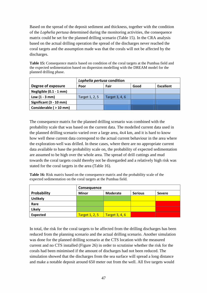
47

Based on the spread of the deposit sediment and thickness, together with the condition

of the Lophelia pertusa determined during the monitoring activities, the consequence

matrix could be set for the planned drilling scenario (Table 15). In the CRA analysis

based on the actual drilling operation the spread of the discharges never reached the

coral targets and the assumption made was that the corals will not be affected by the

discharges.

Table 15: Consequence matrix based on condition of the coral targets at the Pumbaa field and

the expected sedimentation based on dispersion modelling with the DREAM model for the

planned drilling phase.

Degree of exposure

Lophelia pertusa condition

Poor Fair Good Excellent

Negligible (0.1 - 1 mm)

Low (1 - 3 mm) Target 1, 2, 5 Target 3, 4, 6

Significant (3 - 10 mm)

Considerable ( > 10 mm)

The consequence matrix for the planned drilling scenario was combined with the

probability scale that was based on the current data. The modelled current data used in

the planned drilling scenario varied over a large area, 4x4 km, and it is hard to know

how well these current data correspond to the actual current behaviour in the area where

the exploration-well was drilled. In these cases, where there are no appropriate current

data available to base the probability scale on, the probability of expected sedimentation

are assumed to be high over the whole area. The spread of drill cuttings and mud

towards the coral targets could thereby not be disregarded and a relatively high risk was

stated for the coral targets in the area (Table 16).

Table 16: Risk matrix based on the consequence matrix and the probability scale of the

expected sedimentation on the coral targets at the Pumbaa field.

Probability

Consequence

Minor Moderate Serious Severe

Unlikely Rare Likely Expected Target 1, 2, 5 Target 3, 4, 6

In total, the risk for the coral targets to be affected from the drilling discharges has been

reduced from the planning scenario and the actual drilling scenario. Another simulation

was done for the planned drilling scenario at the CTS location with the measured

current and no CTS installed (Figure 26) in order to scrutinise whether the risk for the

corals had been minimised if the amount of discharges had not been reduced. The

simulation showed that the discharges from the sea surface will spread a long distance

and make a notable deposit around 650 meter out from the well. All five targets would

48

thereby have been affected, if the current would have had the direction towards the

corals.

Figure 26: Output from the DREAM model for the planned drilling scenario modelled with

measured current data from the monitoring program during the actual drilling operation.

Parameters; grid size 4x4 m, time step = 5 minute, measured current and default values in the

near field model.

49

5 DISCUSSION In this study two different dispersion models were used in order to determine how well

they managed to simulate the actual spread of drilling discharges at the Pumbaa field on

the NSC. Comparison with monitoring data was done in an attempt to validate the

simulations. Two scenarios have been studied, the planned drilling scenario and the

actual drilling scenario, in order to evaluate whether decisions in the drill planning

process reduced the risk for the coral targets to be affected by the drilling discharges

released during the actual drilling operation.

5.1 THE DISPERSION MODELS AND COMPARISON WITH MONITORING DATA

The actual drilling scenario modelled with the MUDFATE model and the DREAM

model with the CTS installed, had the best match judging by the correlation between the

simulations and the 200 mg/kg barium level (Figure 22 and Figure 23). The actual

drilling scenario for the DREAM model with the CTS installed also had the best fit

comparing the spread of sediment deposit with the sediment samples of highest barium

concentration. However, this simulation should match the actual spread of drilling

discharges best, considering the fact that the CTS was used and that measured current

data were obtained from the actual drilling campaign. A good correlation between the

current directions in the measured current data and the directions of spread of drilling

discharge deposit for each drill section released could be seen (compare Figure 12 and

Figure 20).

In the simulations for the planned drilling scenarios the spread of drilling discharges

deposit was limited to a narrow area and a large amount of the sediment deposited was

outside the grid (Figure 15, Figure 16 and Figure 17), and thereby also outside the 200

mg/kg barium level, which makes the match with the monitoring results inaccurate. The

amount of drill cuttings released in the planned drilling scenario was higher than for the

actual drilling scenario. Moreover, the current data used in the different planned drilling

scenarios, the modelled current and the interpolated current data, corresponded to an

area of 4x4 km which differed from the measured current data, which were obtained

during the actual drilling operation from the actual drilling area, at a height of 2 and 10

m above the sea floor. Hence, a lower correlation should be expected between the

monitoring data and simulated data regarding the planned drilling scenario.

Considering the distance of the spread of the sediment deposit according to the

guidelines made by Ulfsnes et al. (2012a), as estimated from experience and simulation

modelling by the DREAM model, the suggested distance for deposition of sediment of

0.1 -1 mm is within the range of 250 – 1,000 m. The distances in all simulations for the

planned drilling scenario are probably wider than 1,000 m (Table 11). The re-simulated

planned drilling scenario with the modelled current in the CRA analysis showed a

spread with a distance over 1,200 m (Figure 24). The simulation done for the actual

drilling scenario in the MUDFATE model showed a spread around 130 m, which

regarding to the guidelines is too short (Table 11). Also, a low sediment deposit

thickness was obtained in the same simulation. A peak of deposited sediment could be

seen along the current around 30 m from the discharge location, which is further away

50

from the discharge location than for the other simulations where the pile was modelled

some few meters from the outlet (Table 13). The reason for the underestimated distance

from the outlet to the pile is a problem in the code that requires the model to generate all

clouds with a centroid above the seabed. The height for the clouds had to be adjusted,

which caused the small distance to where the pile was building up. Computational

Hydraulics and Transport (CHT) has tried to eliminate this error, and in recent

simulations higher mounds at the discharge location have been obtained with a sediment

thickness around 250 mm, and a peak of 521 mm (Teeter, 2013, Pers. Comm.).

Compared to the other simulations made in the DREAM model these are still low

values. The fact that the simulation was run without the near field model may also have

contributed to the low modelled sediment thickness.

In an attempt to quantify the accuracy of the simulation for the actual drilling scenario,

the deposition of barium was calculated and compared to the barium concentration

obtained for the 20 sediment samples taken during the monitoring program. The barium

content obtained for the actual drilling scenario using the MUDFATE model was 4.2

g/m2, and using the DREAM model with the CTS installed the barium content was 38.2

g/m2. Rye et al. (2012) calculated the barium content for the measured sediment

samples to 6.13 g/m2, and the barium content for their simulation with the DREAM

model was 92.84 g/m2. It should be noted that the DREAM model still overestimated

the output, which is probably due to the announced “crater effect” by Rey et al. (2012).

However, in this study the barium content seemed to be overestimated by a factor of six

instead of 15. In the analysis of the sediment thickness and pile height, the simulations

done with the DREAM model for the actual case with the CTS had a higher average

deposition inside an area of 20 m than the simulations without the CTS, indicating that

the crater effect was higher in a case with a CTS installed (Table 13). This could also

have been obtained in the barium content calculations, where the barium content for the

scenario without the CTS was 22.0 g/m2. The overestimation for the scenario without

the CTS installed was by a factor around four.

The reason for the different results for the DREAM model simulations in this study and

runs done by Rye et al. (2012), is either different calculation methods to get the barium

content or the setup of parameters in the DREAM model. The simulation made by Rye

et al. (2012) was modelled using a grid of 1x1 m, generated for a larger amount of

particles and during a longer time (Rye, 2013, Pers. Comm.), which can have a

significant effect on the output. Particle tracking models are in general also

probabilistic, which means that even for the same setup of parameters the same

simulation can give differences in output. The barium content obtained using the

MUDFATE model was very close to the measured barium content. Important to

mention is also that the barium content for the MUDFATE model was obtained from

the deposit of the two finest grain classes which means that the actual spread of barite is

probably higher and therefore also the barium concentration. In addition, the fact that

the deposit in general was low and due to the code problem, the value most likely

51

should be higher and will thereby probably will overestimate the actual spread of

drilling discharges.

In total, this study has failed to determine which one of the models makes the best

simulations of drilling discharge. More time must be spent on each model in order to get

more comparable simulations. However, when using a CTS during a discharge situation

a crater will build up quite rapidly and most likely minimise the spread of cuttings and

mud, which is confirmed by the visual survey done during the actual drilling operation.

The simulations indicated this by overestimating the barium content observed in the

DREAM model simulations. Whether the MUDFATE model is overestimating the

barium content is difficult to determine regarding the underestimation of the distance to

the pile and possible sediment deposit.

When making risk assessment it is, however, good to have an overestimation of the

sediment deposit rather than values lower than the actual spread. It is difficult to predict

before the actual event how the actual situation for the drilling operation will be at that

specific time and place, independently on how good the input data are. The most

important subsequent step is then to validate the modelled simulations based on

experience from both earlier simulated projects and monitoring surveys, before model

simulations are used in the CRA analysis.

Pivel et al. (2008, p. 20) have made a similar research where they compared modelled

results, simulated with the OOC Model (Offshore Operators Committee Mud and

Produced Water Discharge Model), with monitoring data on a drilled well outside

Brazil. They conclude that the accuracy of the input data has a large effect on the

prediction ability of the model and that even small uncertainties in the discharge

activities can have a large effect on the prediction of the dispersion of drilling

discharges. Pivel et al. (2008, p. 20) also concludes that it is important to validate the

results and to do several simulations depending on the accuracy of the input data and

how good the knowledge of the hydrodynamics is in the sit specific area.

5.2 THE CRA ANALYSIS

In the CRA analysis a relatively high risk could be determined for the coral targets in

the area of the Pumbaa field for the planned drilling scenario (Figure 24). A sediment

deposit thickness between 1 – 3 mm could be expected on the coral targets, meaning a

minor or moderate effect depending on the condition of the corals. However, if the

discharge location still had been on the drilling location, the corals would have been in a

higher sediment category. This means that the risk for the corals has been reduced by

moving the discharge location 300 m north-west from the actual drilling location, where

no other corals have been monitored.

For the actual drilling scenario, no risk could be determined for the coral targets in the

CRA analysis (Figure 25). This means that the risk for the corals has been reduced from

the planned drilling scenario to the actual drilling scenario. The decision to reduce the

number of drilled sections and thereby reducing the amount of cuttings released, 703

tonnes of cuttings in the planning phase compared to 139 tonnes in the actual drilling

52

scenario, reduced the risk for the corals to be affected by the drilling discharges. The

corals would still not have been affected from the drilling discharges in the actual

drilling scenario if the drilling discharges would have been released at the drilling

location. The closest coral target is located about 300 m from the drilling location and

the dimension of the sediment category of 0.1 - 1 mm, is about 260 m around the

discharge location. However, the mass balance indicates that a lot of discharges were

drifting further away from the discharge location. This sediment deposit would probably

be lower than 0.1 mm and not affecting the corals significantly, but it is still uncertain

whether the sediment and added substances can have undesirable long-term effects on

the corals and the environment.

The re-simulation of the planned drilling scenario at the CTS location modelled with the

measured current data and no CTS installed (Figure 26), confirms that the decision of

reducing the amount of cuttings was a beneficial decision. The simulation shows a

deposit from the discharge from the sea surface (18 m depth), which will spread a long

distance and make a notable deposit around 650 m out from the well. If the current

would have had the direction towards the corals in this case, all five targets would have

been affected by a sediment deposit over 0.1 mm.

When comparing the simulations for the planned drilling scenario to the actual drilling

scenario, the amount of discharge and the current data seemed to affect the modelled

output the most, and also the output of the CRA analysis. Due to the fact that the current

data are used in the CRA analysis, both in the dispersion simulations and as a basis for

the probability scale, it is very important that the current data are good and

representative for the discharge location. The way the current data are used as a basis

for the probability scale should also be scrutinised in further studies. This is however

not within the scope of this study.

5.3 DISPERSION MODELLING - CHOICE OF INPUT PARAMETERS

To perform good dispersion modelling, as any modelling, a fundamental prerequisite is

to have good input data. However, even if the input data are good, the setup of

parameters in the model needs to be calibrated in an appropriate way to make the output

correct. This step is not always easy and the more detailed data put into the model, the

more important will the setup of parameters be. During the simulations with the

DREAM model, a distinguishable difference in the output has been seen when choosing

different time steps (APPENDIX III – Simulations with Changed Time Step and Grid

Size in the DREAM Model).

For a long time step (5 minutes or 1 minutes) the discharges seemed to spread more in

the directions of the CTS and for a short time step (10 seconds or 5 seconds), the

discharge seemed to increasingly follow the directions of the current. One theory is that

when using a long time step the particles manage to travel over several grid squares

before being counted by the model. The reason in this case is most likely due to the

initial velocity from the CTS forcing the particles to travel the long distance, when

choosing a long time step. When using a shorter time step the particles do not manage to

53

travel more than one grid box before they are counted, and the spread is then to a greater

extent affected by the directions of the current, which affects the behaviour of the

particle in every time step.

Regarding how the models handle the discharge in the water column, the major

difference is in how the two models simulate and follow the particles in the water

column. The DREAM model follows every discharge particle with different setups of

properties. In contrast, the MUDFATE model, instead of following particles, follows a

cloud of particles. These clouds are three-dimensional and are assumed to have

Gaussian distribution of particle concentration where each cloud has a distinct particle

settling. In the MUDFATE model, there are two time step functions for the clouds; one

for the frequency of launching the clouds (Input from a near field model) and the second

for dispersion which governs the frequency at which the clouds are advected, diffused

and settled. The same time steps are more or less available in the DREAM model,

where one time step can be set in the near field module and one in far field model,

where the ambient conditions in the water column are affecting the particle.

The discharge from the CTS had a velocity of 2 m/s according to Rye et al. (2012) and a

distinguishable jet-plume trajectory could be noted in tens of meters from the CTS.

During the simulation made using the DMUFATE model for the actual drilling scenario

an initial velocity of 1.0 m/sec with a plume that touched the bed with a velocity of 0.22

m/s could be distinguished after about 1.8 m travel distance. The situation in

DMUFATE indicated a risk for the suspension to be moved and mixed by the ambient

current rather than by its own initial momentum and density effects, and the decision

was made not to use the near field model in the further simulations (Teeter, 2013, Pers.

Comm.). The fact that a pile was building up close to the discharge location was,

however, the main reason for not using the DMUFATE model to predict the near field

behaviour of the discharge according to Teeter (2013, Pers. Comm.). The use of the near

field module in the DREAM model could therefore be the main reason for the

overestimation.

The result obtained by Rye et al (2012) is also very different from the simulations made

with the DREAM model in this study where no distinct spread of the deposit could be

seen in the CTS directions (Figure 20). However, in the simulations done with a longer

time step (5 minute and 1 minute) a jet-trajectory has been observed (APPENDIX III –

Simulations with Changed Time Step and Grid Size in the DREAM Model). A velocity

of 2 m/s will transport even the larger particles for a shorter distance before they are

allowed to settle down on the sea floor. With a grid of 4x4m, the velocity gives a travel

time of two seconds over one grid square. Regarding the simulations with the high time

step, the CTS velocity most likely contributed to the spread in CTS directions.

However, setting the time step too low can also contribute to rounding errors in the

model (Rye, 2013, Pers. Comm.). The possibility to set a time step in the near field

module makes is possible to not have to set the time step in the far field model to short.

The near field model handles the behaviour of the spread closest to the discharge

location and thereby the initial velocity from the CTS. However, the fact of rounding

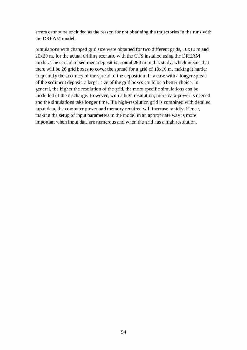
54

errors cannot be excluded as the reason for not obtaining the trajectories in the runs with

the DREAM model.

Simulations with changed grid size were obtained for two different grids, 10x10 m and

20x20 m, for the actual drilling scenario with the CTS installed using the DREAM

model. The spread of sediment deposit is around 260 m in this study, which means that

there will be 26 grid boxes to cover the spread for a grid of 10x10 m, making it harder

to quantify the accuracy of the spread of the deposition. In a case with a longer spread

of the sediment deposit, a larger size of the grid boxes could be a better choice. In

general, the higher the resolution of the grid, the more specific simulations can be

modelled of the discharge. However, with a high resolution, more data-power is needed

and the simulations take longer time. If a high-resolution grid is combined with detailed

input data, the computer power and memory required will increase rapidly. Hence,

making the setup of input parameters in the model in an appropriate way is more

important when input data are numerous and when the grid has a high resolution.

55

6 CONCLUSIONS The simulation of the actual drilling scenario for the DREAM model with the CTS

installed had the best fit judged by the correspondence between the simulation and the

200 mg/kg barium level (Figure 22), and when comparing the spread of sediment

deposit with the empirical sediment samples of highest barium concentration. High

correlation could also be noted between the current directions in the measured current

data and the directions of spread of drilling discharges for each drill section released.

The simulations done for the planned drilling scenario showed less correspondence with

the monitoring data than simulations for the actual drilling scenario.

To perform good dispersion modelling it is important that the input data are

representative for the actual drilling operation area. Hence, accurate input data are

important for the CRA analysis in order to get good estimates of the risk-situation for

the corals. However, when modelling the dispersion of drilling discharges, the setup of

input parameters in the dispersion models is most important. The conclusion is that

when modelling the dispersion of drilling discharges for a CRA analysis it is important

that the simulation results are validated both for the setup of parameters in the

dispersion models and that results conform to experiences from earlier simulated

projects and monitoring surveys. Determining which one of the models, the DREAM

model or the MUDFATE model, simulates the dispersion of drilling discharges best

could not be done based on the simulations made in this study.

The amount of discharge and the current data seemed to have largest effect on the

modelled output of sediment deposit from drilling discharges. Together with the

location of the discharge point and the condition of the coral targets, these were the

factors that had the most important impact on the result from the CRA analysis. It has

also been seen in this study that when discharges were released through a CTS a crater

built up quite rapidly close to the CTS, thus reducing the spread of cuttings and mud.

The dispersion models do not account for this pile and thereby overestimate the deposit

of sediment in the area. This is the fact the case for the DREAM model. The extent to

which similar overestimates appear for the MUDFATE model has, however, not been

investigated further.

In the CRA analysis, a relatively high risk could be assessed for the coral targets in the

area of the Pumbaa field for the planned drilling scenario (Figure 24), although for the

actual drilling scenario no risk could be determined (Figure 25). This means that by

moving the discharge location 300 m north-east from the actual drilling location and by

reducing the amount of drilling discharges, the risk for the corals to be affected from the

drilling operation was reduced. These results also show that the environmental actions

in the drill planning process were necessary to reduce the risk for the coral targets.

56

REFERENCES Aaserød, M. I., Bjørgesæter, A., Eggen, B. & Midtsund, G., 2009. Environmental Risk

Assessment and Oil Spill Emergancy Preparedness Analyses of well 6407/12-2 Pumbaa,

Stavanger: GDF SUEZ E&P Norge AS.

CHT, 2012a. User's Guid for Far Field Fate of Drilling Mud (MUDFATE), Mississippi:

Computional Hydraulics and Transport (CHT).

CHT, 2012b. User's Guide and Documentetion for the DMPLM and MUDFATE Near-

field Drilling Mud Dispersion Models, Mississippi: Computational Hydraulics and

Transport (CHT).

DNV, 2013. Drilling in sensitive areas - A guideline for "best practices" keeping focus

on the seabed environment, Høvik: Det Norske Veritas - Environmental Risk

Management.

Furgo Survey AS, 2008. Rig Site Survey NOCS Block 6407/12-2 Pumbaa Survey

Periode: 19 August - 23 August 2008 Report Number: 9749V1.1 Voume 1: Habitat

Investigation, Stavanger: Gaz de France Norge AS.

ISO, 2009. ISO 31000 Risk managment - Principle and guidlines, Switzerland:

International Standard Organization (ISO).

KLif, 2009. TA2586 Guidelines for environmentel monitoring of the petroleum

activities on the Norwegian continental shelf, Oslo: The Climate and Pollution Agency

(KLif).

Kålås, J. A., Viken, Å., Henriksen, S. & Skjelseth, S., 2010. The 2010 Norwegian Red

List of specis. Trondheim: Norwegian Biodiversity Information Centre.

Larsson, A. I. & Purser, A., 2011. Sedimentation on the cold-water coral Lophelia

pertusa: Cleaning efficiency from natural sediment and drill cuttings. Marine Pollution

Bulletin, Volume 62, pp. 1159 – 1168.

MAREANO, 2013. MAREANO - Collecting Marine Knowledge.

http://www.mareano.no/en/start (2013 03 19)

MPE & NPD, 2012. Fakta 2012 Norsk petroleumsvirksomhet. Oslo: Ministry of

Petroleum and Energy (MPE) & Norwegian Petroleum Directorate (NPD).

Ministry of Petroleum and Energy, 2013a. LOV 1996-11-29 nr 72: Lov om

petroleumsvirksomhet [petroleumsloven].

http://www.lovdata.no/all/hl-19961129-072.html (2013 03 08).

Ministry of Petroleum and Energy, 2013b. FOR 1997-06-27 nr 653: Forskrift til lov om

petroleumsvirksomhet.

http://www.lovdata.no/cgi-wift/ldles?doc=/sf/sf/sf-19970627-0653.html (2013 03 08).

57

MPE, 1981. Ministry of the Environment, Act of 13 March 1981 No.6 Concerning

Protection Against Pollution and Concerning Waste.

http://www.lovdata.no/all/hl-19810313-006.html#49 (2013 04 04).

Nellemann, C., Hain, S. & Adler, J., 2008. In Dead Water – Merging of climate change

with pollution,, Norway: United Nations Environment Programme, GRID-Arendal.

NPD, 2008. Production licence – licence to explore, discover and produce.

http://www.npd.no/en/Topics/Production-licences/Theme-articles/Production-licence--

licence-to-explore-discover-and-produce-/ (2013 03 08).

Øfjord, G. D., Lind, M. J. & Skaare, B. B., 2012. Håndtering av borekaks i områder

med sårbar bunnfauna, Oslo: The Climate and Pollution Agency (Klif).

OSPAR Agreement, 2012-06. The OSPAR List of Substances/Preparations Used and

Discharged Offshore which are Considered to Pose Little or No Risk to the

Environment (PLONOR), s.l.: OSPAR Commision.

OSPAR Commission, 2013a. Introduction.

http://www.ospar.org/content/content.asp?menu=00310108000000_000000_000000

(2013 04 05).

OSPAR Commission, 2013b. Offshore Chemicals.

http://www.ospar.org/content/content.asp?menu=00850305350000_000000_000000

(2013 04 04).

OSPAR, 2008. OSPAR List of Threatened and/or Declining Species and Habitats

(Reference Number: 2008-6, Replaces agreement 2004-6), s.l.: The Convention for the

Protection of the marine Environment of the North-East Atlantic.

OSPAR, 2010. OSPAR Recommendation 2010/9 on furthering the protection and

restoration of coral gardens in the OSPAR Maritime Area, s.l.: OSPAR Commission.

Pivel, M. A. G., Freitas, C. M. D. S., Comba, J. L. D., 2008. Modeling the discharge of

cuttings and drilling fluids in a deep-water environment, Deep Sea Research Part II:

Topical Stuides in Oceanography, Volume 56, pp. 12 – 21.

PSA, 2013. Petroleum Safety Authority Norway.

http://www.ptil.no/activities/category399.html?lang=en_US#_Toc345662833 (2013 04

04).

Research Council of Norway, 2012. Long-term effects of discharges to sea, Oslo:

Research Council of Norway.

Roberts, J. M., Andrew, W., André, F. & Stephen, C., 2009. Cold-Water Corals – The

Biology and Geology of Deep-Sea Habitats. New York: Cambridge University Press.

58

Rye, H. & Ditlevsen, M. K., 2009. EIF and deposition calculations for exploration

drilling at the Pumbaa Exploration Field (PL469) Final report, Trondheim: SINTEF

Materials and Chemistry.

Rye, H., Ditlevsen, M. K., Moe, J. A. & Løkken, M., 2012. SPE 1566775: Simulation

Of Concentration and Depositions of Particle Matter Caused by Drilling Discharges.

Comparison Between Field Measurements and Simulation Results at Coral Locations,

s.l.: SPEA/APPEA International.

Rye, H., Reed, M., Durgut, I. & Ditlevsen, M. K., 2006. ERMS Report No.18

Documention report for the revised DREAM model, Trondheim: SINTEF Materials and

Chemistry.

Schlumberger, 2013. Oilfield Glossary.

http://glossary.oilfield.slb.com/en/Terms/k/kick.aspx (2013 05 06).

Sheppard, C. R. C., Davy, S. K. & Graham, M. P., 2009. The Biology of Coral Reefs.

New York: Oxford University Press.

Standard Norge, 2009. NS 9435:2009 Water quality - Visual seabed survey using

remotely operated and towed observation gear fro collection of environmental data, s.l.:

Standard Norge.

Ulfsnes, A., Hugland, J. K. & Weltzien, R., 2012a. Monitoring of Drilling Activities in

Areas with Presence of Cold Water Corals., Oslo: Det Norske Veritas AS.

Ulfsnes, A., Møskeland, T. & Øivin, A., 2012b. SPE-156543: Coral Risk Assessment -

Tool Development, s.l.: SPE International/APPEA.

Ulfsnes, A., Sverdrup, L. & Fjukmoen, Ø., 2010. Monitoring of drilling at Pumbaa,

Oslo: Det Norske Veritas AS.

Vanoni, V. A., 2006. ASCE Manuals and reports on Engineering Practice No. 54

Sedimentation Engineering. 2 red. Virginia: American Society of Civil Engineers.

Oral references

Lyngrot, Steinar, 2013. Consultant, Det Norske Veritas. Course - 2666 “Petroleum

Technology & Geoscience” (15 – 16 April 2013).

Rye, Henrik, 2013. Consultant, SINTEF.

Teeter, Allen, 2013. Consultant, Computational Hydraulics and Transport (CHT).

59

APPENDIX I - Input Data for the Planned Drilling Scenario Input data for exploration drilling in the planning phase at the Pumbaa location (PL 469) in the Norwegian Sea (Table I-1 to Table I-4). The data

is taken from the report “EIF and deposition calculations for exploration drilling at the Pumbaa Exploration Field (PL469)”made by SINTEF

(Rye & Ditlevsen, 2009).

Table I-1: Input data for the planned base case for the exploration drilling.

Drilling section 42" 36" 9,875" pilot 26" 17,5" 12,25"

Start of discharge1 (h) 0 24 24 24 24 24

Section length (m) 22 50 478 386 190 571

Drilling rate (m/h) 10 10 25 20 25 25

Discharge depth 1 m

above sea floor 1 m

above sea floor 1 m

above sea floor 1 m

above sea floor 18 m

below sea surface 18 m

below sea surface

Diameter of outlet opening (m) 1.0668 0.9144 0.254 0.66 0.4 0.4

Orientation of outlet opening Vertically upwards

Vertically upwards

Vertically upwards

Vertically downwards

Vertically downwards

Vertically downwards

Duration2 2.2 hours 5 hours 19.12 hours 19.3 hours 7.6 hours 22.84 hours

Components Compounds Amounts (tonnes)

Amounts (tonnes)

Amounts (tonnes)

Amounts (tonnes)

Amounts (tonnes)

Amounts (tonnes)

Particles Cuttings 49.16 82.086 58.6594 330.545 73.71 108.439

Mud Particles Bentonite 6.43 10.82 16.38 47.81 0 0

Mud Particles Barite 31.62 53.29 28.58 123.88 36.76 143.27

Sum MUD3: 78.05 137.13 293.96 762.69 147.67 269.4

1) Start of discharge - Time elapsed before starting discharge for this section/ time passed after the previous discharge ends. The start date is 01.11.2004.

2) Duration - Automatically calculated by the DREAM model

3) Sum MUD - Includes water and PLONOR chemicals in addition. Cuttings particles are not and should not be included in this parameter.

60

Table I-2: Input data over grain size distribution of cuttings particles. The values are from Saga

(1994) measured during an exploration drilling in the Barents Sea (Rye & Ditlevsen, 2009). In

the MUDFATE model these fractions are merged into five fractions.

Table I-3: Input data over grain size distribution of Barite particles. The values are from Saga

(1994) measured from the shaker up on the rig during an exploration drilling in the Barents Sea

(Rye & Ditlevsen, 2009). In the MUDFATE model these fractions are merged into five

fractions.

Diameter (µm) Weight (%) Accumulated weight

0 - 100 % Density (g/cm3)

1 < > 2 30 30 4.2

2 < > 3 10 40 4.2

3 < > 5 10 50 4.2

5 < > 9 10 60 4.2

9 < > 14 10 70 4.2

14 < > 18 10 80 4.2

18 < > 28 10 90 4.2

28 < > 50 10 100 4.2

Diameter (µm) Weight (%) Accumulated weight

0 - 100 % Density (g/cm3)

7 10 10 2.5

15 10 20 2.5

25 10 30 2.5

35 10 40 2.5

50 10 50 2.5

75 10 60 2.5

200 10 70 2.5

600 10 80 2.5

3000 10 90 2.5

7000 10 100 2.5

61

Table I-4: Input data over grain size distribution of Bentonite particles. The values are

compared with the grain size distribution for Barite from Saga (1994) and assumed to be similar

(Rye & Ditlevsen, 2009). In the MUDFATE model these fractions are merged into five

fractions.

Diameter (µm) Weight (%) Accumulated weight

0 - 100 % Density (g/cm3)

1 < > 2 30 30 2.5

2 < > 3 10 40 2.5

3 < > 5 10 50 2.5

5 < > 9 10 60 2.5

9 < > 14 10 70 2.5

14 < > 18 10 80 2.5

18 < > 28 10 90 2.5

28 < > 50 10 100 2.5

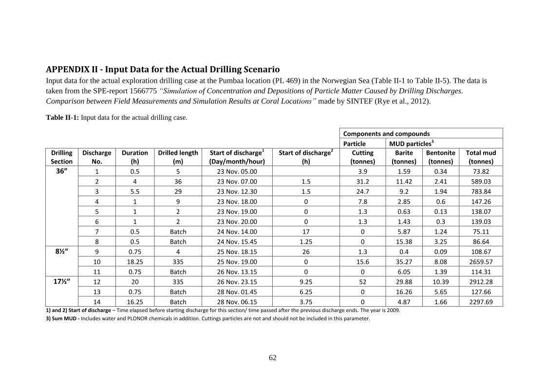
62

APPENDIX II - Input Data for the Actual Drilling Scenario Input data for the actual exploration drilling case at the Pumbaa location (PL 469) in the Norwegian Sea (Table II-1 to Table II-5). The data is

taken from the SPE-report 1566775 “Simulation of Concentration and Depositions of Particle Matter Caused by Drilling Discharges.

Comparison between Field Measurements and Simulation Results at Coral Locations” made by SINTEF (Rye et al., 2012).

Table II-1: Input data for the actual drilling case.

Components and compounds

Particle MUD particles3

Drilling Section

Discharge No.

Duration (h)

Drilled length (m)

Start of discharge1 (Day/month/hour)

Start of discharge2 (h)

Cutting (tonnes)

Barite (tonnes)

Bentonite (tonnes)

Total mud (tonnes)

36” 1 0.5 5 23 Nov. 05.00

3.9 1.59 0.34 73.82

2 4 36 23 Nov. 07.00 1.5 31.2 11.42 2.41 589.03

3 5.5 29 23 Nov. 12.30 1.5 24.7 9.2 1.94 783.84

4 1 9 23 Nov. 18.00 0 7.8 2.85 0.6 147.26

5 1 2 23 Nov. 19.00 0 1.3 0.63 0.13 138.07

6 1 2 23 Nov. 20.00 0 1.3 1.43 0.3 139.03

7 0.5 Batch 24 Nov. 14.00 17 0 5.87 1.24 75.11

8 0.5 Batch 24 Nov. 15.45 1.25 0 15.38 3.25 86.64

8½“ 9 0.75 4 25 Nov. 18.15 26 1.3 0.4 0.09 108.67

10 18.25 335 25 Nov. 19.00 0 15.6 35.27 8.08 2659.57

11 0.75 Batch 26 Nov. 13.15 0 0 6.05 1.39 114.31

17½“ 12 20 335 26 Nov. 23.15 9.25 52 29.88 10.39 2912.28

13 0.75 Batch 28 Nov. 01.45 6.25 0 16.26 5.65 127.66

14 16.25 Batch 28 Nov. 06.15 3.75 0 4.87 1.66 2297.69 1) and 2) Start of discharge – Time elapsed before starting discharge for this section/ time passed after the previous discharge ends. The year is 2009.

3) Sum MUD - Includes water and PLONOR chemicals in addition. Cuttings particles are not and should not be included in this parameter.

63

Table II-2: Input data over grain size distribution of cuttings for 36" drilling section and 8½"

pilot hole. Data is based on analysis of the actual cuttings from the drilling activities at Pumbaa

carried out by Optipro (Rye et al., 2012). In the MUDFATE model these fractions are merged

into five fractions.

Diameter (µm) Weight (%) Accumulated weight

(0 - 100 %) Density (g/cm3)

(1 - 25) 2,2 2,2 3

25 - 32 7,99 10,19 3

32 - 63 7,05 17,24 3

63 - 80 8,63 25,87 3

80 - 100 32,58 58,45 3

100 - 200 14,43 72,88 3

200 - 315 10,45 83,33 3

315 - 425 4,7 88,03 3

425 - 500 5,66 93,69 3

500 - 630 3,35 97,04 3

630 - 2000 2,96 100 3

Table II-3: Input data over grain size distribution of cuttings for 17½" drilling section. Data is

based on analysis of the actual cuttings from the drilling activities at Pumbaa carried out by

Optipro (Rye et al., 2012). In the MUDFATE model these fractions are merged into five

fractions.

Diameter (µm) Weight (%) Accumulated weight

0 - 100 % Density (g/cm3)

45 - 75 7,23 7,23 3

75 - 90 14,94 22,17 3

90 - 125 24,69 46,86 3

125 - 250 7,58 54,44 3

250 - 500 1,96 56,4 3

500 - 1000 7,24 63,64 3

1000 - 2000 13,03 76,67 3

2000 - 4000 4,35 81,02 3

4000 - 8000 18,98 100 3

64

Table II-4: Input data over grain size distribution of Barite particles. The values are from Saga

(1994) measured from the shaker up on the rig during an exploration drilling in the Barents Sea

(Rye et al., 2012). In the MUDFATE model these fractions are merged into five fractions.

Diameter (µm) Weight (%) Accumulated weight

0 - 100 % Density (g/cm3)

1 < > 2 25 25 4.2

2 < > 7 25 50 4.2

7 < > 10 25 75 4.2

10 < > 25 5 80 4.2

25 < > 30 5 85 4.2

30 < > 33 5 90 4.2

33 < > 40 4 94 4.2

40 < > 45 3 97 4.2

45 < > 55 2 99 4.2

55 < > 65 1 100 4.2

Table II-5: Input data over grain size distribution of Bentonite particles. The values are

compared with the grain size distribution for Barite from Saga (1994) and assumed to be similar

(Rye et al., 2012). In the MUDFATE model these fractions are merged into five fractions.

Diameter (µm) Weight (%) Accumulated weight

0 - 100 % Density (g/cm3)

1 < > 2 25 25 2.5

2 < > 7 25 50 2.5

7 < > 10 25 75 2.5

10 < > 25 5 80 2.5

25 < > 30 5 85 2.5

30 < > 33 5 90 2.5

33 < > 40 4 94 2.5

40 < > 45 3 97 2.5

45 < > 55 2 99 2.5

55 < > 65 1 100 2.5

65

APPENDIX III – Simulations with Changed Time Step and Grid Size

in the DREAM Model In the DREAM model the actual drilling scenario with the CTS installed has been

simulated for different setup of parameters to analyse how sensitive the model is for

changes in parameters. Seven simulations have been made for different setup of time

step and grid size (Table III-1; Figure III-1 to Figure III-7). Time step in the near field

module have been change from default value (5 s) in some simulations.

Table III-1: The different simulations made with the DREAM model for the actual drilling

scenario. Parameters such as size of grid, time step and near field model parameters have been

varied in the simulations.

Size of Grid Time Step Current Near Field Module Comments

4x4 m 5 s Measured Default

4x4 m 10 s Measured Change Used in CRA

4x4 m 20 s Measured Default

4x4 m 1 minute Measured Default

4x4 m 5 minute Measured Default

10x10 m 10 s Measured Changed

20x20 m 10 s Measured Changed

Figure III-1: Model output from simulation with the DREAM model for the actual drilling

scenario with the CTS installed. Parameters; grid size 4x4 m, time step = 5 s, measured current

and default values in the near field model.

66

Figure III-2: Model output from simulation with the DREAM model for the actual drilling

scenario with the CTS installed. Parameters; grid size 4x4 m, time step = 10 s, measured current

and time step changed to 0.1 s in the near field model.

Figure III-3: Model output from simulation with the DREAM model for the actual drilling

scenario with the CTS installed. Parameters; grid size 4x4 m, time step = 20 s, measured current

and default values in the near field model.

67

Figure III-4: Model output from simulation with the DREAM model for the actual drilling

scenario with the CTS installed. Parameters; grid size 4x4 m, time step = 1 minute, measured

current and default values in the near field model.

Figure III-5: Model output from simulation with the DREAM model for the actual drilling

scenario with the CTS installed. Parameters; grid size 4x4 m, time step = 5 minute, measured

current and default values in the near field model.

68

Figure III-6: Model output from simulation with the DREAM model for the actual drilling

scenario with the CTS installed. Parameters; grid size 10x10 m, time step = 10 s, measured

current and time step changed to 0.1 s in the near field model.

Figure III-7: Model output from simulation with the DREAM model for the actual drilling

scenario with the CTS installed. Parameters; grid size 20x20 m, time step = 10 s, measured

current and time step changed to 0.1 s in the near field model.