dispersion of a tracer in the deep gulf of mexico

RESEARCH ARTICLE10.1002/2015JC011405

Dispersion of a tracer in the deep Gulf of Mexico

James R. Ledwell1, Ruoying He2, Zuo Xue3, Steven F. DiMarco4, Laura J. Spencer4, and Piers Chapman4

1Woods Hole Oceanographic Institution, Woods Hole, Massachusetts, USA, 2Department of Marine, Earth, andAtmospheric Sciences, North Carolina State University, Raleigh, North Carolina, USA, 3College of the Coast andEnvironment, Louisiana State University, Baton Rouge, Louisiana, USA, 4Department of Oceanography, Texas A&MUniversity, College Station, Texas, USA

Abstract A 25 km streak of CF3SF5 was released on an isopycnal surface approximately 1100 m deep,and 150 m above the bottom, along the continental slope of the northern Gulf of Mexico, to study stirringand mixing of a passive tracer. The location and depth of the release were near those of the deep hydrocar-bon plume resulting from the 2010 Deepwater Horizon oil well rupture. The tracer was sampled between 5and 12 days after release, and again 4 and 12 months after release. The tracer moved along the slope at firstbut gradually moved into the interior of the Gulf. Diapycnal spreading of the patch during the first 4 monthswas much faster than it was between 4 and 12 months, indicating that mixing was greatly enhanced overthe slope. The rate of lateral homogenization of the tracer was much greater than observed in similarexperiments in the open ocean, again possibly enhanced near the slope. Maximum concentrations found inthe surveys had fallen by factors of 104, 107, and 108, at 1 week, 4 months, and 12 months, respectively,compared with those estimated for the initial tracer streak. A regional ocean model was used to simulatethe tracer field and help interpret its dispersion and temporal evolution. Model-data comparisons show thatthe model simulation was able to replicate statistics of the observed tracer distribution that would beimportant in assessing the impact of oil releases in the middepth Gulf.

1. Introduction

The Gulf of Mexico has been the subject of intensified study since the massive release of oil from the rup-tured Deepwater Horizon well in 2010 (see Lubchenco et al. [2012] for an overview). As a part of thatresearch effort, we have carried out a tracer release experiment starting along the northern slope of theGulf not far from the rupture and at a depth of approximately 1100 m, similar to the depth of the deepplume from the rupture, as observed by Camilli et al. [2010]. The goals of the tracer experiment are to studythe processes of dispersion in the middepth Gulf and to contribute to the improvement of numerical fore-cast models of circulation and dispersion. A practical motivation for this research is to provide better infor-mation to those interested in commercial development of Gulf resources, to regulators, and to thoseresponding to the release of oil and other harmful substances into the Gulf at middepths.

Beyond these practical motivations, there is good reason to study processes of dispersion in marginal seassuch as the Gulf of Mexico, in order to gain a better general understanding of the oceans. We shall showthat mixing and stirring in the Gulf seem to be greatly enhanced along the continental slope, so much sothat vertical mixing in the Gulf appears to be dominated by processes in this boundary region and lateralhomogenization seems to be greatly facilitated in that same region. The northern slope of the Gulf offersvery rough terrain for boundary currents making their way around the Gulf.

The forces driving these currents are many and varied. The Yucatan Channel current forms the Loop Currentwhich intrudes to a variable extent into the Gulf, generating energetic eddies [e.g., Sturges and Leben, 2000;Schmitz et al., 2005; Leben, 2005; Schmitz, 2005] and topographic Rossby waves [e.g., Oey and Lee, 2002; Hamil-ton, 2009], both of which propagate from east to west. The eddies interact with the continental slope and riseof the northern Gulf [e.g., Hamilton and Lugo-Fernandez, 2001; Hamilton and Lee, 2005; Schmitz et al., 2005].Tropical storms and hurricanes drive mixing, strong flows in the upper waters, and barotropic flows through-out the water column [e.g., Jaimes and Shay, 2010]; they also drive inertial waves that propagate into the deepwater [e.g., Shay et al., 1998; Oey et al., 2008; Jaimes and Shay, 2010]. Forcing by winds proves to be particularly

Special Section:Physical ProcessesResponsible for MaterialTransport in the Gulf ofMexico for Oil SpillApplications

Key Points:� Diapycnal mixing at middepth is

enhanced along the continentalslope� Lateral homogenization of a passive

tracer is also greatly enhanced� A numerical simulation captured key

statistics of observed tracerdispersion

Correspondence to:J. R. Ledwell,[email protected]

Citation:Ledwell, J. R., R. He, Z. Xue,S. F. DiMarco, L. Spencer, andP. Chapman (2016), Dispersion of atracer in the deep Gulf of Mexico,J. Geophys. Res. Oceans, 121, 1110–1132, doi:10.1002/2015JC011405.

Received 21 OCT 2015

Accepted 6 JAN 2016

Accepted article online 12 JAN 2016

Published online 5 FEB 2016

VC 2016. American Geophysical Union.

All Rights Reserved.

LEDWELL ET AL. TRACER DISPERSION IN THE GULF OF MEXICO 1110

Journal of Geophysical Research: Oceans

PUBLICATIONS

http://dx.doi.org/10.1002/2015JC011405

http://onlinelibrary.wiley.com/journal/10.1002/(ISSN)2169-9291/specialsection/PHYSPROC1/





http://onlinelibrary.wiley.com/journal/10.1002/(ISSN)2169-9291/

http://publications.agu.org/

important in our experiment because of the passage of Hurricane Isaac directly over the site about a monthafter the tracer release. An excellent summary of the physics of the Gulf of Mexico, with numerous referencesto earlier work, is given by Sturges and Lugo-Fernandez [2005].

Tidal currents in the Gulf, on the other hand, are relatively weak, as is the case in the Caribbean and in othermarginal seas [He and Weisberg, 2002; Kantha, 2005]. Hence, the Gulf offers an interesting contrast to otheroceanic regions in which kinetic energy is tidally dominated, especially for studies of mixing and thedynamics driving it.

A tracer release experiment can yield accurate, long-term, measurements of diapycnal mixing averagedover broad areas. Such experiments also inevitably yield unique information on lateral stirring and can insome cases add to knowledge of the general circulation in an area. Past tracer release experiments haveconfirmed estimates based on turbulence dissipation rates that the diapycnal diffusivity in the interior ofmuch of the ocean is of order 1025 m2/s, for example in the North Atlantic pycnocline [Ledwell et al., 1998;Banyte et al., 2012], and in the southeastern Pacific sector of the Antarctic Circumpolar Current [Ledwellet al., 2011]. Diapycnal diffusivities have been found to be greatly enhanced, however, over rough topogra-phy [Polzin et al., 1997; Ledwell et al., 2000; Watson et al., 2013]. Proximity to the boundaries has also provento be important to diapycnal mixing in smaller silled basins in the Southern California Borderland [Ledwelland Hickey, 1995; Ledwell and Bratkovich, 1995], and in the Baltic Sea [Holtermann et al., 2012]. Mixing in theoverall basins, with areas on the order of 2000 km2 at sill depth, appeared to be dominated by mixingwithin a few kilometer of the basin boundaries.

One of the questions addressed here is on the extent to which boundary-related mixing dominates basin-wide diffusion of tracers across submerged isopycnal surfaces in major marginal seas, such as the Gulf ofMexico, with a surface area of more than 106 km2. Until the experiment described here, no such tracerrelease experiment had been undertaken in the Gulf of Mexico or other marginal sea, with the exception ofthe experiment in the deep basin in the eastern Baltic reported by Holtermann et al. [2012]. Furthermore, toour knowledge, prior to our experiment, no measurements of diapycnal mixing in subsurface waters havebeen undertaken in the Gulf at all, despite its unique dynamics.

With regard to along-isopycnal stirring and mixing, lateral dispersion of drifters in the surface waters of theGulf of Mexico has been the subject of landmark studies [LaCasce and Ohlmann, 2003; Poje et al., 2014].However, again, prior to our study, apparently no measurements of lateral dispersion and homogenizationin the deep water of the Gulf have been undertaken. For that matter, studies of these processes in the deepocean anywhere are quite rare. Nevertheless, the processes involved are important scientifically becausethey are poorly understood, yet must be parameterized in numerical models of ocean circulation. They arealso important for practical reasons such as predicting pathways and concentrations of pollutants releasedat depth. Dispersion parameters at scales finer than the mesoscale have been estimated from tracer releaseexperiments [e.g., Ledwell et al., 1993, 1998; Sundermeyer and Price, 1998; Polzin and Ferrari, 2004; Sunder-meyer et al., 2005; Smith and Ferrari, 2009], but the dominant processes governing submesoscale dispersionin a given situation are not yet well understood. It is well established that mesoscale eddies tease a tracerinto filaments which are separated by large swaths of tracer-free water until continual growth of the fila-ments by the mesoscale strain field finally causes them to start to fill the tracer-free areas of the overallregion in which they reside [e.g., Garrett, 1983; Haidvogel and Keffer, 1984; Ledwell et al., 1998; Sundermeyerand Price, 1998]. Ledwell et al. [1993, 1998] found the width characterizing tracer filaments in the NorthAtlantic thermocline to be 2 orders of magnitude greater than expected from calculations of shear disper-sion based on the known kinematics of the internal wavefield. Effective cross-streak diffusivities of order2 m2/s due to submesoscale processes were inferred from the observed tracer fields in that case [Ledwellet al., 1998; Sundermeyer and Price, 1998]. Boland et al. [2015] have estimated submesoscale diffusivities of20 m2/s in the Circumpolar Deep Water of the Antarctic Circumpolar Current in the southeast Pacific. Theprocesses responsible for these diffusivities, at scales of 3–30 km, have not been definitively identified,though stirring by internal vortices has been proposed by Polzin and Ferrari [2004] and Sundermeyer et al.[2005], and dispersion by shears in the mesoscale velocity field coupled with diapycnal mixing has beenproposed by Smith and Ferrari [2009]. We shall show here that homogenization by stirring and cross-filament mixing of the tracer released in the Gulf has been substantially faster than in the open ocean. Thisresult is important for predicting pollutant concentrations in the deep Gulf, but identifying the dominantdispersive processes in this environment will require further research.

Journal of Geophysical Research: Oceans 10.1002/2015JC011405


2. The Experiment

2.1. The TracerThe tracer used for the experiment was 16.8 kg of trifluoromethyl sulfur pentafluoride, CF3SF5, a compoundtested as a deep ocean tracer for long-term experiments by Ho et al. [2008]. This tracer is harmless and con-servative in the marine environment, although it has a high global warming potential once in the atmos-phere [Sturges et al., 2000]. It is also highly electrophilic, making it detectable in quantities of less than10217 moles with a gas chromatograph equipped with an electron capture detector (GC/ECD).

2.2. Tracer InjectionThe tracer was injected in a 25 km streak, albeit an interrupted one, on an isopycnal surface near 1100 mdepth along the continental slope of the Gulf about 70 km southwest of the Deepwater Horizon site, on 28July 2012 (Figure 1). The water masses of the Gulf are described, for example, by Rivas et al. [2005] andhydrographic characteristics along the injection path are listed in Table 1. The water at the injection depthlies below the salinity minimum at 800 m characterizing Antarctic Intermediate Water, and so is in a transi-

tion zone between this water and the moresaline North Atlantic Deep Water that fillsthe deep Gulf and Caribbean Sea.

The injection was performed with a systemsimilar to that described by Ledwell et al.[1998, hereinafter LWL] in which a towedframe is maintained within �1 m of the tar-get isopycnal surface with a feedback sys-tem between a CTD on the injection sledand the ship’s winch, while the tracer issprayed at high pressure through 25 lmorifices to atomize it to speed dissolution.

Figure 1. Overview of injection streaks (heavy black lines) and initial sampling tracks (‘‘worms’’). The white to red color shows tracer con-centration in the syringes along the tracks; grey indicates syringes that failed to fill (1 pM 5 10212 moles/L). The sampling tracks are num-bered for reference to Figures 2 and 3. The black dashed lines show the displacements of two RAFOS floats released with the tracer, with atriangle at their final locations. The float marked 1218 drifted at the tracer depth for 65 h; float 1219 for 130 h. Isobaths are shown as fineblack lines every 200 m. Bathymetry data throughout this paper are from the NOAA National Geophysical Data Center, U.S. Coastal ReliefModel, available at the web site http://www.ngdc.noaa.gov/mgg/coastal/crm.html.

Table 1. Characteristics of the Tracer Injection

Total or Mean RMS Variation

Amount released 16.8 kgLength of the track

(excluding the gap)19.9 km (16.0 1 3.9 kmfor the two segments)

Target r1 32.254 kg/m3 0.8 3 1023 kg/m3

Pressure 1122 dbar 20 dbarTemperature 4.7338C 0.00468CSalinity 34.9449 0.0003Buoyancy frequency 2.5 3 1023 s21

Density ratio 24.5 (stable)Height above bottom 152 m 28 m



http://www.ngdc.noaa.gov/mgg/coastal/crm.html

The target potential density anomaly, referenced to 1000 dbar pressure, was 32.254 kg/m3. The meanheight above bottom of the injection was 150 m, and the vertical potential density gradient at the injectionsurface was approximately 24.8 3 1024 kg/m4. The interruption in the injection streak was due to concernthat too much wire had been paid out, creating a risk that the package would hit bottom were the ship toslow down. Approximately 80% of tracer was released along the southwest segment of the path and 20%along the northeast segment.

2.3. Initial ConditionThe distribution of the tracer was sampled with a towed system similar to that described by LWL, between5 and 12 days after the release. This system includes a vertical array of integrating samplers spaced 4 mapart, and a sampling sled with CTD which was maintained on a target density surface, as for the injection.Samplers were deployed above the sled on the CTD cable and below the sled on an auxiliary cable (detailsare in Table 2). The samplers slowly drew approximately 850 mL of water into a metalized bag with amechanically driven hydraulic system over a period of several hours as they were towed through the water.The system was towed along the tracks shown in Figure 1 for 5–10 h at speeds of approximately 0.5 m/swhile the integrating samplers filled, having been tripped by mechanical messenger. At the center of thearray was a carousel of 50 glass syringes programmed to fill sequentially, each one filling to approximately60 mL during 12 min of the tow. The target density for the tows was not always the same as for the injec-tion due to adaptation to the proximity of the bottom and to where the peak tracer appeared from earliertows. Table 2 lists pertinent characteristics of the sampling tows.

The 50 syringe system was the same as described by LWL. The performance of this system was poor, how-ever, due to persistent problems with alignment of the 50 port valve used in the system. Many syringes didnot fill at all, while many others filled only partially. Nevertheless, the syringe data proved useful in guidingthe sampling and in the analysis of the early lateral distribution of the tracer.

Concentrations in the syringes were determined by head-space analysis with the GC/ECD onboard the shipin the manner described by Wanninkhof et al. [1991]. Concentrations in the integrating samplers were alsoanalyzed by head space after transferring sample water from the 850 mL bags in the samplers to 100 mLglass syringes. Uncertainties for 50 port syringe samples that filled properly and for the integrating samplerswere a combination of 5% from volumetric uncertainty, and an uncertainty of about 0.2 fM due to GC noise(1 fM 5 10215 moles/L). Volumetric uncertainties for 50 port syringes that did not fill all the way weregreater than 5%.

Sampling was guided by two RAFOS floats deployed with the tracer and programmed to come to the sur-face after 2.7 days and 5.4 days. Both floats moved generally southward, and roughly parallel to isobaths atmean speeds of approximately 0.06 m/s. Lateral displacements of the floats during their missions are shownin Figure 1. Guidance was also provided by real-time numerical simulations of P. Chang and his group atTexas A&M University (TAMU), whose hindcast showed much of the tracer following the slope to the

Table 2. Tow Characteristics

Cast Type of CastMean r1

(kg/m3)Aux CableLength (m)

Number ofSamplers Comments

1 Injection 32.2538 None Injection tow2 Test 50 21 No contamination found3 10 h tow 32.2540 50 21 One sampler on sled; did not fill;

lowest three samplers did not trip4 10 h tow 32.2540 50 22 Two samplers on sled from here on5 10 h tow 32.2540 50 226 6 h tow 32.2539 50 227 10 h tow 32.2539 50 22 Upper 10 samplers did not trip8 10 h tow 32.2539 20 179 3 h station 2 2 Spot samples; 3 h at constant

pressure, 1190 dbar10 10 h tow 32.2526 2 2211 Exploratory tow 32.2536 2 2 No tracer12 10 h tow 32.2538 20 1713 Exploratory station 2 3 Spot samples-high tracer14 5 h tow 32.2539 40 21



southwest, and by R. He and his groupat North Carolina State University(NCSU), whose hindcast showed thetracer moving south, but a bit moreoffshore. Flow along the topographyto the southwest was also estimatedby Weisberg et al. [2011] for the timeof the Deepwater Horizon blowout.

The tracer appeared to be distrib-uted in a band along the continentalslope southwest of the injection area(Figure 1), although time did notallow a thorough survey. Tows 7–12,though in the same geographicallocation, are believed to havesampled different water each daybecause of the estimated along-isobath flow at the level of the tracer.Transects from the 50 syringe samplershowed the tracer to be distributedin streaks with a characteristic widthon the order of 3 km (Figure 2). Sixvertical profiles with significant tracerconcentrations were obtained fromthe integrating samplers (Figure 3).The upper tails of these profiles weredelimited for all the tows, with theexception of Tow 7 for which theupper part of the sampler array didnot trip. Except for Tows 3 and 6,the lower tails of the profiles werenot delimited, due to insufficient

coverage by the array. The impact of these shortcomings turns out to be small, as will be discussed insection 4.

2.4. Four Month SurveyThe tracer patch was surveyed again in December 2012, roughly 4 months after the tracer release (Figure 4)with a conventional CTD/rosette system with twenty-two 4 L Niskin bottles. One liter glass bottles werefilled from the Niskin bottles and concentrations were analyzed by purging the gases from a 270 mL aliquotof sample with nitrogen onto a trap at 2608C to 2708C, and releasing the gases from the trap into the GCsystem. Uncertainties were a combination of 2% of the concentration and a noise floor for this cruise of 0.1fM. Details of the system were mechanically the same as described by Law et al. [1994]. The GC columnswere chosen following guidance from W. Smethie [see also Ho et al., 2008], with parameters (Table 3)selected for CF3SF5 rather than SF6.

The tracer search was guided by a third RAFOS float released during the injection, whose trajectory, likethose of the earlier floats, was along the continental slope to the southwest (Figure 5). Guidance was alsoprovided by the South Atlantic Bight and Gulf of Mexico (SABGOM) regional circulation model at North Car-olina State University, described in section 3. The tracer patch was expected from the float trajectory to becentered between 908W and 918W, not accounting for retardation of the float by bumping along the bot-tom after suffering damage during Hurricane Isaac a month into its mission. Numerical floats in the real-time simulation also moved largely to the west along the slope, but most moved faster than the RAFOSfloat, being clustered near 938W and spread along the slope to southern Texas and Mexico. Another patchof these floats moved into the interior and appeared to have circulated around Eddy ‘‘B’’ in Figure 4, locatednear 268N, 898W. As it turned out, high tracer concentrations were indeed found between 908W and 928W

Figure 2. Fifty chamber sampler transects. The time since injection is indicated.The grey areas are beyond the sampling track. Gaps in the data indicate where thesamplers failed to fill.



along the slope, but very little tracer was found to the west of the anticyclonic Eddy ‘‘A’’ in Figure 4, cen-tered near 268N, 928W. Rather, much of the tracer was found in the interior of the Gulf with high concentra-tions found at the limits of the survey from 928W to nearly of 878W.

Most of the stations of the 4 month survey were occupied in a ‘‘radiator’’ pattern in a series of cross-slopetransects, about 70 km apart in the along-slope direction (Figure 4). Station spacing along these transectsstarted at 11 km in the west and increased to 18.5 km as the spatial covariance, on one hand, and the sizeof the area to be covered to delimit the tracer, on the other, became apparent. The along-transect lengthscale of the column integral of tracer by this time was on the order of 50 km (Figure 6).

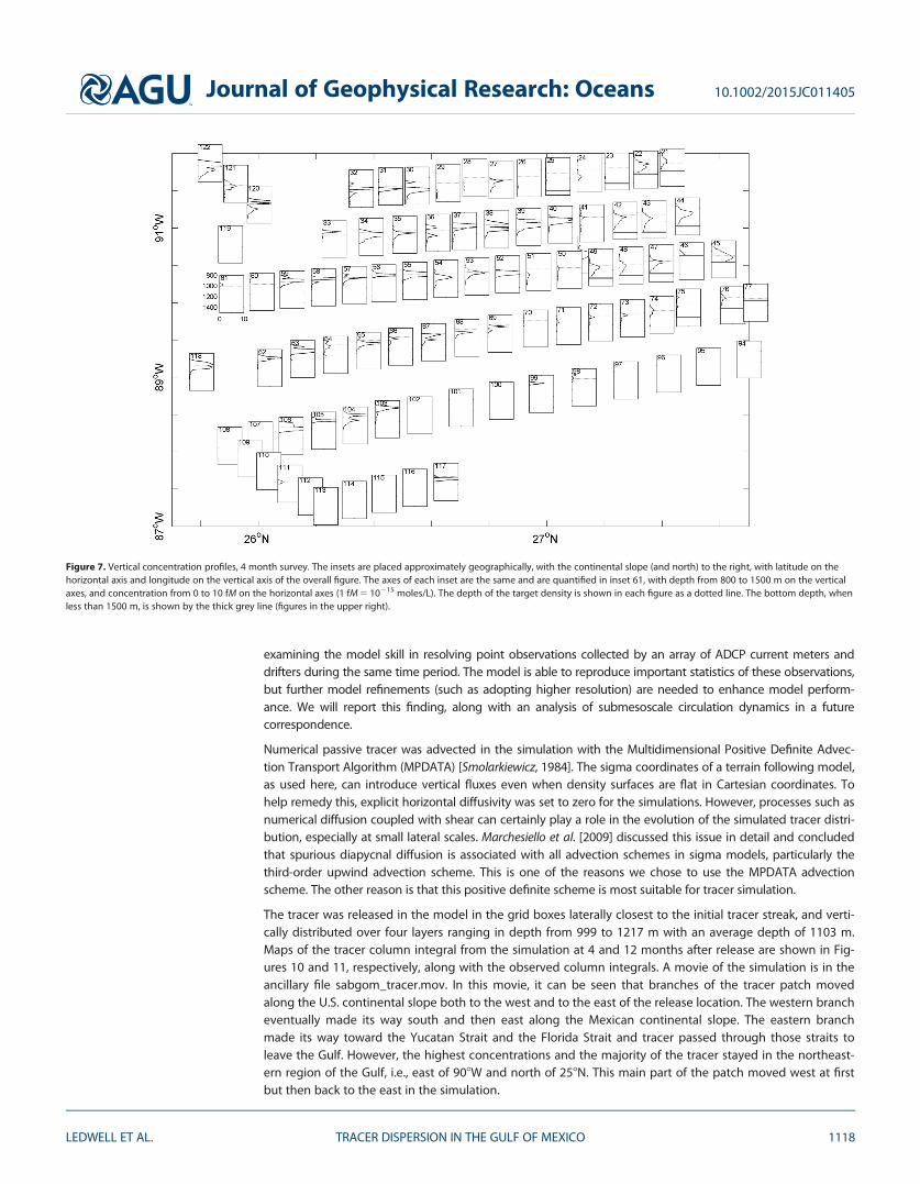
Individual vertical profiles of the tracer showed great variety (Figure 7). Profiles near the continental slopewere relatively simple in shape but were generally broader than the often multipeaked profiles found in theinterior. Multiple peaks indicate interleaving of low tracer water with high tracer water, a process which islikely at the edges of the tracer patch or at the edges of streaks within the tracer patch. An average overmany profiles, in density space, removes most of this effect, as will be seen in section 4.

The background color in Figure 4 is a map of the tracer constructed with objective analysis (or Kriging)based on the station data and using the covariance function shown in Figure 15. This map is highlysmoothed, masking the streakiness discussed in sections 4 and 5. The map accounts for 71% of the tracerreleased. Figure 4 shows tracer was very likely beyond the region surveyed, especially to the east and south.Also, our sampling may have missed high concentrations within the region surveyed due to streakiness(section 4).

2.5. Twelve Month SurveyThe tracer field was surveyed again in August 2013, approximately12 months after the release (Figure 8),from R/V Pelican using a CTD/Rosette system with 12 L Niskin bottles. Tracer profiles were found to berather smooth and the density range occupied by the tracer was found early to be predictable (Figure 9)and so only 12–14 of the Niskin bottles were tripped in the layer apparently occupied by the tracer. Theothers were used for sampling salinity and other constituents over the full water depth in order to add tothe rather scanty hydrographic database of the deep Gulf. Analysis of these more general geochemical datamust await a future communication.

Figure 3. Vertical concentration profiles from the integrating samplers during the initial survey. The cast number is indicated.



The samples were analyzed on board with the GC/ECD as described above. The volume of water spargedwas increased to 655 mL. For Stations 1–11, concentration uncertainties for the GC were again nearly 0.1 fM(1 standard deviation). After Station 11 concentration uncertainties were lowered to approximately 0.02 fMby eliminating noise with extensive baking of the GC detector and associated tubing.

Stations were widespread, although the ship time available did not allow a complete survey. Eddy ‘‘A’’ bythis time had weakened and moved west to about 268N, 958W where concentrations were low. Very littletracer was found within the Mexican EEZ (Figure 8). High concentrations were still found in the north alongthe slope, as for the 4 month survey, and were also found in the east. Again, a highly smoothed objectivemap of the tracer is shown in the background in Figure 8. The fraction of tracer represented in the map is53% of the amount released. This shortfall is discussed in section 4.

3. NumericalSimulation

Numerical simulations of theGulf circulation have been acontinuous community effortsince the late 1970s. Variouscirculation aspects in theGulf have been examinedusing models with different

Figure 4. Four month survey map. The circles along the black cruise track are colored according to the column integral of tracer found,with selected stations numbered for reference. The diffuse white to red colored background is a highly smoothed objective map based onthese station data (see text). Column integrals along transects labeled 1–5 at their northern ends are plotted in Figure 6. The abscissa andordinate are longitude (8W) and latitude (8N). Isobaths are plotted in blue every 500 m, deepening toward the south. The southern tip ofthe Louisiana coastline is barely visible in green near 298N, 89.48W. The Deepwater Horizon site (DWH) is at the black dot in the northeastcorner. The red box near 288N, 898W, delimits the map of the injection, shown here as a red line, and initial sampling shown in Figure 1.The mooring locations for the GISR experiment are shown as red asterisks. The serpentine line made of black dots is the trajectory ofRAFOS float 1215, released with the tracer and shown in detail in Figure 5. Sea surface height on 16 December 2012 is contoured in greyat 5 cm intervals, with negative contours dashed. ‘‘A’’ labels a prominent anticyclonic eddy, and ‘‘B’’ and ‘‘C’’ label weaker cyclonic and anti-cyclonic eddies, respectively. The tip of the Loop Current is in the southeast corner. Analyzed altimetry data are from the Colorado Centerfor Astrodynamics Research, and are viewable at the site http://eddy.colorado.edu/ccar/data_viewer/index.

Table 3. GC/ECD Analysis Operating Parameters

Precolumn 0.1 m long 3 0.83 mm ID SS Molecular Sieve 5A, 80/100 meshMain columns First: 1.2 m 3 0.83 mm ID SS Unibeads 2S

Second: 1.8 m 3 0.83 mm ID SS, Carbograph, 1% AT1000Column temperature 708C; precolumn heated to 958C during backflushCarrier UHP nitrogen at 25–30 mL/minGC Shimadzu GC8A with Electron Capture DetectorDetector temperature 3308CDetector current 2.0 nACold trap Unibeads 2S at 260 to 2708CSparge volume 260 mL (655 mL for the 12 month survey)Sparge flow UHP nitrogen at 150 mL/min for 4 min



http://eddy.colorado.edu/ccar/data_viewer/index

complexity and realism, includingtwo-layer and reduced gravity mod-els [e.g., Hurlburt and Thompson,1980] in the early stages and realistic,three-dimensional primitive equationbarotropic and baroclinic models inlast two decades [e.g., Oey, 1996;Morey et al., 2005; Chassignet et al.,2009; Halliwell et al., 2014, amongmany others]. In this study, the dis-persion of the tracer was simulatedwith the SABGOM circulation model.The model is described in detail else-where [Hyun and He, 2010; Xue et al.,2013, 2015]. Briefly, it is based on theRegional Ocean Modeling System(ROMS) [Shchepetkin and McWilliams,2005; Haidvogel et al., 2008] with hor-izontal resolution of approximately5 km, and with 36 vertical levels. Con-ditions at the open boundaries arefrom the 1/128 daily North AtlanticHybrid Coordinate Ocean Model(HYCOM/NCODA) [Chassignet et al.,2007], superimposed with eightmajor tidal harmonics derived from aregional tidal solution using the Ore-

gon State University Tidal Data Inversion Software (OTIS) [Egbert and Erofeeva, 2002]. Surface stress andbuoyancy forcing was from the 3 hourly, 32 km resolution, North American Regional Reanalysis (NARR,http://www.esrl.noaa.gov/psd/). The method of Mellor and Yamada [1982] was used to compute verticalturbulent mixing. Harmonic horizontal viscosity with a constant value of 100 m2 s21, and the quadraticdrag formulation with a drag coefficient of 3 3 1023 for the bottom friction specification were adopted.

Temperature and salinity wererelaxed to HYCOM/NCODA watermass fields with a 30 day timescale. This procedure allows themodel to evolve according to itsown high-resolution dynamics,while incorporating the low-frequency HYCOM model predic-tion that assimilates routine sat-ellite surface temperature, seasurface height, and available sub-surface hydrographic observa-tions. Extensive model-datavalidations have shown that SAB-GOM provides a realistic circula-tion hindcast in terms ofresolving mesoscale processes inthe Gulf, such as shelf circulation,the Loop Current, and Loop Cur-rent eddy dynamics [Hyun andHe, 2010; Xue et al., 2013, 2015;North et al., 2011, 2015]. We are

Figure 5. RAFOS 1215 trajectory. Deployment was at the NE end, during the injec-tion on 28 July 2012. Three fixes a day were obtained (dots). The excursion to theNW two thirds of the way through the trajectory started on 29 August, shortly afterlandfall of Hurricane Isaac on the Louisiana coast. During this excursion, the floathit the bottom on 1 September and apparently was damaged, because the pres-sure record indicated that after this time the float was hopping along the bottom.

Figure 6. Tracer column integral along transects 1–5 indicated in Figure 4. Distance ismeasured from the northernmost station.



http://www.esrl.noaa.gov/psd

examining the model skill in resolving point observations collected by an array of ADCP current meters anddrifters during the same time period. The model is able to reproduce important statistics of these observations,but further model refinements (such as adopting higher resolution) are needed to enhance model perform-ance. We will report this finding, along with an analysis of submesoscale circulation dynamics in a futurecorrespondence.

Numerical passive tracer was advected in the simulation with the Multidimensional Positive Definite Advec-tion Transport Algorithm (MPDATA) [Smolarkiewicz, 1984]. The sigma coordinates of a terrain following model,as used here, can introduce vertical fluxes even when density surfaces are flat in Cartesian coordinates. Tohelp remedy this, explicit horizontal diffusivity was set to zero for the simulations. However, processes such asnumerical diffusion coupled with shear can certainly play a role in the evolution of the simulated tracer distri-bution, especially at small lateral scales. Marchesiello et al. [2009] discussed this issue in detail and concludedthat spurious diapycnal diffusion is associated with all advection schemes in sigma models, particularly thethird-order upwind advection scheme. This is one of the reasons we chose to use the MPDATA advectionscheme. The other reason is that this positive definite scheme is most suitable for tracer simulation.

The tracer was released in the model in the grid boxes laterally closest to the initial tracer streak, and verti-cally distributed over four layers ranging in depth from 999 to 1217 m with an average depth of 1103 m.Maps of the tracer column integral from the simulation at 4 and 12 months after release are shown in Fig-ures 10 and 11, respectively, along with the observed column integrals. A movie of the simulation is in theancillary file sabgom_tracer.mov. In this movie, it can be seen that branches of the tracer patch movedalong the U.S. continental slope both to the west and to the east of the release location. The western brancheventually made its way south and then east along the Mexican continental slope. The eastern branchmade its way toward the Yucatan Strait and the Florida Strait and tracer passed through those straits toleave the Gulf. However, the highest concentrations and the majority of the tracer stayed in the northeast-ern region of the Gulf, i.e., east of 908W and north of 258N. This main part of the patch moved west at firstbut then back to the east in the simulation.

Figure 7. Vertical concentration profiles, 4 month survey. The insets are placed approximately geographically, with the continental slope (and north) to the right, with latitude on thehorizontal axis and longitude on the vertical axis of the overall figure. The axes of each inset are the same and are quantified in inset 61, with depth from 800 to 1500 m on the verticalaxes, and concentration from 0 to 10 fM on the horizontal axes (1 fM 5 10215 moles/L). The depth of the target density is shown in each figure as a dotted line. The bottom depth, whenless than 1500 m, is shown by the thick grey line (figures in the upper right).



As might be expected, due to propagation of model errors over such long times and the patchy nature ofthe tracer distribution, there are many differences in a point by point comparison between simulated andobserved tracer fields. Displacements of this scale could have a myriad of origins, but one likely source isenergetic mesoscale meanders and eddies within the gulf. These motions exist in the present physicalmodel (grid spacing of 5 km) but cannot be deterministically replicated. Broadly speaking, at 4 months thesimulated tracer seems to lie to the east and the north of the observed tracer (Figure 10). At 12 months, thesimulated tracer may again be more concentrated to the east of observed tracer. Particularly notable is thatthe simulation did not capture the relatively high tracer concentrations observed along the continentalslope near 908W (Figure 11). However, as will be discussed in the next section, some important statistics ofthe simulated tracer distribution do match the observations. As will also be seen, details that are resolvablein the simulation but not in the sparsely spaced observations, help interpret the latter.

4. Analysis

4.1. Diapycnal Diffusivity—First 4 MonthsDiapycnal diffusivities may be estimated from the progression of the distribution of the tracer in densityspace with time. There are two confounding difficulties with the current experiment. A relatively minor oneis that the diapycnal distribution at densities greater than the target density of the release was not wellbounded (Figure 3), due to the short length of the lower part of the sampling array. This difficulty turns outto be minor because the least squares procedure described below calls for virtually no tracer deeper thanthe range sampled during the initial survey, though it is free to call for as much tracer as needed there tominimize the cost function.

Figure 8. Twelve month survey map. The circles along the black cruise track are colored according to the column integral of tracer found,with selected stations numbered for reference. The diffuse white to red colored background is a highly smoothed objective map based onthese station data (see text). Isobaths are plotted in blue every 500 m, and the coastline is green.



The other confounding difficulty, which however adds interest to the experiment, is that mixing was appa-rently much greater near the continental slope than away from it. The tracer release approach is not a verysharp tool in differentiating between boundary mixing and interior mixing because one cannot control or

Figure 9. Vertical concentration profiles, 12 month survey. Some closely spaced profiles are omitted for clarity. Profiles 1–11 are not plotted due to GC noise. The insets are placedapproximately geographically. The axes of each inset are the same and are quantified in inset 43, with depth from 800 to 1500 m on the vertical axes, and concentration from 0 to 1.5 fMon the horizontal axes. The depth of the target density is shown in each figure as a dotted line. The bottom depth, when less than 1500 m, is shown by the thick gray line (figures alongthe northwest edge).

Figure 10. Numerical simulation of the tracer column integral 4 months after release (red) superposed on the observed column integral from thestations occupied at 4 months (circles filled with red from the same palette). Isobaths are shown every 500 m. Sea surface height anomaly con-tours are shown in grey at 5 cm intervals, solid for positive anomalies, dashed for negative. Eddies A, B, and C and the Loop Current are indicated.



know the amount of time the tracer has spent in the respective regions. However, the tracer measurementsdo allow useful limits to be placed on the diffusivities in the two regions.

To this end, the stations have been divided into two groups, a ‘‘boundary’’ group comprising all the stationsshoreward of the 1500 m isobath, and an ‘‘interior’’ group comprising those stations seaward of this isobath.The boundary stations are those in Figure 7 for which the bottom appears on the profile subplots as a thickgray band. The choice of this dividing isobath is somewhat arbitrary, but it does separate the simple broadpeaks near the slope from the narrower interior peaks. The means of these two groups (Figure 12) werecomputed as a function of density and then converted to depth through the mean depth/density relationfor the interior stations, shown in Figure 13. The mean boundary profile is much broader than the meaninterior profile, in this common coordinate, especially in the deep wing of the profile, implying that mixingwas enhanced near the boundary. Discontinuities in the boundary profile are due to profiles dropping outof the mean because of the presence of the bottom.

A diapycnal diffusivity of 1.3 3 1024 m2/s is estimated by applying a 1-D diffusion model to the changefrom the initial mean profile to the mean interior profile for the 4 month survey, following the method ofLWL (Figure 12). The least squares procedure of this model selects concentrations in the initial deep tail thatfall off rapidly at depths greater than 40 m below the target density surface, the limit of the observations.As noted earlier, the implication is that the observed deep tracer at 4 months does not indicate that verymuch tracer resided in the unsampled region below 240 m during the initial survey.

Application of the same 1-D diffusion model to the evolution from the initial mean profile to the meanboundary profile gave an estimate of the diffusivity for the boundary region of 4 3 1024 m2/s, though witha much poorer fit than for the mean interior profile (Figure 12). The interpretation of this result is notstraightforward, because: the diapycnal diffusivity no doubt depends on distance from the boundary; thecategorization of ‘‘boundary’’ is arbitrary; and how close to the boundary the tracer in each profile had beensince the release is unknown. The difference between the interior and boundary result for the diffusivity isstrong evidence, however, for significant enhancement of mixing over the slope.

The same caveats as above apply to the diffusivity of 1.3 3 1024 m2/s inferred from the mean interior pro-file. This is not to be taken as the diffusivity in the interior, because most of the tracer probably spent sometime in the boundary region. The evolution from 4 to 12 months, to be discussed next, gives a much smaller

Figure 11. Numerical simulation of the tracer column integral 12 months after release (red) superposed on the observed column integralfrom the stations occupied at 12 months (circles filled with red from the same palette). Isobaths are shown every 500 m (blue); the coast isshown in black.



diffusivity for the interior for thattime period. Because of theambiguity in where the tracerhas been, we do not assign errorbars to the diffusivities inferredfor this first time period.

4.2. Diapycnal Diffusivity—Four to Twelve MonthsThe mean of all the profiles fromthe survey in August 2013, 12months after release, was almostindistinguishable from the meaninterior profile at 4 months (Fig-ure 14; the 4 month profile wasshifted up by 10 m, assuming aCTD calibration shift). Applica-tion of the 1-D diffusion modelof LWL yields a diapycnal diffu-sivity of (0.15 6 0.05) 3 1024

m2/s, an order of magnitudesmaller than found for theperiod between the initial surveyand the 4 month survey, andsimilar to values found fromtracer release experiments in theinterior of the open ocean [Led-well et al., 2011; LWL]. Inclusionof a vertical gradient in the dia-pycnal diffusivity, which isallowed by the method, doesnot improve the fit significantly.The result for the diffusivity isnot sensitive to the shift of 10 mthat was applied to the 4 monthmean profile, but the cost func-tion is reduced by this shift.Uncertainties reported here aresubjective estimates from thebehavior of the cost functionused in the least squares proce-dure, and assessment of the dif-ference between observed andmodeled mean profiles.

4.3. Spatial AutocorrelationMapping a tracer cloud for anexperiment such as ours is verymuch like mapping mineral veinsin the mining industry. Hence,we borrow statistical techniquesfrom that field, and in particularthe variogram [e.g., Journel andHuijbregts, 1978]. A normalizedspatial covariance based on the

Figure 12. Initial and 4 month mean vertical profiles. Height is relative to the target isopyc-nal surface. The dashed black curve is the mean of the individual profiles from the initialsurvey, 5–12 days after release, multiplied by 0.004 to graph it with the other profiles. Thered and blue curves are the mean of the interior and boundary profiles, respectively, fromthe 4 month survey. The black dotted and dashed red curves are the least squares fit tothe initial profile and the 4 month interior profile, respectively, from the 1-D diffusionmodel, with diffusivity 1.3 3 1024 m2/s. The dashed blue curve is the least squares fit fromthe 1-D model for the boundary profile with diffusivity 4 3 1024 m2/s.

Figure 13. Mean density profile for the interior stations from the 4 month survey. The refer-ence pressure for potential density is 1000 dbar. This curve is used to convert all of themean profiles in density space to mean profiles in height above the target surface.



variogram, which we shall callthe spatial autocorrelation, is:

Ak � 12

XN

m51

XNkm

n51Im2Inð Þ2

� �

XN

m51

XNkm

n51I2m1I2

n

� ��

(1)

where N is the number of sta-tions, Im is the column integralof tracer at station m, and thesums are over all pairs of sta-tions separated by a distancer in distance bin k defined byrk� r< rk 1 Dr, where Dr is thebin size. That is,

PNkm

n51 is a sumover those stations whose dis-tance from station m is in thekth bin. To maintain symmetryin (1), all pairs are counted twicein both the numerator and thedenominator. Ak takes on thevalue 1 at distance 0, and tendsto decrease with increasing dis-tance, but is always positive.Pairs whose members are bothzero do not contribute to thesums at all, which is an advant-age over the spatial autocorrela-tion defined in LWL.

This spatial autocorrelation is shown in Figure 15 for the observations and, in the case of the 4 and 12month surveys, for the SABGOM simulation sampled at the same locations as the observations. Error barswere estimated by the jackknife method [Effron and Gong, 1983]. The magnitude of the abrupt drop in theautocorrelation between 1 at zero distance and the value in the first distance bin gives coarse informationon the magnitude of unresolved small-scale features of the tracer patch, such as filament width. The muchgreater length scale of the drop beyond the first bin seems to be on the order of the overall size of thetracer patch rather than of details within it.

Figure 15 includes, for the 4 and 12 month surveys, exponential fits to the spatial autocorrelation that wereused in making the smooth color maps of the tracer field in Figures 4 and 8, using the method of objectiveanalysis [Bretherton et al., 1976], or, equivalently, simple Krigging with a nugget effect [e.g., Journel and Huij-bregts, 1978]. These maps do not at all capture the interesting filamentation that is certainly there, as exem-plified by the numerical simulations discussed in the next subsection.

4.4. StreakinessThe maps of Figures 10 and 11 show the tracer in the SABGOM numerical simulation to be distributed inbroad streaks created by the stirring of the eddy field. The same phenomenon has been seen in many pastsimulations of tracer dispersion in the ocean [e.g., Haidvogel and Keffer, 1984; Sundermeyer and Price, 1998; Leeet al., 2009; Tulloch et al., 2014]. This behavior was described elegantly by Garrett [1983]. The actual tracer dis-tribution was presumably arranged in streaks qualitatively similar to those in the simulation, but the resolutionand coverage of the sampling at 4 and 12 months were not at all adequate to reveal streaks directly.

As noted in section 2, the initial survey found the tracer distributed in features a few km across (Figure 2). Itappears that individual streaks were resolved by the 50 chamber sampler, although spatial aliasing of

Figure 14. Mean of the interior profiles at 4 months, shifted up 10 m (dashed black curve),of all the profiles at 12 months (solid black), and least squares fit from the model for the 4month mean (dotted blue) and the 12 month mean (dash-dotted magenta). Height is rela-tive to the target isopycnal surface.



streaks at smaller scales than resolved is always likely. The spatial autocorrelation drops rapidly with dis-tance, falling to 0.65 in the first bin, centered at 0.5 km, and falling to less than 0.2 beyond 4 km (Figure15a). It is clear that at this early time in the experiment sampling with a towed system rather than spot sam-pling with vertical CTD/Rosette casts was advantageous, if not absolutely necessary.

By the time of the 4 month cruise, the tracer distribution seemed to be coherent over scales of tens of kilo-meters (Figure 6), so that sampling by CTD/Rosette was effective. The autocorrelation again drops to 0.65 inthe first bin, which, however, is now 20 km wide, and drops to around 0.2 beyond 250 km, the peak withlarge error bars at 290 km notwithstanding (Figure 15b). The autocorrelation for the SABGOM simulation atthis time drops only to 0.9 in the first bin, versus 0.65 for the real tracer, suggesting that the real tracerstreaks were narrower than those evident in the simulation in Figure 10. The two autocorrelations convergenear 250 km, suggesting that the overall length scales of the observed and simulated patches were similar.

At 12 months, the autocorrelation for both the observed and simulated tracer patches drops to around 0.85in the first 80 km wide bin (Figure 15c). Filaments are much broader, or are on their way to merger by thismeasure, compared with 4 months, and the variability at these scales seen in the simulation (Figure 11) isperhaps a guide to scales of variability for the actual tracer. Beyond the first distance bin, however, the auto-correlation falls off much faster for the observations than for the simulation (Figure 15c). This is perhapsdue to the simulated tracer more nearly filling the Gulf than appears to be the case in the observations: col-umn integrals in the southwest half of the Gulf were 10–20% of the maximum values in the simulated field(Figure 11), while the sparse sampling of the survey found virtually no tracer in this region.

Figure 15. Spatial autocorrelation Ak of concentration at the 50 chamber sampler (a) for the initial survey 5–12 days after injection, (b) for the column integral of tracer for the 4-monthsurvey for the observations (solid), and (c) for the simulation sampled at the same locations as for the 12-month survey (dashed), all from equation (1). The same function for the tracerrelease in the North Atlantic (LWL) at 12 months after release is plotted as a dash-dotted line in Figure 15c. The dotted lines in Figures 15b and 15c are the autocorrelation functionsused in the color tracer maps in Figures 4 and 8, respectively.



4.5. Mass BudgetsAs noted earlier, the fraction of tracer integrated over the objective maps of Figures 4 and 8 for the 4 and12 month surveys was 72% and 53%, respectively. There is considerable uncertainty in the integral of mapslike these, but by any means of integration there appear to be shortfalls of this order in the surveys. Lossover the 800 m deep sill in Florida Strait seems very unlikely. Loss through the Yucatan Channel between 4and 12 months is possible, however, as shown by moored current meter arrays [Ochoa et al., 2001; Bungeet al., 2002; Sheinbaum et al., 2002; Candela et al., 2002; Badan et al., 2005; Rivas et al., 2005]. Sturges [2005]has shown a three-layer system below 800 m, with water flowing into the Gulf between 800 and 1100 mand between about 1900 m and the bottom, but flowing out of the Gulf to the south between 1100 and1900 m. Observations indicate an outward volume flow of about 1 Sv (1 3 106 m3/s) [Rivas et al., 2005; Sturges,2005], while circulation models suggest a somewhat larger flow of order 3 Sv, with considerable variability[Cherubin et al., 2005]. In the SABGOM simulation, only 2% of the tracer leaves the Gulf by this route by 12months, with most of the escape occurring between 4 and 12 months. We can only speculate on how muchof the real tracer passed into the Caribbean, but it does not seem that this route can account for the missingtracer.

Part of the explanation for the shortfalls in the mass integrals lies in the spatial autocorrelations discussedabove, the streakiness of the tracer making it harder to find. Also, high concentrations found around thegeographical limits of the 4 month survey indicated that we missed tracer beyond these boundaries. At 12months, the observations found no tracer in the southwest half of the Gulf, but there is a large unsampledarea there, and in fact there are large spaces between all the sampling lines. Hence, perhaps the best expla-nation for the shortfall of the 12 month survey is that much of the tracer was far from the sparsely spacedtrack lines.

4.6. Distribution of ConcentrationsA histogram of the concentrations found during the initial survey in the 50 chamber sampler is shown inFigure 16a, with a bin size of 2.5 pM (1 pM 5 10212 moles/L). The concentrations are actually means alongthe approximately 600 m tow segments over which the syringes filled. Since the sampling sled was towednear the isopycnal surface of the release, these concentrations would have been near the maximum fortheir location. Concentrations above and below the sled would have decreased with vertical distanceapproximately in proportion to the average profile shown in Figure 12, the standard deviation of which isabout 15 m. The most frequently encountered concentration was in the first histogram bin of 0–2.5 pM,since most of the area surveyed was devoid of tracer, and in fact the concentration in 105 of the 137 sam-ples in that bin were zero. The histogram falls abruptly in the next four bins, to zero between 12.5 and 17.5pM, with a few samples found in outlying bins between 17.5 and 27.5 pM. The largest concentrationencountered was just slightly over 25 pM.

Histograms of the maximum concentration found at each station during the 4 and 12 month surveys areshown in Figures 16b and 16c, respectively. These concentrations are for spot samples captured with Niskinbottles, rather than averages along a tow track. Again, the maximum number of samples was in the firstbin, and fell to zero after several bins, with a few concentrations in outlying bins. The maximum concentra-tion at 4 months was 45 fM and at 12 months was 2.5 fM. With time, the peak in number in the first binbecame less pronounced compared with the other bins, i.e., from initial to 4 to 12 month survey, as thetracer became more evenly distributed within the surveyed areas. These maximum concentrations werefound near the target isopycnal surface. The distribution at other levels can be estimated from these histo-grams, but with the concentration scale diminished following the approximately Gaussian curves describingthe mean vertical profiles, shown in Figures 12 and 14.

Because the vertical resolution of the SABGOM model is coarse compared with the narrow vertical width ofthe tracer distribution, it is best to compare column integrals rather than concentrations in the simulationwith observations, as done in the maps of Figures 10 and 11. Figure 17 compares histograms of theobserved column integrals at the stations of the 4 and 12 month surveys with histograms of simulated col-umn integrals sampled at the same locations. The distributions of column integrals appear to be quite simi-lar to one another. Perhaps the most important difference is that for the 12 month survey the first bin in thesimulation is less populated than in the observations. That is, there are relatively fewer low concentrations



because the tracer is spread more homogeneously in the simulation than in the observations. This relativehomogenization was suggested by the spatial autocorrelation.

5. Discussion

5.1. Boundary MixingIn section 4, we showed that diapycnal dispersion of the tracer observed 4 months after the release wassignificantly greater for the profiles near the northern continental slope of the Gulf than in the interior. At12 months, the diapycnal distribution of the tracer was not much changed from the mean interior distri-bution at 4 months, implying a diffusivity of 0.15 3 1024 m2/s, of order 10 times smaller than for the ear-lier period. We take these results as strong evidence that diapycnal mixing was greatly enhanced over theslope, since the tracer most likely spent more time over the slope during the first period than during thesecond period.

Time dependence, as well as this spatial dependence, is likely to have played a role, however. HurricaneIsaac passed directly over the site of the experiment about 1 month after the tracer release. The bottom-most moored current meters at the mooring sites indicated in Figure 4 show that more than 20% of theenergy dissipation along the slope for the whole 12 month period probably occurred in the aftermath ofthis hurricane. Still, about as much energy was dissipated in the time interval between 4 and 12 months asduring the first 4 months. By this measure, we would expect about the same amount of mixing in the two

Figure 16. Histograms of maximum concentrations for the three surveys: (a) in the syringes in the system towed near the isopycnal surface of the release, in pM; (b, c) at the stations forthe 4 and 12 month survey, respectively, in fM.



periods if boundary mixing played aminor role, i.e., about the same increasein mean squared diapycnal dispersion ofthe tracer. Thus, the evidence for greatenhancement near the boundaries iscompelling.

We summarized many of the mechanismsforcing bottom currents along the slopein section 1. The dominant mechanismfor our time period seems to be windforcing, as discussed above, but Loop Cur-rent eddies and topographic Rossbywaves propagating along the slope nodoubt also played a role. Currents alongthe northern slope pass over a bottomthat is corrugated with canyons andpimpled with salt domes (Figure 18). Inwork under way, K. Polzin and othersspeculate that form drag acting on flowover these features generates turbulentenergy that is dissipated in a relativelyshallow, but stratified, boundary layer,resulting in the strong mixing that wehave observed.

The diapycnal diffusivity of 0.15 3 1024

m2/s, found for the interior between 4 and12 months, is typical of open ocean con-ditions. For example, the value from the30 month long tracer release experimentin the eastern subtropical gyre of theNorth Atlantic at 300–400 m depth was0.17 3 1024 m2/s (LWL). The value foundin the southeast Pacific sector of the Ant-

arctic Circumpolar Current, a very energetic region, was 0.13 3 1024 m2/s near 1500 m depth [Ledwell et al.,2011]. The diffusivity inferred from dissipation rates of turbulent kinetic energy at all depths, i.e., independ-ent of buoyancy frequency, in the background internal wavefield at midlatitudes is even smaller, at approxi-mately 0.05 3 1024 m2/s [Gregg, 1989; Polzin et al., 1995]. Thus, conditions for turbulent mixing in theinterior of the Gulf may be quite similar to those in the interior of the open ocean, far from topography.

5.2. Lateral Dispersion and HomogenizationRates of lateral stirring and mixing and the consequent dilution of peak concentrations are of importance tothe ecology of the middepth Gulf because of the potential for release of pollutants from drilling activities aswell as the prevalence of natural hydrocarbon seeps. Lateral dispersion along isopycnal surfaces is farmore effective at spreading and diluting a tracer than diapycnal dispersion, though the latter may play animportant role in lateral dispersion through the process of shear dispersion at small scales. We estimatefrom the concentrations found that the area covered by the tracer at the time of the initial survey was about50 km2. After 1 year, the tracer was found spread over a good fraction of the Gulf, whose area at 1100 m isapproximately 600,000 km2. The peak concentration fell correspondingly, from 2.6 3 10211 to 2.5 3 10215

moles/kg. The mechanism for this huge dilution factor is stirring of the tracer by the shears and strains ofboundary currents, mesoscale eddies, and a poorly understood cascade of smaller-scale motions, and thenby the shear-induced turbulent events at submeter scales, and finally by molecular diffusion at scales of acentimeter or so.

Figure 17. Histograms of the column integral observed (left) at the 4 and 12month stations and (right) at those stations in the numerical simulation. Thevertical axes give the number of stations in each bin. Note that the range ofthe horizontal axis is 10 times smaller at 12 months than at 4 months due todispersion of the tracer.



Homogenization is a competitionbetween stirring at small scales, tend-ing to fill in the general area occupiedby the tracer, against stirring at largerscales, tending to disperse the tracerand enlarge the overall area to be filledin [e.g., Garrett, 1983]. In the openocean conditions of the North AtlanticTracer Release Experiment (NATRE),tracer streaks 5 months after releasewere of order 10 km across, but sepa-rated by many tens of km, renderingthe tracer very hard to find. One possi-ble explanation for the relative homo-geneity of the present tracer patch at4 months is that it had been held closeenough to the boundary for a longenough time to be spread into a broadband before it was carried away fromthe slope. It is also likely that sheardispersion associated with greatlyenhanced diapycnal mixing over theslope helped broaden tracer streaks.Only after 12 months had the lengthscales of the spatial autocorrelation inthe North Atlantic become as greatas those in the present experimentat 4 months (compare Figures 15band 15c).

An interesting question is the extent to which the tracer moved upward across the continental slopetoward the shelf, shoreward of our stations. What evidence we have does not indicate such upwelling.Isopycnal surfaces consistently deepened toward the slope along the tow tracks shown in Figure 1.Downward dipping isopycnals are consistent with downwelling bottom Ekman currents resulting fromsouthwestward flow along the slope. Also, our boundary stations during the surveys at 4 and 12 monthsare generally within 30 km of the grounding lines of the isopycnal surfaces occupied by the tracer. Weestimate from our results on lateral dispersion that the time for communication between these ground-ing lines and the stations is a month or two, so that the boundary profiles seen in Figures 7 and 9and the mean boundary profile in Figure 12 may well be representative of what tracer has made itup the slope.

5.3. Peak ConcentrationsThe maximum of all the concentrations found during each survey is shown in Figure 19. The concentrationin the initial plume of the injection sled is estimated to have been about 9 3 1027 moles/kg (the first pointshown in Figure 19). The maximum concentrations actually observed during the three surveys are shown asthe last three points lying on a straight line in Figure 19. These suggest a t22.5 dependence, where t is thetime since release.

This last result is reminiscent of the diffusion diagrams of Okubo [1971], who found that the area of dyepatches released in the upper ocean in coastal and shelf areas grew like t2.34. Aside from the fact that verti-cal mixing in the present experiment would add another 0.5 to the exponent, this apparent agreement con-ceals several aspects of dispersion in the present experiment that are absent in the experimentssynthesized by Okubo. First of all, there may be enhanced dispersion near the slope due to cross-slopeshear in the along-slope currents coupled with cross-slope diffusivity. Then, as part of the patch leaves theboundary region, it would be stirred by eddies into filaments with an exponential growth in the along-filament direction, and perhaps a cross filament scale that is not growing at all or is even shrinking because

Figure 18. Example of the complex bathymetry of the continental slope along thenorthern Gulf of Mexico, from the region at which high tracer concentrations werefound. Depth is in meters; the view is from the southeast. The map grid is 1.63 km3 1.83 km (zonal 3 meridional). Bathymetry data are from the NOAA NationalGeophysical Data Center, U.S. Coastal Relief Model, available at the web site http://www.ngdc.noaa.gov/mgg/coastal/crm.html.





of convergence in the cross-filamentdirection [e.g., Garrett, 1983]. Thus,several processes, some no doubt notmentioned here, go into the trend inFigure 19. Nevertheless, the order ofmagnitude of the dilution over thevarious time scales of the experiment,i.e., 10 days or so for the initial survey,and then 4 and 12 months for thesubsequent surveys, provide usefulphenomenology for dispersion nearthe continental slope and interior ofthe Gulf: we see a time dependenceof the maximum concentration oft22.5 for time t between 10 days and12 months after the release.

A power law dependence of peak con-centration stronger than 21.5 impliesthat lateral dispersion was ‘‘superdiffu-sive,’’ that is exhibiting a stronger timedependence than Fickian diffusion.Super diffusive dispersion of surfacedrifters was also found by LaCasce andOhlmann [2003] for the surface watersof the northern shelf and slope of theGulf, though they were able to discernperiods of exponential growth andpower law growth from their detailed

time series of many pairs and triplets of drifters. Our study is of stirring at 1100 m, where kinetic energy is muchlower than near the surface, and Eulerian time scales appear to be rather different [see, e.g., Hamilton, 1990;Hamilton and Lugo-Fernandez, 2001]. Nevertheless, superdiffusive dispersion seems to be more the norm thanthe exception in the Gulf at least at scales below the mesoscale.

6. Summary

The following conclusions may be drawn from the experiment:

1. Diapycnal mixing at middepth in the northern Gulf of Mexico is much greater near thecontinental slope than in the interior, where it is approximately 0.15 3 1024 m2/s, a value typical of theopen ocean.

2. Homogenization of a tracer released near the slope proceeds faster than in the open ocean; fast enoughto sample effectively with discrete stations after a few months.

3. Concentrations of a tracer released along the slope at middepth fell by a factor of approximately 200 in aperiod of 10 days or so, by a factor of 105 over 4 months, and by another factor of 10 over the next 8months.

Understanding the physics behind these conclusions will benefit from past work, and especially from meas-urements made concurrently with the tracer experiment by the GISR mooring array, and from fine andmicrostructure profiles made as part of GISR. Analysis and interpretation of these data are under way. TheSABGOM numerical simulation was able to replicate important statistics of observed tracer and helpedinterpret the dispersion of the tracer, and especially the evolution of streakiness and of the concentrationdistribution. Conversely, the behavior of the tracer and its explanation in terms of forcing will help todevelop more advanced numerical schemes and next generation ocean models that could be used to bet-ter forecast the trajectories, concentrations, and the fate of substances released at depth in the Gulf ofMexico, either accidentally or naturally.

Figure 19. Maximum tracer concentration as a function of time. The point labeled‘‘Initial Plume (Est.)’’ is an estimate for the tracer concentration in the initial turbu-lent plume of the injection sled. The dashed line along the survey points indicatesa t22.5 power law.



ReferencesBadan, A., J. Candela, J. Sheinbaum, and J. Ochoa (2005), Upper-layer circulation in the approaches to Yucatan Channel, in Circulation in the

Gulf of Mexico: Observations and Models, Geophys. Monogr. Ser., vol. 161, edited by W. Sturges III and A. Lugo-Fernandez, pp. 57–69,AGU, Washington, D. C.

Banyte, D., T. Tanhua, M. Visbeck, D. W. R. Wallace, J. Karstensen, G. Krahmann, A. Schneider, L. Stramma, and M. Dengler (2012), Diapycnaldiffusivity at the upper boundary of the tropical North Atlantic oxygen minimum zone, J. Geophys. Res., 117, C09016, doi:10.1029/2011JC007762.

Boland, E. J. D., E. Shuckburgh, P. H. Haynes, J. R. Ledwell, M.-J. Messias, and A. J. Watson (2015), Determining a sub-mesoscale diffusivityusing a roughness measure applied to a tracer release experiment in the Southern Ocean, J. Phys. Oceanogr., 45, 1610–1631, doi:10.1175/JPO-D-14-0047.1.

Bretherton, F. P., R. E. Davis, and C. B. Fandry (1976), A technique for objective analysis and design of oceanographic experiments appliedto MODE-73, Deep Sea Res. Oceanogr. Abstr., 23(7), 559–582, doi:10.1016/0011-7471(76)90001-2.

Bunge, L., J. Ochoa, A. Badan, J. Candela, and J. Sheinbaum (2002), Deep flows in the Yucatan Channel and their relation to changes in theLoop Current extension, J. Geophys. Res., 107(C12), 3233, doi:10.1029/2001JC001256.

Camilli, R., C. M. Reddy, D. R. Yoerger, B. A. S. Van Mooy, M. V. Jakuba, J. Kinsey, C. P. McIntyre, S. P. Sylva, and J. V. Maloney (2010), Trackinghydrocarbon plume transport and biodegradation at Deepwater Horizon, Science, 330, 201–204, doi:10.1126/science.1195223.

Candela, J., J. Sheinbaum, J. Ochoa, and A. Badan (2002), The potential vorticity flux through the Yucatan Channel and the Loop Current inthe Gulf of Mexico, Geophys. Res. Lett., 29(22), 2059, doi:10.1029/2002GL015587.

Chassignet, E. P., H. E. Hurlburt, O. M. Smedstad, G. R. Halliwell, P. J. Hogan, A. J. Wallcraft, R. Baraille, and R. Bleck (2007), The HYCOM(hybrid coordinate ocean model) data assimilative system, J. Mar. Syst., 65, 60–83.

Chassignet, E. P., et al. (2009), U.S. GODAE: Global ocean prediction with the hybrid coordinate ocean model (HYCOM), Oceanography,22(3), 48–59.

Cherubin, L. M., W. Sturges, and E. P. Chassignet (2005), Deep flow variability in the vicinity of the Yucatan Straits from a high-resolutionnumerical simulation, J. Geophys. Res., 110, C04009, doi:10.1029/2004JC002280.

Egbert, G. D., and S. Y. Erofeeva (2002), Efficient inverse modeling of barotropic ocean tides, J. Atmos. Oceanic Technol., 19, 183–204, doi:10.1175/1520-0426(2002)019< 0183:EIMOBO>2.0.CO;2.

Effron, B., and G. Gong (1983), A leisurely look at the bootstrap, the jackknife, and cross-validation, Am. Stat., 37, 36–48.Garrett, C. (1983), On the initial streakiness of a dispersing tracer in two- and three-dimensional turbulence, Dyn. Atmos. Oceans, 7(4),

265–277, doi:10.1016/0377-0265(83)90008-8.Gregg, M. C. (1989), Scaling turbulent dissipation in the thermocline, J. Geophys. Res., 94(C7), 9689–9698.Haidvogel, D. B., and T. Keffer (1984), Tracer dispersal by mid-ocean mesoscale eddies, Part I. Ensemble statistics, Dyn. Atmos. Oceans, 8(1),

1–40, doi:10.1016/0377-0265(84)90002-2.Haidvogel, D. B., et al. (2008), Ocean forecasting in terrain-following coordinates: Formulation and skill assessment of the regional ocean

modeling system, J. Comput. Phys., 227, 3595–3624.Halliwell, G. R., Jr., A. Srinivasan, V. Kourafalou, H. Yang, D. Willey, M. Le Henaff, and R. Atlas (2014), Rigorous evaluation of a fraternal twin

ocean OSSE system in the open Gulf of Mexico, J. Atmos. Oceanic Technol., 31, 105–130, doi:10.1175/JTECH-D-13-00011.1.Hamilton, P. (1990), Deep currents in the Gulf of Mexico, J. Phys. Oceanogr., 20(7), 1087–1104, doi:10.1175/1520-0485(1990)020<1087:DCIT-

GO>2.0.CO;2.Hamilton, P. (2009), Topographic Rossby waves in the Gulf of Mexico, Prog. Oceanogr., 82(1), 1–31, doi:10.1016/j.pocean.2009.04.019.Hamilton, P., and T. N. Lee (2005), Eddies and jets over the slope of the northeast Gulf of Mexico, in Circulation in the Gulf of Mexico: Observa-

tions and Models, Geophys. Monogr. Ser., vol. 161, edited by W. Sturges III and A. Lugo-Fernandez, pp. 123–142, AGU, Washington, D. C.Hamilton, P., and A. Lugo-Fernandez (2001), Observations of high speed deep currents in the northern Gulf of Mexico, Geophys. Res. Lett.,

28(14), 2867–2870, doi:10.1029/2001GL013039.He, R., and R. H. Weisberg (2002), Tides on the West Florida Shelf, J. Phys. Oceanogr., 32(12), 3455–3473.Ho, D. T., J. R. Ledwell, and W. M. Smethie Jr. (2008), Use of SF5CF3 for ocean tracer release experiments, Geophys. Res. Lett., 35, L04602,

doi:10.1029/2007GL032799.Holtermann, P. L., L. Umlauf, T. Tanhua, O. Schmale, G. Rehder, and J. Waniek (2012), The Baltic Sea tracer release experiment: 1. Mixing

rates, J. Geophys. Res., 117, C01021, doi:10.1029/2011/JC007439.Hurlburt, H. E., and J. D. Thompson (1980), A numerical study of Loop Current intrusions and eddy shedding, J. Phys. Oceanogr., 10,

1611–1651.Hyun, H. H., and R. He (2010), Coastal upwelling in the South Atlantic Bight: A revisit of the 2003 cold event using long term observations

and model hindcast solutions, J. Mar. Syst., 83, 1–13, doi:10.1016/j.jmarsys.2010.05.014.Jaimes, B., and L. K. Shay (2010), Near-inertial wave wake of hurricanes Katrina and Rita over mesoscale oceanic eddies, J. Phys. Oceanogr.,

40, 1320–1337.Journel, A. G., and Ch. J. Huijbregts (1978), Mining Geostatistics, 600 pp., Academic, San Diego, Calif.Kantha, L. (2005), Barotropic tides in the Gulf of Mexico, in Circulation in the Gulf of Mexico: Observations and Models, Geophys. Monogr. Ser.,

vol. 161, edited by W. Sturges and A. Lugo-Fernandez, pp. 159–163, AGU, Washington, D. C.LaCasce, J. H., and C. Ohlmann (2003), Relative dispersion at the surface of the Gulf of Mexico, J. Mar. Res., 61, 285–312.Law, C. S., A. J. Watson, and M. I. Liddicoat (1994), Automated vacuum analysis of sulphur hexafluoride in seawater: Derivation

of the atmospheric trend (1970-1993) and potential as a transient tracer, Mar. Chem., 48, 57–60, doi:10.1016/0304-4203(94)90062-0.

Leben, R. R. (2005), Altimeter-derived Loop Current metrics, in Circulation in the Gulf of Mexico: Observations and Models, Geophys. Monogr.Ser., vol. 161, edited by W. Sturges III and A. Lugo-Fernandez, pp. 181–201, AGU, Washington, D. C.

Ledwell, J. R., and A. Bratkovich (1995), A tracer study of mixing in the Santa Cruz Basin, J. Geophys. Res., 100(C10), 20,681–20,704, doi:10.1029/95JC02164.

Ledwell, J. R., and B. M. Hickey (1995), Evidence for enhanced boundary mixing in the Santa Monica Basin, J. Geophys. Res., 100(C10),20,665–20,679, doi:10.1029/94JC01182.

Ledwell, J. R., A. J. Watson, and C. S. Law (1993), Evidence for slow mixing across the pycnocline from an open-ocean tracer-release experi-ment, Nature, 364(6439), 701–703, doi:10.1038/364701a0.

Ledwell, J. R., A. J. Watson, and C. S. Law (1998), Mixing of a tracer in the pycnocline, J. Geophys. Res., 103(C10), 21,499–21,529, doi:10.1029/98JC01738.

AcknowledgmentsThe skill and cooperation of themasters and crew of R/V Brooks McCall,operated by TDI Brooks, Inc., and of R/V Pelican, operated by the LouisianaUniversities Marine Consortium(LUMCON), were essential to thesuccess of the cruises. Jim Brooks andLeslie Bender of TDI Brooks and JoeMalbrough of LUMCON, and theirstaffs were of great help withpreparations and contractualarrangements. Invaluable assistance inthe field was rendered by StewSutherland of LDEO, by Brian Guest,Leah Houghton, Ann Lovely, CynthiaSellers, Alexi Shalapyonok, all of WHOI,Eric Quiroz of TAMU, Angel RuizAngulo of UNAM, Diego LopezVeneroni of IMP, and by studentsHannah Baker, Reagan Errera, LaureHarred, Ivan Maulana, Noura Randle,Charlene Ren, Allison Smyth, JordanYoung, and Luz Zarote. The mooringsystem used to track the RAFOS floatswas deployed by Amy Bower at WHOI,as part of a study funded by theBureau of Ocean Energy Management,Regulation and Enforcement. RAFOSfloats were prepared with the help ofJim Valdes at WHOI. Tracks wereanalyzed by Heather Furey at WHOI.R. Leben and M. Shannon at theColorado Center for AstrodynamicsResearch responded with alacrity on aweekend with help with altimetrymaps. The work described here is partof the Gulf Integrated Spill ResponseConsortium (GISR), whose leadinstitution is TAMU. We thank ScottSocolofsky, co-PI of GISR with P.Chapman, administrator LauraCaldwell, and staff at TAMU, as well asLinda Cannata and staff at WHOI, fortheir work on contractualarrangements, and Marjorie Parmenterfor help preparing the manuscript. Thisresearch was made possible by a grantfrom The Gulf of Mexico ResearchInitiative. Data are publicly availablethrough the Gulf of Mexico ResearchInitiative Information & DataCooperative (GRIIDC) at https://data.gulfresearchinitiative.org (doi:10.7266/N79P2ZK2, doi:10.7266/N75X26VQ,and doi:10.7266/N7251G4Q).



http://dx.doi.org/10.1029/2011JC007762

http://dx.doi.org/10.1029/2011JC007762

http://dx.doi.org/10.1175/JPO-D-14-0047.1

http://dx.doi.org/10.1016/0011-7471(76)90001-2

http://dx.doi.org/10.1029/2001JC001256

http://dx.doi.org/10.1126/science.1195223

http://dx.doi.org/10.1029/2002GL015587

http://dx.doi.org/10.1029/2004JC002280

http://dx.doi.org/10.1175/1520-0426(2002)019<0183:EIMOBO>2.0.CO;2



http://dx.doi.org/10.1016/0377-0265(83)90008-8

http://dx.doi.org/10.1016/0377-0265(84)90002-2

http://dx.doi.org/10.1175/JTECH-D-13-00011.1

http://dx.doi.org/10.1175/1520-0485(1990)020<1087:DCITGO>2.0.CO;2




http://dx.doi.org/10.1016/j.pocean.2009.04.019

http://dx.doi.org/10.1029/2001GL013039

http://dx.doi.org/10.1029/2007GL032799

http://dx.doi.org/10.1029/2011/JC007439

http://dx.doi.org/10.1016/j.jmarsys.2010.05.014

http://dx.doi.org/10.1016/0304-4203(94)90062-0

http://dx.doi.org/10.1016/0304-4203(94)90062-0

http://dx.doi.org/10.1029/95JC02164


http://dx.doi.org/10.1038/364701a0



http://https://data.gulfresearchinitiative.org

http://https://data.gulfresearchinitiative.org

Ledwell, J. R., E. T. Montgomery, K. L. Polzin, L. C. St. Laurent, R. W. Schmitt, and J. M. Toole (2000), Evidence for enhanced mixing overrough topography in the abyssal ocean, Nature, 403(6766), 179–182, doi:10.1038/35003164.

Ledwell, J. R., L. C. St. Laurent, J. B. Girton, and J. M. Toole (2011), Diapycnal mixing in the Antarctic Circumpolar Current, J. Phys. Oceanogr.,41(1), 241–246, doi:10.1175/2010JPO4557.1.

Lee, M.-M., A. J. G. Nurser, A. C. Coward, and B. A. De Cuevas (2009), Effective eddy diffusivities inferred from a point release tracer in aneddy-resolving model, J. Phys. Oceanogr., 39, 894–914, doi:10.1175/2008JPO3902.1.

Lubchenco, J., M. K. McNutt, G. Dreyfus, S. A. Murawski, D. M. Kennedy, P. T. Anastas, S. Chu, and T. Hunter (2012), Science in support of theDeepwater Horizon response, Proc. Natl. Acad. Sci. U. S. A., 109(50), 20,212–21,221, doi:10.1073/pnas.1204729109.

Marchesiello, P., L. Debreu, and X. Couvelard (2009), Spurious diapycnal mixing in terrain-following coordinate models: The problem and asolution, Ocean Modell., 26, 156–169.

Mellor, G. L., and T. Yamada (1982), Development of a turbulence closure model for geophysical fluid problems, Rev. Geophys., 20(4),851–875.

Morey, S. L., J. Zavala-Hidalgo, and J. J. O’Brien (2005), The seasonal variability of continental shelf circulation in the northern and westernGulf of Mexico from a high-resolution numerical model, in Circulation of the Gulf of Mexico: Observations and Models, Geophys. Monogr.Ser., vol. 161, edited by W. Sturges and A. Lugo-Fernandez, AGU, Washington, D. C.

North, E., E. Adams, A. Thessen, Z. Schlag, R. He, S. Socolofsky, S. Masutani, and S. Peckham (2015), The influence of droplet size and biode-gradation on the transport of subsurface oil droplets during the Deepwater Horizon spill: A model sensitivity study, Environ. Res. Lett.,10, 024016, doi:10.1088/1748-9326/10/2/024016.

North, E. W., E. Adams, Z. Schlag, C. R. Sherwood, R. He, K. H. Hyun, and S. A. Socolofsky (2011), Simulating oil droplet dispersal from theDeepwater Horizon spill with a Lagrangian approach, in Monitoring and Modeling the Deepwater Horizon Oil Spill: A Record-BreakingEnterprise, Geophys. Monogr. Ser., vol. 195, edited by Y. Liu et al., pp. 217–226, AGU, Washington, D. C.

Ochoa, J., J. Sheinbaum, A. Badan, J. Candela, and D. Wilson (2001), Geostrophy versus potential vorticity inversion in the Yucatan Channel,J. Mar. Res., 59, 725–747.

Oey, L.-Y. (1996), Simulation of mesoscale variability in the Gulf of Mexico: Sensitivity studies, comparison with observations, and trappedwave propagation, J. Phys. Oceanogr., 26, 145–175.

Oey, L.-Y., and H.-C. Lee (2002), Deep eddy energy and topographic Rossby waves in the Gulf of Mexico, J. Phys. Oceanogr., 32(12),3499–3527, doi:10.1175/1520-0485(2002)032< 3499:DEEATR>2.0.CO;2.

Oey, L.-Y., M. Inoue, R. Lai, X.-H. Xin, S. E. Welsh, and L. J. Rouse (2008), Stalling of near-inertial waves in a cyclone, Geophys. Res. Lett., 35,L12604, doi:10.1029/2008GL034273.

Okubo, A. (1971), Oceanic diffusion diagrams, Deep Sea Res. Oceanogr. Abstr., 18(8), 789–802, doi:10.1016/0011-7471(71)90046-5.Poje, A. C., et al. (2014), Submesoscale dispersion in the vicinity of the Deepwater Horizon spill, Proc. Natl. Acad. Sci. U. S. A., 111,

12,693–12,698, doi:10.1073/pnas.1402452111.Polzin, K., and R. Ferrari (2004), Isopycnal dispersion in NATRE, J. Phys. Oceanogr., 34(1), 247–257, doi:10.1175/1520-0485(2004)034< 0247:

IDIN>2.0.CO;2.Polzin, K., J. M. Toole, and R. W. Schmitt (1995), Finescale parameterizations of turbulent dissipation, J. Phys. Oceanogr., 25(3), 306–328,

doi:10.1175/1520-0485(1995)025< 0306:FPOTD>2.0.CO;2.Polzin, K. L., J. M. Toole, J. R. Ledwell, and R. W. Schmitt (1997), Spatial variability of turbulent mixing in the abyssal ocean, Science,

276(5309), 93–96, doi:10.1126/science.276.5309.93.Rivas, D., A. Badan, and J. Ochoa (2005), The ventilation of the deep Gulf of Mexico, J. Phys. Oceanogr., 35, 1763–1781.Schmitz, W. J., Jr. (2005), Cyclones and westward propagation in the shedding of anticyclonic rings from the Loop Current, in Circulation in

the Gulf of Mexico: Observations and Models, Geophys. Monogr. Ser., vol. 161, edited by W. Sturges III and A. Lugo-Fernandez,pp. 241–261, AGU, Washington, D. C.

Schmitz, W. J., Jr., D. C. Biggs, A. Lugo-Fernandez, L.-Y. Oey, and W. Sturges (2005), A synopsis of the circulation in the Gulf of Mexico andon its continental margins, in Circulation in the Gulf of Mexico: Observations and Models, Geophys. Monogr. Ser., vol. 161, edited byW. Sturges III and A. Lugo-Fernandez, pp. 11–29, AGU, Washington, D. C.

Shay, L. K., A. J. Mariano, S. D. Jacob, and E. H. Ryan (1998), Mean and near-inertial ocean current response to Hurricane Gilbert, J. Phys. Oce-anogr., 28, 858–889.

Shchepetkin, A. F., and J. C. McWilliams (2005), The regional ocean modeling system (ROMS): A split-explicit, free-surface, topography-following coordinates ocean model, Ocean Modell., 9, 347–404.

Sheinbaum, J., J. Candela, A. Badan, and J. Ochoa (2002), Flow structure and transport in the Yucatan Channel, Geophys. Res. Lett., 29(3),1040, doi:10.1029/2001GL013990.

Smith, K. S., and R. Ferrari (2009), The production and dissipation of compensated thermohaline variance by mesoscale stirring, J. Phys. Oce-anogr., 39, 2477–2501, doi:10.1175/2009JPO4103.1.

Smolarkiewicz, P. K. (1984), A fully multidimensional positive definite advection transport algorithm with small implicit diffusion, J. Comput.Phys., 54, 325–362.

Sturges, W. (2005), Deep-water exchange between the Atlantic, Caribbean, and Gulf of Mexico, in Circulation in the Gulf of Mexico:Observations and Models, Geophys. Monogr. Ser., vol. 161, edited by W. Sturges III and A. Lugo-Fernandez, pp. 263–278, AGU,Washington, D. C.

Sturges, W., and R. Leben (2000), Frequency of ring separations from the loop current in the Gulf of Mexico: A revised estimate, J. Phys. Oce-anogr., 30, 1814–1819.

Sturges, W., III, and A. Lugo-Fernandez (2005), Circulation in the Gulf of Mexico: Observations and Models, Geophys. Monogr. Ser., vol. 161,AGU, Washington, D. C.

Sturges, W. T., et al. (2000), A potent greenhouse gas identified in the atmosphere: SF5CF3, Science, 289, 611–613.Sundermeyer, M. A., and J. F. Price (1998), Lateral mixing and the North Atlantic tracer release experiment: Observations and

numerical simulations of Lagrangian particles and passive tracer, J. Geophys. Res., 103(C10), 21,481–21,497, doi:10.1029/98JC01999.

Sundermeyer, M. A., J. R. Ledwell, N. S. Oakey, and B. J. W. Greenan (2005), Stirring by small-scale vortices caused by patchy mixing, J. Phys.Oceanogr., 35(7), 1245–1262, doi:10.1175/JPO2713.1.

Tulloch, R., R. Ferrari, O. Jahn, A. Klocker, J. LaCasce, J. R. Ledwell, J. Marshall, M.-J. Messias, K. Speer, and A. J. Watson (2014), Direct estimateof lateral eddy diffusivity upstream of Drake Passage, J. Phys. Oceanogr., 44, 2593–2616, doi:10.1175/JPO-D-13-0120.1.

Wanninkhof, R., J. R. Ledwell, and A. J. Watson (1991), Analysis of sulfur hexafluoride in seawater, J. Geophys. Res., 96(C5), 8733–8740, doi:10.1029/91JC00104.



http://dx.doi.org/10.1038/35003164

http://dx.doi.org/10.1175/2010JPO4557.1


http://dx.doi.org/10.1073/pnas.1204729109

http://dx.doi.org/10.1088/1748-9326/10/2/024016

http://dx.doi.org/10.1175/1520-0485(2002)032<3499:DEEATR>2.0.CO;2



http://dx.doi.org/10.1029/2008GL034273

http://dx.doi.org/10.1016/0011-7471(71)90046-5

http://dx.doi.org/10.1073/pnas.1402452111

http://dx.doi.org/10.1175/1520-0485(2004)034<0247:IDIN>2.0.CO;2




http://dx.doi.org/10.1175/1520-0485(1995)025<0306:FPOTD>2.0.CO;2



http://dx.doi.org/10.1126/science.276.5309.93

http://dx.doi.org/10.1029/2001GL013990




http://dx.doi.org/10.1175/JPO2713.1

http://dx.doi.org/10.1175/JPO-D-13-0120.1


Watson, A. J., J. R. Ledwell, M.-J. Messias, B. A. King, N. Mackay, M. P. Meredith, B. Mills, and A. C. Naveira Garabato (2013), Rapid cross-den-sity ocean mixing at mid depths in Drake Passage, Nature, 501, 408–411, doi:10.1038/nature12432.

Weisberg, R. H., L. Zheng, and Y. Liu (2011), Tracking subsurface oil in the aftermath of the Deepwater Horizon well blowout, in Monitoringand Modeling the Deepwater Horizon Oil Spill: A Record-Breaking Enterprise, Geophys. Monogr. Ser., vol. 195, edited by Y. Liu et al.,pp. 205–215, AGU, Washington, D. C.

Xue, Z., R. He, K. Fennel, W.-J. Cai, S. Lohrenz, and C. Hopkinson (2013), Modeling ocean circulation and biogeochemical variability in theGulf of Mexico, Biogeosci., 10, 7219–7234, doi:10.5194/bg-10-7219-2013.

Xue, Z., J. Zambon, Z. Yao, Y. Liu, and R. He (2015), An integrated ocean circulation, wave, atmosphere, and marine ecosystem predictionsystem for the South Atlantic Bight and Gulf of Mexico, J. Operational Oceanogr., 8, 80–91, doi:10.1080/1755876X.2015.1014667.



http://dx.doi.org/10.1038/nature12432

http://dx.doi.org/10.5194/bg-10-7219-2013

http://dx.doi.org/10.1080/1755876X.2015.1014667

dispersion of a tracer in the deep gulf of mexico

Documents