dispersion in analysts’ earnings forecasts and credit rating

ARTICLE IN PRESS

Volume 88, Issue 1, April 2008ISSN 0304-405X

Managing Editor:Contents lists available at ScienceDirect
JOURNAL OFFinancialECONOMICS
G. WILLIAM SCHWERT

Founding Editor:MICHAEL C. JENSEN

Advisory Editors:EUGENE F. FAMA

KENNETH FRENCHWAYNE MIKKELSON

JAY SHANKENANDREI SHLEIFER

CLIFFORD W. SMITH, JR.RENÉ M. STULZ

Associate Editors:HENDRIK BESSEMBINDER

JOHN CAMPBELLHARRY DeANGELO

DARRELL DUFFIEBENJAMIN ESTY

RICHARD GREENJARRAD HARFORD

PAUL HEALYCHRISTOPHER JAMES

SIMON JOHNSONSTEVEN KAPLANTIM LOUGHRAN

MICHELLE LOWRYKEVIN MURPHYMICAH OFFICERLUBOS PASTORNEIL PEARSON

JAY RITTERRICHARD GREENRICHARD SLOANJEREMY C. STEIN

JERRY WARNERMICHAEL WEISBACH

KAREN WRUCK

Journal of Financial Economics

Journal of Financial Economics 91 (2009) 83–101

0304-40

doi:10.1

$ We

Jeffrey

2008 A

Financia

Manage

McGill

of Mana

comme� Cor

E-m

Published by ELSEVIERin collaboration with theWILLIAM E. SIMON GRADUATE SCHOOL OF BUSINESS ADMINISTRATION, UNIVERSITY OF ROCHESTER

Available online at www.sciencedirect.com

journal homepage: www.elsevier.com/locate/jfec

Dispersion in analysts’ earnings forecasts and credit rating$

Doron Avramov a, Tarun Chordia b, Gergana Jostova c,�, Alexander Philipov d

a Department of Finance, Robert H. Smith School of Business, University of Maryland, College Park, MD 20742, USAb Department of Finance, Goizueta Business School, Emory University, Atlanta, GA 30322, USAc Department of Finance, School of Business, George Washington University, Funger Hall Suite 501, 2201 G Street NW, Washington, DC 20052, USAd Department of Finance, School of Management, George Mason University, Fairfax, VA 22030, USA

a r t i c l e i n f o

Article history:

Received 23 March 2007

Received in revised form

23 January 2008

Accepted 19 February 2008Available online 13 November 2008

JEL classification:

G14

G12

G11

Keywords:

Credit rating

Dispersion

Asset pricing anomalies

Financial distress

5X/$ - see front matter & 2008 Elsevier B.V.

016/j.jfineco.2008.02.005

thank Gurdip Bakshi, Fu Fangjian, Karl Diet

Zhang, an anonymous referee, and seminar

merican Finance Association meeting, the 2

l Economics and Accounting at NYU, th

ment Association, American University, E

University, National University of Singapore

gement, Tel Aviv University, and University of

nts. All errors are our own.

responding author. Tel.: +1202 9947478.

ail address: [email protected] (G. Jostova).

a b s t r a c t

This paper shows that the puzzling negative cross-sectional relation between dispersion

in analysts’ earnings forecasts and future stock returns may be explained by financial

distress, as proxied by credit rating downgrades. Focusing on a sample of firms rated by

Standard & Poor’s (S&P), we show that the profitability of dispersion-based trading

strategies concentrates in a small number of the worst-rated firms and is significant

only during periods of deteriorating credit conditions. In such periods, the negative

dispersion–return relation emerges as low-rated firms experience substantial price drop

along with considerable increase in forecast dispersion. Moreover, even for this small

universe of worst-rated firms, the dispersion–return relation is non-existent when

either the dispersion measure or return is adjusted by credit risk. The results are robust

to previously proposed explanations for the dispersion effect such as short-sale

constraints and leverage.

& 2008 Elsevier B.V. All rights reserved.

1. Introduction

There is a puzzling negative cross-sectional relationbetween dispersion in analysts’ earnings forecasts andfuture stock returns. In particular, Diether, Malloy, andScherbina (2002) (henceforth DMS) show that the tradingstrategy of buying low dispersion stocks and sellinghigh dispersion stocks yields statistically significant andeconomically large payoffs over a period of one to three

All rights reserved.

her, Claudia Moise,

participants at the

007 Conference on

e 2007 Financial

rasmus University,

, Singapore School

Tilburg, for helpful

months. Sadka and Scherbina (2007) suggest that thedispersion effect is especially prominent among illiquidstocks, which explains its persistence through time. Thedispersion effect is anomalous because, while investorsare expected to discount uncertainty about future profit-ability, they seem to pay a premium for bearing suchuncertainty. The cross-sectional dispersion–return rela-tion is unexplained by the standard asset pricing modelsincluding the capital asset pricing model (CAPM), theFama and French (1993) model, and the Fama–Frenchmodel augmented by a momentum factor.

DMS attribute the negative relation between disper-sion and future return to market frictions. Specifically,higher dispersion introduces larger optimistic bias intostock prices as optimistic investors bid prices up, whileshort-sale constraints prevent pessimistic views frombeing reflected in stock prices, thus causing high disper-sion stocks to become overpriced. The dispersion effect ismanifested as the overpricing is corrected over time.

www.elsevier.com/locate/jfec

www.elsevier.com/locate/jfec

dx.doi.org/10.1016/j.jfineco.2008.02.005

mailto:[email protected]

ARTICLE IN PRESS

D. Avramov et al. / Journal of Financial Economics 91 (2009) 83–10184

However, our results show that proxies for short-salecosts (including turnover, institutional holdings, andnumber of shares outstanding) suggested by D’Avolio(2002) do not capture the dispersion effect. Johnson(2004), on the other hand, suggests that the dispersioneffect is consistent with a rational asset pricing paradigm.In this paradigm, dispersion is a proxy for unpricedinformation risk and, in the presence of leverage, expectedreturns should decrease with idiosyncratic asset risk.Johnson’s model predicts that the dispersion effect shouldstrengthen with firm leverage. However, we find that thedispersion effect is indistinguishable across levered andunlevered firms. Liquidity proxies such as turnover, firmsize, and the Amihud (2002) illiquidity measure do notcapture the dispersion effect either, at least in the sampleof rated firms.

This paper shows that the dispersion–return relationmay be explained by financial distress as proxied by creditrating downgrades. Indeed, the information in credit riskseems to subsume the information in dispersion incapturing the uncertainty about future earnings. Wenow examine the theoretical and empirical motivationbehind our analysis.

Theoretically, structural models of default risk (e.g.,Merton, 1974) view firm equity as a call option on the firmwith a strike price equal to the face value of debt. Defaultoccurs when the underlying firm value falls below thestrike. Default risk, therefore, captures the uncertaintyabout future earnings, growth rates, and the cost of equitycapital—ingredients used in asset valuation, while thedispersion measure reflects uncertainty about next year’searnings, which is a single component in asset valuation.

Empirically, Dichev (1998) shows that investorspay a premium for bearing default risk. This puzzlingfinding has recently been confirmed by Griffin andLemmon (2002), Campbell, Hilscher, and Szilagyi (2008),and Avramov, Chordia, Jostova, and Philipov (2006).Essentially, the negative relation between default riskand stock returns constitutes an anomalous pattern in thecross-section of returns as does the subsequentlydocumented negative relation between stock returns andanalysts’ forecast dispersion. In the context of themomentum anomaly, Zhang (2006) associates momen-tum profitability with dispersion, while Avramov, Chordia,Jostova, and Philipov (2007) show that momentumprofitability concentrates in high credit risk firms and,moreover, that the credit rating effect subsumes thedispersion effect in capturing momentum profitability.

Motivated by the potential link between credit ratingand dispersion in analysts’ earnings forecasts, we examinewhether the dispersion effect is explained by firm creditconditions. Our experiments are based on a sample of3,261 firms rated by Standard & Poor’s (S&P). Morespecifically, we use the S&P Long-Term Domestic IssuerCredit Rating, which is available on Compustat on aquarterly basis starting from the second quarter of 1985.

We find that the dispersion effect is a facet of non-investment grade (NIG) firms and is virtually non-existentotherwise. In particular, strategies that buy low dispersionstocks and sell high dispersion stocks yield a statisticallyinsignificant payoff of 31 basis points per month for

investment grade (IG) firms (with S&P rating of BBB� orbetter). In contrast, dispersion strategies are significantlyprofitable across non-investment grade firms (with S&Prating of BBþ or worse). For such firms, the returndifferential between the lowest and highest dispersionstocks is a highly significant 101 basis points per month.

Refining the credit rating groups, we demonstratethat the dispersion strategy payoff is insignificant for thesubsample of stocks rated AAA–BBþ. Strikingly, thissubsample accounts for 95.58% of the market capitaliza-tion of the rated firms and 73.86% of the total number ofthe rated firms. In other words, dispersion profitability isderived from a subsample of rated firms that accounts forless than 5% of the total market capitalization of all ratedfirms or less than 27% of all rated firms. In contrast,implementing dispersion strategies for subsamples ofstocks that progressively exclude the smallest stocksleaves dispersion profitability economically and statisti-cally significant even when 72% of the smallest firms areexcluded. The impact of credit risk on the dispersionreturn relation is indeed unique and does not merelyreflect the impact of firm size even though low-ratedstocks tend to be smaller.

Further, the ability of dispersion to predict future stockreturns is attributable to the predictive power of creditrating. First, removing the credit rating component fromdispersion yields an adjusted dispersion measure thathas no statistical or economic power to predict thecross-section of future returns. Second, implementingdispersion strategies using credit rating-adjusted returnsyields investment payoffs that are economically small andstatistically insignificant.

Our findings are robust to previously proposed ex-planations. In particular, we show that firm level leverage,turnover, idiosyncratic volatility, institutional ownership,and size, all of which have been linked to the disper-sion–return relation, do not capture the impact ofdispersion on returns, whereas credit ratings do capturethe dispersion effect. In addition, our results are robust toadjusting returns by common risk factors, equity char-acteristics, as well as potential industry effects.

To understand the impact of financial distress on therelation between analyst forecast dispersion and returns,we examine credit rating downgrade events. The negativerelation between forecast dispersion and future returnsprevails only during periods of credit rating downgrades.In such periods, stock prices of the worst-rated firmsdecline substantially, while the uncertainty about theirfirm fundamentals rises considerably. There is no sig-nificant dispersion–return relation during periods ofstable or improving credit conditions for all rated stocks,and there is no significant relation during all periods forthe highly rated stocks. The dispersion variable becomesinsignificant when we include a dummy variable for creditrating downgrades in Fama and MacBeth (1973) regres-sions of future returns on dispersion. Moreover, buyinglow dispersion stocks and selling high dispersion stocksand holding the long and short positions for up to threemonths provides payoffs that are economically small andstatistically insignificant during periods that record nocredit rating downgrades.

ARTICLE IN PRESS

D. Avramov et al. / Journal of Financial Economics 91 (2009) 83–101 85

To summarize, the dispersion effect concentrates in theworst-rated stocks and exists only during periods offinancial distress. Even for this small universe of low-rated firms the dispersion effect is non-existent wheneither dispersion or return is adjusted by credit ratings.The impact of credit ratings is robust and unexplained byshort-sale constraints, leverage, size, and illiquidity.Indeed, previous work points out that market anomaliessuch as the size and book to market effects (Vassalou andXing, 2004) as well as momentum (Avramov, Chordia,Jostova, and Philipov, 2007) concentrate in high credit riskfirms. Here, we show that not only is the dispersion effectconcentrated in high credit risk firms but also that it isprevalent only during periods of financial distress.

The rest of the paper is organized as follows. Section 2describes the data. Section 3 presents the results andSection 4 concludes.

2. Data

We extract monthly returns on all NYSE, Amex, andNasdaq stocks listed in The Center for Research in SecurityPrices (CRSP) database. We use the I/B/E/S database toobtain the monthly consensus earnings forecasts for fiscalyear one and the monthly dispersion in these earningsforecasts. The CRSP and I/B/E/S databases are used inearlier work studying the dispersion effect on futurereturns. Unique to our analysis is the use the S&P Long-Term Domestic Issuer Credit Rating, which is availablefrom Compustat on a quarterly basis starting from thesecond quarter of 1985. Prior to 1998, S&P assigns thisrating to the firm’s most senior publicly traded debt. After1998, the rating is based on the overall quality of thefirm’s outstanding debt, both public and private. In theempirical analysis that follows, we transform the S&Pratings into conventional numerical scores. Specifically,one represents an AAA rating and 22 reflects a D rating.1

Hence, a higher numerical score reflects higher credit risk.Numerical ratings of ten or below (BBB� or better) areconsidered investment grade, and ratings of 11 or higher(BBþ or worse) are labeled high-yield or NIG.

We exclude stocks priced below $5 at the beginning ofeach month to ensure that the empirical findings are notdriven by highly illiquid stocks.2 The intersection of firmswith available returns and analyst data consists of 12,312stocks. From this universe, we focus on stocks rated byS&P, which yields a sample of 3,261 rated stocks overthe July 1985–December 2003 period. The beginning ofour sample is determined by the first time firm ratings byS&P become available on the Compustat tapes. Notably,although the total number of rated firms is substantiallysmaller than that of unrated firms (there are 3,261 ratedfirms and 9,051 unrated (UR) firms, a ratio of 1 to 2.78),the average per month number of rated and UR firms is

1 The entire spectrum of ratings is as follows: AAA ¼ 1, AAþ ¼ 2,

AA ¼ 3, AA� ¼ 4, Aþ ¼ 5, A ¼ 6, A� ¼ 7, BBBþ ¼ 8, BBB ¼ 9, BBB� ¼ 10,

BBþ ¼ 11, BB ¼ 12, BB� ¼ 13, Bþ ¼ 14, B ¼ 15, B� ¼ 16, CCCþ ¼ 17,

CCC ¼ 18, CCC� ¼ 19, CC ¼ 20, C ¼ 21, D ¼ 22.2 This filter is consistent with that of Diether, Malloy, and Scherbina

(2002). Our results are robust to the inclusion of stocks priced below $5.

considerably closer (1,154 rated firms and 1,794 UR firms,a more appealing ratio of 1 to 1.55).

To examine whether our sample of rated firms isrepresentative, we examine the profitability of dispersion-based trading strategies as well as the dispersion mea-sures for the 3,261 rated firms, 9,051 UR firms, and 12,312rated and UR firms. Consistent with previous work,dispersion is computed as the standard deviation ofearnings per share (EPS) forecasts divided by the absolutevalue of the mean EPS forecast. In each period t we dividestocks into quintiles based on their dispersion at timet � 1. Quintile groups for each month are formed using allexisting-rated stocks for the month. Portfolio returns areequally weighted across stocks. Dispersion profitability iscomputed as the return differential between the lowestand highest dispersion quintiles.

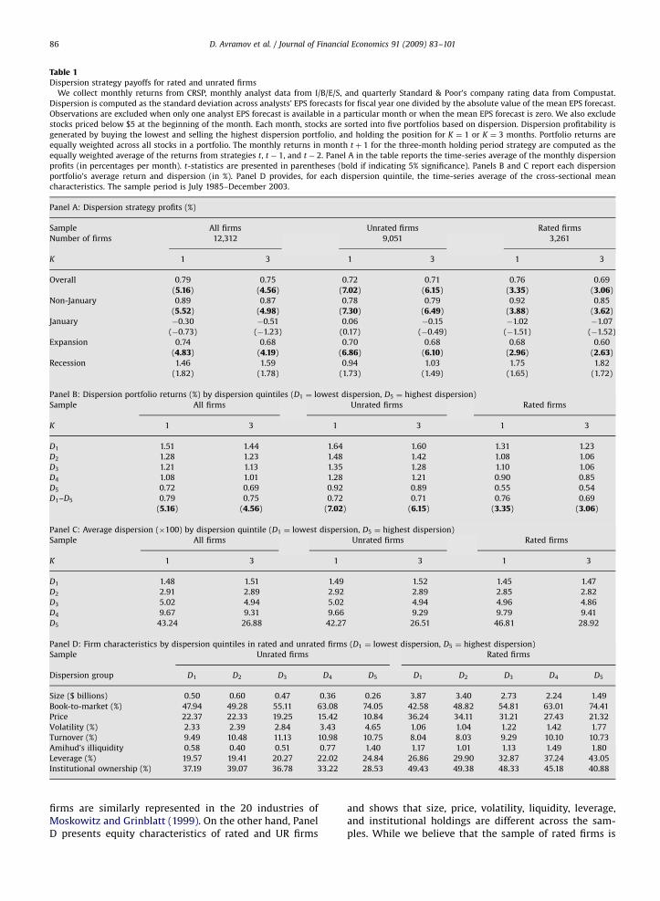
Dispersion profitability is presented in Panel A ofTable 1. Starting with the entire universe of stocks, wedemonstrate that buying low dispersion stocks, sellinghigh dispersion stocks, and holding the position for onemonth (three months) yields a statistically significantpayoff of 79 (75) basis points per month. The correspond-ing payoffs for the rated firms are 76 (69) basis points andfor the UR firms the payoffs are 72 (71) basis pointsper month. Note that the dispersion profitability existsonly in non-January months. Dispersion profitability is ingeneral negative, albeit insignificantly so, in January, andis statistically significant during expansions, but notduring recessions.

Panel B of Table 1 displays the returns of the fivedispersion portfolios with D1 (D5) denoting the portfoliowith the lowest (highest) dispersion in analysts’ earningsforecasts. Dispersion profitability is measured by thereturn differential between portfolios D1 and D5. Observethat for holding periods of both one month (K ¼ 1) andthree months (K ¼ 3), the dispersion portfolio returnsdecline monotonically as we move from portfolio D1 to D5.This pattern is consistent with previous work and holdsfor the entire universe of stocks, as well as for the ratedand UR firms. While there is a difference in the portfolioreturns for the rated and UR firms, the return differentialfor D1 � D5 is about the same.

Panel C of Table 1 presents the mean dispersionmeasures of the five dispersion portfolios for all firms aswell as for rated and UR firms. The evidence suggests thatmean dispersion measures for rated and UR firms arequite similar. To illustrate, for the lowest dispersionportfolio (D1) the mean dispersion measures over a one-and three-month holding period based on UR (rated) firmsare 1.49 and 1.52 (1.45 and 1.47), respectively. Similarly,for the highest dispersion portfolio (D5) the meandispersion measures for UR firms (rated firms) are 42.27and 26.51 (46.81 and 28.92), respectively.

Overall, the evidence in the three panels of Table 1suggests that while there are differences across rated andUR firms, the sample of rated firms is representativeenough in capturing the dispersion effect in the cross-section of returns. Of course, it is hard to be certain thatthe UR firms are not different from the rated firms alongsome other dimensions that could impact our results.Indeed, on one hand we confirm that both rated and UR

ARTICLE IN PRESS

Table 1Dispersion strategy payoffs for rated and unrated firms

We collect monthly returns from CRSP, monthly analyst data from I/B/E/S, and quarterly Standard & Poor’s company rating data from Compustat.

Dispersion is computed as the standard deviation across analysts’ EPS forecasts for fiscal year one divided by the absolute value of the mean EPS forecast.

Observations are excluded when only one analyst EPS forecast is available in a particular month or when the mean EPS forecast is zero. We also exclude

stocks priced below $5 at the beginning of the month. Each month, stocks are sorted into five portfolios based on dispersion. Dispersion profitability is

generated by buying the lowest and selling the highest dispersion portfolio, and holding the position for K ¼ 1 or K ¼ 3 months. Portfolio returns are

equally weighted across all stocks in a portfolio. The monthly returns in month t þ 1 for the three-month holding period strategy are computed as the

equally weighted average of the returns from strategies t, t � 1, and t � 2. Panel A in the table reports the time-series average of the monthly dispersion

profits (in percentages per month). t-statistics are presented in parentheses (bold if indicating 5% significance). Panels B and C report each dispersion

portfolio’s average return and dispersion (in %). Panel D provides, for each dispersion quintile, the time-series average of the cross-sectional mean

characteristics. The sample period is July 1985–December 2003.

Panel A: Dispersion strategy profits (%)

Sample All firms Unrated firms Rated firms

Number of firms 12,312 9,051 3,261

K 1 3 1 3 1 3

Overall 0.79 0.75 0.72 0.71 0.76 0.69

(5.16) (4.56) (7.02) (6.15) (3.35) (3.06)

Non-January 0.89 0.87 0.78 0.79 0.92 0.85

(5.52) (4.98) (7.30) (6.49) (3.88) (3.62)

January �0.30 �0.51 0.06 �0.15 �1.02 �1.07

(�0.73) (�1.23) (0.17) (�0.49) (�1.51) (�1.52)

Expansion 0.74 0.68 0.70 0.68 0.68 0.60

(4.83) (4.19) (6.86) (6.10) (2.96) (2.63)

Recession 1.46 1.59 0.94 1.03 1.75 1.82

(1.82) (1.78) (1.73) (1.49) (1.65) (1.72)

Panel B: Dispersion portfolio returns (%) by dispersion quintiles (D1 ¼ lowest dispersion, D5 ¼ highest dispersion)


K 1 3 1 3 1 3

D1 1.51 1.44 1.64 1.60 1.31 1.23

D2 1.28 1.23 1.48 1.42 1.08 1.06

D3 1.21 1.13 1.35 1.28 1.10 1.06

D4 1.08 1.01 1.28 1.21 0.90 0.85

D5 0.72 0.69 0.92 0.89 0.55 0.54

D1–D5 0.79 0.75 0.72 0.71 0.76 0.69

(5.16) (4.56) (7.02) (6.15) (3.35) (3.06)

Panel C: Average dispersion (�100) by dispersion quintile (D1 ¼ lowest dispersion, D5 ¼ highest dispersion)


K 1 3 1 3 1 3

D1 1.48 1.51 1.49 1.52 1.45 1.47

D2 2.91 2.89 2.92 2.89 2.85 2.82

D3 5.02 4.94 5.02 4.94 4.96 4.86

D4 9.67 9.31 9.66 9.29 9.79 9.41

D5 43.24 26.88 42.27 26.51 46.81 28.92

Panel D: Firm characteristics by dispersion quintiles in rated and unrated firms (D1 ¼ lowest dispersion, D5 ¼ highest dispersion)

Sample Unrated firms Rated firms

Dispersion group D1 D2 D3 D4 D5 D1 D2 D3 D4 D5

Size ($ billions) 0.50 0.60 0.47 0.36 0.26 3.87 3.40 2.73 2.24 1.49

Book-to-market (%) 47.94 49.28 55.11 63.08 74.05 42.58 48.82 54.81 63.01 74.41

Price 22.37 22.33 19.25 15.42 10.84 36.24 34.11 31.21 27.43 21.32

Volatility (%) 2.33 2.39 2.84 3.43 4.65 1.06 1.04 1.22 1.42 1.77

Turnover (%) 9.49 10.48 11.13 10.98 10.75 8.04 8.03 9.29 10.10 10.73

Amihud’s illiquidity 0.58 0.40 0.51 0.77 1.40 1.17 1.01 1.13 1.49 1.80

Leverage (%) 19.57 19.41 20.27 22.02 24.84 26.86 29.90 32.87 37.24 43.05

Institutional ownership (%) 37.19 39.07 36.78 33.22 28.53 49.43 49.38 48.33 45.18 40.88


firms are similarly represented in the 20 industries ofMoskowitz and Grinblatt (1999). On the other hand, PanelD presents equity characteristics of rated and UR firms

and shows that size, price, volatility, liquidity, leverage,and institutional holdings are different across the sam-ples. While we believe that the sample of rated firms is

ARTICLE IN PRESS

Table 2Composition of dispersion portfolios

Dispersion portfolios are constructed as explained in Table 1. The first

three columns show, for each dispersion portfolio, the percentage of

stocks that are unrated, rated investment grade, or rated non-investment

grade. The next four columns exhibit the equally weighted average

returns. The last column reports the average numerical S&P credit rating.

The numeric S&P rating is ascending in credit risk, i.e., AAA ¼ 1,

AAþ ¼ 2, AA ¼ 3, AA� ¼ 4, Aþ ¼ 5, A ¼ 6, A� ¼ 7, BBBþ ¼ 8, BBB ¼ 9,

BBB� ¼ 10, BBþ ¼ 11, BB ¼ 12, BB� ¼ 13, Bþ ¼ 14, B ¼ 15, B� ¼ 16,

CCCþ ¼ 17, CCC ¼ 18, CCC� ¼ 19, CC ¼ 20, C ¼ 21, D ¼ 22. The sample

consists of 12,312 companies over the period of July 1985–December

2003. The t-statistics are presented in parentheses, bold indicating 5%

significance.

Notation: UR ¼‘‘unrated’’; IG ¼‘‘investment grade’’, S&P rating BBB�

or better; NIG ¼‘‘non-investment grade’’, S&P rating BBþ or worse.

D1–D5 are dispersion quintiles where D1 ¼ lowest dispersion,

D5 ¼ highest dispersion.


representative along many important dimensions, oneshould bear in mind the data limitations of our analysis.

Finally, we measure the cross-sectional correlationbetween dispersion and numerical credit rating for eachmonth in the sample. The Spearman rank cross-sectionalcorrelation averages 0.39, suggesting that dispersion andcredit rating could proxy for the same underlyingeconomic fundamental. We argue that this economicfundamental is financial distress. At the same time, creditrating is not merely a statistical proxy for dispersion, aswe will show below. It is a different economic measurethat captures both the dispersion effect in the cross-section of returns as well as the impact of size, turnover,leverage, and other firm-level characteristics on therelation between dispersion and returns.

Percentage of stocks Returns (% per month) Rating

Portfolio UR IG NIG UR IG NIG All

D1 65.12 27.42 7.46 1.64 1.32 1.20 1.51 7.20

D2 59.10 32.79 8.10 1.48 1.23 0.45 1.28 7.43

D3 60.18 29.71 10.11 1.35 1.25 0.71 1.21 8.14

D4 60.82 25.50 13.68 1.28 1.19 0.47 1.08 9.05

D5 59.04 17.96 23.00 0.92 1.01 0.19 0.72 10.88

D1–D5 0.72 0.31 1.01 0.79

(7.02) (1.41) (3.64) (5.16)

3 We have also experimented (results are available upon request)

with 5� 3, 3� 5, as well as 3� 3 credit rating-dispersion portfolios and

have confirmed that the empirical evidence is unchanged.4 We have checked that the sequential sorting procedure is not

driving the results. The payoffs with independent sorts are similar.5 Results are similar if the risk-adjustment is based on the CAPM or

the Fama and French (1993) factors.

3. Results

3.1. Credit rating and dispersion in analysts’ earnings

forecasts

To establish the first link between credit risk and theprofitability of trading strategies based on dispersion inearnings forecasts, we examine the credit rating profile ofthe five dispersion portfolios. The results are exhibited inTable 2. The lowest dispersion portfolio (D1) is heavilytilted towards the best quality firms. The average creditrating for this portfolio is 7.20, corresponding to anA� rating. On the other hand, the dispersion portfolio D5

is populated with the highest credit risk stocks and has anaverage credit rating of 10.88, corresponding to a BBþrating, which is a below IG rating. In general, higherdispersion portfolios contain lower quality stocks as thenumerical value of credit rating increases monotonicallywith dispersion.

Table 2 also displays the proportion of UR, IG, and NIGfirms within each of the five dispersion portfolios. IGcorresponds to an S&P rating of BBB� or better. Note thatrated firms populate all examined portfolios with frac-tions ranging between 34.88% and 40.96%. Moreover,portfolios D1, D2, D3, and D4 consist mostly of higherquality firms. The highest dispersion portfolio, D5, is theonly one tilted towards NIG stocks.

Observe from Table 2 that dispersion profitability is afacet of NIG firms and is virtually non-existent otherwise.In particular, implementing dispersion trading strategiesof buying low dispersion stocks and selling high disper-sion stocks (D1 � D5), yields a statistically insignificantpayoff of 31 basis points per month among IG firms. Incontrast, implementing dispersion strategies among NIGfirms yields a highly significant payoff of 101 basis pointsper month.

In addition, note that for each dispersion group, highercredit quality firms realize higher returns than lowerquality firms. For the lowest dispersion portfolio, IG stocksyield a monthly payoff of 1.32% per month, whereas thecorresponding return for NIG stocks is 1.20%. Indeed, asnoted earlier, prior research shows that higher default riskstocks earn, on average, lower returns. Our sample of ratedfirms clearly captures this apparent anomalous pattern.

To get a better sense of the source of dispersionprofitability, we consider 25 credit risk-dispersion portfo-lios. In particular, we form portfolios as the intersection offive credit rating and five dispersion groups.3 Credit risk-dispersion groups are formed sequentially, first sorting oncredit rating and then on dispersion.4 The five credit riskgroups, C1–C5, are formed each month by sorting thesample of firms in that month into quintiles based on theircredit ratings. Each of the resulting credit rating groups isthen divided into five dispersion portfolios, D1–D5.

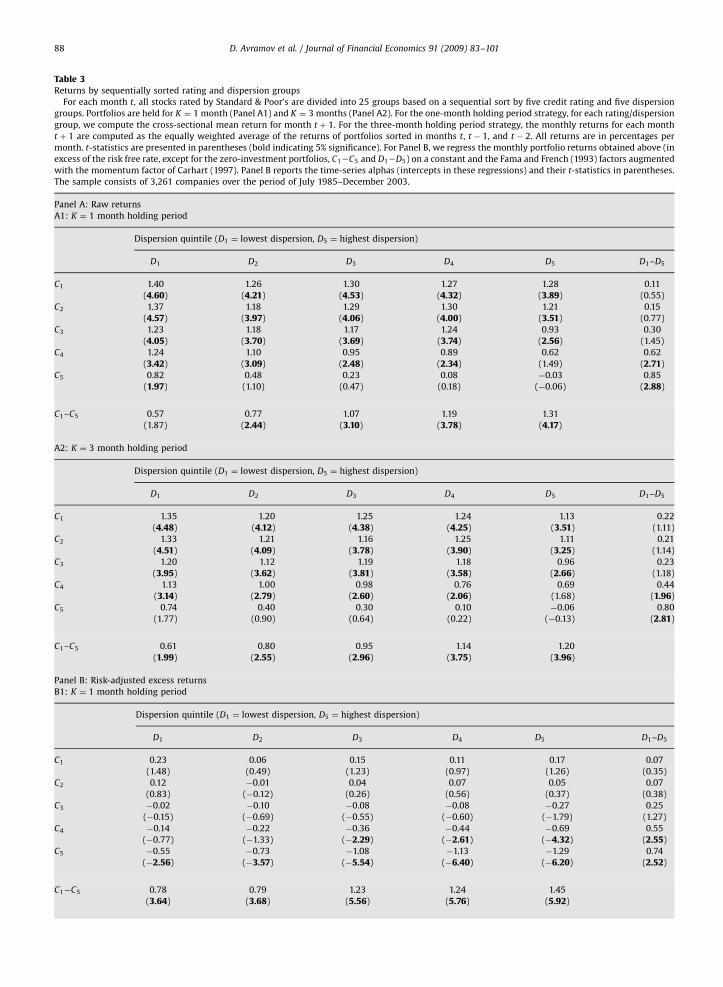
Table 3 presents average monthly raw and risk-adjusted returns for the 25 credit risk-dispersion portfo-lios, as well as the dispersion profitability (D1 � D5) acrosscredit rating quintiles, and the credit rating profitability(C1 � C5) across the dispersion quintiles. Monthly payoffsare presented for holding periods of one month (Panels A1and B1) as well as three months (Panels A2 and B2). PanelsA1 and A2 present raw returns and Panels B1 and B2present risk-adjusted excess returns (or time-seriesalphas) based on the Fama and French (1993) factorsaugmented by the momentum factor of Carhart (1997).5

We observe that dispersion profitability stronglydepends upon credit rating. Focusing on the one-monthinvestment horizon (findings for the three-month horizonare similar), for the C1, C2, and C3 credit rating quintiles,

ARTICLE IN PRESS

Table 3Returns by sequentially sorted rating and dispersion groups

For each month t, all stocks rated by Standard & Poor’s are divided into 25 groups based on a sequential sort by five credit rating and five dispersion

groups. Portfolios are held for K ¼ 1 month (Panel A1) and K ¼ 3 months (Panel A2). For the one-month holding period strategy, for each rating/dispersion

group, we compute the cross-sectional mean return for month t þ 1. For the three-month holding period strategy, the monthly returns for each month

t þ 1 are computed as the equally weighted average of the returns of portfolios sorted in months t, t � 1, and t � 2. All returns are in percentages per

month. t-statistics are presented in parentheses (bold indicating 5% significance). For Panel B, we regress the monthly portfolio returns obtained above (in

excess of the risk free rate, except for the zero-investment portfolios, C12C5 and D12D5) on a constant and the Fama and French (1993) factors augmented

with the momentum factor of Carhart (1997). Panel B reports the time-series alphas (intercepts in these regressions) and their t-statistics in parentheses.

The sample consists of 3,261 companies over the period of July 1985–December 2003.

Panel A: Raw returns

A1: K ¼ 1 month holding period

Dispersion quintile (D1 ¼ lowest dispersion, D5 ¼ highest dispersion)

D1 D2 D3 D4 D5 D1–D5

C1 1.40 1.26 1.30 1.27 1.28 0.11

(4.60) (4.21) (4.53) (4.32) (3.89) (0.55)

C2 1.37 1.18 1.29 1.30 1.21 0.15

(4.57) (3.97) (4.06) (4.00) (3.51) (0.77)

C3 1.23 1.18 1.17 1.24 0.93 0.30

(4.05) (3.70) (3.69) (3.74) (2.56) (1.45)

C4 1.24 1.10 0.95 0.89 0.62 0.62

(3.42) (3.09) (2.48) (2.34) (1.49) (2.71)

C5 0.82 0.48 0.23 0.08 �0.03 0.85

(1.97) (1.10) (0.47) (0.18) (�0.06) (2.88)

C1–C5 0.57 0.77 1.07 1.19 1.31

(1.87) (2.44) (3.10) (3.78) (4.17)

A2: K ¼ 3 month holding period


D1 D2 D3 D4 D5 D1–D5

C1 1.35 1.20 1.25 1.24 1.13 0.22

(4.48) (4.12) (4.38) (4.25) (3.51) (1.11)

C2 1.33 1.21 1.16 1.25 1.11 0.21

(4.51) (4.09) (3.78) (3.90) (3.25) (1.14)

C3 1.20 1.12 1.19 1.18 0.96 0.23

(3.95) (3.62) (3.81) (3.58) (2.66) (1.18)

C4 1.13 1.00 0.98 0.76 0.69 0.44

(3.14) (2.79) (2.60) (2.06) (1.68) (1.96)

C5 0.74 0.40 0.30 0.10 �0.06 0.80

(1.77) (0.90) (0.64) (0.22) (�0.13) (2.81)

C1–C5 0.61 0.80 0.95 1.14 1.20

(1.99) (2.55) (2.96) (3.75) (3.96)

Panel B: Risk-adjusted excess returns

B1: K ¼ 1 month holding period


D1 D2 D3 D4 D5 D1–D5

C1 0.23 0.06 0.15 0.11 0.17 0.07

(1.48) (0.49) (1.23) (0.97) (1.26) (0.35)

C2 0.12 �0.01 0.04 0.07 0.05 0.07

(0.83) (�0.12) (0.26) (0.56) (0.37) (0.38)

C3 �0.02 �0.10 �0.08 �0.08 �0.27 0.25

(�0.15) (�0.69) (�0.55) (�0.60) (�1.79) (1.27)

C4 �0.14 �0.22 �0.36 �0.44 �0.69 0.55

(�0.77) (�1.33) (�2.29) (�2.61) (�4.32) (2.55)

C5 �0.55 �0.73 �1.08 �1.13 �1.29 0.74

(�2.56) (�3.57) (�5.54) (�6.40) (�6.20) (2.52)

C1�C5 0.78 0.79 1.23 1.24 1.45

(3.64) (3.68) (5.56) (5.76) (5.92)


ARTICLE IN PRESS

B2: K ¼ 3 month holding period


D1 D2 D3 D4 D5 D1–D5

C1 0.22 0.07 0.14 0.11 0.06 0.15

(1.45) (0.58) (1.18) (1.07) (0.54) (0.90)

C2 0.14 0.03 �0.01 0.06 �0.04 0.18

(1.00) (0.22) (�0.10) (0.48) (�0.34) (1.06)

C3 �0.03 �0.10 0.01 �0.12 �0.24 0.21

(�0.21) (�0.87) (0.05) (�0.97) (�1.62) (1.11)

C4 �0.18 �0.28 �0.28 �0.53 �0.59 0.41

(�0.99) (�1.91) (�1.98) (�3.85) (�3.77) (1.94)

C5 �0.59 �0.78 �0.98 �1.07 �1.27 0.68

(�2.86) (�4.14) (�5.63) (�6.67) (�6.25) (2.42)

C1–C5 0.80 0.85 1.12 1.19 1.33

(4.10) (4.33) (5.89) (6.11) (5.84)

Table 3 (continued)


dispersion profitability, D12D5, is 11, 15, and 30 basispoints per month, respectively, and is insignificant atconventional levels. The payoff is statistically and eco-nomically significant at 0.62% per month for the fourthquintile and 0.85% per month for the highest credit riskquintile. Note that the dispersion profitability increasesmonotonically with credit risk. Profitability across creditrisk quintiles, C12C5, also increases monotonically withdispersion from 0.57% for the lowest dispersion quintile to1.31% per month for the highest dispersion quintile. TheC12C5 payoffs are significant in all dispersion groups.

Panels B1 and B2 of Table 3 present alphas from time-series regressions of the 25 credit rating-dispersion sortedportfolio excess returns and of the zero-cost portfolioreturns (D12D5 and C12C5) on the Fama and French(1993) factors augmented by the momentum factor ofCarhart (1997). Alphas of the D12D5 portfolios increasewith credit risk and are statistically and economicallysignificant only for the two highest credit risk quintilesgiven by 55 ðC4Þ and 74 ðC5Þ basis points per month.Profitability across credit risk quintiles, C12C5, continuesto increases monotonically with dispersion from 0.78%(80%) for the lowest dispersion quintile to 1.45% (1.33%)per month for the highest dispersion quintile in the one-month (three-months) holding strategy. These payoffs areall significant at the 5% level in all dispersion groups.

Indeed, one could argue that just as much as creditconditions could capture the dispersion effect, the disper-sion effect could also capture the credit risk effect. There isa clear interaction between dispersion and credit risk butit is unclear, at this stage, which measure, if any, governsthis interaction. Below, we show that the impact of creditrisk is more prominent possibly because credit ratings area better proxy for financial distress than analysts’ earningsforecast dispersion.

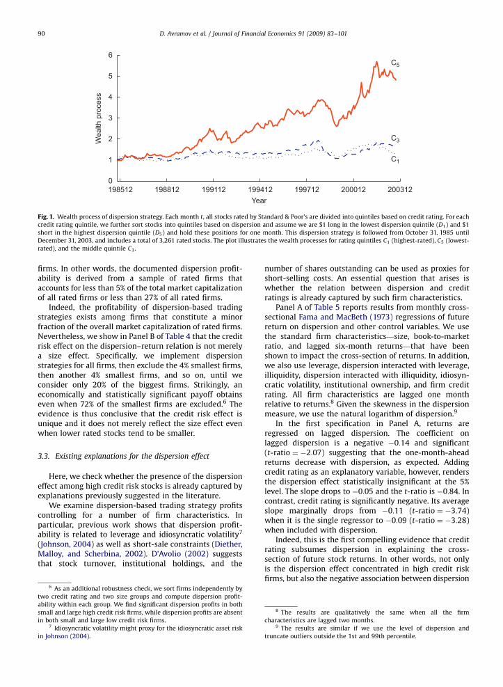
Table 3 presents the means and the statisticalsignificance of dispersion-based trading strategies. To getsome perspective about the dynamics of dispersionprofitability, we plot in Fig. 1 the wealth accumulated bytaking long (short) positions in stocks with low (high)dispersion in analysts’ forecasts starting from October

1985. Investing $1 in dispersion strategies implementedamong the highest quality stocks (C1) realizes a payoff of$1.28 in December 2003. The corresponding payoff ismuch larger at $4.82 when the investment universe iscomprised of the lowest quality stocks (C5). Moreover, it isevident that the payoff differential between C1 and C5

firms is quite steady throughout the entire sample as itdoes not concentrate in one particular period.

3.2. Dispersion profitability among subsamples of rated

firms

The analysis thus far has examined the relationbetween dispersion profitability and credit risk usingportfolio strategies based on double sorting, first by creditquality and then by dispersion. We now attempt to trackmore closely the subsample of firms that drives thesignificant dispersion payoffs. We implement the tradi-tional dispersion strategies based only on dispersion inearnings forecasts, but for different investment subsam-ples. In particular, we start with the entire sample of ratedfirms and then sequentially exclude firms with the highestcredit risk.

The dispersion profitability is reported in Table 4. Alsoprovided is the percentage of market capitalizationrepresented by each rating subsample, as well as thepercentage of the total number of firms included in eachsubsample. These two measures are computed eachmonth, and we report the time-series average. In PanelA of Table 4 the dispersion portfolio cutoffs are recom-puted for each rating subsample to maintain a (roughly)equal number of firms across the five dispersion portfo-lios. We have also implemented the same analysis usingfixed cutoffs based upon the entire universe of rated firms.Results (available upon request) are virtually identical.

It is apparent that the dispersion strategy payoff isinsignificant at the 5% level for subsamples that containstocks in the rating range AAA–BBþ. Strikingly, thissubsample accounts for 95.58% of the market capitaliza-tion of rated firms and 73.86% of the total number of rated

ARTICLE IN PRESS

198512 198812 199112 199412 199712 200012 200312

0

1

2

3

4

5

6

Wealth p

rocess

Year

C1

C3

C5

Fig. 1. Wealth process of dispersion strategy. Each month t, all stocks rated by Standard & Poor’s are divided into quintiles based on credit rating. For each

credit rating quintile, we further sort stocks into quintiles based on dispersion and assume we are $1 long in the lowest dispersion quintile (D1) and $1

short in the highest dispersion quintile (D5) and hold these positions for one month. This dispersion strategy is followed from October 31, 1985 until

December 31, 2003, and includes a total of 3,261 rated stocks. The plot illustrates the wealth processes for rating quintiles C1 (highest-rated), C5 (lowest-

rated), and the middle quintile C3.


firms. In other words, the documented dispersion profit-ability is derived from a sample of rated firms thataccounts for less than 5% of the total market capitalizationof all rated firms or less than 27% of all rated firms.

Indeed, the profitability of dispersion-based tradingstrategies exists among firms that constitute a minorfraction of the overall market capitalization of rated firms.Nevertheless, we show in Panel B of Table 4 that the creditrisk effect on the dispersion–return relation is not merelya size effect. Specifically, we implement dispersionstrategies for all firms, then exclude the 4% smallest firms,then another 4% smallest firms, and so on, until weconsider only 20% of the biggest firms. Strikingly, aneconomically and statistically significant payoff obtainseven when 72% of the smallest firms are excluded.6 Theevidence is thus conclusive that the credit risk effect isunique and it does not merely reflect the size effect evenwhen lower rated stocks tend to be smaller.

3.3. Existing explanations for the dispersion effect

Here, we check whether the presence of the dispersioneffect among high credit risk stocks is already captured byexplanations previously suggested in the literature.

We examine dispersion-based trading strategy profitscontrolling for a number of firm characteristics. Inparticular, previous work shows that dispersion profit-ability is related to leverage and idiosyncratic volatility7

(Johnson, 2004) as well as short-sale constraints (Diether,Malloy, and Scherbina, 2002). D’Avolio (2002) suggeststhat stock turnover, institutional holdings, and the

6 As an additional robustness check, we sort firms independently by

two credit rating and two size groups and compute dispersion profit-

ability within each group. We find significant dispersion profits in both

small and large high credit risk firms, while dispersion profits are absent

in both small and large low credit risk firms.7 Idiosyncratic volatility might proxy for the idiosyncratic asset risk

in Johnson (2004).

number of shares outstanding can be used as proxies forshort-selling costs. An essential question that arises iswhether the relation between dispersion and creditratings is already captured by such firm characteristics.

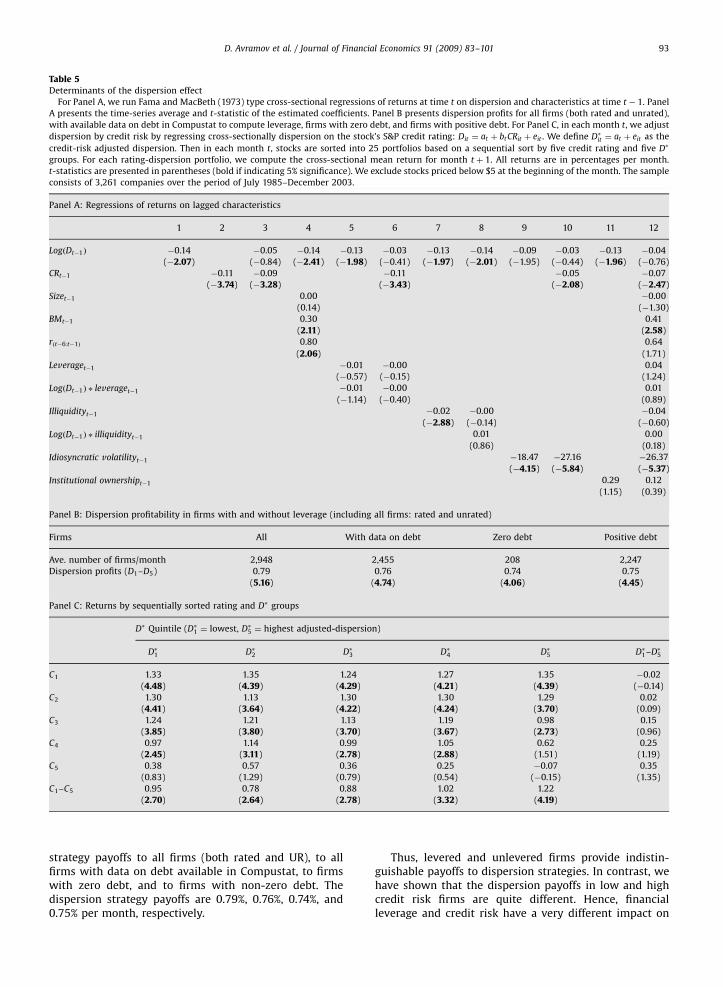
Panel A of Table 5 reports results from monthly cross-sectional Fama and MacBeth (1973) regressions of futurereturn on dispersion and other control variables. We usethe standard firm characteristics—size, book-to-marketratio, and lagged six-month returns—that have beenshown to impact the cross-section of returns. In addition,we also use leverage, dispersion interacted with leverage,illiquidity, dispersion interacted with illiquidity, idiosyn-cratic volatility, institutional ownership, and firm creditrating. All firm characteristics are lagged one monthrelative to returns.8 Given the skewness in the dispersionmeasure, we use the natural logarithm of dispersion.9

In the first specification in Panel A, returns areregressed on lagged dispersion. The coefficient onlagged dispersion is a negative �0:14 and significant(t-ratio ¼ �2:07) suggesting that the one-month-aheadreturns decrease with dispersion, as expected. Addingcredit rating as an explanatory variable, however, rendersthe dispersion effect statistically insignificant at the 5%level. The slope drops to �0:05 and the t-ratio is �0:84. Incontrast, credit rating is significantly negative. Its averageslope marginally drops from �0:11 (t-ratio ¼ �3:74)when it is the single regressor to �0:09 (t-ratio ¼ �3:28)when included with dispersion.

Indeed, this is the first compelling evidence that creditrating subsumes dispersion in explaining the cross-section of future stock returns. In other words, not onlyis the dispersion effect concentrated in high credit riskfirms, but also the negative association between dispersion

8 The results are qualitatively the same when all the firm

characteristics are lagged two months.9 The results are similar if we use the level of dispersion and

truncate outliers outside the 1st and 99th percentile.

ARTICLE IN PRESS

Table 4Dispersion strategy payoffs over diminishing subsamples

Dispersion portfolios are constructed as explained in Table 1. Each subsequent row in Panel A (Panel B) represents a monotonically decreasing sample of

stocks obtained by sequentially excluding firms with the worst credit rating (smallest market capitalization). The first column characterizes each

subsample. The second column presents the raw monthly profits from the dispersion strategy for each subsample of firms (t-statistics are in parentheses,

bold if indicating 5% significance). The third column shows the market capitalization of the given subsample as a percentage of the overall market

capitalization of S&P rated firms. The fourth (fifth) column provides the average number (percentage) of firms per month in each subsample. The sample

contains 3,261 companies over the period of July 1985–December 2003.

Panel A: Dispersion profits by sequentially removing worst-rated stocks

Stock sample Dispersion profits Percent of total market cap Number of firms Percentage of firms

All firms 0.76 100.00 1,154.00 100.00

(3.35)

AAA�C 0.75 99.99 1,153.52 99.96

(3.33)

AAA�CC 0.75 99.99 1,153.52 99.96

(3.33)

AAA�CCC� 0.76 99.98 1,153.19 99.93

(3.35)

AAA�CCC 0.76 99.98 1,152.91 99.91

(3.34)

AAA�CCCþ 0.73 99.97 1,151.61 99.79

(3.25)

AAA�B� 0.71 99.93 1,148.21 99.50

(3.18)

AAA�B 0.68 99.70 1,135.56 98.40

(3.07)

AAA�Bþ 0.61 99.20 1,109.11 96.11

(2.81)

AAA�BB� 0.53 98.30 1,023.83 88.72

(2.57)

AAA�BB 0.40 97.05 931.90 80.75

(1.98)

AAA�BBþ 0.32 95.58 852.36 73.86

(1.58)

AAA�BBB� 0.26 93.73 784.52 67.98

(1.35)

AAA�BBB 0.22 90.07 687.38 59.56

(1.13)

AAA�BBBþ 0.18 84.03 560.71 48.59

(0.92)

Panel B: Dispersion profits by sequentially removing smallest stocks


All firms 0.76 100.00 1,154.00 100.00

(3.35)

Biggest 96% 0.67 99.96 1,107.84 96.00

(2.91)

Biggest 92% 0.66 99.86 1,061.70 92.00

(2.86)

Biggest 88% 0.67 99.71 1,015.57 88.00

(2.86)

Biggest 84% 0.60 99.51 969.35 84.00

(2.56)

Biggest 80% 0.61 99.27 923.21 80.00

(2.56)

Biggest 76% 0.54 98.97 877.07 76.00

(2.26)

Biggest 72% 0.53 98.61 830.86 72.00

(2.23)

Biggest 68% 0.51 98.17 784.75 68.00

(2.11)

Biggest 64% 0.51 97.65 738.60 64.00

(2.11)

Biggest 60% 0.49 97.05 692.42 60.00

(1.96)

Biggest 56% 0.48 96.34 646.24 56.00

(1.93)

Biggest 52% 0.46 95.52 600.08 52.00

(1.84)


ARTICLE IN PRESS

Table 4 (continued )

Panel B: Dispersion profits by sequentially removing smallest stocks


Biggest 48% 0.51 94.54 553.97 48.00

(1.99)

Biggest 44% 0.51 93.40 507.81 44.00

(1.98)

Biggest 40% 0.48 92.06 461.63 40.00

(1.84)

Biggest 36% 0.44 90.48 415.46 36.00

(1.66)

Biggest 32% 0.44 88.58 369.30 32.00

(1.66)

Biggest 28% 0.55 86.27 323.19 28.01

(2.01)

Biggest 24% 0.50 83.47 276.98 24.00

(1.81)

Biggest 20% 0.48 79.96 230.85 20.00

(1.64)


and future returns is non-existent when credit rating isused as a control variable. In contrast, including thestandard firm characteristics of size, book-to-market ratio,and lagged six-month returns does not render the impactof dispersion on returns insignificant.

Next, as suggested by Johnson (2004), we include firmleverage and the interaction of leverage and dispersion.Leverage is measured as the most recent book value ofdebt divided by the sum of the book value of debt and themarket value of equity. The evidence shows that neither ofthese measures has an impact on the significance of thedispersion coefficient but the credit rating does. Indeed,this apparently contradicts the relevance of leverage inJohnson (2004) and could be due to the different samplesused, as we focus on firms rated by S&P. However, Sadkaand Scherbina (2007) also find a negative but statisticallyinsignificant coefficient on leverage and leverage inter-acted with dispersion in their sample of all NYSE-listedfirms with December fiscal year end.

We also examine the impact of Amihud’s (2002)illiquidity measure, idiosyncratic volatility, and institu-tional ownership on the dispersion–return relation. Whilethe coefficient on illiquidity is significantly negative, itdoes not explain away the significance of dispersion.10 Thecoefficient of idiosyncratic volatility is also significantlynegative but it does not capture the dispersion–returnrelation. Finally, institutional ownership is not significantand does not call into question the dispersion effect in oursample. Indeed, the relation between analyst forecastdispersion and future returns among rated firms is robustto the inclusion of all variables except for credit ratings.

10 We bear in mind that our results may be different from Sadka and

Scherbina (2007) because they include all NYSE firms with December

fiscal year end and a different measure of illiquidity—a dummy for the

top 20% of price impact (PI)—in their cross-sectional regressions to

explain the persistence of the dispersion effect through time.

More importantly, variables that proxy for short-selling costs such as illiquidity, institutional holdings,and firm size are all statistically insignificant and do notimpact the relation between dispersion and returns.11 Thisis important because Diether, Malloy, and Scherbina(2002) argue that short-sale constraints play an importantrole in generating the dispersion–return relation. The ideais that in stocks with high dispersion (which proxies fordifferences in agent beliefs) optimistic investors bid pricesup and short-sale constraints prevent pessimistic viewsfrom being reflected into the stock price, thus, causing thehigh dispersion stocks to become temporarily overpriced.The dispersion effect emerges as this overpricing iscorrected over time. However, the results show that thestandard proxies for short-sale costs are insufficient inexplaining the dispersion effect.

Moreover, our results suggest that, while illiquidity canexplain the persistence of the dispersion effect, as shownby Sadka and Scherbina (2007), illiquidity does notexplain why the dispersion effect exists in the first place.While low-rated stocks are in general illiquid, it is thecredit rating and not illiquidity that drives the impact offorecast dispersion on returns.

As noted earlier, Johnson (2004) argues that analystforecast dispersion is a proxy for unpriced informationrisk and, for levered firms, expected returns shoulddecrease with idiosyncratic asset risk. Thus, the dispersioneffect obtains even when there is no cross-sectionalrelation between dispersion of beliefs and fundamentalrisk. One prediction of the Johnson (2004) model is thatthe dispersion effect should be stronger as firm leverageincreases. In Panel B of Table 5 we examine the dispersion

11 We also used turnover instead of illiquidity in the regressions and

the results were similar. Moreover, we have considered all interactions

among the short-sale constraint variables to account for non-linear

short-sale effects. The dispersion effect remains significant in their

presence.

ARTICLE IN PRESS

Table 5Determinants of the dispersion effect

For Panel A, we run Fama and MacBeth (1973) type cross-sectional regressions of returns at time t on dispersion and characteristics at time t � 1. Panel

A presents the time-series average and t-statistic of the estimated coefficients. Panel B presents dispersion profits for all firms (both rated and unrated),

with available data on debt in Compustat to compute leverage, firms with zero debt, and firms with positive debt. For Panel C, in each month t, we adjust

dispersion by credit risk by regressing cross-sectionally dispersion on the stock’s S&P credit rating: Dit ¼ at þ btCRit þ eit . We define D�it ¼ at þ eit as the

credit-risk adjusted dispersion. Then in each month t, stocks are sorted into 25 portfolios based on a sequential sort by five credit rating and five D�

groups. For each rating-dispersion portfolio, we compute the cross-sectional mean return for month t þ 1. All returns are in percentages per month.

t-statistics are presented in parentheses (bold if indicating 5% significance). We exclude stocks priced below $5 at the beginning of the month. The sample

consists of 3,261 companies over the period of July 1985–December 2003.

Panel A: Regressions of returns on lagged characteristics

1 2 3 4 5 6 7 8 9 10 11 12

LogðDt�1Þ �0.14 �0.05 �0.14 �0.13 �0.03 �0.13 �0.14 �0.09 �0.03 �0.13 �0.04

(�2.07) (�0.84) (�2.41) (�1.98) (�0.41) (�1.97) (�2.01) (�1.95) (�0.44) (�1.96) (�0.76)

CRt�1 �0.11 �0.09 �0.11 �0.05 �0.07

(�3.74) (�3.28) (�3.43) (�2.08) (�2.47)

Sizet�1 0.00 �0.00

(0.14) (�1.30)

BMt�1 0.30 0.41

(2.11) (2.58)

rðt�6:t�1Þ 0.80 0.64

(2.06) (1.71)

Leveraget�1 �0.01 �0.00 0.04

(�0.57) (�0.15) (1.24)

LogðDt�1Þ � leveraget�1 �0.01 �0.00 0.01

(�1.14) (�0.40) (0.89)

Illiquidityt�1 �0.02 �0.00 �0.04

(�2.88) (�0.14) (�0.60)

LogðDt�1Þ � illiquidityt�1 0.01 0.00

(0.86) (0.18)

Idiosyncratic volatilityt�1 �18.47 �27.16 �26.37

(�4.15) (�5.84) (�5.37)

Institutional ownershipt�1 0.29 0.12

(1.15) (0.39)

Panel B: Dispersion profitability in firms with and without leverage (including all firms: rated and unrated)

Firms All With data on debt Zero debt Positive debt

Ave. number of firms/month 2,948 2,455 208 2,247

Dispersion profits (D1–D5) 0.79 0.76 0.74 0.75

(5.16) (4.74) (4.06) (4.45)

Panel C: Returns by sequentially sorted rating and D� groups

D� Quintile (D�1 ¼ lowest, D�5 ¼ highest adjusted-dispersion)

D�1 D�2 D�3 D�4 D�5 D�1–D�5

C1 1.33 1.35 1.24 1.27 1.35 �0.02

(4.48) (4.39) (4.29) (4.21) (4.39) (�0.14)

C2 1.30 1.13 1.30 1.30 1.29 0.02

(4.41) (3.64) (4.22) (4.24) (3.70) (0.09)

C3 1.24 1.21 1.13 1.19 0.98 0.15

(3.85) (3.80) (3.70) (3.67) (2.73) (0.96)

C4 0.97 1.14 0.99 1.05 0.62 0.25

(2.45) (3.11) (2.78) (2.88) (1.51) (1.19)

C5 0.38 0.57 0.36 0.25 �0.07 0.35

(0.83) (1.29) (0.79) (0.54) (�0.15) (1.35)

C1–C5 0.95 0.78 0.88 1.02 1.22

(2.70) (2.64) (2.78) (3.32) (4.19)


strategy payoffs to all firms (both rated and UR), to allfirms with data on debt available in Compustat, to firmswith zero debt, and to firms with non-zero debt. Thedispersion strategy payoffs are 0.79%, 0.76%, 0.74%, and0.75% per month, respectively.

Thus, levered and unlevered firms provide indistin-guishable payoffs to dispersion strategies. In contrast, wehave shown that the dispersion payoffs in low and highcredit risk firms are quite different. Hence, financialleverage and credit risk have a very different impact on

ARTICLE IN PRESS

12 We have also ensured that the results for other characteristics

such as idiosyncratic volatility and leverage are similar to those

presented.


the dispersion–return relation. Indeed, while creditrating is affected by financial leverage, we find that thetime-series average cross-sectional correlation betweencredit rating and financial leverage is 0.19 and rangesbetween �0:01 and 0.38 over the sample months. Indeed,a bad credit rating may be the result of high operatingleverage, high uncertainty about future profitabilityand growth, and/or volatility, even when financialleverage is low. Hence, our finding that financial leveragehas little impact on dispersion profitability motivates oursearch for an alternative explanation for the dispersioneffect.

Panel A of Table 5 shows that the dispersion–returnrelation becomes insignificant when controlling for creditrating. The multiple cross-sectional regression of futurereturns on the explanatory variables dispersion and creditrating is equivalent to the univariate regression of futurereturns on a credit rating-adjusted dispersion measure,where the adjusted-dispersion measure is computed asthe sum of intercept and residual from the cross-sectionalregression of dispersion on credit rating. By construction,the cross-sectional correlation between the rating-adjusted dispersion measure and credit rating is zero.Thus, to map the statistical evidence into an economicone, we construct monthly credit rating-adjusted disper-sion measures as monthly residuals in cross-sectionalregressions of dispersion on credit rating (of course, theintercept is constant across stocks for any given month).We then compute average payoffs for 25 portfoliosconstructed as the intersection of five credit rating groupsand five adjusted-dispersion groups, sorted first on creditrating. Panel C of Table 5 reports these average returns aswell as payoffs to implementing trading strategies basedon the adjusted-dispersion measure. We denote theportfolio with the lowest (highest) adjusted-dispersionmeasure by D�1 (D�5).

The evidence indicates that implementing investmentstrategies based on credit rating-adjusted dispersiongenerates payoffs that are not statistically significant oreconomically large for any of the credit rating groups.Specifically, the payoff differential between low and highadjusted-dispersion portfolios (D�1 � D�5) across the creditrating quintiles ranges from �2 basis points to 35 basispoints per month, all of which are insignificant. In otherwords, excluding the credit rating information fromdispersion yields an adjusted measure that has no powerto generate profitable trading strategies.

Panel A of Table 6 presents supporting evidence thatcredit risk is more prominent than existing explanationsfor the dispersion effect. Whereas in Panel C of Table 5dispersion was adjusted by credit rating, here we adjustreturns by credit rating. Credit rating-adjusted returns areobtained by subtracting from each stock return thecorresponding return of the credit rating decile to whichthe stock belongs. The traditional dispersion measureproduces insignificant dispersion profits among all creditrisk groups once the credit risk effect is removed fromstock returns. Focusing on Panel A, the credit risk-adjustedpayoffs to the dispersion strategy for the credit ratingquintiles are all less than 27 basis points per month, all ofwhich are insignificant. The significance of the dispersion

effect also disappears in the overall sample of rated firms(last line).

For robustness, in Panels B–E we compute dispersionprofits based on returns adjusted for equity characteris-tics suggested by alternative explanations for thedispersion effect. In particular, returns are adjusted forthe following characteristics: market capitalization,turnover, institutional ownership, and number ofshares outstanding.12 As before, characteristic-adjustedreturns are computed by subtracting from each stockreturn the corresponding return of the characteristicdecile to which the stock belongs. The dispersion strategypayoffs are still significant for the low-rated stocks(and for all rated stocks) even after adjusting for theabove characteristics. Thus, the dispersion strategy pay-offs are insignificant only when adjusting for credit ratings(Panel A).

Finally, we check that the credit risk effect on thedispersion–return relation is not captured by potentialindustry effects in the cross-section of returns. That is, weimplement dispersion strategies based on industry-adjusted returns following the industry groups examinedby Moskowitz and Grinblatt (1999). Our findings(available upon request) show that dispersion profitabilityis statistically and economically significant only for theworst credit quality firms.

In sum, the ability of dispersion to predict futurereturns is attributable to the predictive power of creditratings. The dispersion–return relation is significantlyweaker when either the dispersion measure or return isadjusted by credit risk. Since credit risk is negativelyassociated with the cross-section of future stock returns, itis not surprising that dispersion has also been negativelyrelated to future returns.

3.4. The dispersion–return relation during periods of

worsening credit conditions

Thus far we have shown that the credit rating levelhas a large impact on the dispersion effect. Next, weshow that it is indeed financial distress that is animportant driver of the dispersion effect. We examinefinancial distress in the context of credit rating down-grades. Our focus on downgrades follows previous workthat demonstrates an asymmetric response of futurereturns to credit rating changes. In particular, both Hand,Holthausen, and Leftwich (1992) and Dichev and Piotroski(2001) find considerable abnormal price declines follow-ing rating downgrades but no price advances followingupgrades.

In our context, rating downgrades possibly triggerhigher uncertainty about firm fundamentals as well asworsening fundamentals (potentially enhanced by sup-pliers, customers, and creditors abandoning the firm). Forfinancial distress to be the source of the dispersion effect,we have to show that analyst forecast dispersion increases

ARTICLE IN PRESS


around downgrades and that the dispersion effect is notpresent outside of the downgrade periods. This isprecisely what we find in Tables 7 and 8.

Table 6Dispersion strategy payoffs based on characteristic-adjusted returns

The table presents dispersion profits based on credit-rating- (Panel A) or

subtracting from each stock monthly return the monthly return of the character

period. All returns are in percentages per month. t-statistics are presented in p

companies over the period of July 1985–December 2003.

Panel A: Credit-rating-adjusted returns

Dispersion quintile (D1 ¼ lowest, D5 ¼ highest dispersio

D1 D2 D3

C1 0.14 �0.06 0.00

(1.24) (�0.64) (0.00)

C2 0.15 �0.04 �0.02

(1.49) (�0.46) (�0.28)

C3 0.12 0.00 0.07

(1.14) (0.03) (0.74)

C4 0.02 0.27 0.03

(1.45) (2.34) (0.30)

C5 0.30 0.10 �0.00

(1.76) (1.38) (�0.25)

All rated 0.27 0.03 0.16

(2.99) (0.56) (2.69)

Panel B: Size-adjusted returns


D1 D2 D3

C1 0.31 0.35 0.17

(2.09) (2.57) (1.31)

C2 0.25 0.10 0.14

(1.85) (0.81) (1.28)

C3 0.14 0.23 0.07

(1.15) (1.75) (0.58)

C4 0.25 0.07 �0.16

(1.73) (0.49) (�1.17)

C5 �0.20 �0.45 �0.64

(�1.11) (�2.39) (�2.76)

All rated 0.23 0.09 0.01

(2.45) (1.18) (0.14)

Panel C: Turnover-adjusted returns


D1 D2 D3

C1 0.45 0.28 0.29

(2.42) (1.78) (1.97)

C2 0.43 0.28 0.24

(2.81) (2.12) (2.02)

C3 0.38 0.27 0.25

(2.81) (2.28) (2.26)

C4 0.42 0.36 0.15

(3.12) (2.92) (1.16)

C5 0.16 �0.20 �0.53

(0.92) (�1.18) (�3.03)

All rated 0.44 0.21 0.21

(3.69) (2.39) (2.89)

Table 7 reports average values of return and the firm-level characteristics: dispersion, revision in analysts’forecasts, earnings surprises, the number of analysts

characteristic-adjusted returns (Panels B–E). Returns are adjusted by

istic decile to which the stock belongs. We assume a one-month holding

arentheses (bold indicating 5% significance). The sample contains 3,261

n)

D4 D5 D1–D5

0.06 �0.05 0.20

(0.71) (�0.56) (1.07)

0.06 �0.01 0.16

(0.75) (�0.05) (0.87)

0.07 0.01 0.11

(0.79) (0.10) (0.63)

0.09 �0.05 0.07

(0.82) (�0.37) (0.83)

�0.32 0.03 0.27

(�0.15) (0.90) (0.96)

0.17 0.15 0.12

(2.42) (1.52) (0.73)

n)

D4 D5 D1–D5

0.38 0.20 0.11

(3.16) (1.43) (0.56)

0.27 0.27 �0.02

(2.09) (1.76) (�0.10)

0.09 �0.07 0.21

(0.69) (�0.45) (0.97)

�0.29 �0.42 0.67

(�2.17) (�2.43) (2.85)

�0.88 �1.02 0.83

(�4.10) (�3.95) (2.71)

�0.12 �0.46 0.69

(�1.52) (�3.49) (3.39)

n)

D4 D5 D1–D5

0.38 0.29 0.17

(2.74) (2.09) (0.89)

0.41 0.27 0.16

(3.50) (2.00) (0.82)

0.32 0.16 0.22

(2.74) (1.14) (1.10)

0.03 �0.09 0.51

(0.20) (�0.55) (2.21)

�0.58 �0.75 0.92

(�3.30) (�3.23) (3.15)

0.07 �0.30 0.74

(0.94) (�2.52) (3.50)

ARTICLE IN PRESS

Panel D: Institutional-ownership-adjusted returns

Dispersion quintile (D1 ¼ lowest, D5 ¼ highest dispersion)

D1 D2 D3 D4 D5 D1–D5

C1 0.29 0.21 0.17 0.32 0.39 �0.11

(1.43) (1.20) (1.09) (2.21) (2.82) (�0.55)

C2 0.31 0.19 0.11 0.37 0.30 0.01

(1.87) (1.35) (0.86) (3.03) (2.15) (0.06)

C3 0.16 0.21 0.08 0.30 0.06 0.10

(1.13) (1.76) (0.79) (2.36) (0.43) (0.47)

C4 0.18 0.13 �0.19 �0.12 �0.32 0.50

(1.36) (1.02) (�1.56) (�0.89) (�1.92) (2.15)

C5 �0.20 �0.62 �0.63 �0.77 �1.09 0.90

(�1.05) (�2.85) (�2.67) (�3.25) (�4.24) (2.95)

All rated 0.26 0.04 0.07 �0.02 �0.37 0.63

(2.18) (0.50) (1.04) (�0.30) (�2.84) (2.75)

Panel E: Share-outstanding-adjusted returns

Dispersion quintile (D1 ¼ lowest, D5 ¼ highest dispersion)

D1 D2 D3 D4 D5 D1–D5

C1 0.25 0.14 0.15 0.29 0.27 �0.03

(1.48) (0.90) (1.03) (2.07) (1.85) (�0.13)

C2 0.27 0.14 0.17 0.19 0.24 0.03

(1.84) (1.06) (1.39) (1.46) (1.68) (0.15)

C3 0.23 0.29 0.18 0.22 0.07 0.16

(1.73) (2.18) (1.45) (1.72) (0.44) (0.73)

C4 0.39 0.12 �0.01 �0.20 �0.24 0.63

(2.83) (0.89) (�0.06) (�1.44) (�1.41) (2.85)

C5 �0.13 �0.42 �0.57 �0.86 �0.93 0.80

(�0.74) (�2.15) (�2.46) (�3.86) (�3.45) (2.60)

All rated 0.20 0.10 0.05 �0.05 �0.34 0.54

(1.93) (1.16) (0.72) (�0.67) (�2.64) (2.59)

Table 6 (continued)


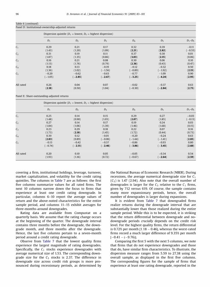
covering a firm, institutional holdings, leverage, turnover,market capitalization, and volatility for the credit ratingquintiles. The columns in Table 7 are as follows: the firstfive columns summarize values for all rated firms. Thenext 10 columns narrow down the focus to firms thatexperience at least one credit rating downgrade. Inparticular, columns 6–10 report the average values ofreturn and the above-noted characteristics for the entiresample period, and columns 11–15 exhibit averages forthree-months-around downgrades.

Rating data are available from Compustat on aquarterly basis. We assume that the rating change occursat the beginning of the quarter. The downgrade intervalcontains three months before the downgrade, the down-grade month, and three months after the downgrade.Hence, the last five columns pertain to a seven-monthperiod around a credit rating downgrade.

Observe from Table 7 that the lowest quality firmsexperience the largest magnitude of rating downgrades.Specifically, the C1 stocks experience downgrades withaverage numerical size of 1.53. The corresponding down-grade size for the C5 stocks is 2.37. The difference indowngrade size across credit risk groups is more pro-nounced during recessionary periods, as determined by

the National Bureau of Economic Research (NBER). Duringrecessions, the average numerical downgrade size for C1

(C5) is 1.47 (2.94). Also note that the overall number ofdowngrades is larger for the C5 relative to the C1 firms,given by 712 versus 619. Of course, the sample containsmany more expansionary periods, hence, the overallnumber of downgrades is larger during expansions.

It is evident from Table 7 that downgraded firmsrealize returns during the downgrade interval that aresubstantially lower than those realized during the entiresample period. While this is to be expected, it is strikingthat the return differential between downgrade and no-downgrade periods crucially depends on the credit risklevel. For the highest quality firms, the return differentialis 0.72% per month ½1:18� 0:46�, whereas the worst-ratedfirms record a much larger difference of 9.35% per month½�0:41� ð�9:76Þ�.

Comparing the first 5 with the next 5 columns, we notethat firms that do not experience downgrades and thosethat do, have similar firm characteristics. To illustrate, thedispersion measure ranges from 5.59 to 27.38 using theoverall sample, as displayed in the first five columns.The corresponding figures for the sample of firms thatexperience at least one rating downgrade, reported in the

ARTICLE IN PRESS

Table 7Analysis overall and around rating downgrades

Each month t � 1, all S&P rated stocks within a given subsample are divided into quintiles based on their credit rating. We exclude stocks priced below

$5 at the end of month t � 1. Each set of five columns reports, for various subsamples of firms, the time-series average of the cross-sectional mean

characteristic at time t for each credit rating quintile. The cut-off points for the rating quintiles, C1 (best-rated quintile), C2, C3, C4, and C5 (worst-rated

quintile), are held constant in all subsamples. The ‘‘3 months around downgrade’’ set of columns reports the average of the characteristic over months

t � 3 : t þ 3. Since rating data is available on a quarterly basis, the downgrade is assumed to happen during the first month of the quarter, t. All numbers

are in percentages unless noted otherwise. Dispersion is computed as the standard deviation of EPS forecasts divided by the absolute value of the mean

EPS forecast. Observations for dispersion are excluded when only one analyst EPS forecast is available or when the mean EPS forecast is zero. Revisions are

computed as the change from last month in mean analysts’ forecast for the next fiscal year, standardized by the absolute value of last month’s mean EPS

forecast. Earning surprise is defined as the actual EPS as of the report date minus last month’s forecasted EPS standardized by the absolute value of the

actual EPS. Analyst coverage is the number of analysts following the firm. Institutional holdings is the percentage of shares outstanding held by

institutions. Leverage is computed as the book value of debt for the most recent quarter, divided by the sum of the same book value of debt and the market

value of equity at the end of the previous month. Turnover is the percentage of shares outstanding traded in a particular month. Volatility is the standard

deviation of daily returns. The sample of all firms contains 12,312 companies over the period of July 1985–December 2003. The sample of firms with

downgrades contains 3,261 companies over the same period.

All firms Firms with downgrades

Overall 3 months around downgrade

Ratingquintile C1 C2 C3 C4 C5 C1 C2 C3 C4 C5 C1 C2 C3 C4 C5

Month-return obs.

Overall 41,426 53,082 52,980 55,231 52,315 30,799 38,549 37,273 35,004 31,303 2,965 4,013 4,010 4,204 3,485

Expansions 38,412 48,670 49,873 50,573 48,863 28,636 35,445 35,071 32,059 29,322 2,687 3,468 3,641 3,729 3,172

Recessions 3,014 4,412 3,107 4,658 3,452 2,163 3,104 2,202 2,945 1,981 278 545 369 475 313

Number of downgrades

Overall 619 730 669 698 712

Expansions 566 623 612 626 628

Recessions 53 107 57 72 84

Size of downgrades

Overall 1.53 1.60 1.69 1.65 2.37

Expansions 1.54 1.61 1.66 1.65 2.32

Recessions 1.47 1.44 2.16 1.62 2.94

Return 1.27 1.15 1.07 0.65 0.04 1.18 1.03 0.90 0.25 �0.41 0.46 �0.22 �1.92 �5.32 �9.76

Dispersion 5.59 8.32 12.97 19.89 27.38 6.04 9.09 14.35 23.09 32.17 11.69 20.28 27.34 40.73 47.54

Revision �0.68 �1.25 �2.14 �3.33 �4.00 �0.83 �1.47 �2.60 �4.15 �4.82 �3.01 �4.89 �7.95 �10.71 �9.05

Earning surprise �4.78 �8.60 �13.57 �17.13 �20.70 �5.95 �9.30 �13.31 �21.37 �22.56 �12.07 �23.22 �37.85 �40.36 �33.56

Analyst coverage 17.56 13.74 11.39 8.33 6.71 17.40 14.51 12.01 8.79 6.80 16.20 13.94 11.42 8.27 6.09

Institutional holdings 46.21 47.58 48.52 44.81 37.09 46.43 48.98 49.90 45.75 35.32 45.29 48.27 46.39 39.58 27.02

Leverage 22.24 27.42 33.06 40.08 43.96 23.29 28.28 34.14 42.89 47.73 29.94 34.12 43.27 54.62 59.86

Turnover 6.11 6.81 7.84 10.16 12.05 6.09 6.92 8.05 10.27 11.70 7.63 8.78 9.90 12.49 13.72

Size ($ billions) 6.66 3.60 2.12 0.97 0.60 6.71 3.92 2.35 1.06 0.59 5.33 2.96 1.55 0.57 0.34

Volatility 0.69 0.79 0.97 1.64 2.35 0.69 0.79 1.00 1.70 2.46 0.91 1.19 1.74 2.97 4.37


next five columns, differ relatively mildly and vary from6.04 to 32.17. However, the reported measuresare substantially larger during periods of downgrades. Insuch periods, dispersion ranges from 11.69 to 47.54,almost twice as much relative to the averages for theoverall period. Similarly, volatility for all firms with(without) downgrades ranges from 0.69 to 2.46 (0.69 to2.35). During downgrade intervals, volatility is higher andvaries from 0.91 to 4.37. Perhaps not surprisingly,institutional investors diminish their holdings of firmsthat experience downgrades, especially of the worst-ratedfirms.

In sum, periods of credit rating downgrades arecharacterized by declining returns as well as much higheruncertainty about firm fundamentals, as indicated bydispersion, forecast revision, and earnings surprises. Thisfinding motivates a formal investigation of the role of

credit rating downgrades in explaining the relationbetween dispersion and future returns, which we conductbelow.

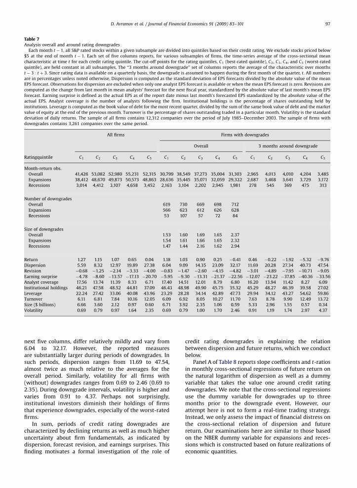
Panel A of Table 8 reports slope coefficients and t-ratiosin monthly cross-sectional regressions of future return onthe natural logarithm of dispersion as well as a dummyvariable that takes the value one around credit ratingdowngrades. We note that the cross-sectional regressionsuse the dummy variable for downgrades up to threemonths prior to the downgrade event. However, ourattempt here is not to form a real-time trading strategy.Instead, we only assess the impact of financial distress onthe cross-sectional relation of dispersion and futurereturn. Our examinations here are similar to those basedon the NBER dummy variable for expansions and reces-sions which is constructed based on future realizations ofeconomic quantities.

ARTICLE IN PRESS

Table 8Dispersion strategy payoffs excluding three-months-around downgrades (months t � 3 : t þ 3)

For Panel A, we run monthly cross-sectional regressions of returns, rit , on a constant, the natural logarithm of dispersion Dt�1, a downgrade dummy, and

credit rating CRt�1:

rit ¼ at þ bt�1Characteristicsi;t�1 þ uit .

The downgrade dummy takes the value of one three-months-around rating downgrades (i.e., from t � 3 to t þ 3). Panel A presents the average slope

coefficients, bt�1, in the cross-sectional regressions, averaged across all months in the sample, and multiplied by 100. The t-statistics are the sample

t-statistics of these estimated coefficients. For Panel B, we first remove firms three-months-around rating downgrades (i.e., from t � 3 to t þ 3). Then for

each month t, all stocks rated by Standard & Poor’s are divided into 25 groups based on a sequential sort by five credit rating and five dispersion groups.

For each rating/dispersion group, we compute the cross-sectional mean return for month t þ 1. All returns are in percentages per month. t-statistics are

presented in parentheses (bold if indicating 5% significance). The sample consists of 3,261 companies over the period of July 1985–December 2003.

Panel A: Cross-sectional regressions of returns on dispersion and a downgrade dummy

LogðDt�1Þ dummyt�3:tþ3 CRt�1

1 �0.14

(�2.07)

2 �0.09 �1.47

(�1.37) (�11.49)

3 0.03 �1.50 �0.10

(0.56) (�11.59) (�3.59)

Panel B: Returns by sequentially sorted rating and dispersion groups


D1 D2 D3 D4 D5 D1–D5

C1 1.46 1.29 1.34 1.36 1.40 0.06

(4.81) (4.34) (4.67) (4.60) (4.39) (0.29)

C2 1.41 1.25 1.40 1.39 1.36 0.05

(4.68) (4.22) (4.56) (4.46) (3.96) (0.24)

C3 1.31 1.26 1.30 1.42 1.23 0.08

(4.32) (4.03) (4.05) (4.35) (3.64) (0.41)

C4 1.32 1.17 1.17 1.13 1.14 0.18

(3.67) (3.20) (3.11) (3.05) (2.87) (0.79)

C5 0.86 0.56 0.48 0.58 0.50 0.36

(2.06) (1.29) (0.98) (1.26) (1.03) (1.17)

All rated 1.36 1.15 1.27 1.08 0.96 0.40

(4.56) (3.75) (3.95) (3.12) (2.46) (1.34)


Observe from Table 7 that the seven-month periodaround credit rating downgrades consists of only 18,677½2;965þ 4;013þ 4;010þ 4;204þ 3;485� observationsfrom the overall 255,034 ½41;426þ 53;082þ 52;980þ55;231þ 52;315� observations in our sample, apparentlya small fraction of only 7.32% of the sample observations.

Remarkably, this small fraction generates the disper-sion effect in the cross-section of future return. Toillustrate, the dispersion measure loses its statisticalsignificance when the downgrade dummy is added tothe cross-sectional regressions. The dispersion slope isequal to �0:09 with a t-ratio of �1:37. In contrast, thedowngrade dummy is statistically and economicallysignificant with a t-ratio of �11:49. When credit ratingis added as an additional explanatory variable thedispersion coefficient becomes 0.03 and the t-ratio 0.56.Thus, in the presence of a downgrade dummy and thelevel of the credit rating, the dispersion effect in the cross-section of return is virtually non-existent. The downgradedummy and credit rating are strongly significant witht-ratios given by �11:59 and �3:59, respectively. Thecross-sectional impact of forecast dispersion on future

returns is captured by credit rating level and by creditrating downgrades.

Next, we compute payoffs to dispersion strategiesduring no-downgrade periods using the 236,357 ½255;034� 18;677� observations. Panel B of Table 8 reportsdispersion profitability based on five credit ratingand five dispersion groups. Strikingly, implementingdispersion strategies during no-downgrade periodsgenerates profits that are statistically insignificant acrossall credit rating groups. The dispersion payoffs rangefrom 6 to 36 basis points per month, all of which areinsignificant.

To get an additional perspective about the impact ofrating downgrades on dispersion profitability we plot inFig. 2 the wealth accumulated by taking long (short)positions in stocks with low (high) dispersion in analysts’earnings forecasts starting from October 1985 but exclud-ing from the analysis periods around downgrades. Invest-ing $1 in dispersion strategies implemented among thehighest quality stocks (C1) yields a payoff of $1.14 inDecember 2003. The corresponding payoff is $1.62 whenthe investment universe is composed of low quality stocks

ARTICLE IN PRESS

198512 198812 199112 199412 199712 200012 200312

0

1

2

3

4

5

6

Wea

lth

pro

ce

ss

Year

C1

C3

C5

Fig. 2. Wealth process of dispersion strategy in non-downgrade periods. We repeat the strategy outlined in Fig. 1, after excluding return observations of

stocks three-months-around rating downgrades (t � 3 : t þ 3). Each month t, all stocks rated by Standard & Poor’s that do not have downgrades in the

preceding three months or the subsequent three months are divided into quintiles based on credit rating. For each credit rating quintile, we further sort

stocks into quintiles based on dispersion and assume we are $1 long in the lowest dispersion quintile (D1) and $1 short in the highest dispersion quintile

(D5) and hold these positions for one month. This dispersion strategy is followed from October 31, 1985 until December 31, 2003, and includes a total of

3,261 rated stocks. The plot illustrates the wealth processes for rating quintiles C1 (highest-rated), C5 (lowest-rated), and the middle quintile C3.

−36 −30 −24 −18 −12 −6 0 6 12 18 24 30 36

−0.08

−0.07

−0.06

−0.05

−0.04

−0.03

−0.02

−0.01

0

0.01

0.02

Months around downgrade

Month

ly r

etu

rn

C5

C1

Fig. 3. Returns around rating downgrades. Each month t, stocks with available S&P ratings in Compustat are divided into rating quintiles. Within each

quintile, we find stocks that have been downgraded that month and compute their equally weighted average returns over each month from t � 36 to

t þ 36. We repeat this every month. The figure presents these average monthly portfolio returns for the best (C1) and worst (C5) rated quintile portfolios

around periods of rating downgrades. Month 0 is the month of downgrade. Since S&P ratings are available in Compustat on a quarterly basis, we assume

the downgrade happens in the first month of the quarter, t ¼ 0. The sample consists of 3,261 companies over the period of July 1985–December 2003.


(C5). Recall from Fig. 1 that the corresponding payoffs are$1.28 and $4.82, respectively, when periods of down-grades are included.

Whereas Fig. 2 undertakes the calendar-time perspec-tive, it is also useful to examine the downgrade effect froman event-time perspective. Fig. 3 plots monthly returnsaround credit rating downgrades. The overall evidenceshows that returns on high quality stocks (C1) displayvirtually no sensitivity to deteriorating credit conditions.In contrast, prices of low quality stocks (C5) decreasesubstantially during periods of worsening credit condi-tions. At the same time, Fig. 4 displays that analystdispersion of C5 stocks rises drastically, while that of C1

stocks is almost unaffected by the downgrade. This pricedrop accompanied by an increasing forecast dispersion in

high credit risk stocks around downgrades ultimatelygenerates the dispersion effect in the cross-section ofreturns.

As shown throughout, credit rating downgrade periodsare characterized by substantial price drops among low-rated stocks. An essential question remains: are worsen-ing credit conditions merely proxying for negative pastreturns? To make sure that credit rating changes areeconomically meaningful, we implement dispersion stra-tegies for different subsamples similar to Table 4, butprogressively eliminate loser stocks (rather than low-rated stocks) from the analysis.

Table 9 reports the results. Eliminating the 4–52%of the largest negative past return stocks yields aninvestment universe with statistically and economically

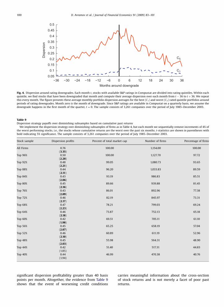
ARTICLE IN PRESS

−36 −30 −24 −18 −12 −6 0 6 12 18 24 30 36

0.05

0.1

0.15

0.2

0.25

0.3

0.35

0.4

0.45

0.5

Months around downgrade

Dis

pers

ion

C5

C1

Fig. 4. Dispersion around rating downgrades. Each month t, stocks with available S&P ratings in Compustat are divided into rating quintiles. Within each

quintile, we find stocks that have been downgraded that month and compute their average dispersion over each month from t � 36 to t þ 36. We repeat

this every month. The figure presents these average monthly portfolio dispersion averages for the best (C1) and worst (C5) rated quintile portfolios around

periods of rating downgrades. Month zero is the month of downgrade. Since S&P ratings are available in Compustat on a quarterly basis, we assume the

downgrade happens in the first month of the quarter, t ¼ 0. The sample consists of 3,261 companies over the period of July 1985–December 2003.

Table 9Dispersion strategy payoffs over diminishing subsamples based on cumulative past returns

We implement the dispersion strategy over diminishing subsamples of firms as in Table 4, but each month we sequentially remove increments of 4% of

the worst performing stocks, i.e., the stocks whose cumulative returns are the worst over the past six months. t-statistics are shown in parentheses with

bold indicating 5% significance. The sample consists of 3,261 companies over the period of July 1985–December 2003.


All Firms 0.76 100.00 1,154.00 100.00

(3.35)

Top 96% 0.50 100.00 1,127.70 97.72

(2.28)

Top 92% 0.48 99.05 1,080.73 93.65

(2.21)

Top 88% 0.44 96.20 1,033.83 89.59

(2.11)

Top 84% 0.43 93.19 986.83 85.51

(2.06)

Top 80% 0.45 89.66 939.88 81.45

(2.16)

Top 76% 0.43 86.01 892.96 77.38

(2.09)

Top 72% 0.46 82.19 845.97 73.31

(2.17)

Top 68% 0.47 78.21 799.03 69.24

(2.23)

Top 64% 0.46 73.87 752.13 65.18

(2.18)

Top 60% 0.42 69.51 705.11 61.10

(1.98)

Top 56% 0.45 65.25 658.19 57.04

(2.07)

Top 52% 0.46 60.89 611.19 52.96

(2.10)

Top 48% 0.45 55.98 564.31 48.90

(2.03)

Top 44% 0.42 51.40 517.31 44.83

(1.85)

Top 40% 0.44 46.99 470.38 40.76

(1.94)


significant dispersion profitability greater than 40 basispoints per month. Altogether, the evidence from Table 9shows that the event of worsening credit conditions

carries meaningful information about the cross-sectionof stock returns and is not merely a facet of poor pastreturns.

ARTICLE IN PRESS


4. Conclusion

This paper establishes a link between credit rating andthe profitability of trading strategies that are based ondispersion in analysts’ earnings forecasts. The empiricalfindings are based on a sample of 3,261 NYSE, Amex, andNasdaq firms rated by S&P over the July 1985–December2003 period. The selected sample is representative incapturing the negative relation between dispersion andfuture returns as well as the negative relation betweencredit risk and future returns, both of which have beenperceived to establish anomalous patterns in the cross-section of returns.

Our analysis shows that the documented profitabilityof dispersion strategies is driven by the worst-rated firms,which account for less than 5% of the overall marketcapitalization of rated firms. In contrast, dispersionprofitability is non-existent among higher quality firms.Even within the small universe of low-rated firms, anadjusted dispersion measure that excludes the creditrisk component has no statistical power to predict thecross-section of future returns. Moreover, implementingdispersion strategies using credit rating-adjusted returnsyields payoffs that are economically small and statisticallyinsignificant. Firm size, leverage, volatility, past returns,institutional ownership, and turnover, all of which havebeen proposed by previous work to explain the disper-sion–return relation, do not capture the impact of creditrating on dispersion profitability.

Financial distress drives the dispersion effect. Inparticular, the negative cross-sectional relation betweendispersion in analysts’ earnings forecasts and future stockreturns prevails only during periods of credit ratingdowngrades. In such periods, prices of low-rated stocksdecline substantially and the uncertainty about firmfundamentals (measured by analyst forecast dispersion,forecast revisions, or earnings surprises) rises consider-

ably. In the remaining periods, which consist of about92.68% of the overall observations in our sample, thedispersion–return relation is insignificant.

References

Amihud, Y., 2002. Illiquidity and stock returns: cross-section and timeseries effects. Journal of Financial Markets 5, 31–56.

Avramov, D., Chordia, T., Jostova, G., Philipov, A., 2006. Credit ratings andthe cross-section of stock returns. Working Paper, University ofMaryland.

Avramov, D., Chordia, T., Jostova, G., Philipov, A., 2007. Momentum andcredit rating. Journal of Finance 62, 2503–2520.

Campbell, J.Y., Hilscher, J., Szilagyi, J., 2008. In search of distress risk.Journal of Finance 63, 2899–2939.

Carhart, M.M., 1997. On persistence in mutual fund performance. Journalof Finance 52, 57–82.

D’Avolio, G., 2002. The market for borrowing stock. Journal of FinancialEconomics 66, 271–306.

Dichev, I.D., 1998. Is the risk of bankruptcy a systematic risk? Journal ofFinance 53, 1131–1147.

Dichev, I.D., Piotroski, J.D., 2001. The long-run stock returns followingbond rating changes. Journal of Finance 56, 55–84.

Diether, K.B., Malloy, C.J., Scherbina, A., 2002. Difference of opinion andthe cross-section of stock returns. Journal of Finance 57, 2113–2141.

Fama, E.F., French, K.R., 1993. Common risk factors in the returns onstocks and bonds. Journal of Financial Economics 33, 3–56.

Fama, E.F., MacBeth, J.D., 1973. Risk, return, and equilibrium: empiricaltests. Journal of Political Economy 81, 607–636.

Griffin, J.M., Lemmon, M.L., 2002. Book-to-market equity, distress risk,and stock returns. Journal of Finance 57, 2317–2336.

Hand, J.R.M., Holthausen, R.W., Leftwich, R.W., 1992. The effect of bondrating agency announcements on bond and stock prices. Journal ofFinance 47, 733–752.

Johnson, T.C., 2004. Forecast dispersion and the cross-section of expectedreturns. Journal of Finance 59, 1957–1978.

Merton, R.C., 1974. On the pricing of corporate debt: the risk structure ofinterest rates. Journal of Finance 29, 449–470.

Moskowitz, T.J., Grinblatt, M., 1999. Do industries explain momentum?Journal of Finance 54, 1249–1289.

Sadka, R., Scherbina, A., 2007. Analyst disagreement, mispricing, andliquidity. Journal of Finance 62, 2367–2403.

Vassalou, M., Xing, Y., 2004. Default risk in equity returns. Journal ofFinance 59, 831–868.

Zhang, X.F., 2006. Information uncertainty and stock returns. Journal ofFinance 61, 105–136.

dispersion in analysts’ earnings forecasts and credit rating

Documents