$-'HtOrarlimRmrctrMh[inSford

DISPERSAL OF DREDGED MATERIAT

Application of short term model forcohesive sediments

A P Diserens, BScE A De1o, BSc, PhD, CEng, I , I ICE, UIWEII

Report SR 210May 1989

Registered Office: Hydraulics Research Limited,Wallingford, Oxfordshire OXIO 8BA.Telephone: O49l 35381. Telex: 84g552

CONTRACT

This report. describes work funded by the Department of the Envj-ronment underResearch contract PECD 7/7/164 for vhich the nominated officer wasMr C E Wright. It is published on behalf of the Department of theEnvironment, but any opinions expressed in the report are not necessarilythose of the Funding Department. The work was carried out byMr A P Diserens in Dr E A Delo's Section in the Tidal- Engineering Departmentof Hydraulics Research, Wallingford under the management of Mr M f' C Thorn.

@C.o*n copyright. l9B9

Published by permission of the Controller of Her Majestyrs StationeryOf f i ce .

ABSTRACT

There are two mal.n factors governlng the suitability of a site for thedisposal of dredged material. Flrst ly, short-term recycl ing of materialback into the dredged area nust be low enough for this method of disposal tobe cost effective. Secondly, the environmental impact nust be within anacceptable level.

To quantify the degree of short terrn re-cycling it is necessary to know thefate of the disposed naterial. In the past this has been done using tracerstudies to Look at the suitabil.ity of specific sites. However tracerstudies involve considerable organlzation which limlts the nrrrnber ofpositions that can be invegtlgated. Clearly a mathematical nodel which wllLpredict the fate of material disposed of at any given time and position wiLlenable rnore effective seLection and evaluetion of disposal sitel withrespect to term re-cycling.

This report details the application of a mathematical model for predictingthe short terrn dispersal of rmrddy dredged meterial. The aim was tocalibrate the model by simulating the distribution of deposited sediment onthe bed after one particuLar dlsposal er<periment and then verify the modelby using the sane pararneters to ej.nulate the deposited mass on the bed afteranother disposal oq>eriment.

Ttre short tern dispersaL rnodel is applicable to predicting the fate ofcohesive sediments either out-washed during aggregate dredging or dischargedby side-casting of dredged naterial. It is therefore a uEeful tool inassessing the approprlateness of proposed disposal sites in tK tidal. watersin connection with licence applications for the disposal of dredgedmaterial.

Existing field data were used from a study associated with the proposedenlargement of a dredged channel. This has involved monitoring-thedispersal of muddy dredged materlal, IabeLled with a radioactive tracer,from a floating pipe. Itre distrlbution of the sediment on the bed afterdisposal was determined by monitoring the radio-activity on the bed. Flowconditions and water depth were measured over the e:<perimental perLod.E : rpe r i nen tghadbeenca r r i edou tonbo th the f I oodandebb t i de i

Using the hydrodynamie data measured at the time of the study, the localbathymetry and the rate and duratlon of sediment input, the distribution ofthe disposed material on the bed was predicted using the nodel.

The model was calj.brated by optimising the settling velocity and thediffusion coefficients to simulate as closely as possible the distributionof deposited sediment on the bed produced by the ilood tide orperiment. Thesettling velocity anci the diffuEion coefficients in the x and y directionsfor the sediment were unknown parameters. Accordingly, estimated valueswere chosen for lnitial nodel runs, these values were modified to produce adistribuLion sirnilar to that found in the field survey.

In the course of the calibration runs it was found to be neeessary to modi.fythe equation for the rate of deposition to take into account the decrease insettling caused by horizontal flow. The model was also found to give more

satisfaetory results wj.th a constant floc settling velocity rather than asfiurction of suspended sediment concentration. Ttre nedian floc settlingvelocity was varied as part of the nodel optimising process.

The nodel was then verified by using the opti-rnised values of settlingvelocity and dlffuEion coefficients to sitnulate the ebb tide depositionplume.

The distribution of deposited sediment from the flood and ebb tideocperiments were sirmrLated within acceptable U.rnits using the opti.rnisedvalues. A slight deviatlon of the angle of, the ebb tide sirnulation waEthought nost likely a result of the lfunitations of the hydrodynanic datacollected at the ti-rne of the orperinent.

CONTENTS

1 INTRODUCTION

2 THE MATHEMATICAL UODEL

2.L Descript ion of physical processes2.2 Solutj-on technique2,3 Calculat ion of distr ibut ion of suspended sol ids

concentration and mass on bed

3 FIELD DATA

3.1 Background to study3.2 Hydrodynamic data and bathymetry3.3 Tracer study procedure3.4 Tracer study results

4 MODEL APPTICATION

4.L Model input and output4.2 Interpretat ion of f ie ld data4.3 Method of analysis of results4.4 Cal ibrat ion and veri f icat ion4.5 Comparison of model output with field data

5 CONCLUSIONS

6 REFERENCES

TABLES

Page

I

3

35

A

6

67B9

9

9101 1L2L4

15

77

I234

Conversion of iso-activity lines to mass per square metreFinal parameters used in rnodelComparison of field data with model results, flood tideComparison of field data with model results, ebb tide

FIGURES

Field study area - Ban DonHydrographic field dataBathymetry of flood tide plume model areaBathynetry of ebb tide plume model areaFlood tide plune field data distribution of mass on bedEbb tide plume field data distributi_on of mass on bedTotal activity against area flood tide plumeTotal activity against area ebb tide plumeFlood tide plume model results distribution of mass on bedEbb tide plume rnodel results distribution of mass on bedComparison of areas within contour bands flood tide plumeComparison of masses within contour bands flood tide plumeCompari-son of areas within contour bands ebb tide plume (inside modelboundary)

L4 Comparison of masses within contour bands ebb tide plume (inside modelboundary)

I234567B91011L213

PLATE

I Inject ion of t racer

APPENDIX A

Notes on running the model

INTRODUCTION

The increase in size and draft of shipping in recent

years has resulted in an i-ncrease in dredging

operations throughout the world. Since dredging

operations are expensive, methods are continually

being sought to increase cost effectiveness. For

economic reasons much of the dredged material from

these operations is disposed of back into the marine

environment. With the increase in dredging operations

new sites for marine disposal are being sought and

exist ing si tes are being reassessed.

There are two main factors governing the suitability

of a site for the disposal of dredged material.

Firstly, short-term recycling of material back into

the dredged area must be 1ow enough for this method of

disposal to be cost effective. Secondly, the

environmental impact must be within an acceptable

leve l .

To quantify the degree of short term re-cycling it is

necessary to know the fate of the disposed material.

In the past this has been done using tracer studies to

look at the suitability of specific sites. However

tracer studies involve considerable organization rchich

Iimits the number of positions that can be

investigated. Clearly a mathematical model which

could predict the fate of material disposed of at any

given time and position would enable more effective

minimisation of short term recycling.

Due to the r is ing pol i t ical importance of

environmental issues, the affects of the disposal of

polluted waste on the marine environment are being

increasingly invest igated. The disposal of dredged

material is no except.ion. Sediments dredged from

channels passing through industrial areas are usually

high in pollutants, particularly heavy metals. The

prediction of the movement of these sediments woufd

also be of considerable benefit when assessJ,ng the

environmental implications of proposed disposal

schemes.

The objective of the work was to create an economic

means of predicting the short term dispersion of

disposed dredged material in tidal waters. This

report details the application of a short term

dispersal model previously developed by HydrauLics

Research (Ref 1). The aim was to simulate the

dispersal of muddy dredged material- measured during a

field study in Ban Don Bay, Ihailand. The field data

were collected during a study associated with the

proposed enlargement of a dredged channel in the bay.

This involved monitoring the dispersal of dredged

material, labe11ed with a radioaetive tracer,

discharged directly frorn a dredger. The distribution

of the sediment on the bed after disposal was found by

monitoring the radio-activity on the bed. Flow

conditions and water depth were measured over the

experimental period. Experiments were carried out on

both the flood and ebb tides.

Using the hydrodynamic data measured at the tine of

the study and the local bathyrnetry, the distribution

of the disposed material on the bed was predicted

using the mathematical rnodel. The model was first

calibrated on the flood tide deposition ph:me. The

settling velocity and dispersion coeffi-cients were

adjusted to give a distribution of deposited sediment

on the bed as similar as possible to that found in the

field. The model was then verified by using the

settling velocity and dispersion coefficients found in

Lhe calibration to simulate the ebb tide deposition

plune.

2 THE MATHEMATICAL

MODEL

2. I Descr ip t ion of

physical processes

The dispersion and deposition of suspended solids

depends mainly on advection by currents, the settling

of the sediment and the diffusion due to natural

turbulence in the flow.

fn a turbidity cloud generated from a surface source,

the horizontal component of velocity of a suspended

particle is determined by the flow velocity of the

water into which it falls. This is known as

advection.

The vertical component of velocity of a suspended

solid particle depends both on the characteristics of

the flow, such as turbulence, and those of the

sedj-ment, such as size, shape and density of the

particles and the tendency of the sediment to

flocculate. The settling velocity reflects these

propert i -es.

The spread of material away from a dense cloud is'

known as diffusion. Longitudinal diffusion is eaused

by the difference in velocities of the water at the

surface and at the bed. Lateral diffusion det,ermines

the rate of spread of the cloud due to natural

turbulence in the moving current. In an estuary, the

scale of turbulent eddies may be lateral ly restr icted,

so the cloud may form a long thin ribbon which spreads

sideways only slowly.

These physical processes can be described by the

combination of three equations. These include a

partial differential equation for the spread of

material from a point source, an equation for the

loss of material from suspension due to settling, and

an equation for the movement of material by the flow.

The solution is simplified by assuming that flow

velocity, depth, and turbulent diffusion remain

constant over the length of the plume. It is aLso

assumed that the flow is uni-directional, parallel to

the x-direction and that the material is fulty mixed

throughout the depth from the point of release. Thre

basic equation then becomes:

?c*9(uc)-o l4-o ? ' :*5f"-"_l-o (1)a t ' 0 x " x 0 x 2 " y 6 y , d r - - e ,

where:

c = depth averaged concentration (kgm-3)

d = water depth (m)

x,y = co*ordinate directions parallel and normal to

the flow (m)

u = f low veloci ty in the x direct ion ms-l

D-, ,D__ = Dif fusion coeff ic ients in the x and yx - ydirect ions respect ively (mzs-r)

W_ = effect ive fal l veloci ty (ms-l)s

"" = depth averaged background concentration

(kgm- I )

| = t i rne(s)

This partial differential equation is the continuity

equation for the spread of material from a point

source. The terms represent the rate of change of

concentrat ion with t ime, the rate of decrease of

concentration per unit volume by advection,

Iongitudinal di f fusi-on, lateral di f fusion and loss of

mater ial f rom suspension due to sett l ing

respect ively.

2.2 Solut ion Technique

Equation (1) can be solved for a point release of

material into flowing water. This gives .X"fi;;

distribution of suspended mass at any time. The

centre of the plume moves downstream at the velocity

of the water with decreasing concentration as a result

of diffusion and settling. However this solution is

Iimited by the constraints of constant hydrodynamic

parameters (current velocity and direction, settling

rate and water depth).

To develop a model which would accurately predict the

dispersion of material in tidal waters, where the

hydrod;manic parameters are constantly changing,

the basic solution is applied repeatedly over short

time steps. The hydrodynamic parameters are re-set

each time step to represent field conditions. The

water depth at the position of greatest concentration

is taken as representative of the area and is used in

the solution of the equation. the dispersion of the

plume of dredged material is given by the convolution

of discret ised analyt ic solut ions.

The area for which a solution is required is divided

up into a grid of cells. The analytic solution i5

then solved in terms of mass at the centre of each

cell. It is assumed that the mass is evenly

distributed throughout the depth in each ee1l.

The combination solution is made up by treating each

cell as a point source. The distribution of the mass

originating in each ce}l after one time step is

calculated using the analytic solution. The

distr ibut ion is the same for al l ceI ls, in terms of

mass fraetion, since the dispersion coefficients and

hydrodynamic parameters are assumed to be constant

throughout the area. The mass in each cell at the end

2 .3 Calculat ion of

suspended solids

concentration and

mass on bed

FIETD DATA

Background of study

of a time step can then be calculated by summing the

contributions from all other cells. This mass is

subseguently used as the magnitude of the point source

at the start of the next time step.

Discretising the solution leads to small discrepancies

in the total mass. A correction is made for this when

calculating the deposited mass during each time step

to conserve total mass.

The concentration at the centre of each cell at the

end of a given time step, can be calculated frorn the

mass in the eell and the depth of the ce1I.

The flux of material settling to the bed in a cel1 is

directly proportional to the suspended solids

concentration at that time and the settling velocity

of the material. Since the suspended solids

concentration in a cel1 changes over a time step the

average of the concentrations at the start and the end

of the time step is used.

The f ield data used for s imulat ion of the dispersal of

dredged material was obtained by Hydraulics Research

during a study connected vith the development of

coastal ports in Thai land (Ref 2).

I t was proposed to increase the size of the access

channel in Ban Don Bay to enable passage of larger

3 .1

3.2 Hydrodynanic data

and bathyrnetry

vessels to the port (Fig 1). The scheme entai led

increasing the depth of the channel to a depth of 4m

and a width of 60m and extension of the channel out to

a natural water depth of 4m. The original access

channel followed a bearing of 30o from the mouth of

the Tapi river to beyond Ko Prap island from which the

new extension would take a line due north to deeoer

water.

Discharge of material to extensive adjacent banks, via

a floating pipe, was the economically favoured rnethod

of disposal. To determine the fate of material

discharged in this way a radioactive tracer study was

corrnissioned. Ttris tracer study included experiments

on both the flood and ebb tides. The activity of the

bed in the area around the point of discharge was

monitored after disposal to determine the distribution

of the discharged material.

Tide levels throughout the experimental period were

obtained from the tidal recording station at Ko Prap

island (see Fig 1). During each disposal per iod

measurements of current speed and direction were faken

lm above the bed at 20 minute intervals, using a

Braystroke directional current meter. Measurements of

wind speed and estimates of wave heights were also

recorded. The results of these measurements are shown

in Figure 2.

The bathymetry was estimated from the admiralty

chart of the region. The bathymetry used in the model

simulations is shown in Figures 3 and 4.

3 .3 Tracer study

procedure

For the tracer study Gold 198 was chosen, since its half

life of 2.7 days was suitable for the planned duration

of the study. In addition the attenuation of its

principle emission (garrna radiation of 0.412 Mev) in

marine sediments is sufficiently low that the measured

activi.ty is not affected by overlying sediment.

A sanple of sedirnent from the area was cleaned and

labelled with the radioactive isotope immediately prior

to injection. The 1abel1ed sediment was then released

with the dredged material at a constant rate during each

disposal period. Subsequently the radioactivi-ty of the

bed in the vicinity of the disposal site was surveyed

using a radiation detector towed along the bed. The

radiation readings were corrected for bed background and

isotope decay.

The site of the injection area was rnid way along the

proposed channel extension (see Figure 1). In order to

examine the behaviour of dredged material discharged on

both the flood and ebb flow two injections were made

either side of high water on 24 March 1982. The actual

times of the injections are shown in Figure 2. The'

flood injection was approximately 2.5h before high water

and the ebb injection approximately 2.5h after high

water. The duratj-on of each injectj-on period was

approximately 30 min in both e:cperiments. The density

of the slurry was 1100 kgm-r and the pumping rate was

100 m3h-1. The bed was surveyed I day, 3 days and

9 days after in ject ion.

3.4 Tracer study

results

4 . 1

MODEL APPTICATION

Model input

and output

The results of the bed activity surveys were plotted

on previously prepared charts. From these, contour

plots of iso-activity were drawn. Since the results

of the survey after I day were the most comprehensive

only these results have been used in this report

(F igures 5 and 6) .

The flood deposition plume extended approximately

1000m landward and had a maximr:rn width of about 40Om.

The ebb depositi.on plume extended approximately 7 km

seaward and had a width of between l00m and 300m

throughout its length. The disparity in the tracer

extent is in part a consequence of the stronger

velocities of the ebb flow and in part because the

injections did not coincide with the mid flood and

mid ebb flows. The injection after high water was

followed by 5h of ebb flow, whereas, that before high

water rras followed by only 1.5h of flood flow.

The iso-activity lines showed that the highest

activity occurred at the point of injection, the

activity decreasing eqponentially with distance from

this point.

The model was modified from that used previously

(Ref 1) to al1ow the sediment to be input as a

specified mass over a number of time steps

corresponding to the period of injection. This enabled

fluctuations in flow direction and velocity over the

inject ion period to be nodel led more accurately. The

4.2 Interpretation

field data

program was run using the hydrodlmamic data collected

in the field and the actual bathymetry of the area. A

grid size of 30m by 30m was used in the model which

covered an area of 1500m by 1500m.

Ttre output from the model was i.n the form of tables

and contour plots of both the suspended concentrations

and tota] mass deposited in each cell. Each set of

output was sent to a file for future inspection and

analysis.

o f

The field data results were in the form of a contour

plot of iso-activity contour lines. In order to

enable a direct comparison between the model output

and the field results it was necessary to determine

the equivalent mass per square metre of the iso-

activity contour lines. Because the counts per minute

on the bed was directly proportional to mass this

could be found from the ratio of total mass to total

activity.

Since there appeared to be an exponential decrease in

activity with increasing distance from the injectlon

point the following equation was used to approximate

the total activity in each contour band:

Ri = Ai 10 e>rp { (1ogr . + Logr .* r ) /2}

where

total activity in contour band i (cpm

area i-n contour band i (mz )

activity of contour leve1 i (cpm)

( 2 )

R .l_

A .l_

rl-

10

m ? )

This reLationship held for all contour bands except

the 500 cpm to 1000 cpm eontour band of the ebb tide

plume which extended in a long thin plume beyond the

model limits. The activity in the area beyond the

model limits was not decreasing sq)onential1y. Hence,

for the area up to the model limits equation (2) was

used and for the area beyond the model limits it rras

assumed that the activity was constant at 500 cpn.

The amount of activity within the highest contour was

estimated by assuming a peak activity.

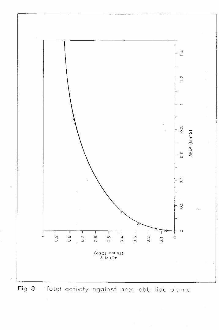
The total activity within each contour is given in

Table 1. A graph of cumulative acti-vity against area

for each plume (Figs 7 and 8) enabled the amount of

activity outside the range of the lowest contours to

be found by extrapolation.

The total mass corresponding to the total activity was

calculated from the dry density, the pumping rate, and

the duration of sediment input.

The mass per uni-t area of material on the bed may be

assumed to be proportional to the counts per minute in

the same ratio as total mass to the total activity.

This relationship was used to find the mass per square

metre corresponding to the iso-activity lines of fhe

field results. These vaLues were then specified for

the contours levels in the model output. This enabled

direct comparison of the extent and position of the

plume on the model output with the field data.

4.3 Analysis of results

The array of values corresponding to the masses on the

bed at the time of the model output were processed to

calculate the area and masses inside each contour

band.

1 1

4 .4 Calibration and

verifi.cation

The area inside each contour band was calculated by

multiplying the number of cells with values vithin

each band by the area corresponding to the celI si-ze,

900 m2. The total mass within each contour band was

calculated using the same method as the field data,

substituting mass for activity in equation 2. This

enabled a direct graphical comparison of the

distribution of mass between the field results and the

model output.

The model was calibrated by optirnising the settling

velocity and the diffusion coefficients to sirrulate as

closely as possible the distribution of deposited

sediment on the bed found in the field survey. The

settling velocity and the diffusion coefficients in

the x and y directions for the sediment were unknolrn

parameters. Accordingly, estimated values were chosen

for initial model runs and these values were modified

to produce a distribution sinilar to that found in the

field survey. A sma1l number of runs were undertaken

to ensure that the model was not over sensitive to

grid size or time step.

In the course of the calibration runs it was found to

be necessary to nodify the equation for the rate of

deposition to take into account the decrease in

settling caused by horizontal flow. The horizontal

flow generates a shear stress on the bed. A critical

bed shear stress exists, rbc, above which there is no

deposit ion. At shear stresses below this cr i t ical

value deposit ion wi l l occur (Ref 3).

The shear stress at the bed vas calculated from the

horizontal velocity lm above the bed using the

equat ion proposed by Sternberg (Ref 4),

L2

r b = 0 . 0 0 3 p * U 1 , ( 3 )

where

tO = bed shear stress (Nm-z)

po, = f lu id density (kgm-r)

U1 = veloci ty lm above bed (ms-l)

Although refinements of this relationship exist

(Ref 3), this equation was chosen because of its

simplicity. The accuracy of the bed shear stress

calculated in this way was adequate for the

appl icat ion.

The amount of deposition at shear stresses below the

critical value is approxi-mated by the following

equation

Ws = Wuo (1 - tb l .b " )

where

Ws = Effect ive fal l veloci ty (ms-1)

Wso = median sett l ing veloci ty of f locs (ms-1)

.b = bed shear stress (Nn-z)

tb" = cr i t ical bed shear for deposit ion (Nm-z)

The model was found to give more satisfactory results

vith a constant floc settling velocity rather than

with settling velocily a function of suspended

sediment concentration used previously. The median

f loc sett l ing veloci ty was var ied as part of the model

opt imising process.

The model was then verified by using the optimised

values of sett l ing veloci ty and di f fusion coeff ic ients

t,o simulate the ebb tide deposition plume.

( 4 )

I J

The parameters used in the fi-na1 model runs are given

in Table 2.

4.5 Compari-son of model

outpul with field

data

fhe contour plots of the distribution of deposited

sediment produced by the optimised parameters are

shown in Figures 9 and 10. The simulation of the

flood injection produced a deposited mass plume 1000m

long and 300rn wide with a bearing of approximately

I80o for iLs long axis. The sjmulation of the ebb

injection produced a long thin plume of between 100m

and 3O0m wide and spread beyond the model limits, over

1500m in length. The long axis of the ebb deposition

plume was orientated at a bearing of approximately

450 .

The contour plots of tbe model output were compared

visually with the field survey results. Both the

extent of the deposition plume and the relative

positions and shape of the contours within the ph:me

were compared with the field results. In addition the

distribution in terms of area and masses lrithin each

contour band was compared. This data is tabulated

(Tables 3 and 4) and shown in the form of histograrns

(Figs 11 to 14) for both the f lood t ide and ebb t ide

plurnes.

The f lood t ide sj .nulat ion (Fig 9), used for

cal ibrat ing the model, compared closely in size and

posit ion with the f ie ld data (Fig 5) in size,

distr ibut ion and or ientat ion.

The distribution of the deposited sediment within the

flood tide plume in the model results in terms of area

and mass (Figs 11 and L2), agteed quite closely

1 t ,

CONCLUSIONS

with the field data. The area within each contour

band increased as the mass per unit area on the bed

decreased. The distribution in terms of mass followed

a dj-fferent pattern. The mass increased to a peak

with the largest proportion of the mass in the

0.075-0.038 kgrn-2 band. The proport ion of the nass

decreased with decreasing mass per unit area. The

t,rends were similar for both the field and model

results. The mass in each contour band agreed to

within 10% of the total mass.

The simulation of the ebb tide disposal used to

verify the model (Fig L0) did not give quite such a

close match with the fietd data (Fig 6). Ttre bearing

of the axis of the plume differed by about l0o from

the field data. fhe width and the distri"bution within

the plume did however compare well with the field

data.

The distribution of the sediment within the sirnulated

ebb tide plume (Figs 13 and 14) gave good agreement

with the field data. The area within each contour

band increased more markedly than that of the flood

tide plume as the mass per unit area decreased. Ihe

amount of mass in each contour band also increased

with decreasing mass per unit area. The distribution

of mass was broadly similar for both the field and

model results. The mass in each contour band asreed

to within 127. of the total mass.

1. The model aimed to simulate the short term

dispersal of dredged mater ial measured during a

field study in Ban Don Bay, Thailand. This study

entai- led monitor ing of the dispersal of dredged

material , label led with a radioact ive tracer.

Tide levels and flow conditions were measured

1 5

2 .

during the disposal period. The or.periments were

carried out on both a flood and ebb tide at two

pos i t ions .

The mathematical model took into account the

hydrodynamic field data, the local bathymetry and

the rate and duration of dredged material

disposal. It was calibrated by optirnising the

coeffi-cients of dispersion and the apparent

settling velocity of the sediment to produce a

distribution of deposited sediment as similar as

possible to the flood tide disposal field

resu l ts .

The model was verified by using the optirnised

eoefficients for diffusion and apparent settling

velocity, from the calibration, to simulate the

distribution of sedi-raent on the bed from the ebb

tide injection.

The distribution of deposited sediment from the

flood and ebb tide experiments (Figs 5 and 6)

were sirm.rlated within acceptable limits (Figs 9

and l0) using the optimised values. The sJ-ight

deviation of the angle of the ebb tide sirmrlation

is most likely a result of the linitations of the

hydrod5mamic data collected at the time of the

experiment.

3 .

4 .

16

REFERENCES

1 .

2 .

J .

4 .

Delo E A, Ockenden M C, Burt T N. "Dispersal

of dredged material: Mathematical model of a

plumer' , Hydraul ics Research, Wal l ingford,

England. Report No SR 133, June 1987

Hydraulics Research. "Thailand coastal ports

project: Navigation channel improvements at the

port of Ban Don - radioactive tracer aq>eriments

to examine the disposal of dredged spoilfr,

Hydraulics Research, Wallingford, England.

Report No EX 1055, June 1982

DeIo E A. I'Estuarine muds manualtr. Hydraulics

Research, Wallingford, England. Report No SR 164,

February 1988

Sternberg R W. I'Predicting initial motion and

bed load transport of sediment particles in the

shallow marine environmentr'. Shelf Sediment

Transport . pp 61-82

I 7

TABLES.

TABLE I : Conversion of isoactivity lines to mass per square metre

FLOOD TIDE PLUME

TOTAL MASS DISPOSED = 6600kg

/f = ESTII{ATED VALUES

RADIO

ACTIVITY

(cpn)

<500

500

1000

2000

5000

10000

20000

>20000

RADIO

ACTIVITY

(cpn)

>500

500 a

s00 p

1000

2000

5000

10000

> 10000

RANGE

AREA

(rn2 )

637s0

56250

63r25

41875

L0625

l8 l 3

RANGE

AREA

(m2 )

428000

302s00

89300

43 100

10000

3 130

RANGE

ACTIVITY

(cpm m2)

/15 .0*1.0?

4 . 5 * 1 0 ?

8 . 0 x 1 0 6

2 . 0 * 1 0 6

3 . 0 * 1 0 8

I . 5 * 1 0 8

5 . 7 * 1 0 ?

/ f 7 . 0 * 1 0 5

RA}IGE

ACTIVITY

(cpm m2 )

/ f l . 1 * l 0 E

1 . 5 * 1 0 0

2 . l * 1 0 8

1 . 3 * 1 0 8

1 . 4 * 1 0 8

7 . l * 1 0 ?

4 . 4 * 1 0 ?

#2.4"*LOt

CIJMULATIVE

ACTIVITY

(cprn n2)

B . B * 1 0 8

8 . 3 * 1 0 8

7 . 9 * 1 0 8

7 . l * 1 0 6

5 . 1 * 1 0 8

2 . 1 * 1 0 8

6 . 4 * 1 0 7

C1JMULATIVE

ACTIVITY

(cpm m2)

B . B * 1 0 8

7 . 7 * 1 0 8

6 . 2 * 1 0 8

4 . 0 * 1 0 8

2 . 8 * 1 0 8

1 . 4 * 1 0 7

6 . 9 * 1 0 7

2 . 4 * L O ?

0 .004

0 .008

0 .015

0 .038

0 .075

0 . 151

0 .004

0 .004

0 .015

0 .038

0 .075

0 . 151

CIIMULATIVE MASS PER

ACTIVITY T'NIT AREA

(%) (kgm- z 1

EBB TIDE PLWE

TOTAL MASS DISPOSED = 6600kg

/f = ESTIMATED VALUES

500 a = OUTSIDE MODEL BOUNDARY

500 p = INSIDE MODEL BOIINDARY

100 .0

95 .2

90 .1

81 .0

58 .2

24 .4

7 .3

100 .0

87 . 5

70 .3

45 .9

31 . 4

15 . 9

7 .8

CIJMULATIVE UASS PER

ACTIVITY IJNIT AREA

(%) (kgn- z ;

TABTE 2 : Final parameters used in model

Diffusion coeff ic ients, X Direct ion

Y Direct ion

Sediment median fall velocity

Critical bed shear for deposition

Time step

Grid size

Model size

5 . 0 0 m 2 s * 1

0 . 5 0 m 2 s - 1

0 . 0 0 1 5 m s - 1

0. 50N m- 2

5 min

30m by 30m

1500m by 1500m

TABTE 3 : comparison of field data with model results, Frood tide

TOTAL AREA AND MASS INSIDE EACH CONTOUR LEVEL

/l = Estimated values

CONTOUR

LEVEL

(kgn2 )

0 .004

0 .008

0 .015

0 .038

0 .075

0 . 151

AREA A}ID MASS

// = ESTIMATED

FIELD

TOTAL

AREA

(m2)

238000

174000

1 18000

54400

12500

lBBO

SURVEY

TOTAT

MASS

(/")

95 .2

90 . I

81 .0

58 .2

24 .4

I t7 .3

MATHEMATICAL UODEL

TOTAL TOTAT

AREA MASS

(mz) (%)

WITHIN EACH CONTOUR BAND

VALUES

232000

15B000

99000

42300

13500

3600

7 4700

58500

s6700

28800

9900

27AO

8 8 . 0

82.O

7 2 . 6

52.O

28.8

1 2 . B

L2 .O

6 .0

9 .5

20.5

23 .3

16 .0

12 .o

CONTOUR

BA}ID

(kgm2 )

<0 .004

0 .008 -0 .004

0 .015 -0 .008

0 .038 -0 .015

0 .075 -0 .038

0 . 15 -0 . 075

>0 .15

STUDY

RANGE

uAss(%)

114.8q 1

9 .1

22 .8

33 . 8

17 . 2

#7 . 3

FIELD

RAIIGE

AREA

( m 2 )

63800

56300

63 100

41900

10600

1 B I O

MATHEMATICAL MODEL

RANGE RANGE

AREA MASS

(m2 ) (%)

TABLE 4 Comparison of field data with model results, Ebb t ide

TOTAL AREA AND MASS INSIDE EACH CONTOUR LEVET

/l = Estimated values

CONTOUR

LEVEL

(kgma;

0 .004

0 .008

0 .015

0 . 038

0 . 075

0 . 151

AREA AND MASS

/f = Estimated

FIELD

TOTAL

AREA

(n2)

449000

146000

56900

13800

3750

625

SURVEY

TOTAL

uAss(%)

70 .3

45 . 9

31 .4

l 5 . 9

7 .8

{ t2 .7

MATHEMATICAL MODEL

TOTAT TOTAL

AREA MASS

( m 2 ) ( % )

WITHIN EACH CONTOUR BAND

values

335000

154000

81900

28800

6300

900

180900

53 100

72000

22500

5400

900

75 .0

60 .3

48.7

29 .6

11 .4

2 .7

25 .0

14 . 6

L9 .2

11 .6

18 . 2

8 .7

2 .9

CONTOUR

BAND

(kgm- z;

<0 .004

0 .008 -0 .004

0 .038 -0 .015

0 .015 -0 .008

.075 -0 .038

0 . 15 -0 .075

>0 .15

FIELD

RANGE

AREA

(m2)

302500

43 100

89300

10000

3 i30

563

STUDY

RANGE

MASS

(%)

{ f29 .7

24 .4

15 . 5

t4 .4

8 .0

5 .0

{ f2 .o

XATHEMATICAL MODET

RA}IGE RANGE

AREA I{ASS

(n2 ) (%)

FIGURES.

Laem Sui

IIIIIIIIIIIIII

TiFr- c t- l

E lI

E!v r rc l3 ld!E lgiP lo- l

IIIIII

f

Nor th .Area oInJecTron

Ban Don Bay

F/' [o Tide sause

J' Ko PraP lsland

-'7.-"q,'

t//

Fig 1 Fietd study area - Ban Don.

[urrent speed(m/s )

0 -5

0 .4

0 -3

0 .2

0 .1

0

, 360

270(urrent direcl ion

(T0 'Mag ,N1 180

90

0

Local wind speed{m/s }

0 . 3

Esi imated wave 0'2

h e i g h t ( m / s ) 0 . 1

Tidat height atKO PRAP

(m to RSTO Datum)

22-40 09.00 10.00 11.00 12.00 11.00 1[ .00 15.00

Time of day {hrs}

In ject ion

Fig 2 Hydrographic fietd data.

A

l . '60

tr '50

1.40

OLa0

t"'tuo

A Inject ion point

[ontour levels m toRST D Daium

Fig 3 Bathymetry of flood tide ptume model area.

5 .20

5 .10

5. 00

t+ '90

/' ' 80

l + ' 70

A

4.60

4-n

A Injection point

Contour levels m toRST D Datum

Scale0 500mt l

Fig 4 Bathymetry of ebb tide plume modet area.

IffiffiffiEi:;:;:;:;:;:l

ffiv

20,000 (PM above background (0.150kgm2)

10.000 CPM above background (0.075kgm21

5,000 CPM above background (0.038kgm2)

2,000 CPM above background {0-015kgmz1

1,000 CPH above background 10.008kgm2)

500 tPM above background {0'004kgm21

Injection point

dScale

0I

500mI

fig S Ftood tide ptume fietd data distribution of mass on bed.

Scale' 0 500mt l

IWffiffiffiffi

v

20,W0 CPH above background (0.150kgm21

10,000 CPM above background (0'0?5kgm2l

5,000 CPH above background { 0'038kgm2)

2,000 CPH above background ( 0'015kgm2)

1,000 CPM above background {0'008kgm2)

500 CPM above background {0'004kgmz1

lnjection point

Fig 6 Ebb tide ptume fietd data distribution of mass on bed.

(o. .O N (

.Y

trlu. .

ol

d CJ(o;

(o :o L sauut l ).rJtntrcv

l--

O

lf)

d

Fig 7 Totc l cct iv i ty against crec f lood t ide p lume

6-i

N(*

Lrl( o u

qO

N

o(o-i

(o:o t sau-rr1)/Jrnrl.cv

|r)O

f iq B Totc l cct iv i ty ogainst crec ebb t ide p lume

Iffiffiffiffiffi

v

0.150kgm2 {20,000 cPM

0.075 kgm2 { 1 0. 000 cP},|

0.038 kgmz ( 5,000 cPM

0-015kgm2 ( 2 ,000 tPM

0.008kgm2 ( 1 ,000 cPM

o.ool. kgm2 ( 5oo cPM

lnjection point

above background I

above background l

above background I

above background)

above background )

above backgroundl

6Scale

o 5oo*

Fig 9 Flood tide modet results distribution of mass on bed.

Fig 10 Ebb tide model resutfs distribution of mass on bed.

\-q

I

O

;

O

OI

tr)

J. U

O O

u-): ---{-vY Nl,/ |o t l , 4| < Y l

@ Fr . ) ;u l; v

Oz

f.)q v .

-l

rpr nN Z .o 3<o . -^?

v t ( \( n -{ o

r O > J

U L

Ot -

, l N lt \' : N l

O I \

tr)

;

A N t o u - ) - i - r O N OO O O O O O O OO O O O O C J O O

( z - -u r ) cNVg uno tNoc f c t sN t v fuv

Fig 11 Compar ison o f c recs wi th in contour bcndsf lood t ide p lu me

*i-

qO

C;I

c i Jco !J

a\U V

ciI

tr)c! l// |

O I T )d <Y_ )

c

-:<

ot = 2

ma| r ) dO. i t

l€ ol.) F

O Zc i R<

r v l -. lu , v t ^N 6 *O < . ]; > :

LJ

u " ) f ,f-r

; l \ lt \

I l \ ltr) L-)J.:

u-);

CNVS UNOINOC fC ISNI SSVY\ %

Fig 12 Compar ison of mcsses wi th in contour bcndsf lood t ide o lume

s-

r')^I

coo

d

O

-i

tr)J

. U

O C

t{)

: --\f--Vc) Nl,/ |c j t l )I < L J

m t r} r ) RU - Y; v

oz

r g uq v

rpr=q x<

V t ia -< o

r o > J|..- LLI

V L

c;I r-lu. l \

N I

d L \

tr)

O

N |r) m (o s N N @ rO .{- N 6 (O .i- N Ot? d cl c-'r c-\ c-..' o -. .. -. -. o q q q qO O O O O O O O O O O O O

(z- - - l ) cNVg unorNoc fc tsNl v tuv

Fig 13 Compor ison of creos wi th in contour bcndsebb t ide p lume ( ins ide model boundcry)

\j-

;

ad.

q

I@

qu r

co LdO OU U

O

Iul .-.{-V

Nl , / |O r l )d iv)

trt r ) = ,-:<

^t t 7

@ an rriO- . U

l@ O| ' FO ZO R <r v F

. ls , v t a lN A -o { o-i E ---t

t!i:-

Lr)|l*-

o F-ru l \I N l

lr) LIJ. .

tr)

;

O O ( o + N O O ( o $ N O m ( o " + N Or ' N N N N N

CNVS UNOINOC :C ISNI SSVI \ %

Fig 1+ Compor ison of mosses wi th in contour bcndsebb t ide p lume ( ins ide model boundcry)

PLATE.

Ptafe X |'injec::finn: cf t:,rat:er al }}i* R,urr,fliF a*nea,

APPENDIX.

APPENDIX A

NOTES ON RIJNNING THE MODEL

Data input

Parameters are input to the program from three files

File I is a Lotus print file containing the pararneters

speclfic to the run - see table Al for format. This

include details of the grid area, the sediment input,

sediment characteristics, and details of the output

times and contour levels. The names of Files 2 and 3

are also contained in this file.

File 2 is a Lotus print file contai.ning the

hydrodynamic information of the nodel run - see

Table A2 for format. fhis includes details of flow

velocity, flow direction and tide levels at twenty

minute intervals. The tide levels are quoted relative

to a specific datum.

File 3 is a Lotus print file containing data on the

bathymetry of the area - see Table A3 for format. Ttre

bathymetric data is in the form of depths at random

positions over at least the area covered by the model.

The positions are specified as real coordinates and

the depths quoted to the same datum as the tide

levels. The program uses a Gino calt to interpolate

the random points to the specified grid.

Running the model

Once the input files are vritten the model can be run.

The model will first ask for the input parameters file

n€rme (File l). Ihis should be entered without the

extension .PRN as the program will- do this

automaticaLly. The name entered wi-ll be used as the

prefix for all the output files.

The program then reads the data from File I and from

Files 2 and 3, specified in File 1. The hydrodynamic

data is listed on the screen together with the values

of the di f fusion coeff ic ients, mesh size, total

sediment mass and start time. It then saves a contour

plot of the bathymetry and displays it on the screen.

The enter key must then be pressed to continue the

Program.

The model then starts the simulation of the dispersal

of material. During each time step the following are

displayed on the screen; time, tine after start of

disposal, flow velocity and bearing, tide height,

centroid concentration, total mass in suspension and

total nass on the bed. The program will continue for

half a tidal cycle unless interrupted.

Model output

The output from the model is in the form of tables of

the suspended concentrations and total mass deposited

in each cell and contour plots of the same data. Each

set of output was sent to a file for future inspecLion

and analysis.

The tables output file is in the form of an array of

values corresponding to the concentrations in

suspension or masses on the bed in each ce11 of the

nodel - see Table A4 for example format. The format

is such that it can be imported into a lotus spread

sheet. The file name is of the form rrlrx.TABI where y

is the run name entered at the sLart of the program

(the prefix of File l) and x is a letter whj.ch changes

in alphabetical order from rAr with each subsequent

f i le output.

The contour plots are output to a Gino graphics file

for later viewing on screen and/or plotting. The file

names are sinilar to those for the tables output

except for the extension which is " .PCT.rr .

TABLE Al : Format of File I

Plume model input parameters.

Model run detai ls : -

Input for run number :Flood

Hydrod5mamic file name :Hydrol.prn

Bathyrnetric file name :Bathym2.prn

Study area detai ls :-

Min i rnrxnx : 0 .0Maximumx :

Min imurny : 0 .0Maxfuaumy :

Distance x : 1500.0 Distance y :

Disposal detai ls

Posit ion X : 575.0 Posit ion Y

Total mass : 6600.0 Duration

Time : 9.00 Tirne step

Sediment characteristics

DX

Ws

: 5 .00 DY

: 0.0015 Tocdep

Output details :-

Contour plot tlne int. :

I

I Notes

lwiff output

lLotus Print

Itotus Print

results to

file contai

file contai

IIlActual coordinates of a

lActual coordinates of a

lDistance between rninimu

IIlActual Coordinates

lfotal mass and duration

lstart tine (hours) Time

III

I Diffusion coefficients

lnatt velocity & crit ical

IIlTirne interval of contour

Contour I :

levels 2 :

for base 3 :

depths 4 :

5 :

6 :

7 z

B :

9 :

I O :

4 .000

4 .100

4,200

4 . 300

4 .400

4 .500

4 .600

4 .700

4 .800

4 .900

Contour 1 :

1eve1s 2 t

for bed 3 :

masses 4 z

5 .

6 :

7 t

8 :

9 :

t0 :

3 . 0

Contour I

levels 2

for sus- 3

pended 4

conc. 5

6

7

8

9

10

1500 .0

1500 .0

1500 .0

r r50.00 .50

5 . 00

0 . 50

0 .50

0 . 100

0 .015

0 . 010

0 . 00 15

0 . 00 10

0 .000150

0 .000100

0 . 0000 15

0. 0000 10

0. 00000 1

4.623

2 .010

0 .874

0 . 380

0 . 150

0 .075

0 . 038

0 .015

0 .008

0 .004

TABLE 42 : Fornat of file 2

8 .008 .338 ,679 .009 .339 .67

10 .0010 .3310 .6711 .0011 .33L2 .3312.6613 .0013 . 3313 .6614 .0014 .3314 .6615 . 0015 .3315 . 6616 .0016 .3316 .6617 .0017 .33L7 . 6618 .0018 .3318 .6619 .0019 .3319 .6620 .0020 .3320.6621 . 00

I{YDROGMPHIC DATA NORTH AREA 24 I'IARCH

TIME U1OO ANGTE TIDEHEIGHT

0 .170 .220 .260 .300 . 330 . 370 .400 .430 .450 .470 .490 .500 .500 .500 .49o .470 .440 .400 . 350 .304 .25o .200 . 150 .100 . 05

-0 .00-0 .05-0 .10-0 .15-0 . 20-0 .25-0 .30*0 . 35-0 .40-0 .44-0.47-0 .49-0 .50

0 .20o .200 . 160 . 180 . 150 . 140 . 140 . 130 .090 .080 .050 .040 .040 . 030 . 100 . 130 .170 .20o .25o .220 .240 .28o .270 ,27o ,26o .24o .220 .200 . 180 . 160 . 140 . 120 . 100 .080 .060 .050 .040 .04

175 .00185 .00190 .00195 .00195 .00175 .00175 . 0017s . 00185 .00180 .00170 .00160 .00100 .0080 .0060. 0060 .0060 .0075 . 0045 .0035 .0035 .0020 .0020 .0030 .0030 .0030 .0030 .0030 .0030 .0030 .0030 .0030 .0030 . 0030 .0030 .0030 .0040 .0080 .00

TABLE A3 : Format of file 3

Plume model bathymetry file

Fi.Ie name

No. pts

X coord

0 .0

0 .0

0 .0

0 .0

0 .0

0 .0

500 .0

500 .0

500 . 0

500 .0

500 .0

500 .0

1000 .0

1000 .0

1000 .0

1000 .0

1000 .0

1000 .0

1500 .0

1500 . 0

1500 . 0

1500 . 0

1500 .0

1500 .0

Bathym2

24

Y coord

0 .0

500 .0

1000 .0

1500 .0

2125.0

2750.0

0 .0

500 .0

1000 .0

1500 .0

2L25 .0

2750.0

0 .0

500 . 0

1000 .0

1500 .0

2L25 .0

2750.0

0 .0

500 .0

1000 .0

1500 .0

2125 .0

27 50.0

Depth

4 .34

4 .35

4 .36

4 .65

4 .95

5 .25

4 .25

4 . 30

4 .35

4 .65

4 ,95

5 ,25

4 .15

4 .25

4 . 35

4 .65

4 .95

5 .25

4 . 05

4 ,20

4 . 35

4 .65

4 .95

5 .25

Number

24

23

22

2T

2A

19

1B

L7

16

15

L4

t3

T2

1 t

10

9

B

7

6

5

4?

2

I

TABLE 44 : Section of tables output file

RESULTS FOR TEST FLDA

MASS ON BED IN EACH GRID CELL * 1.0

MASS WAS DIJI,IPED AT 9.OO HOURS

CURRENT TI}IE IS 3 HOURS O },IINS AFTER DUMPING

20 2L 22 23 24 25

46 .000 .000 .000 .000 .000 .000

45 .000 .000 .000 .000 .000 .000

44 .000 .000 .000 .000 .001 .001

43 .000 .000 .000 .001 .002 .004

42 .000 .000 .000 .001 .006 .aLz

41 .000 .000 .001 .003 .013 .035

40 .000 .000 .001 .005 .028 .084

39 .000 .000 .002 .009 .058 .650

38 .000 .001 .003 .017 .n2 .2A0

37 .000 .001 .005 .029 .141 .198

36 . 000 . 002 . 008 . o44 . 150 . 163

35 .000 .002 .0L2 .055 .130 . I 28

34 . 001 . 003 . 016 . 059 . 104 . 105

33 .001 .004 .020 .0s6 .084 .089

32 .001 .006 .02 I . 050 .o7L .o77

31 . 001 . 007 . oz t . 044 . 060 . 068

30 .002 .007 .020 .038 .052 .06029 .O02 .007 .018 .033 .046 .05428 .002 .007 .016 .029 .041 .04827 ,002 .006 .015 .025 .036 .043

26 .O02 .006 .013 .O22 .032 .038

25 .002 .005 .oL2 .020 .O29 .034

24 . 002 . 005 . 010 . 018 . 026 . 031

23 .002 .005 .009 .016 .o23 .02822 .002 .004 .008 .014 .020 .02s

2 I . 002 . 004 . 008 . 013 . 0 lB . a22

20 .002 .003 .007 .011 .016 .O20

19 . 001 . 003 . 006 . 010 . 015 . 018

18 . 001 . 003 . 006 . 009 . 013 . 016

26 27 28 29

.000 .000 .000 .000

.001 .000 .000 .000

.001 .001 .000 .000

.003 .00 I . 000 .000

.009 .o02 .000 .000

.02L .004 .001 .000

.o37 .006 .001 .000

.o52 .008 .0a2 .000

.630 . 011 . 002 . 001

.070 .015 .003 .001

,073 .019 .004 .001

.07 2 .023 .006 .001

.068 .026 .007 .O02

.064 .028 .009 .002

.060 .a29 .010 .003

.056 .030 .0L2 .004

.051 . 030 . 013 . 004

.047 .029 .013 .005

.043 ,O29 .014 .005

.040 .027 .014 .006

.036 .026 .014 .006

.033 .025 .014 .007

.030 .o23 .014 .007

.027 .A22 .014 .007

.025 .020 .013 .007

.022 .019 .0L2 .007

.020 .oL7 .0 I2 .006

.018 . 016 . 011 . 006

.016 . 014 . 010 . 006