Disequilibrium Dynamics with Inventoriesand Anticipatory Price-Setting

The Harvard community has made thisarticle openly available. Please share howthis access benefits you. Your story matters

Citation Green, Jerry, and Jean-Jacques Laffont. 1981. Disequilibriumdynamics with inventories and anticipatory price-setting. EuropeanEconomic Review 16(1): 199-221.

Published Version http://dx.doi.org/10.1016/0014-2921(81)90061-1

Citable link http://nrs.harvard.edu/urn-3:HUL.InstRepos:3204668

Terms of Use This article was downloaded from Harvard University’s DASHrepository, and is made available under the terms and conditionsapplicable to Other Posted Material, as set forth at http://nrs.harvard.edu/urn-3:HUL.InstRepos:dash.current.terms-of-use#LAA

NBER WORKING PAPER SERIES

DISEQUILIBRIUM DYNAMICS WITH INVENTORIESAND ANTICIPATORY PRICE-SETTING

Jerry Green

Jean-Jacques Laffont

Working Paper No. 453

NATIONAL BUREAU OF ECONOMIC RESEARCH1050 Massachusetts Avenue

Cambridge MA 02138

February 1980

The research reported here is part of the NBER's researchprogram in Economic Fluctuations. Any opinions expressedare those of the authors and not those of the NationalBureau of Economic Research.

NBER Working Paper 453February, 1980

Disequilibrium Dynamics WithInventories and Anticipatory Price-Setting

ABSTRACT

This paper studies the sequence of short-run quantity-constrained

equilibria of a model with a single storable output, labor and money.

The durability of output gives rise to inventory fluctuations which

influence the course of the equilibria attained.

One special feature of interest is the assumption that prices are

not at the level which would equilibrate all markets if there were no

stochastic shocks to the economy. With prices frozen at this level, the

nature of the realized shocks determines the type of disequilibrium realized

and the unintended component of inventory change.

The analysis concentrates on two questions: What is the statistical

nature' of the process governing the real wage, output, employment and

inventories? And is it possible to test this model against the alternative

hypothesis that prices are continually flexible even after the shocks

have disturbed the system? We find that although these theories are similar

in their qualititive structure, tests can be developed. We also show

how the frequencies of different types of quantity-constrained equilibria

vary with the stochastic specification. This may shed some insight on why

it is commonly believed that some types 9f disequilibrium phenomena have

not been observed.

Jerry GreenNational Bureau of Economic Research1050 Massachusetts AvenueCambridge, MA ·02138

(617) 868-3924

Introduction

The microeconomic foundation of macroeconomics has two fairly well-

articulated paradigms. The neo-classical paradigm maintains that "markets

are working":competitive behavior achieves a Pareto optimal outcome under

the guidance of the price system. Authorities should interfere as little

as possible with this allocation mechanism as long as competitive behavior is

maintained. The lack of future and contingent markets pointed out by some

has been overcome through the assumption of rational expectations. The

Keynesian paradigm on the contrary maintains that "markets are not working".

Price rigidities, even with competitive behavior, lead to a misallocation of

resources which can be partially remedied by government interventions. This

malfunctioning of the price system is explained by informational consider-

ations in the absence of a complete set of markets. The Keynesian paradigm

has recently received an extreme formalization in the work of Barro and

Grossman [1971], Benassy [1975], Dr~ze [1975], Malinvaud [1977] and others,

through the theoretical construct of fixed-price equilibria.

Although the assumption of fixed prices provides a reasonable ex-

planation of a number of short-run phenomena, such as the multiplier effect

or the accelerator principle, it is incomplete in that it fails to provide

a theory to determine the level at which prices are fixed. The short-run

equilibria attained will be markedly affected by the mechanism used to

describe price formation. Via this route, the dynAmics of macroeconomic

fluctuations are affected by the price change proc(-'ss as well.

,The basic assumption of this paper is an attempt to be specific about

price formation while retaining a fixed-price, qllantity-constrained equili-

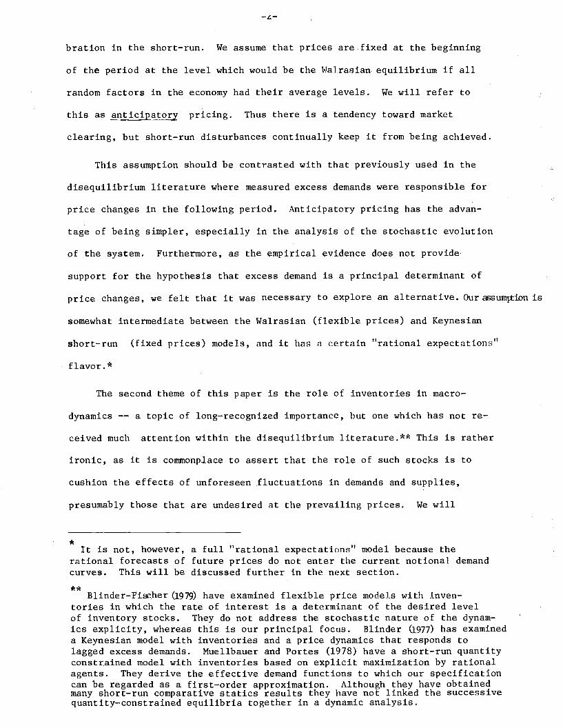
bration in the short-run. We assume that prices are.fixed at the beginning

of the period' at the level which would be the Halrasian· equilibrium if all

random factors in the economy had their average levels. We will refer to

this as anticipatory pricing. Thus there is a tendency toward market

clearing, but short-run disturbances continually keep it from being achieved.

This assumption should be contrasted with that previously used in the

disequilibrium literature where measured excess demands were responsible for

price changes in the following period. Anticipatory pricing has the advan-

tage of being simpler, especially in the analysis of the stochastic evolution

of the system. Furthermore, as the empirical evidence does not provide'

support for the hypothesis that excess demand is a principal determinant of

price changes, we felt that it was necessary to explore an alternative. Our assumrt:ion is

somewhat intermediate between the Walrasian (flexible prices) and Keynesian

short-run (fixed prices) models, and it has n certain "rational expectations"

flavor.*

The second theme of this paper is the role of inventories in macro-

dynamics a topic of long-recognized importance, but one which has not re-

ceived much attention within the disequilibrium literature.** This is rather

ironic, as it is commonplace to assert that the role of such stocks is to

cushion the effects of unforeseen fluctuations in demands and supplies,

presumably those that are undesired at the prevailing prices. We will

* It is not, however, a full "rational expectations" model because therational forecasts of future prices do not enter the current notional demandcurves. This will be discussed further in the next section.

** Blinder-Fischer (1979) have examined flexible price models with inven­tories in which the rate of interest is a determinant of the desired levelof inventory stocks. They do not address the stochastic nature of the dynam­ics explicity, whereas this is our principal focus. Blinder (977) has examineda Keynesian model with inventories and a price dynamics that responds tolagged excess demands. Muellbauer and Partes (1978) have a short-run quantityconstrained model with inventories based on explicit maximization by rationalagents. They derive the effective demand functions to which our specificationcan be regarded as a first-order approximation. Although they have obtainedmany short-run comparative statics results they have not linked the successivequantity-constrained equilibria together in a dynamic analysis.

-3-

analyze how the level of inventories interacts with the level of prices

and wages, and how the spillover effects in a fixed-price equilibrium

produce certain testable characteristics in macro time series data.

We will argue that these can be used to discriminate between a model of the

type we study and the analagous flexible-price system.

In Section 1 we set out the basic model and discuss its assumptions.

Section 2 derives the short-run quantity-constrained equilibrium as it

depends on initial inventory stocks and on the random disturbances within

the period. Section 3 presents, for comparison purposes, the analagous

results under conditions of full price flexibility after these shocks

are realized.

Sections 4 and 5 are the heart of the paper. We first derive the

probabilistic nature of the equilibrium under a variety of stochastic

specifications. The probabilities of different types of quantity constrained

equilibria can be compared under these alternative hypotheses. Then, we

use these results to present the dynamics of inventory behavior and the

statistical relationships between real wages, inventories and employment.

We emphasize the possibility of using this type of analysis to test the

disequilibrium hypothesis with anticipatory pricing, against the market­

clearing assumptions.

Our theoretical model suggests several lines of empirical investigation.

In an appendix, we present some time series evidence on the relationships

between the important variables of our system. These are of a preliminary

nature and are not des1gned to test our view of the theory presented. They

are nevertheless suggestive particularly because of the unexpectedly large

effect of inventories on the real wage.

Rational a~entR should recognize t~e influence of firms' inventories ontheir future profit irtcome, but we have neglected that as well. In futurework we. will addr.'e§slsavings ~nd asset markets, uarticulaIly the relationb~t:WQ~h rt\~rley afU ;! c. -Hms t, ',ital as stores ot value, . n disequilibrium.

-4-

1. The Model

Basic Structure

The model to be described below has two stores of value, money and in-

ventories, which interact together with the flow demands and supplies on

the labor and output markets to determine a short-run equilibrium. Successive

short-run equilibria are linked together by the dynamics of inventory move-

ments and the prices and wages which result from them.

Before deriving the stochastic structure of this dynamic disequilibrium

process, we should discuss the nature of the model -- and especially the

central role to be played by inventories and the price formation mechanism.

Inventories are accumulated as the result of an excess of output over sales

*to consumers. It is assumed that such sales of output are entirely con-

sumed; the inventories are owned exclusively by firms. Similarly, money

balances are held only by households. They are used to finance purchases

of goods in excess of labor income. Both inventory levels and real money

balances are desired because they provide the individual decision makers

with flexibility in case they are unable to fully execute their desired trans-

actions. In the aggregate, therefore, we will assume a positive desired in-

ventory stock and that the level real balances enters the demand and supply

** ***function of households.

* Bl inder (1978) offers an extensive discussion of inventories as inputs, butfinally assumes that their role as residual output is dominant, as we do.

**It should be mentioned, or rather confessed, at the outset, thattl1is form-ulation does not treat the role of firms' profits and their imputation backto the household sector in a consistent fashion. Implicitly, any money balancesaccumulated by firms are immediately transferred back to the household sector,but these profits are not anticipated at all. Hnner competitive conditions -­that is with many households, each of whom treats profit income as independentof their own actions -- this formalization is consistent with a 100% profitstax and a monetary policy designed to keep the nominal stock of money constant.

***

-5-

Because firms wish·to maintain some inventories, part of planned pro­

duction may be intended for inventory accumulation. An increase in inven­

tory stocks is not, by itself, enough to indicate that fi rms could not sell

all they wanted to. The actual variation in these stocks is a composite of

the intended and unintended changes.

The price-setting process is conceptualized as follows: Time is measured

in discrete intervals. The level of inventories is known at the beginning of

each period. Further the expected values of demands and supplies of goods and labor

as functions of the nominal prices and the stocks of money and inventories

are known. These functions may differ from their expected values because

of unforeseeable, random events. Prices are set during the period at

the values that would clear the market if these expectations were all

realized. During the period they remain rigid, and it is this inflexibility

which is the source of the disequilibrium dynamics that we will be studying.

Obviously the extreme nature of this process is not to be justified

on the grounds that it precisely represents the workings of any economy.

Moreover, the length of the period affects the extent of the disequilibrium

generated by the temporarily frozen price levels in a serious way, and no

one choice can really be defended. Nevertheless we believe that the study

of this model can provide useful insights and that it can be viewed as an

approximation to an actual economy in which a variety of disequilibrium

adjustments are taking place simultaneously. After giving an algebraic

statement of the model, we will return to such a discussion.

-6-

Mathematical Specification

In order to make the model tractable we will impose a linear struc-

ture on the supply and demand functions. Following Barra - Grossman (1971)

and Malinvaud (1977) the amount by which an agent is constrained below his

desired level of purchase or sale in one market enters intb the determination

of his desired trade in the other market. These "spillover effects" are

also assumed to be linear. For the production sector we have

(1.1)

(1. 2)

where

sx

t= desired level of supply (i.e. of actual sales) to the

household sector

£d = desired level of labor demand·t

Pt,Wt

= logarithm of price level and wage rate, respectively

xt'£t actual, market-determined sales and empioyment

St = inventory stocks at the start of the period

s = desired level of inventory stocks in a steady-state

1 3E ,E = random errors

t t

all in period t.

One should note that if the firm is interested in maximizing the present

value of its profits, expressed in real terms in units of output, it follows

that

(1. 3)

and

(1. 4)

-7-

a = -a > 01 2

Yl = -Y 2 > 0

Suppose that the marginal product of labor is g > 0, and that it is

regarded as a constant over the range of variation we are considering. It

is natural to assume that if the sales are rationed by an additional unit,

sthat is if xt

< xt

and xt

decreases by one unit, then the decreased demand

for labor would be such as to decrease actual output by less than one

unit, the residual being used for inventory accumulation. Thus we have

(1. 5) o < c < llg

This can be derived from the second order conditions for the firm's problem.

Similarly an extra unit constraint on labor demand should be absorbed par-

tially by a reduction in inventory stocks and partially by a decrease in

the volume of goods offered for sale.

(1. 6) o < a < g •

Finally, an extra unit of inventory should result in a mixture of

sales increase and labor demand decrease. However, since the adjustment

made within one period is only partial,

(1. 7)

with

(1. 8)

a o - gyo < 1

-8-

(For a formal derivation of similar restrictions see Blinder and Fischer(l978».

For households we have the behavioral relations

(1. 9)

(1.10)

h Xd and nS h d d f d d ff fw ere ~ are t e eman or goo s an 0 er 0 labor services

t t

respectively.

The theory of household behavior differs from the theoryeor firma

because it is the households who hold money balances. Since we will treat

the case of a constant money stock throughout, nominal prices and price

expectations are sufficient to specify the level of real balances. Because

we take the view that the unit of time is rather short compared with the

planning horizon of the household, the principal determinant of the house-

holds' demand for real balances is its expectation of future prices and

wages. It will be shown below that prices in any period depend solely on the

predetermined inventory level. Moreover, because inventories will follow

astationary Markov process, in the long run the average level of prices

and wages is known. Under these conditions the price and wage expectations

relevant to demands at any moment in time can, to a first approximation, be

regarded as exogenous and fixed. Thus (1.9) and (1.10) include prices

and wages because of their short run effects, but need include neither

*expectations nor money balances explicitly.

The standard theory of consumer behavior over time would give us a

zero degree homogeneity of market behavior in prices and wages for the

* Since (p , w , s ) will follow a Markov process, future values of (p , w )t t t ..t.. tcan be forecasted from present ones. Thus priceR and wages enter (1..'1) and

(1.10) in their role as predictors as well as through intertemporal substi­tution effects.

-~-

current and all future periods. If nominal prices in the short run were to

increase, the constancy of long-run expectations would imply a negative

"real-balance effect".

Assuming that consumption and leisure are all normal goods, we have

. that

(1.11)

(1.12)

Further,

(1.13)

follows from standard considerations of demand theory. The signs and

magnitudes of 01 and 02 cannot be derived from such considerations; but we will

sometimes assume that they are both relatively small, as empirical evidence suggests.

Using these conditions to simplify the system we have that

(1.14)

(+) (+) (+)

(1.15)

(- ) (+) (+)

(1.16)

(- ) (+) (+)

(1.17)

(- ) (+) (+)

where the signs indicate the assumptions being made on the indicated

parameter.

Finally, to close the model, we make the standard disequilibrium

theoretic assumption that actual quantities are determined by the "short-

-10-

side" of each market:

(1.18)d xd )xt

.. min (xt ' t

(1.19) R, = min (R,d 1s

)t t' t

While these quantity adjustment rules can be criticized on several grounds,

they have the great advantage of providing analytical tractibility. They

also lead to a theory that can, in principal, be tested against a corre-

sponding equilibrium theory.

The basic assumption of our model is that Pt and wt

are set in advance

at the level that would clear the market if there were zero errors in each

of the behavioral equations. Defining these levels as p~, w~ we have,

(1. 20)

(1. 21)

yielding

(1. 22) p*t

(1. 23)

Let

(1.24)

Prices are fixed at these

the values of random variables

levels at the beginning of the period, then

1 2 3 4(£ , £ , £ , € ) are realized so that (p*, w*)

t t t t t t

is not a Walrasian equilibrium price system in Reneral. We study a fixed-

-11-

,price equilibrium in which the quantities x and £ serve as the equilibratingt t

variables. That is, one can imagine sales and employment varying until, at

their equilibrium levels, the system of equations given by (1.14) - (1.19)

is satisfied.

Discussion of the Model

Although there is no firm microeconomic foundation for our assumption

that prices are fixed at their anticipated Wa1rasian levels, and are then

frozen there for the ensuing period, we had several reasons for adopting

such a formulation. It is clear that in any macroeconomic model that deals

with sufficiently short time periods, neither the assumption of perfect

price flexibility nor the assumption of quantity flexibility would be

rea~onable. The world is in continual disequilibrium to a much greater

extent then either pure formalization admits. In this paper we will

emphasize quantities as the equilibrating vRr:l.ables. while recognizi.ng

that this is but one extreme among a continuum of possibilities. In any

context where one adopts either the strict price-flexibility or quantity-

flexibility paradigms, the length of the period in question makes a big

difference as to whether the model does or does not approximate the reality.

Our choice of the price level at the anticipated Wa1rasian equilibrium

should be compared with several other possibilities. Most of the literature

*on disequilibrium macroeconomics has assumed that prices adjust from their

lagged values according to the lagged value of excess demand. In our model,

* In the econometrics literature, both adjustment of prices to past excessdemands and partial adjustment to current excess demands have been used (seefor example Fair and Jaffee [1974], Laffont and Garcia [1977]. In theeconomic theory literature adjustment to past excess demands has been therule (see Honkapohja [1979], Laroque (forthcoming».

//

~12-

one of the impacts of previous disequilibria is to alter the level of

stocks. Therefore prices in our model will be higher after a period of

excess demand for goods, as in these systems. The analogous property

does not apply to the wage rate, as labor services are not durable, nor

is there explicitly intertemporal substitution of labor for leisure over

individuals' lifetimes.

These two price adjustment hypotheses are hard to compare on empirical

grounds. One reason why prices are likely to appear responsive to lagged

excess demands is the auto correlation of errors. However, such an obser-

vat ion would not contrad~ct the basic motivation for having an anticipatory

pricing process. For contractual reasons, or because of the difficulty of

monitoring and responding to the current state of disequilibrium t the firms

and workers might try to use pricing rules designed to approximate an

*efficient market-clearing system.

In planned economies there is some evidence that prices are set so

as to approximate equilibria that are forecasted. This may provide a justi-

fication of our anticipatory pricing assumption in modelling such systems.

* To take one alternative, we might suppose that prices are set at themathematical expectation of the ex post equilibrium. The difficultywith this assumption is that the bias of these prices away from ~* , w*)

. t tdepends upon the distribution of the disturbances €. Therefore a complicatedpair of non-linear equations would have to be sOlvea to find the prices andwages, in contrast to the simple system (1.20) .- (1.21).

Another price-setting mechanism is that prices are only incompletely flexiblewithin the period. They end up somewhere between their lagged values and thelocation of the market-clearing equilibrium. This amounts to an adjustmentin response to current, rather than lagged, excess demands. This hypothesisis attractive in that the length of the period can be reflected in the speci­fication of the adjustment speed. Unfortunately we were unable to obtaintractable dynamic results.

-13-

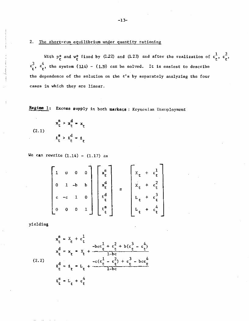
2. The short-run equilibr~um under quan~ity rationi~

1 2With p~ and w~ fixed by (122) and (123) and after the realization of E

t, E

t,

3 4Et , Et , the system (114) - (l.B) can be solved. It is easiest to describe

the dependence of the solution on the E'S by separately analyzing the four

cases in which they are linear.

!egime 1: Excess supply in both markets: Keynesian Uncnployment

8 dx t > x = xtt(2.1)

tS

> td = tt t t

We can rewrite (1.14) - (1.17) as

1 0 0S 1

U x Xt + Ett

0 I -b b d + 2xt Xt

Et=

I 0 t d + 3c -c t L

tE

t

0 0 0 1 t SL + 4

t t Et

yielding

8 X + 1x • e:

tt t 123 e: 4)d -bee: + e: + b(e: -

= ~+ t t t tx

t = xt I-be

(2.2) 1 2 3 4

t d -e(e: - e: ) + e: - beE= t = L + t t t t

t t t I-be

t S = L + 4t t

e:t

-14-

Regime 2: Excess supply on the good market and excess demand on the labor

market: Under Consumption

(2.3)

s dx > x· ... xt t t

R,d > 1s .. R.tt t

The structural equations are

1 0s .. + 1

a -a xt XtE: t

0 1 0 0d 2

xt Xt + E: t::

1 0 R.d + 3

c -c LtE:

tt

0 0 0 1 1s +4

Lt E: tt L

yielding

1 2 3 4E: - ac E:

t+ a(-E: t + E:

t)

s ... X + txt t 1 - ac

d"" X +

2xt.. x E: tt t

(2.4) 1 2 3 4

R.d ..

-c(E: - E: ) + E:t - ac E: tL +

t tt t 1 - ac

1s .. L "" B +4

t t tE: t

Re.s.ime 3: Excess demand in both markets: Repressed inflation

d sxt

> x "" xt t

(2.5)

R.d

> 1s .. R.tt t

-15-

The structural equations are:

sXt + 1

1 0 a -a xt £t

0d

Xt20 1 0 xt + £t

-Rod - 3

0 0 1 0 t tt + £t

0 1 t S + 4-d d t L t £t

yielding

1 2 3 4£t - ad £t + a(-£t + £t)

1 - ad

)2.0

t d.. L' + 3

t t £t

1 2- ad 3 + 4d(£ - £t) £t

tS

.. tt .. \: + t £tt 1 .,. ad

Regime 4: Excess demand on the good market and excess supply on the labor

market: Classical Unemployment

(2.7)

we have

-16-

1 0 0 0s

Xt+ 1x

t Et

0 1 -b b d 2x Xt + Ett =

0 0 1 0 R,d 3t L t + Et

-d d 0 1 R,s 4t L t + Et

yielding

s 1xt

.. x .. X + Et t t

-bd 123 4d

Et + Et

+ b(Et - E )

Xt + tx ..1 - bdt

(2.8),td.R, .. L + 3

t t t Et

1 2 3 4d(E t - e: ) - bd Et + EtR,s .. L t +t

t 1 - bd

Within each regime we can study the stability of the natural quantity

adjustment processes

hId xs ) yt)x

t= (min(x

tt

t(2.9)

hZd R,s) - R, )R,t = (min(R,e t t

where hI and hZ are sign-preserving functions. It follows from an examination

of the linear systems (Z.2)t (2.4)t (Z.6) and (2.8), that this dynamic

adjustment process would be locally stable provided that,

1 - be > 0

1 - ac > 0(2.10)"

I - ad > a

1 - bd > a

-17-

For example, suppose that an equilibrium in Regime 1 were disturbed by a

small upward perturbation in sales of ~Xt. This would produce. a lower level

of constraint in the supply of goods and hence an increase of c~x in thet

demand for labor. The change would give rise ·to more demand for goods by

bc~xt. Summing up the induced increase in demands] stability requires 1 - bc > O.

Now, when we consider the entire equation system in which these

regimes are juxtaposed it has been shown by Gourieroux, Laffont and

Monfort [1978] that the existence and uniqueness of the quantity-constrained

solution is implied when these local stability properties hold within each regime.

Let us compute the constraints on the ~'s such that the realized values

of demands and supplies satisfy the definition of each of the regimes. For

example, assuming that we are in Regime

(2.2) and if they are to satisfy (2.1) we must have that

1 2 b(~3 40~ - ~ ~ ) >

t t t t(2.11)

1 2 3 ~4) > 0c(~ - ~ ) - (~ -t t t t

and conversely, if (2.1]) is satisfied, then the solution to (2.2) will lie in

Regime 1. Pursuing this method for the other regimes we find that they are

realized if the £'s lie in the following region~;

Regine 24e: ) > 0t

(2.12)

Regime 3

(2.13)

-18-

Regime 41 2 3 e: 4)(e: - e:

t) - b(e: <0t t t

(2.14)d(e:1 2 3 4- e: ) - (e: - e: ) > 0

t t t t

A direct comparison of (2.11) - (2.14) reveals that, under the conditions

( ....\ h i f i i f 1 f 11 (1. 2 3 1+)2.1~, t ese reg ons arm a part t on 0 tle space 0 a £t' £t' £t' £t

vectors.

Let

1 1 2v = £ - £

t t t

(2.15)2 3 4

v = £ - £t t t

One can see directly that the four different regimes can be represented

in the (vI 2)t' v t

space (see Figure I,next page).

-19-

:',

.~... '

;.;,r~':··,....C~~~b)

.,(1"";,; .,,:: .,1'

.. ,,1;;'

~W£~f\bd~;

(R~a~lt)

In this fi gure we considermotivated i the casen the a > b,

next section.

c > d which will be

-20-

3. Short-run equilibria with~~ice flexibility

For future reference, it is useful at this point to derive the

prices, wages and equilibrium quantities that would arise if prices and

wages were to adjust so as to clear both markets after the realization of

the disturbances. Setting (1.14) equal to (1.15), (1.16) equal to (1.17)

and ignoring all the terms involving sp,illover effects we can derive the

following expression for the equilibrium real wage:

(3.1) ~ • (w~ - p~)= [Yo (81 + 82) + a O (01 + 02)] (St - s)2 1

+ (61 + S2) vt

- (01 + 02) vt

where ~ is given by (1.24). Equilibrium employment, and hence output, are

given by

(3.2)

The stability condition on the Walrasian price adjustment process

where wages respond to excess demand in the labor market and prices to

excess demand in the goods market implies that f.. < O. These stability con-

ditions will be satisfied whenever 01 and 02 are relatively small (see

the right hand side of (1.24». The comparative statics of the equilibrium

model with respect to inventories and shocks can be derived in a straight-

forward way. It may be seen that the real wage responds negatively to

initial inventories, positively to shocks that increase the excess demand

for labor, and positively to shocks that increase the excess demand for

goods. These comparative statics are in accordance with one's intuition

that initial inventories are a substitute for labor inputs in the short-run

production process.

-21-

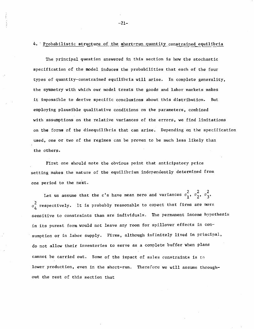
4. ' Probabilistic structure of the short-run quantity'- constrained equilibria

The principal question answered in this section is how the stochastic

specification of the model induces the probabilities that each of the four

types of quantity-constrained equilibria will arise. In complete generality,

the symmetry with which our model treats the goods and labor markets makes

it impossible to derive specific conclusions about this distribution. But

employing plausible qualitative conditions on the parameters, combined

with assumptions on the relative variances of the errors, we find limitations

on the forms of the disequilibria that can arise. Depending on the specification

used, one or two of the regimes can be proven to be much less likely than

the others.

First one should note the obvious point that anticipatory price

setting makes the nature of the equilibrium independently determined from

one period to the next.

222Let us assume that the E'S have mean zero and variances 01' 02' 03'

o~ respectively. It is probably reasonable to expect that firms are more

sensitive to constraints than are individuals. The permanent income hypothesis

in its purest form would not leave any room for spillover effects in con-

sumption or in labor supply. Firms, although infinitely 11ved in principal,

do not allow their inventories to serve as a complete buffer when plans

cannot be carried out. Some of the impact of sales constraints is to

lower production, even in the short-run. Therefore we will assume through-

out the rest of this section that

-22-

a > b(4.1)

c > d •

To derive the probabilities of the four regimes we use the inequality

constraints defining them (2.LI) ­

1written entirely in terms of vt

=

Independent Shocks

(2.14) •

1 . 2E: - E:

t t

These

2and v

t

constraints

3 4E: - E:t t·

can be

The first specification of the errors that we will consider is the

case in which they are independently distributed.

It is natural then to define

2 2 2° == °1 + °2v1

(4.2)2 2 2

° • °3 + °4v 2

I Li l-l / 2

Pr[Regime i] == --:::"21T---

If in addition we postulate normality, then

5fo 0

with

r •1

-23-

1: • (2 + 22 d02 +002

1o a 03 v

lv2 vl v2

d02

+ 402 d20

2 +02vl v2 vl v2

I: 4 •2 + b

20

2 2 20 -do - bovl v2 vl v2

2 2 d202 +02

-do - bovl v2 vl v2

The probabilities of the different regimes can be ranked according

to the Correlation coefficients, Pi between ~ and ~2 as specified by the

matrices 1: i.

P2 =

d 2 + 2 2o a 0P = v l v 23

2PI ~ I - (b - lie)

2P3 W 1 - (a - lid)

-24-

The highest probabilities are associated with the Keynesian unemp1oy-

ment (Regime 1) and repressed inflation (Regime 3) modes, where the corre-

lations are positive. An intuition for this result can be derived from

the observation that when errors occur one at a time only Regime I and 3

are possible. This point is due to the fact that the first effect of a

shock is to constrain one agent (firms or consumers) in one market and by

the spillover effect the other agent in the other market. The stability

conditions imply that one remains then in a regime where both agents are

constrained, i.e. either Keynesian unemployment or repressed inflation.

The comparison between Regimes I and 3 and between Regimes 2 and 4 is

difficult and depends on the variances and on the spillover coefficients.

One possibility to obtain further results can be obtained if we are willing

to make the assumption that shocks originating on the consumers' side of

both markets are small compared to producers shocks.* This can be de­

22·scribed by letting a /a be small. Under these conditions PI and P3 can

v2 vIbe approximated as

2av2-ravI

2av2

-r-avI

Regime 1 will be more likely than Regime 3 if

2 2(a - lid) > (b - lie)

* This is the implicit assumption in much of Keynes and is made explicit inthe work of Malinvaud.

-25-

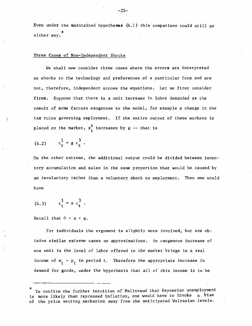
Even under the maintained hypotheses (4.1) this comparison could still go

*either way.

Three Cases of Non-Independent Shocks

We shall now consider three cases where the errors are interpreted

as shocks to the technology and preferences of a particular form and are

not, therefore, independent across the equations. Let us first consider

firms. Suppose that there is a unit increase in labor demanded as the

result of some factors exogenous to the model, for example a change in the

tax rules governing employment. If the entire output of these workers is

splaced on the market, x increases by g -- that ist

(4.2)

On the other extreme, the additional output could be divided between inven-

tory accumulation and sales in the same proportion that would be caused by

an involuntary rather than a voluntary shock to employment. Then one \JOuld

have

(4.3)

Recall that 0 < a < g.

For individuals the argument is slightly more involved, but one ob-

tains similar extreme cases as approximations. An exogenous increase of

one unit in the level of labor offered to the market brings in a real

income of wt - Pt in period t. Therefore the appropriate increase in

demand for goods, under the hypothesis that all of this income is to be

* To confirm the further intuition of Malinvaud that Keynesian unemploymentis more likely than repressed inflation, one would have to invoke a biasof the price setting mechanism away from the anticipated Walrasian levels.

spent, is wt

- pt'

...26~

Under this assumption, the relationship between the

4 2shocks to labor supply, € , and goods demand, e , depends on the pricest t

prevailing in that period. This would make the analysis of the quantity-

constrained equilibrium virtually as complex as the system with independent

errors. It is more tractable if we take the approximation that wt

- Pt is,

in the long-run, equal to the real marginal product of labor g. This would

give us

(4.4)

which is analagous to (4.2). Alternatively, we can suppose that the extra

earnings are divided between spending on goods and accumulation of money

balances in the same proportion that the individual allocates his constrained

labor income. Since one unit less of labor supply causes goods demand to

drop by b, we obtain

(4.5)2

et

It is possible to examine each of the four possible combinations of

these assumptions (4.2) or (4.3), together with either (4.4) or (4.5). To

obtain the flavor of the analysis, however, we report on only three of these

cases. We will see that the results are rather sensitive to this specification.

(4.2) and (4.5) : (Firms'shocks affect flows only, individuals' shocks affectdemands for money and goods)

The regimes are then defined by

Regime 1

Regime 2

(g - b) e 3 > 0t

(eg - 1) €~ + (1 _ be) 4 > 0 '€t

3 4(eg-l)€t + (l-eb)e t < 0

Regime 3

Regime 4

Then

p •1

(4.6)

-27-

3 4(g-ah: + (a-b) E <-0t t

(dg-l)e:~ + U-bd)e:;' < 0

3(g-b)E < 0t

3 4(dg-l)Et

+ (l-bd)Et

> 0

2 2_ (g-a) (cg-l)03 + (a-b)(1-cb)04

2 2 2 2 2 2([(g-a) 03 + (a-b) 04][(cg-l) 03 +

·22= (g-a) (dg-l)o3 + (a-b) (1-bd)04

P322 22 22 22 ~

([(g-a) 03 + (a-b) 04][(dg-l) 03 + (I-bd) 04])

p = _ (dg-l)034 -----------

2 2 2 2 ~«dg-I) 03 + (l-bd) 04)

Uoing (4.1) we find that PI < 0: 04 > 0, (JZ ann (>3 being aMbipuous. If

the shocks on the consumer side are also smaller than on the producer side

we have in general Pz > 0 P3

< 0, thus ranking Regimes 2 and 4, under

consumption and classical unemployment, "Tit;) the highest probability. If

the shocks on the consumer side are greater (because of shocks in demand)

we get Pz < 0 and P3

> O. Repressed inflation and classical unemployment

become the most likely regimes.

-28-

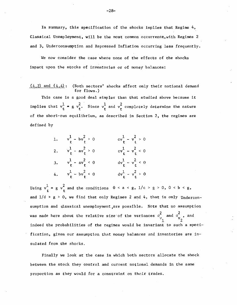
In summary, this specification of the shocks implies that Regime 4,

Classical Unemployment, will be the most common occurrenc~,with Regimes 2

and 3, Underconsumption and Repressed Inflation occurring less frequently.

We now consider the case where none of the effects of the shocks

impact upon the stocks of inventories or of money balances:

(4.2) and (4.4): (Both sectors' shocks affect only their notional demandfor flows.)

This case is a good deal simpler than that studied above because it

implies that v~ = g v~. Since v~ and v~ completely determine the nature

of the short-run equilibrium, as described in Section 2, the regimes are

defined by

1 2v - av > 0

t t

I 2v - av < 0

t t

1.

2.

3.

4.

1v

t

1v

t

I 2cv - v > 0

t t

1 2cv - v < 0

t t

dvl _ v2< 0

t t

dvl _ v2> 0

t t

1 2Using v = g v and the conditions 0 < a < g, llc > g > 0, 0 < b < g,t t

and lid> g > 0, we find that only Regimes 2 and 4, that is only Undercon-

sumption and classical unemployment ,are possible. Note that no assumption

2 2was made here about the relative size·of the variances 0 and 0 , and

vI v2indeed the probabilities of the regimes would be invariant to such a speci-

fication, given our assumption that money balances and inventories are in-

sulated from the shocks.

Finally we look at the case in which both sectors allocate the shock

between the stock they control and current notional demands in the same

proportion as they would for a constraint on their trades.

-29-

(4. i and (4.5): (Both sectors' shocks affect notional demands for flowsand stocks.)

Substituting into the basic definitions of the regimes we obtain

3 4their dependence on e: t and e: t in this case:

1.

2.

3.

4.

3(a-b)e: > 0t

3 4-(l-ac)e: + (l-bc)e: > 0t t

4(a-b)e: > 0

t3 4

0-(l-ac)e: + (l-bc)E: <t t

4(a-b)E < 0t

3 4-(l-ad)E + (l-bd)e: < at t

3(a-b)e: < a

t3 4

- (l-ad)E + (l-bd)E: > a .t t

2 2If we assume that a /a

v2 vI

ishingly small probability and

3e: > 0, the

t

is small we find that Regime 1 has a van-

3that Regime 4 will occur whenever E: < O. lHth

t4

sign of E: determines whether we are in Regime 2 or 3. There-

fore the appropriate probabilities of Regimes 2, 3, and 4 are 1/4, 1/4,

and 1/2 respectively.

2 2The. case of a /a small, which admittedly has little support in the

VI v2literature, would yield asymptotically the probabilities (1/4, 0, 1/2, 1/4)

for the four regimes respectively. Combining these results we see that

Regimes 3 and 4 are going to be more likely than Regimes 1 and 2, whatever

the error structure is. The goods market is systematically more likely to

be in excess supply than in excess demand!

-30-

We can see t therefore t that the nature of the shocks is an important

determinant of the probability of reaching any of the regimes. If direct

evidence were available as to the nature of the binding quantity constraints

*at different points in time, indirect evidence would be available as to the

relative magnitude of the shocks.

* For example, suitable unemployment/vacancy data would be relevant tothe labor market. Evidence in the goods market is harder to ascertainsince intended inventory movements may be confounded with flow disequilibrium.

-31-

5. Dynamic Behavior of Quantity-Constrained E~ui1ibrium Process

In this section we will utilize the stochastic structure derived

above to study the dynamics of inventories, employment, output, the real

wage and correlations among them. We will compare the results of the

disequilibrium model to those arising from a system where prices are

flexible ~fter the realization of the shocks, as described in Section 3.

In particular we will ask whether or not these systems are "observationally

equivalent", and we will suggest methods for testing one of these hy-

potheses against the other.

The dynamics of inven~orie~

In this model inventories are entirely composed of unsold stocks of

final goods. Because there is no depreciation, the change in stocks is

simply the difference between production and sales. The evolution of in-

ventories is described by

(5.1)

Equation (5.1) is a stochastic difference equation because it and xt

are

random variables that depend on the underlying SIS, and on the current value

of St. Recognizing this dependence explicitly, we obtain a relation that

is piecewise linear in the £ •t

-32-

(5.2) gL -x +t t

2 4-e + ge

t t

I 2 3 4e (gd-l)+e d(a-g)+e a(l-gd)+e (g-a) ,

t t t· t

I 3-e + ge

t t

Regime I

Regime 2

Regime 3

Regime If

iLet ~ (e

t) denote the linear form in the £ associated with regime i,

in equations (5.2), i=I,2,3,4.Consider the anticipated change in inventory

stocks, that is, the change that would happen if all the e's were zero and

prices were set as we have postulated.

Let un define the coefficient on the right hand aide to be KO' a function

only of the parameters of the system. KO is the effect on the anticipated

change in inventories due to one unit of additional initial stocks. When

oI and O2

are small, it can be verified that 1 > KO

> 0 and hence that the

process is stable •

. We can express the dynamics of inventories in a succint way by de­

ifining the function He

t) to have the value of ep (e

t) whenever e

tlies in

regime i. Thus ~(€t) is defined over the whole range of et

. In this notation

(5.4)

or·

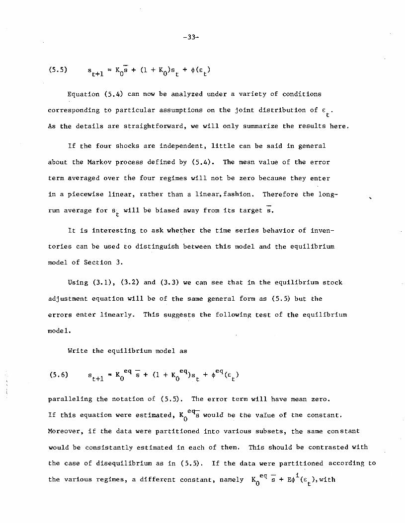
-33-

(5.5)

Equation (5.4) can now be analyzed under a variety of conditions

corresponding to particular assumptions on the joint distribution of £t

As the details are straightforward, we will only summarize the results here.

If the four shocks are independent, little can be said in general

about the Markov process defined by (5.4). The mean value of the error

term averaged over the four regimes will not be zero because they enter

in a piecewise linear, rather than a linear, fashion. Therefore the long-

run average for St will be biased away from its target s.

It is interesting to ask whether the time series behavior of inven-

tories can be used to distinguish between this model and the equilibrium

model of Section 3.

Using (3.1), (3.2) and (3.3) we can see that in the equilibrium stock

adjustment equation will be of the same general form as (5.5) but the

errors enter linearly. This suggests the following test of the equilibrium

model.

Write the equilibrium model as

"

(5.6)

paralleling the notation of (5.5). The error term will have mean zero.

eq-If this equation were estimated, KO

s would be the value of the constant.

Moreover, if the data were partitioned into various subsets, the same constant

would be consistantly estimated in each of them. This should be contrasted with

the case of disequilibrium as in (5.5). If the data were partitioned according to

th i i diff 1 Koeq -s + E~i( ) i he var ous reg mes, a ere.nt constant, name y ~ £t ,w t

..,.

-34-

the expectation conditioned on regime i~ would be observed in each regime.

Of course it is not obvious at all which regime is operative at which

point. Unlike previous work in disequilibrium econometrics~ the direction

of the price change in our model does not indicate anything about the

effective quantity constraints. Therefore the brute force procedure would

be to estimate the disequilibrium system by maximum likelihood methods

Tseparately for each of the 4 partitions of the T data points~ allowing

a different constant in each regime~ and·then to perform a likelihood

ratio test of the overall maximum likelihood among these reg.rcssions

against the equation estimated with a single constant.

Of course if T is fairly large this method becomes impractical. Some

economies of computation are possible~ however~ under more restrictive

hypotheses about the joint distribution of the components of £ •t

With the assumption that shocks do not impinge upon the notional in-

ventory~ but that individuals divide shocks between money balances and flow

demands) (4.2) and (4.5), we can derive from (5.2)

2 34E~ (£ ) = 0, E~ (£ ) < 0 and E~ (£ ) = 0 (indeed

t t t

> 0,

These quali-

tative constraints can be used to check the maximum likelihood estimations of

the four regimes: the estimated constants in Regime 1 exceed those of Regimes

2 and 4 which in turn exceed that in Regime 3. Moreover these constraints

can provide an algorithm for partitioning the data, if (4.2) and (4.5)

are adopted as maintained hypotheses. For example, if a~ is thought to

2dominate 04' we know from (4.6) that Regimes 2 and 4 become far more likely

than 1 and 3. We might therefore begin by running the unconstrained regression

(5.5)~ ignoring the biased error term, and then assign that half of the data

'1cwith the largest residuals to Regime 4 and the others to Regime 2.

* This method is reminiscent of the Fair - Jaffee (1972) procedure.

-35-

Another case of interest, paralleling the treatment of the last section,

occurs where the shocks affect current notional demands and desired stocks

in the same proportion as would quantity constraints: (/•• 3) and (4.5).

We have from (5.2) that

(5.7)

Recalling the results on the probability distribution over these

2 2regimes when 0 /0 is small we know that Regime I is not possible, and

v2 vI

3 4Regimes 2, 3, and 4 occur approximately whenever £ > ° and £ > 0,

343e:> ° and e: < 0, and e: < ° respectively. From (5.7) we see that the biases

induced in the constants in Regimes 2 and 3 will be small, since E£4 1e:4

> °31 3is small compared to Ee: e: < 0. Thus an~proximate test of the disequilibrium

model under the maintained hypotheses (4.3), (4.5), is to segregate the data

into two subsets, presumably those in or out of Regime 4, and test for the

inequality of the constants in these separate regressions. (Of course this

will be a weaker test than the full maximum likelihood procedure, but the

computational advantages may be significant.)

Other combinations .of (4.2) (4.3) and (4.4) (4.5) can be studied with

similar results.

Correlation between real wag~~__an~~qy~~tories

In the disequilibrium model we have studied, the anticipatory nature of

the price adjustment process makes the real wage a function of inventories

-36-

alone. Therefore, in the absence of observational errors, a perfect

(negative) correlation between them would be observed.

The equilibrium model's real wage is given by (3.1). It is easy to

show that the coefficient of (s - s) is the same in this equation as it ist

in the disequilibrium theory. The two dHfer only in the presence of the

error term. Because of observational errors, however, we cannot discriminate

between them.

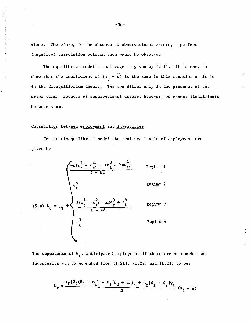
Correlation between employment and_j~~~ntories

In the disequilibrium model the realized levels of employment are

given by

1 - bc

(5.8) R,t

1 2 3 4d ( e: t - e: t) - ade: t + e: t

1 - ad

Regime 1

Regime 2

Regime 3

Regime 4

The dependence of L t , anticipated employment if there are no shocks, on

inventories can be computed from (1.21), (1.22) and (1.23) to be:

-37-

In the equilibrium model employment is given by (3.2). Note that the

systematic dependence of employment on inventories is the same under either

theory.

As in the case of the autocorrelation of the inventory series, the

difference lies in the stochastic structure. Different constant terms in

the regressions within each regime would provide evidence for the dis-

equilibrium hypothesis.

We will not elaborate upon the possibilities under all the stochastic

specifications treated previously. It is useful, however, to examine one of

them again because it indicates how a combination of evidence on inventories

and employment can help identify regimes and provide a sharper discrimination

between these theories.

Consider the case of (4.3) and (4.5), where disturbances impinge upon

notional demand for stocks in both sectors. The relations (5.8) become:

(l-ac) 3I-be Et

4E

t(5.9) ~ B

t+

t4

Et

3E

t

Regime 1

Regime 2

Regime 3

Regime 4

equation (5.7).

Compare these errors to the analagous terms in the inventory dynamics

2 2When d fa is small, the sign of the errors in each ofVz vI

the three possible regimes is precisely the same in (5.9) as it is in (5.7).

Therefore, if we identify a particular partition of the data points for one

equation, then under the maintained hypotheses about the errors, the constants

-38

estimated by maximum likelihood from the other equation should stand in the same

relationship across the regimes when the data are partitioned the same way.

2 2Indeed a further check is possible, using the fact that a fa isv2 vI

small. We can neglect the difference between the constants estimated in

Regimes 2 and 3 compared with their relation to that in Regime 4. From

(5.9) and (5.7) we can see that the difference between Regime 4 and the

other two in the employment regressions is E£~I£~ < 0, and in the inven­

tory autoregression it is (g~a) E£3 1£3 < O. We can infer that the cross-t t

equation difference in the constants in the inventory autoregression

should be less than g times the bias in the employment regressions, because

a > O. (The productivity of labor, g, can be estimated as the average real

wage, so this procedure is well-defined.)

Correlation between real wages and~loyment

Both the disequilibrium and equilibrium models predict a negative

correlation between real wages and employment when (01 + 02) is relatively

small. Tests based on the stochastic structure similar to those described

above can be constructed, but we believe that they will be harder to use.

There are difficulties in constructing a real wap,e series corrected for the

changing composition of the labor force and the problem of obtaining

wage rates when overtime and other considerations distort the relationship

between hours of employment and total earnings.

-39-

Appendix

We gather together a few regression results that are related to the

results of this paper. No attempt is made to give a detailed treatment of

problems in structural estimation of macroeconomic systems. These results

should be viewed merely as exploring some correlations in the data, and not

as necessarily confirming or disproving specific hypotheses.

Nevertheless we believe they are of interest. In particular they

point out the strong influence of inventories on the real wage.

The variables used are:

W, wage The real wage in the manufacturing sector. Computed as the

ratio"of hourly earnings to the implicit price deflator for

personal consumption expenditures.

H, hours The measure of total manufacturing employment. Computed as

the product of weekly hours for production workers with total

employment in the manufacturing sector.

INV, inventories Total inventories in the manufacturing sector.

IMP, import priceindex Index of unit-values of imported goods.

All data are seasonally adjusted.

We present three sets of regressions for monthly, quarterly and annual

data. In accordance with the theory, we treat as exogenous the initial level

of inventories.

In the monthly regressions we use the previous month's value. In

both quarterly and annual regressions we use the value associated with the

last month of the previous time period.

The wage, hours inventories and import prices are used in logarithms,

time is not used as a logarithm.

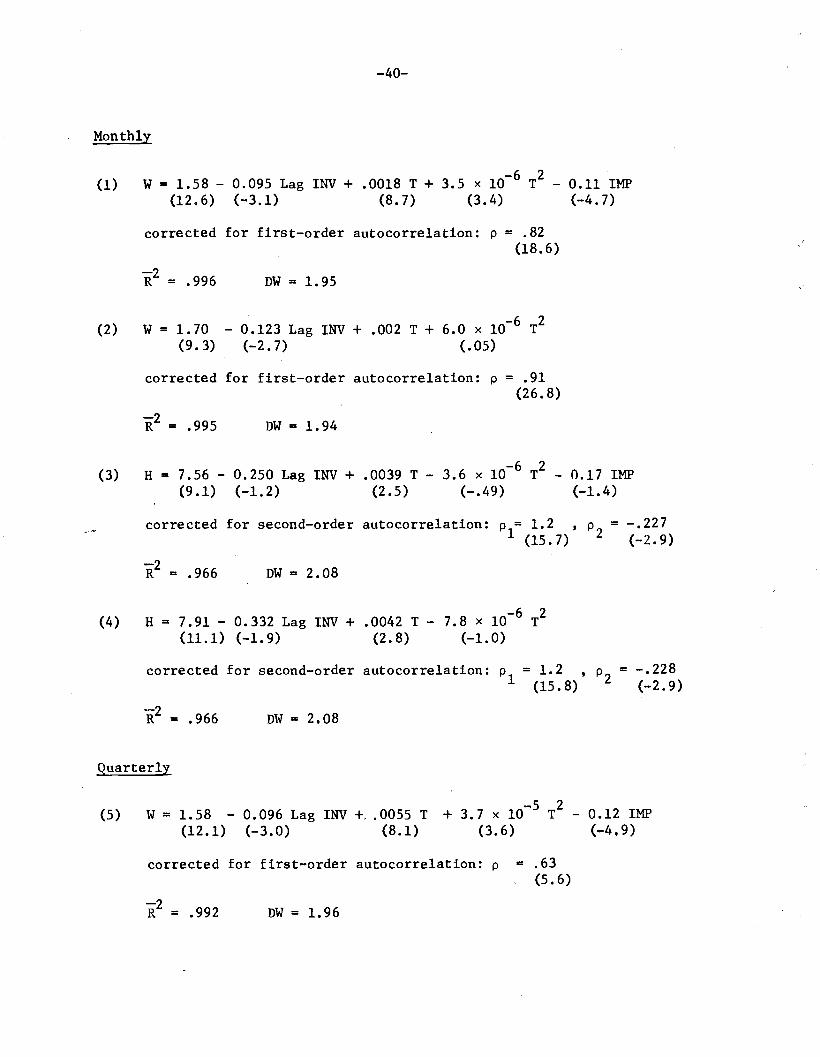
-40-

Monthly

(1)-6 2W= 1.58 - 0.095 Lag INV + .0018 T + 3.5 x 10 T - 0.11 IMP

(12.6) (-3.1) (8.7) (3.4) (-4.7)

corrected for first-order autocorrelation: p = .82(18.6)

DW ... 1.95

(2) W= 1.70 - 0.123 Lag INV + .002 T + 6.0 x 10-6 T2

(9.3) (-2.7) (.05)

corrected for first-order autocorrelation: p = .91(26.8)

-2R = .995 DW ... 1.94

(3) H = 7.56 - 0.250 Lag INV + .0039 T - 3.6 x 10-6 T2 - 0.17 IMP(9.1) (-1.2) (2.5) (-.49) (-1.4)

corrected for second-order autocorrelation: p = 1.2 ,p = -.2271 (15.7) 2 (-2.9)

DW ... 2.08

(4)-6 2H ... 7.91 - 0.332 Lag INV + .0042 T - 7.8 x 10 T

(11.1) (-1.9) (2.8) (-1.0)

corrected for second-order autocorrelation: p = 1.2 ,P2 = -.2281 (15.8) (-2.9)

-2R = .966 ml = 2.08

Quarterly

(5)-5 2W == 1.58 - 0.096 Lag INV +.. 0055 T + 3.7 x 10 T - 0.12 IMP

(12.1) (-3.0) (8.1) (3.6) (...4,9)

corrected for first-order autocorrelation: p = .63(5.6)

DW = 1.96

-41-

(6) W = 1.77 - 0.141 Lag INV + .0062 T + 3.5 x 10-6 T2

(9.3) (-3.0) (5.5) (.28)

corrected for first-order autocorrelation: P = .80(8.7)

-2R III .990 DW III 1.74

(7) H = 8.81 - 0.549 Lag INV + .0154 T - 3.9 x 10-5 T2 - 0.04 IMP(7.6) (-1.9) (2.5) (-.49) (-.Z6)

corrected for second-order autocorrelation: P1= 1.46 ,PZ = -0.54(10.9) (-4.3)

-2R .... 911 DW "" 2.05

(8) H "" 8.90 - 0.571 Lag INV + .0157 T - 5.0 x 10-5 T2

(8.5) (-2.2) (2.6) (-.69)

corrected for second-order autocorrelation: PI = 1.36 ,(11. 2)

P2 = -0.55(-4.4)

-2R = .913

Annual

DW = 2.04

(9) W • 1. 65(17.6)

- 0.116 Lag INV + .0228 T + .0006 TZ - 0.11 IMP(-5.0) (12.7) (3.0) (-4.9)

corrected for second-order autocorrelation: PI "" -0.48RZ .... 991 DW'" 2.43 (-1.4)

Pz = -0.46(-1. 3)

(10) W=1.71(8.0)

R2 = .970

- 0.129 Lag INV + .OZ5 T - 9.3 x 10-5 TZ

(-2.4) (5.7) (-.47)

DW = 1. 69

(11) W= 1.71 - 0.128 Lag INV + .025 T - 7.5 x 10-5 T2

(6.0) (-1. 8) (4.0) (-.33)

corrected for first-order autocorrelation: P = 0.10(0.2)

-2R a .966 DW"" 1.77

-42-

(12) W· 1.24 - 0.015 Lag INV + .0202 T - .0004 T2

(6.4) (-.32) (5.6) (-2.4)

corrected for second-order autocorrelation: P1= 0.33 , P2 = -0.81(1.3) (-4.5)

-2R = .982 DW = 2.25

(13) R .. 7.39(7.6)

'R2 = .045

- 0.201 Lag INV + .0343 T - .0004 T2 - 0.14 IMP

(-.84) (1.6) (-.27) (-.65)

DW = 1.17

(14) R = 8.54 - 0.494 Lag INV + .056 T - .0006 T2

- 0.10 IMP(5.8) (-1.4) (2.2) (-.34) (-.34)

Corrected for first-order autocorrelation: P = .62

(15)

-2R III .202

R'· 9.27(13.3)

DW ... 1.09

- 0.664 Lag INV + .0580 T + .0005 T2

- 0.13 IMP(-3.9) (2.7) (.28) (-.48)

corrected for second-order autocorrelation: PI

'R2= .615 DW = 1.61

= 1.18(4.6)

P2

= -0.77(-3.2)

(16) R = 8.72 - 0.537 Lag INV + .0632 T - .0010 T2

(8.6) (-2.2) (2.62) (-.69)

corrected for first-order autocorrelation: P = 0.65(2.1)

-2R = .280

(17) R = 9.45(15.8)

DW = 1.03

- 0.706 Lag INV + .0611 T - .0001 T2

(-4.8) (2.8) (-.11)

corrected for second-order autocorrelation: PI ... 1.23 ,P2= -0.77(5.1) (-3.7)

i 2 = .654 DW = 1.66

-43-

Summary of Results

The principal reason for performing three separate types of regressions

is that we do not know the timing of the anticipatory pricing and the shocks

which are supposed to be accomodated by disequilibrium quantity adjust­

ments. No attempt was made to search for regressions with more explanatory

power, but we do present two forms of the equations according to whether

the import price index variable is included. It was felt that this variable

is largely exogenous and that it exerts a strong influence on prices and

output quite independent of the inventory situation.

-44-

References

Barro, R.J. and H.I. Grossman [1971], "A General Disequilibrium Model of

Income and Employment," American Economic Review, vol. 71, 250-27l.

Benasay, J.P. [1975], "A Neo-Keynesian Disequilibrium in a Monetary Economy,"

Review_of !c!)fiom!c §!.udies, vol. 42 , 503-524.

Blinder, A. [10T1], "A DiUiculty uith Keynesian 1'1ooe18 of Ar,gregnte DeMand,"

in Natural Resources, Uncertainty and General Equi1ibri.um Systems,

essays in memory of Rafael Lusky, Academic Press, Inc.

Blinder, A. [1978], "Inventories in the Keynesian Macro Model," mimeographed,

Princeton University.·

Blinder, A.S. and S. Fischer [1979], "Inventories, Rational Expectations,

and the Business Cycle," National Bureau of Economic Research, Working

Paper No. 381.

Dr~ze, J.H. [1975], "Existence of an Exchange Equilibrium Under Price

Rigidities," IE.t~rnationa1 Economic Review, voL 16, 301-320.

fair, R. nnd D.t1. Jaffee [1972], "Methods of E1'lti:rnlltion for ~~nrkctD in

Disequilibrium," Econometric~, vol. 40, 497-514.

Fair R.C. and D.M. Jaffee [1976], "Methods of Estimation for Markets in, .

Disequilibrium: A Further Study," Econ0!1'etrica, vol.42, 177-190.

Gourieroux, C., J.J. Laffont and A. Monfort [1978], "Disequilibrium

Ecor..ometrics in Simultaneous Equation Systems," LM.S.S.S. report

Stanford University, Econometrica forthcoming.

Gourieroux, C., J.J. Laffont and A. Monfort [1979], "Coherency Conditions

in Simultaneous Linear Equation Models with Endogenous Switching

Regimes," N.B.E.R. Working Paper No. 343, forthcoming in Econometrica.

Eonl:npohln, S. [1979], "On the Dyn,mics 01: Discn'.d1ibrfum in n Macro Hodel

with Flexible Wages and Prices," in N. Aoki and A. Marzollo (eds.),

New Trends in Dynami~ System The~ ~nd Eco~omics, Academic Press.

-45-

Laffont, J.J. and R. Garcia [1974], "Disequilibrium Econometrics for

Business Loans," EC2nometrica, vo1.45, 1187-1204.

Ma1invaud, E. [1977], The ~eory of Unemployment ~ec£nsidered, Oxford:

Basil, Blackwell.

Muellbauer, J. and R. Portes [1978], "Macroeconomic Models with Quantity

Rationing;'Economi£ rourna1, vol. 88, 788-821.

-45~

Laffont, J.J. and R. Garcia [1974], "Disequilibrium Econometrics for

Business Loans," EC2nometrica, vo1.45, 1187-1204.

Ma1invaud, E. [1977], The ~eory of Unemployment ~considered, Oxford:

Basil, Blackwell.

Mue11bauer, J. and R. Portes [1978], "Macroeconomic Models with Quantity

Rationing:'Economic ~ourna1, vol. 88, 788-821.