discussion papers - diw.de

Deutsches Institut für Wirtschaftsforschung

www.diw.de

Burcu Erdogan

Berlin, April 2009

How Does European Integration Affect the European Stock Markets?

885

Discussion Papers

Opinions expressed in this paper are those of the author and do not necessarily reflect views of the institute. IMPRESSUM © DIW Berlin, 2009 DIW Berlin German Institute for Economic Research Mohrenstr. 58 10117 Berlin Tel. +49 (30) 897 89-0 Fax +49 (30) 897 89-200 http://www.diw.de ISSN print edition 1433-0210 ISSN electronic edition 1619-4535 Available for free downloading from the DIW Berlin website. Discussion Papers of DIW Berlin are indexed in RePEc and SSRN. Papers can be downloaded free of charge from the following websites: http://www.diw.de/english/products/publications/discussion_papers/27539.html http://ideas.repec.org/s/diw/diwwpp.html http://papers.ssrn.com/sol3/JELJOUR_Results.cfm?form_name=journalbrowse&journal_id=1079991

How Does European Integration

Affect

the European Stock Markets?

Burcu Erdogan∗

[email protected]

April 22, 2009

∗The author is a PhD candidate in Graduate Center of German Institute for EconomicResearch (DIW), Mohrenstr. 58, 10117 Berlin, tel.:+49-30-89789-285, fax:+49-30-89789-102.Acknowledgements: The research leading to these results has received funding fromthe European Community’s Seventh Framework Program (FP7/2007-2013) under grantagreement number 217266. The author would like to thank Kerstin Bernoth, KonstantinKholodilin, Ulrich Fritsche, Sebastian Weber, Guglielmo Maria Caporale, the discussantsof FINESS Steering Group Meeting; especially Sean Holly and Pal Gaspar; and FINESSInternational Scientific Conference; especially Timo Terasvirta and Eric Girardin for helpfuladvice and comments. Any errors are my own.

Abstract

This paper examines the integration of stock markets in Germany, France, Nether-

lands, Ireland and UK over January 1973-August 2008 at the aggregate market and

industry level considering the following industries: basic materials, consumer goods,

industrials, consumer services, health care and financials. The analysis is carried

out by using correlation analysis, β-convergence and σ-convergence methods. β-

convergence serves to measure the speed of convergence and σ-convergence serves

to measure the degree of financial integration. It might be expected a priori that

European stock markets have converged during the process of monetary, economic

and financial integration in Europe.

This study offers evidence for an increasing degree of integration both at the aggregate

level and also at the industry level, although some differences in the speed and degree

of convergence exist among stock markets. Surprisingly, there is an upswing of cross

sectional dispersion for health care industry, which is more prone to regional shocks.

The other industries show a significant σ-convergence. The average half-life of a

shock to convergence changes at a range from 5.75 days for aggregate market to

10.25 days for consumer goods.

Keywords: Financial integration, EU, stock markets, β-convergence, σ-convergence,

correlation analysis

JEL Classification: C22, G12, G15, F36

Table of Contents

1. Introduction 1

2. Methods to Measure Convergence 5

2.1. Correlations . . . . . . . . . . . . . . . . . . . . . . . . . . . . . . . . 5

2.2. β-Convergence . . . . . . . . . . . . . . . . . . . . . . . . . . . . . . . 5

2.3. σ-Convergence . . . . . . . . . . . . . . . . . . . . . . . . . . . . . . . 7

3. Empirical Analysis 8

3.1. Data . . . . . . . . . . . . . . . . . . . . . . . . . . . . . . . . . . . . 8

3.2. Correlations . . . . . . . . . . . . . . . . . . . . . . . . . . . . . . . . 9

3.3. β-Convergence . . . . . . . . . . . . . . . . . . . . . . . . . . . . . . . 10

3.4. σ-Convergence . . . . . . . . . . . . . . . . . . . . . . . . . . . . . . . 12

4. Conclusion 15

Bibliography 16

A. Appendix 19

ii

1. Introduction

In the last two decades, European financial markets have faced crucial structural and

institutional adjustments with the aim of accelerating the financial integration in

money, credit, bond, and equity markets. Integration of the financial markets adds

to the effective transmission of common monetary policy and to economic growth

by removing frictions and barriers to exchange and by allocating the capital more

effectively1. It is important to monitor the state of integration in various segments

of the market in order to identify areas where further initiatives are needed.

The focus of our paper is on equity market integration2. Integrated stock markets

generate better opportunities for international investors by eliminating country spe-

cific risks and let them diversify their portfolios across countries. A larger pool of

funds other than the limited local financing will be available for corporations. Inte-

grated stock markets decrease the cost of capital. Hence, the number of productive

investments increases, which flourishes the economic growth. In an economic en-

vironment where better risk-sharing opportunities exist, households will be able to

smooth their consumption more efficiently. Moreover, interdependent stock markets

are subject to spillovers resulting from shocks. Evaluating the dynamics of the equity

market integration is, therefore, important for monetary policy makers.

The main objective of this paper is to investigate the existence and the degree of

integration among stock markets in the five member states of the European Union

(EU); Germany, France, Netherlands, Ireland, United Kingdom (UK); at the country

as well as at the industry level. The following industries are under consideration:

basic materials, consumer goods, industrials, consumer services, health care and

financials.

1Agenor (2003)(2) provides a detailed review of the benefits and costs of international financialintegration. He argues that benefits outweigh the costs as long as financial integration is carefullyprepared and managed.

2Baele et al. (2004) (5) provide a discussion about the gains from integration of euro area equitymarkets and a review of equity market developments in Europe.

1

CHAPTER 1. INTRODUCTION

To address our questions, we utilize measures of financial market integration. Baele

et al. (2004) (5) propose three major dimensions to quantify the state and the

evolution of financial integration; i.e. price-based, news-based and quantity-based.

In this paper we focus on the price-based dimension, which measure discrepancies

in returns on assets. It is a direct test of the law of one price, which suggests that

assets with the same risk factor and yield should be priced identically if financial

integration is complete3.The results of Baele et al. (2004) (5) point out that the

unsecured money market is fully integrated, while integration is reasonably high in

the government and corporate bond market, as well as in the equity markets. The

credit market is among the least integrated, especially in the short-term segment.

Different studies and approaches have been undertaken to analyze and measure the

progress of stock market integration in Europe indeed. The ECB publishes annual

reports called ”Financial Integration in Europe” 4 with the purpose of contributing

towards the advancement of European financial integration and raising public aware-

ness of the Eurosystem’s role in supporting the financial integration process. These

reports comprise equity market integration as well.

A part of the literature about stock market integration tends to assess how far global

factors affect expected returns in national markets using specific asset pricing mod-

els5. Hardouvelis et al. (1999, 2006) (17) (18) estimate a conditional asset pricing

model to determine the importance of EU-wide risk relative to country-specific risk,

and they report a tendency toward higher market integration. Hardouvelis et al.

(2004) (16) provide evidence for diminishing country effects and amplifying sector

effects as stock market integration increases. The disadvantage of this part of the

literature is that the results depend on the specification of the asset pricing model.

Ayuso and Blanco (1999) (3) show that there has been an increase in the degree

of stock market integration during the nineties using a refinement of the approach

suggested by Chen and Knez (1995) (13). The disadvantage of this method is that

it fails to control for the dynamics of the integration process.

Fratzscher (2002) (15) proposes a multivariate GARCH model to analyze the inte-

gration process of European equity markets since 1980s. This approach allows him

3See Adjoute and Danthine (2003)(14), Baele et al. (2004) (5) and Bekaert and Harvey (1997) (11)and Adam et al. (2002)(1).

4The first report was published on 28 March 2007 (7) and the second one was published on 29 April2008 (8).

5See Bekaert and Harvey (1995)(10) and Stulz and Karolyi (2001) (20).

2


to evaluate the relative importance of regional shocks originating in the euro area

with respect to global shocks coming from the rest of the world (US). He concludes

that European equity markets have become more integrated with each other and

have gained importance in world financial markets since 1996, and the exchange rate

variability reduced in the mean time. The driving force behind these outcomes is

suggested to be the convergence of interest rates.

Adam et al. (2002) (1) apply a quantity-based approach and report data on inter-

national portfolio diversification for investment funds, pension funds and insurance

companies in Europe. Their results suggest that there is an increased financial in-

tegration of euro area equity markets, although considerable differences within euro

area countries persist.

There are some studies that evaluate financial integration for some new EU member

states within themselves and the with the euro zone, such as Cappiello et al. (2006)

(12), Babetskii et al. (2007) (4) and Baltzer et al. (2008) (6). Cappiello et al. (2006)

(12) use a factor model for market returns to show that the integration of the new

EU member states with the euro area increased during the process of EU accession.

The Czech Republic, Hungary and Poland are found to exhibit return co-movements

both between themselves and with the euro area. Babetskii et al. (2007) (4) provide

evidence for β- and σ-convergence of stock market returns in the Czech Republic,

Hungary, Poland and Slovakia using country as well as sectoral indices. They do

not find strong indications on the effect of the EU accession of all four countries.

Baltzer et al. (2008) (6) use price-based, new-based and quantitiy-based measures

to find that financial markets in the new EU Member States (plus Cyprus, Malta

and Slovenia) are significantly less integrated than those of the euro area, whereas,

there is strong evidence that the process of integration is well under way and has

accelerated since accession to the EU.

The literature indicate a rising degree of equity market integration at least across old

EU members. A further investigation could still illuminate more recent developments

of integration process.

Our empirical study is based on correlation analysis, β-convergence and σ-convergence

approaches. The correlation analysis gives us a general idea about the level and

development of the integration process. The speed of integration is measured by

β-convergence. Dispersion of financial returns across countries or industries, σ-

convergence, shows how far various markets or industries deviate from integration.

3


This paper differs from the previous studies for two reasons. First, to the best of

our knowledge, it is the first application of β- and σ- convergence on the data from

old-established European stock markets; i.e. equity returns in Germany, France,

Netherlands, Ireland and UK. Second, we apply these approaches not only to the

aggregate market, but also to the industry level for a longer time span.

We analyze the time period from January 1973 to August 2008. This period has

witnessed several critical economic events with the aim of monetary, economic and

financial integration in Europe. How do these harmonization efforts have affected the

integration of stock markets in the EU member countries? We might expect a priori

that the returns of European stock markets have become more integrated during the

process of integration. As the countries become more interdependent through trade,

the expected cash flows and volatilities may converge giving rise to co-movement

of profits and dividends of European companies, and consequently the valuation of

equities may turn out to be more homogeneous. Additionally, as inflation rates

and interest rates converge to a certain level across Europe, dividends and profits

of companies are discounted at a similar rate, which may lead to converge of stock

returns across countries. Another driving force under the expectation of stock market

integration in Europe is the elimination of exchange rate risk with the introduction

of the euro. A more volatile exchange rate of a country increases the risk premium

in that country since investors require a higher return to get compensated for the

higher uncertainty. Elimination of currency risk result in homogeneous reward to

risk ratios across European stock markets. Finally, stock markets have become more

synchronized due to improvements in computer and communication technology; and

therefore due to a faster information transmission and processing.

Our results suggest briefly that the stock markets under consideration show an in-

creasing degree of integration both at the aggregate market level and also at the

industry level with some differences in the speed and degree of convergence. All

the industries except health care industry show a significant σ-convergence, whereas

there is an upward trend of cross sectional dispersion for health care industry returns.

This paper is organized into five sections. Section 2 summarizes the methods to

measure convergence. The first subsection considers correlation analysis, the second

subsection comprises β-convergence and the third subsection covers σ-convergence

method. Section 3 considers the data and the empirical analysis of stock market

integration in Europe. The final section concludes.

4

2. Methods to Measure Convergence

2.1. Correlations

In order to get a first impression about the degree of stock market integration, we will

exercise a standard correlation analysis of stock market returns. We are interested in

the correlations of aggregate market/industry returns with the corresponding bench-

mark returns which represent the market. The intuition of this approach is that

the more integrated the markets are, the higher is the co-movement between their

prices. It is worth noting that higher correlation alone is not a necessary or sufficient

condition for greater market integration. The data should be examined further to be

able to derive conclusions about stock market integration.

We compare the correlations in five different periods. 1973m1-1979m2 is the basis pe-

riod . We also distinguish between the following periods: Establishment of European

Monetary System (EMS) (1979m3-1990m6), stage one of EMU with the removal of all

restrictions on capital movements (1990m7-1993m12), stage two of EMU commenced

with the establishment of the European Monetary Institute(1994m1-1998m12) and

finally stage three of EMU after the introduction of euro (1999m1-2008m8).

2.2. β-Convergence

β-convergence is an indicator borrowed from the growth literature, where it has

been used to assess regional or cross-country per capita income and productivity

convergence. Adam et al. (2002) (1) has proposed application of this concept to

refer to the speed at which financial markets integrate. We run the following time

series regression for the respective national market or industry to be studied:

5

2.2. β-CONVERGENCE CHAPTER 2. METHODS

∆Ri,j,t = αi,j + βi,jRi,j,t−1 +L∑

l=1

γl∆Ri,j,t−l + εi,j,t (2.1)

Ri,j,t = ri,j,t − rb,j,t

where Ri,j,t represents the return spread at time t between the return of aggregate

market or industry asset j in country i (ri,j,t) and the respective benchmark return

(rb,j,t). α is the country and industry specific constant; and εi,j,t is the white-noise

disturbance. The lag length L is based on the Schwarz information criterion. The

main parameter of interest is βi,j. Under the null hypothesis of no convergence, it is

equal to or greater than 0. In this case, a shock to Ri,j,t is permanent.

The fact that market capitalizations differ tremendously across countries and indus-

tries in the sample necessitates the construction of separate benchmarks for each

industry (and also market) in a country excluding the industry (market) data of

the country under consideration. The local markets in UK, Germany and France

can have a larger influence on a single European benchmark yield, which would bias

the estimates of convergence. Therefore, we construct a separate benchmark return

for each country-industry pair omitting the country itself from the benchmark. The

calculation of benchmark return for aggregate market/industry j in country i follows:

rb,j,t =∑∀k 6=i

wk,j,t ∗ rk,j,t

where k is the set of all countries and wk,j,t is the weight of industry/market j in

country k which accounts for market capitalization of that country. In the end, we

have 35 benchmark returns1 for our analysis.

A negative β coefficient means that convergence takes place and the size of β is a

direct measure of the speed of convergence. This allows us to compare integration

across different industries, countries and sample periods. The larger is the beta in

absolute value, the faster is the convergence. The intuition behind this reasoning is

that returns in countries or industries, where returns are relatively high, tends to

1(6 industries + 1 aggregate market)* 5 countries entails calculation of 35 benchmark returns.

6

2.3. σ-CONVERGENCE CHAPTER 2. METHODS

decrease more rapidly than those in countries or industries with low returns.

The half-life denotes how long it takes for the magnitude of a shock to become half

of the initial shock. In our case, it is measured in days. It is calculated as follows2:

Half-life =−ln(2)

ln |1 + β|(2.2)

2.3. σ-Convergence

β-convergence measures the speed of convergence, however, it does not indicate to

what extent markets are already integrated. It is necessary but not sufficient for the

existence of σ-convergence3. We investigate the cross sectional dispersion in stock

returns, which can be calculated at each point in time by taking the standard devi-

ation of industry or aggregate market returns across countries. For industry/market

j, it is

σj,t =

√(1

N − 1

) N∑i=1

[ri,j,t − rj,t]2 (2.3)

where rj,t is the sample mean of returns for industry/market j at time t and N is

the number of countries in the sample. Convergence takes place if the cross sectional

dispersion of stock market returns decreases over time. For this reason, we control

for the slope coefficient on a linear time trend in the following regression:

σj,t = αj + γj ∗ t+ uj,t (2.4)

In case cross sectional dispersion converges to zero, full integration is reached.

2This formula is only exact for simple AR(1) processes and a suitable approximation for higherautoregressive orders in the model.

3See Barro and Sala-i Martin (1995)(9) for a proof.

7

3. Empirical Analysis

3.1. Data

In our paper, stock market integration is analyzed using Datastream 1 stock market

indices with a monthly frequency. Datastream indices cover a wide range of national

stock markets and typically at least 80% of the total market capitalization for each

country, which makes it a more accurate representation of the whole market. A num-

ber of sector indices are also included in Datastream. Since Datastream indices are

consistent, homogeneous and thereby comparable across countries, they are widely

preferred in empirical research. One of the most attractive features of this databank

is that the stock market indices are available starting from January 1973 for the most

developed economies. This makes it possible to investigate the whole period after

the Bretton Woods System of fixed exchange rates.

Datastream country and industry indices are transformed into returns by taking

percentage changes for our study. The data cover monthly stock returns in Euro2 from

January 1973 to August 2008 for five EU countries: Germany, France, Netherlands,

Ireland and United Kingdom (UK). The time series were not long enough for the

other member states. The aggregate market returns together with returns for the

following industries for each country are investigated: basic materials, consumer

goods, industrials, consumer services, health care and financials. Only for health

care industry in Ireland, the time series starts later on July 1981. The benchmark

indices are calculated as explained in section 2.2.

Table A.1 contains some descriptive statistics. Returns on industrial indices are more

1The author would like to thank the Financial and Economic Data Center (FEDC) of the SFB 649at Humboldt University of Berlin for providing a guest account for Datastream.

2The stock indices for UK were in local currency. Exchange rates covering the whole sample periodare extracted from World Market Monitor of Global Insight and the indices are transformed intoEuro using those exchange rates.

8

3.2. CORRELATIONS CHAPTER 3. EMPIRICAL ANALYSIS

volatile than the returns on market indices. This is not surprising, since the latter

represents a more diversified portfolio. Volatility varies considerably across countries

and also across industries. The returns in Ireland were very volatile which could be

expected looking at relatively higher returns at this country. The return of consumer

goods industry in Ireland disagrees with the traditional risk-return trade off, since it

is the lowest of all returns yet it ran the highest risk.

Figure A.1 shows smoothed market return series during the whole sample period for

all countries under consideration. The return series are smoothed only for illustration

purposes in this graph using Hodrick-Prescott (HP) filter with a smoothing parame-

ter, λ, of 14400 for monthly data. The returns move closer starting from 1990s, which

might point out that common euro area factors became more important for the stock

markets across Europe afterwards. In early 2000s, this co-movement becomes more

striking. Yet, in the recent years, returns start to diverge again. For the rest of our

analysis, we use ”not filtered” data to calculate correlations, β and σ-convergence,

due to the fact that smoothing the return data gives occasion to misleading outcomes

arising from increased serial correlation in the series.

3.2. Correlations

Table A.2 serves for a preliminary analysis of correlations between aggregate mar-

ket/industrial stock returns and the relevant EU benchmark returns. The first col-

umn reports the correlations in the basis period (1973m1-1979m2), and the succeed-

ing columns show the change in correlation with respect to previous period. Due

to lack of data for the health care industry in Ireland, the basis period is 1979m3-

1990m6.

We examine the change in correlation structure by performing a specific test following

Taylor and Tonks (1989) (21). If ρ is the sample correlation coefficient between two

markets, a statistic ξ can be constructed as follows3:

ξ =1

2ln

(1 + ρ

1− ρ

)∼ N

[1

2ln

(1 + ρ

1− ρ

),

1

T − 3

](3.1)

where ρ is the population correlation coefficient and T is the sample size. The test

3See Kendall and Stuart (1967).

9

3.3. β-CONVERGENCE CHAPTER 3. EMPIRICAL ANALYSIS

statistic for the equality of the correlation coefficients between period 1 and period

2 can be constructed as:

ζ =ξ1 − ξ2

var(ξ1)− var(ξ2)∼ N(0, 1) (3.2)

The null hypothesis for the test is H0 : ρ1 = ρ2. If the test statistic rejects H0, we

can conclude that there is a significant difference in correlation coefficients between

two periods.

Table A.2 reports the test results. The correlation changes with ” ∗ ” indicate an

increase and with ” ∗ ∗” indicate a decrease in correlation coefficients with respect to

the previous period at a significance level of 10%. When we look at Table A.2, we

see a certain pattern in the change of correlation coefficients. The stock markets in

Germany and France became significantly more correlated with the EU benchmarks

for all industries at the first stage of EMU, when all the capital restrictions were

removed. Netherlands’s stock markets started to be more correlated with EU already

before stage one, during the period of EMS. The significant increase in correlations

of British stock markets started during EMS and continued at the first stage of

EMU. Strikingly, the third period of EMU, which is after the introduction of euro,

is the period when we observe most of the significant decreases in the correlation

coefficients, especially in the health care industry. This might suggest that, at this

stage of EMU, health care industries at almost all countries were affected by local

factors rather than EU wide factors. The stock market returns in Ireland are less

correlated with EU than the returns in other countries for all sectors. Ireland stock

market seems to be isolated from other EU stock markets in that sense.

3.3. β-Convergence

We run the regression in (2.1) to see the speed of convergence for the aggregate

market and industries in stock markets. The results are reported in Table A.3.

To start with, the constants in all regressions are not significantly different from

0, which denotes unconditional convergence of stock returns. All the β coefficients

for all industries in all countries are significantly negative, which means that in

fact convergence takes place for all. We can distinguish the speeds of convergence

10

3.3. β-CONVERGENCE CHAPTER 3. EMPIRICAL ANALYSIS

looking at the size of the betas, which offer that the speed of convergence changes

across countries and industries. The industries converge at a different speed than the

market, which justifies an analysis at an industry level. We report the half-lives of

shocks to return spreads in the second column of Table A.3. The average half-life of a

shock to convergence is 5.75 days for aggregate market, 7.41 days for basic materials,

7.31 days for industrials, 10.25 days for consumer goods, 6.59 days for health care,

8.44 days for consumer services and 6.21 days for financials. This makes it more clear

that the speed of convergence is quite different across industries. The reason why

the overall market converges faster than the individual industries is that the market

is actually composed of more industries than the ones analyzed in this study. There

should exist some other industries that converge faster than the aggregate market.

There are some criticisms about the interpretation of the parameter β as the speed of

convergence. The most recent one came from Hristov and Rozenov (2009) (19), who

suggest that it is necessary to take the coefficients of lagged return spread differences

into account to guarantee a convergent behavior. According to the authors, we

need to look at the eigenvalues of the system matrix and the modulus of the largest

eigenvalue is a natural measure of speed of convergence and modulus should be

smaller than 14. We verified that our framework fits into their definition of speed

of convergence. We calculated the moduli of system matrices of our regressions

separately and saw that they all have moduli smaller than one, which also means

that all industries in all countries converge. We do not go into details here, but the

results are available on inquiry.

For a robustness check, we also run a Andrews-Quandt break point test for all esti-

mations of equation (2.1). Andrews-Quandt break point test checks whether there is

a structural change in the original equation parameters. The null hypothesis for this

test is that there are no breakpoints within trimmed data. Maximum LR F-statistics

suggest that there exists a break point in betas from the industries health care and

consumer services in Ireland at a significance level of 5%.5 In other words, the speed

of convergence changes significantly at certain times for the named industries and

countries. It is interesting that, the significant break points exist for service indus-

tries, which are more prone to regional shocks; and for Ireland, of which stock market

could be more affected by local shocks rather than EU wide shocks. The most likely

4Please refer to Hristov and Rozenov (2009) (19) for details.5Results of Andrews-Quandt break point test for each estimation are available from the author onrequest.

11

3.4. σ-CONVERGENCE CHAPTER 3. EMPIRICAL ANALYSIS

break point location is 1979m12 for consumer services and 2005m12 for health care

industry. The former corresponds to the year when the EMS was established and it

is worth noting that the former is after the introduction of euro. There is a need for

a closer look into the course of these industries at these certain times to be able to

better explain the reasons behind the possible break points.

Another robustness check we perform is adding a business cycle component to our

regression (2.1) in order to see whether stock market integration depends on the

stance of the business cycle. In order to control for it, we define dummies for two

episodes of business cycles: one for recession and the another one for expansion.

The dates of these two episodes are based on Economic Cycle Research Institute

(ECRI) data which provide business cycle peak and through dates from 1948 to

2008. Betas do not change significantly when we add the business cycle dummies

to our regressions. There is no significant dependence on recession and expansion

episodes. For the sake of brevity, we do not present the results here, but they are

available on request.

It is possible to look at the dynamics of speed of convergence by calculating betas

from moving window regressions. Figure A.2 shows the time varying beta for the

convergence of aggregate market returns in Germany to EU benchmark return. This

plot suggest that convergence has been an ongoing process since 1973 but the speed

has changed from time to time. We performed the same analysis for the other sectors

and for all countries and got similar results.

3.4. σ-Convergence

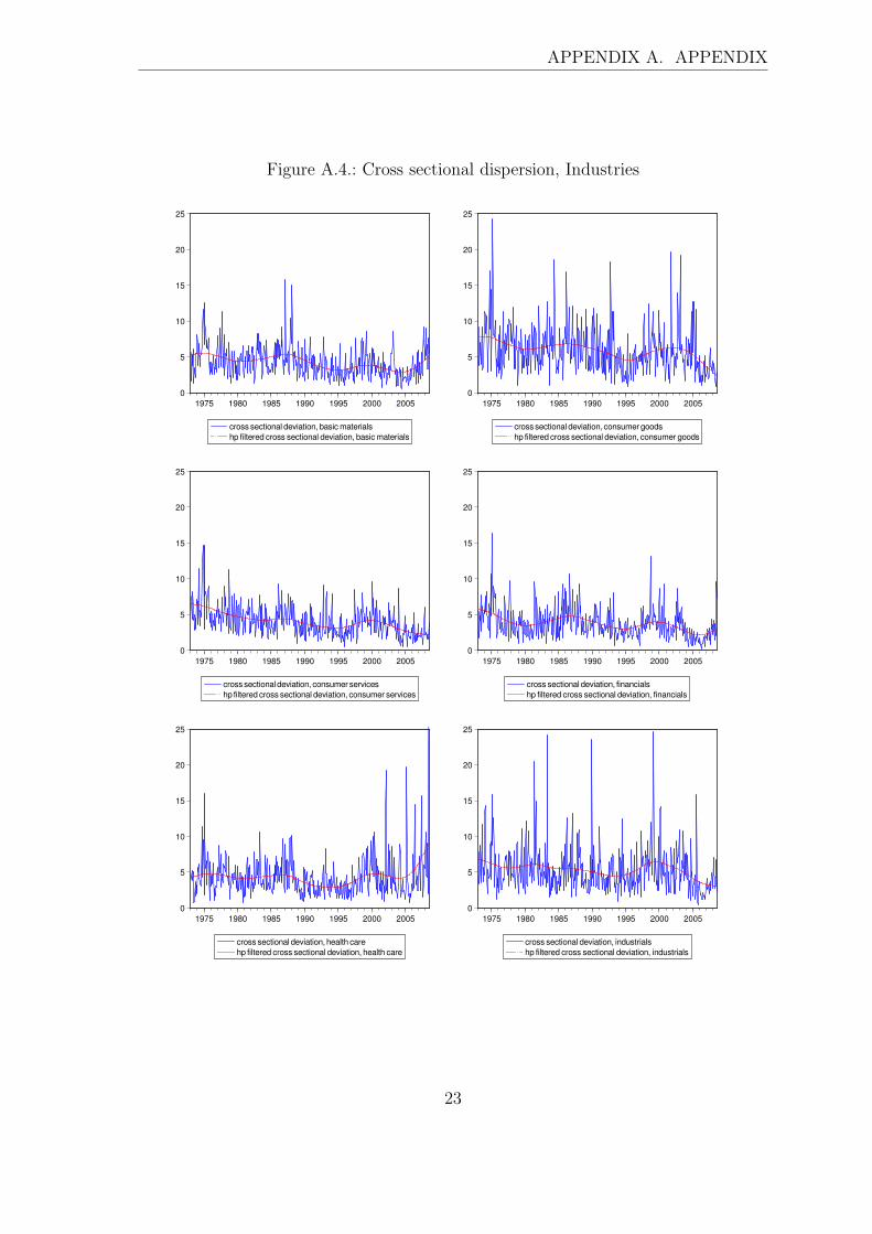
We start our analysis of σ-Convergence by looking at the cross sectional dispersion

across countries at market level. Figure A.3 shows the standard deviation of ag-

gregate market returns across the sample countries and the HP filtered standard

deviation6. The smoothed cross sectional deviation gives us an idea about the long

term trend of convergence. The graph shows that the standard deviation falls evi-

dently but starts to increase in the mid 2000s. When we look at the cross sectional

dispersions for each industry (Figure A.4), we observe that there is a decrease in

volatility in all industries but the trend is not clear for health care industry. An

6λ, the smoothing parameter is taken as 14400 for monthly data.

12


upswing of standard deviations in the mid 2000s is observed for the following indus-

tries: basic materials, financials and health care. We run the equation 2.4 for the

whole sample period to control for the slope coefficient on a linear time trend for

all industries. The results are presented in the last column of Table A.3. The slope

coefficients are all significantly negative at 5 % level accept the slope for health care

industry. The long term trend of cross sectional dispersions has been upward for

health care industry and downward for the other industries.

The evidence of decreasing convergence in the 2000s is just the opposite of what we

expected. There are several arguments, which could have produced this outcome.

First, the origins of the random shocks may be regional. When we consider the

industries, where we observe decrease in convergence in the recent years, we see

that they are generally the ones which may be susceptible to regional shocks; such

as health care and financials. Alternatively, diminishing convergence might be a

result of country-specific economic effect of global shocks. Heterogeneous industrial

structures of countries, differences in the structure of the banking system and in the

credit channel affect the transmission of global shocks to asset values in different ways.

Even if a common monetary policy is fulfilled, the transmission of monetary policy

to economic activity may divert across countries. Finally, if a country becomes more

specialized in an industry, the contents of country indices become different leading

to less synchronized returns. This is in fact consistent with market integration:

different industries may be outstanding in each country. Therefore, economic shocks

may selectively affect specific industries; hence effects on countries may differ. But

a deeper analysis of the reasons behind the presented evidence is beyond the scope

of this paper but leaves room for further research.

We performed a robustness check by analyzing the σ-convergence in two different

episodes of business cycle: recession and expansion. The coefficients are not signif-

icantly different from each other except for health care industry. In this case, the

slope coefficient is positive and significant at 5 % during expansion (0.002) but not

significant during recession. This might suggest that some countries outperform the

others in health care industry during expansionary episodes, which again results from

exposure of health care industry to local shocks.

Finally, Figure A.5 plots the smoothed7 country and industry cross sectional disper-

sions. Country dispersion was higher than that of industry up to the introduction

7HP filtered with a smoothing parameter λ=14400.

13


of euro, hence convergence of returns across industries used to be better than that

of across countries. Together with the introduction of euro, industry dispersion ex-

ceeded country dispersion. Therefore, country convergence of stock market returns

became superior to industry wide convergence in the last stage of EMU.

14

4. Conclusion

This paper’s main objective is to investigate the existence and the degree of con-

vergence among stock markets in Germany, France, Netherlands, Ireland and UK at

the country and industry level considering six different industries: basic materials,

consumer goods, industrials, consumer services, health care and financials. We used

correlation analysis, β-convergence and σ-convergence methods to deal with our ques-

tions. β-convergence serves to measure the speed of convergence and σ-convergence

serves to measure the degree of financial integration.

To summarize our results, stock markets that we studied show an increasing degree of

integration both at the aggregate market level and also at the industry level, although

some differences in the speed and degree of convergence exist among stock markets.

The average half-life of a shock to convergence changes at a range from 5,75 days

for aggregate market to 10,25 days for consumer goods. Convergence has been an

ongoing process since 1973 but the convergence speed has changed from time to time.

There is a decrease in cross sectional dispersions for all industries, however, this is

not the case for health care industry. We do not observe a significant σ-convergence

of health care industry returns, which are more prone to regional shocks.

The finding in this paper should be investigated further. The scope of this paper is

not that extensive to capture the impacts of regional and global shocks on European

stock markets. Future research may explore different sources of shocks on stock

market returns and their affects on convergence.

15

Bibliography

[1] Klaus Adam, Tullio Jappelli, Annamaria Menichini, Mario Padula, and Pagano

Marco.

Analyse, compare, and apply alternative indicators and monitoring methodolo-

gies to measure the evolution of capital market integration in the european

union?

Report to the European Commission, pages 1–95, 2002.

[2] Pierre-Richard Agenor.

Benefits and costs of international financial integration : theory and facts.

Policy Research Working Paper Series 2699, The World Bank, October 2001.

[3] Juan Ayuso and Roberto Blanco.

Has financial integration increased during the nineties?

Banco de Espana, Servicio de Estudios Documento de Trabajo no. 9923, 1999.

[4] Ian Babetskii, Lubos Komarek, and Zlatuse Komarkova.

Financial integration of stock markets among new EU member states and the

euro area.

Czech Journal of Economics and Finance (Finance a uver), 57(7-8):341–362,

2007.

[5] Lieven Baele, Annalisa Ferrando, Peter Hordahl, Elizaveta Krylova, and Cyril

Monnet.

Measuring financial integration in the euro area.

Occasional Papaer Series No. 14, European Central Bank, pages 1–93, 2004.

[6] Markus Baltzer, Lorenzo Cappiello, Roberto A. De Santis, and Simone Man-

ganelli.

Measuring financial integration in new EU member states.

Occasional Paper Series No. 81, European Central Bank, 2008.

16

Bibliography Bibliography

[7] European Central Bank.

Financial Integration in Europe.

April, 2007.

[8] European Central Bank.

Financial Integration in Europe.

April, 2008.

[9] Robert J. Barro and Xavier Sala-i Martin.

Economic Growth.

MIT Press, New York, 1995.

[10] Geert Bekaert and Campbell R. Harvey.

Time-Varying World Market Integration.

Journal of Finance, 50(2), 1995.

[11] Geert Bekaert and Campbell R. Harvey.

Emerging equity market volatility.

Journal of Financial Economics, 2004.

[12] Lorenzo Cappiello, Bruno Gerard, Arjan Kadareja, and Simone Manganelli.

Financial integration of new eu member states.

Working Paper Series, European Central Bank, no. 683, 2006.

[13] Zhiwu Chen and Peter J. Knez.

Measurement of Market Integration and Arbitrage.

Review of Financial Studies, 8(2):287–325, 1995.

[14] Jean-Pierre Danthine and Kpate Adjaoute.

European Financial Integration and Equity Returns: A Theory Based Assess-

ment, pages 185–246.

European Central Bank, Frankfurt, 2003.

[15] Marcel Fratzscher.

Financial market integration in europe: On the effects of emu on stock markets.

International Journal of Finance & Economics, 7(3):165–93, 2002.

[16] Gikas A. Hardouvelis, Richard Priestley, and Dimitrios Malliaropulos.

The Impact of Globalization on the Equity Cost of Capital.

Discussion Paper Series, No. 4346, Centre for Economic Policy Research, 2004.

17

Bibliography Bibliography


EMU and European Stock Market Integration.

Discussion Paper No. 2124, Centre for Economic Policy Research, 79(1), 2006.


EMU and European Stock Market Integration.

Journal of Business, 79(1), 2006.

[19] Kalin Hristov and Rossen Rozenov.

Financial convergence in the new EU member states.

FINESS Working Papers, D.1.2., 2009.

[20] Rene Stulz and G. Andrew M. Karolyi.

Are financial assets priced locally or globally?

Paper No. 2001-11, Dice Center, 2001.

[21] Mark P Taylor and Ian Tonks.

The internationalisation of stock markets and the abolition of U.K. exchange

control.

The Review of Economics and Statistics, 711(2):332–36, 1989.

18

A. Appendix

Table A.1.: Summary Statistics

DE FR NL IE GB DE FR NL IE GBMean Standard Deviation

Market 0,47 0,68 0,55 0,69 0,53 5,12 6,08 4,95 6,53 5,92B. Mater. 0,53 0,94 0,43 0,90 0,67 5,41 6,22 7,50 8,17 6,60Indust. 0,50 0,85 0,39 0,46 0,63 5,65 7,27 8,62 9,94 6,83Cons. Gds 0,38 0,44 0,75 -0,35 0,28 7,03 7,97 7,26 11,85 8,07Hlth Care 0,53 0,71 0,46 1,11 0,76 4,45 6,15 5,64 10,22 5,64Cons. Svs 0,23 0,55 0,57 0,78 0,52 5,80 7,04 5,84 6,91 6,36Finan. 0,49 0,74 0,46 0,74 0,46 6,31 6,09 5,11 7,42 6,40

Figure A.1.: Returns of Aggregate Stock Markets

-5

-4

-3

-2

-1

0

1

2

3

1975 1980 1985 1990 1995 2000 2005

de fr gbnl ie

19

APPENDIX A. APPENDIX

Table A.2.: Correlations of Stock returns with EU benchmark returns

’73m1-’79m2 ’79m3-’90m6 ”90m7-’93m12 ’94m1-’98m12 ’99m1-’08m8Correlation Change in correlation w.r.t. previous period

GERMANYMarket 0,535 0,006 0,278∗ 0,037 0,036B. Mater. 0,460 0,042 0,275∗ -0,012 -0,066Indust. 0,556 -0,131 0,396∗ -0,113∗∗ 0,156∗

Cons. Gds 0,312 0,088 0,334∗ 0,087 -0,020Hlth Care 0,389 0,095 0,184∗ 0,088 -0,141∗∗

Cons. Svs 0,376 0,065 0,210∗ -0,146 0,267∗

Finan. 0,294 0,222∗ 0,240∗ -0,008 0,068FRANCE

Market 0,525 0,049 0,272∗ 0,038 0,046∗

B. Mater. 0,392 0,115 0,326∗ 0,035 -0,150∗∗

Indust. 0,445 -0,025 0,409∗ -0,044 0,063Cons. Gds 0,216 0,264∗ 0,256∗ 0,068 0,020Hlth Care 0,342 0,158∗ 0,127 0,174∗ -0,229∗∗

Cons. Svs 0,418 0,126 0,107 0,107 0,114∗

Finan. 0,362 0,068 0,413∗ -0,025 0,057∗

NETHERLANDSMarket 0,663 0,151∗ -0,058 0,049∗ -0,034B. Mater. 0,632 -0,032 0,122 0,130∗ -0,066Indust. 0,562 -0,016 0,096 0,069 0,146∗

Cons. Gds 0,220 0,204∗ 0,149 0,046 -0,133Hlth Care 0,382 0,268∗ 0,011 0,019 -0,109Cons. Svs 0,374 0,152∗ 0,253∗ -0,027 0,115∗

Finan. 0,688 0,086∗ 0,046 0,009 0,060∗

IRELANDMarket 0,398 0,235∗ 0,084 0,077 -0,163∗∗

B. Mater. 0,355 0,254∗ 0,032 0,094 -0,082Indust. 0,155 0,107 0,316∗ -0,326∗∗ -0,019Cons. Gds 0,197 0,146 0,075 0,165 -0,001Hlth Care NA 0,471 0,032 -0,082 -0,254∗∗

Cons. Svs 0,170 0,407∗ 0,009 -0,003 0,031Finan. 0,594 -0,190∗∗ 0,220∗ 0,124 -0,050

UNITED KINGDOMMarket 0,431 0,160∗ 0,175∗ 0,100∗ -0,048B. Mater. 0,408 0,175∗ 0,168∗ -0,060 0,023Indust. 0,408 -0,017 0,303∗ -0,049 0,147∗

Cons. Gds 0,346 0,065 0,206∗ -0,121 0,118Hlth Care 0,136 0,486∗ 0,027 0,049 -0,099Cons. Svs 0,291 0,216∗ 0,094 0,126 0,070Finan. 0,429 0,137∗ 0,105 0,122∗ 0,073∗

The correlation changes with ” ∗ ” indicate an increase and with ” ∗ ∗” indicate a decrease in correlation coefficients with respect to

the previous period at a significance level of 10%.

20


Table A.3.: β, Half-life and Trend Coefficient Estimates

β-Estimate Half-life (days) Trend Coefficient of σ-ConvergenceMARKET

DE -0,977∗ 5,501FR -1,006∗ 4,039NL -1,047∗ 6,808 -0.007∗

IE -1,021∗ 5,359UK -0,952∗ 6,868

BASIC MATERIALSDE -0,952∗ 6,863FR -1,060∗ 7,384NL -0,975∗ 5,621 -0.005∗

IE -1,077∗ 8,092UK -1,102∗ 9,111

INDUSTRIALSDE -0,943∗ 7,258FR -0,962∗ 6,372NL -0,907∗ 8,771 -0.004∗

IE -1,086∗ 8,460UK -0,974∗ 5,701

CONSUMER GOODSDE -1,169∗ 11,686FR -1,181∗ 12,167NL -0,939∗ 7,438 -0.007∗

IE -1,176∗ 11,970UK -1,075∗ 8,013

HEALTH CAREDE -1,021∗ 5,385FR -0,988∗ 4,670NL -1,058∗ 7,310 0.002∗

IE -1,085∗ 8,444UK -0,946∗ 7,139

CONSUMER SERVICESDE -0,919∗ 8,290FR -0,927∗ 7,957NL -0,965∗ 6,225 -0.008∗

IE -0,865∗ 10,369UK -1,109∗ 9,382

FINANCIALSDE -1,013∗ 4,826FR -1,000∗ 2,500NL -1,061∗ 7,454 -0.005∗

IE -1,048∗ 6,853UK -1,110∗ 9,436

”∗” corresponds 5% significance level.

21


Figure A.2.: Time Varying Estimate of Beta for Germany Market Return

-1.2

-1.0

-0.8

-0.6

-0.4

-0.2

0.0

1975 1980 1985 1990 1995 2000 2005

Market beta for Germany

Figure A.3.: Cross sectional dispersion, Market

0

2

4

6

8

10

12

1975 1980 1985 1990 1995 2000 2005

cross sectional deviation, markethp filtered cross sectional deviation, market

22


Figure A.4.: Cross sectional dispersion, Industries

0

5

10

15

20

25

1975 1980 1985 1990 1995 2000 2005

cross sectional deviation, basic materials

hp filtered cross sectional deviation, basic materials

0

5

10

15

20

25

1975 1980 1985 1990 1995 2000 2005

cross sectional deviation, consumer goods

hp filtered cross sectional deviation, consumer goods

0

5

10

15

20

25

1975 1980 1985 1990 1995 2000 2005

cross sectional deviation, consumer services

hp filtered cross sectional deviation, consumer services

0

5

10

15

20

25

1975 1980 1985 1990 1995 2000 2005

cross sectional deviation, financials

hp filtered cross sectional deviation, financials

0

5

10

15

20

25

1975 1980 1985 1990 1995 2000 2005

cross sectional deviation, health care

hp filtered cross sectional deviation, health care

0

5

10

15

20

25

1975 1980 1985 1990 1995 2000 2005

cross sectional deviation, industrials

hp filtered cross sectional deviation, industrials

23


Figure A.5.: Cross sectional dispersions, Country-Industry Comparison

1.0

1.5

2.0

2.5

3.0

3.5

4.0

4.5

5.0

1975 1980 1985 1990 1995 2000 2005

sector_sd country_sd

24

discussion papers - diw.de

Documents