DISCUSSION PAPER SERIES

ABCD

www.cepr.org

Available online at: www.cepr.org/pubs/dps/DP4324.asp www.ssrn.com/xxx/xxx/xxx

No. 4324

WELFARE REFORM IN EUROPEAN COUNTRIES: A MICRO-

SIMULATION ANALYSIS

Herwig Immervoll, Henrik Kleven, Claus Thustrup Kreiner and Emmanuel Saez

PUBLIC POLICY

ISSN 0265-8003

WELFARE REFORM IN EUROPEAN COUNTRIES: A MICRO-

SIMULATION ANALYSIS

Herwig Immervoll, University of Cambridge and OECD Henrik Kleven, University of Copenhagen and EPRU

Claus Thustrup Kreiner, University of Copenhagen and EPRU Emmanuel Saez, University of California, Berkeley and CEPR

Discussion Paper No. 4324 March 2004

Centre for Economic Policy Research 90–98 Goswell Rd, London EC1V 7RR, UK

Tel: (44 20) 7878 2900, Fax: (44 20) 7878 2999 Email: cepr@cepr.org, Website: www.cepr.org

This Discussion Paper is issued under the auspices of the Centre’s research programme in PUBLIC POLICY. Any opinions expressed here are those of the author(s) and not those of the Centre for Economic Policy Research. Research disseminated by CEPR may include views on policy, but the Centre itself takes no institutional policy positions.

The Centre for Economic Policy Research was established in 1983 as a private educational charity, to promote independent analysis and public discussion of open economies and the relations among them. It is pluralist and non-partisan, bringing economic research to bear on the analysis of medium- and long-run policy questions. Institutional (core) finance for the Centre has been provided through major grants from the Economic and Social Research Council, under which an ESRC Resource Centre operates within CEPR; the Esmée Fairbairn Charitable Trust; and the Bank of England. These organizations do not give prior review to the Centre’s publications, nor do they necessarily endorse the views expressed therein.

These Discussion Papers often represent preliminary or incomplete work, circulated to encourage discussion and comment. Citation and use of such a paper should take account of its provisional character.

Copyright: Herwig Immervoll, Henrik Kleven, Claus Thustrup Kreiner and Emmanuel Saez

CEPR Discussion Paper No. 4324

March 2004

ABSTRACT

Welfare Reform in European Countries: A Micro-Simulation Analysis*

This Paper estimates the welfare and distributional impact of two types of welfare reform in 14 member countries of the European Union. The reforms are revenue neutral and financed by an overall and uniform increase in marginal tax rates on earnings. The first reform distributes the additional tax revenue uniformly to everybody (traditional welfare) while the second reform distributes tax proceeds uniformly to workers only (in-work benefit). We build a simple model of labour supply encompassing responses to taxes and transfers along both the intensive and extensive margin. We then use EUROMOD to describe current welfare and tax systems in all European Union countries (except Sweden) and use calibrated labour supply elasticities along the intensive and extensive margins to analyse the effects of the two welfare reforms. We quantify the equity-efficiency trade-off for a range of elasticity parameters. In most countries, because of the large existing welfare programs with high phase-out rates, the uniform redistribution policy is, in general, undesirable unless the redistributive tastes of the government are extreme. The in-work benefit reform, on the other hand, is desirable in a very wide set of cases. We discuss the practical policy implications for European welfare policy.

JEL Classification: H20 Keywords: labour supply, redistribution and welfare reform

Herwig Immervoll OECD Social Policy Division 2 rue André-Pascal 75775 Paris Cedex 16 FRANCE Tel: (33 1) 45 24 92 14 Fax: (33 1) 44 30 61 78 Email: herwig.immervoll@oecd.org For further Discussion Papers by this author see: www.cepr.org/pubs/new-dps/dplist.asp?authorid=159795

Henrik Kleven Institute of Economics University of Copenhagen Studiestrede 6 DK-1455 Copenhagen DENMARK Tel: (45 35) 32 44 15 Fax: (45 35) 32 30 00 Email: henrik.kleven@econ.ku.dk For further Discussion Papers by this author see: www.cepr.org/pubs/new-dps/dplist.asp?authorid=159550

Claus Thustrup Kreiner Institute of Economics University of Copenhagen Studiestrede 6 DK-1455 Copenhagen DENMARK Tel: (45 35) 32 30 20 Fax: (45 35) 32 30 00 Email: claus.thustrup.hansen@econ.ku.dk For further Discussion Papers by this author see: www.cepr.org/pubs/new-dps/dplist.asp?authorid=154849

Emmanuel Saez University of California, Berkeley 549 Evans Hall, 3880 Berkeley, CA 94720 USA Tel: (1 510) 642 4631 Fax: (1 510) 642 6615 Email: saez@econ.berkeley.edu For further Discussion Papers by this author see: www.cepr.org/pubs/new-dps/dplist.asp?authorid=145017

*We wish to thank Tony Atkinson, Bertil Holmlund, Guy Laroque, David Dreyer Lassen, Thomas Piketty, Steve Pishke, Christian Schultz and numerous seminar participants for helpful comments and discussions, and Nicolaj Verdelin for outstanding computational assistance. The activities of EPRU (Economic Policy Research Unit) are supported by a grant from The Danish National Research Foundation. Any remaining errors and views expressed in this Paper are the authors’ responsibility. In particular, the Paper does not necessarily represent the views of the OECD, OECD member states or the EUROMOD consortium. EUROMOD relies on micro-data from 11 different sources for fifteen countries. These are the European Community Household Panel (ECHP) made available by Eurostat; the Austrian version of the ECHP made available by the Interdisciplinary Centre for Comparative Research in the Social Sciences; the Living in Ireland Survey made available by the Economic and Social Research Institute; the Panel Survey on Belgian Households (PSBH) made available by the University of Liège and the University of Antwerp; the Income Distribution Survey made available by Statistics Finland; the Enquête sur les Budgets Familiaux (EBF) made available by INSEE; the public use version of the German Socio Economic Panel Study (GSOEP) made available by the German Institute for Economic Research (DIW), Berlin; the Survey of Household Income and Wealth (SHIW95) made available by the Bank of Italy; the Socio-Economic Panel for Luxembourg (PSELL-2) made available by CEPS/INSTEAD; the Socio-Economic Panel Survey (SEP) made available by Statistics Netherlands through the mediation of the Netherlands Organisation for Scientific Research – Scientific Statistical Agency; and the Family Expenditure Survey (FES), made available by the UK Office for National Statistics (ONS) through the Data Archive. Material from the FES is Crown Copyright and is used by permission. Neither the ONS nor the Data Archive bear any responsibility for the analysis or interpretation of the data reported here. An equivalent disclaimer applies for all other data sources and their respective providers cited in this acknowledgement. Financial support from the Sloan Foundation and NSF Grant SES-0134946 is gratefully acknowledged.

Submitted 27 February 2004

1 Introduction

Transfers and redistribution towards low income individuals have grown significantly in West-

ern Europe since World War II. Today, as shown in Table 1, most European countries devote

a sizeable amount of public spending to provide low-income support through various programs

such as unemployment insurance for those temporarily out the labor force, disability insurance

for the disabled, housing and families subsidies for those with modest incomes or children, and

various other income maintenance and welfare programs for those with no or very small in-

comes. Table 1 displays the fraction of government transfers in disposable incomes at each

decile for 14 European countries for those aged 18 to 59.1 In all countries, such transfers

represent a very large fraction of disposable income for the bottom deciles.

The proper amount of redistribution and the design of transfer programs is an impor-

tant and controversial issue in the political sphere. As is well known among economists,

redistribution raises the classical equity-efficiency trade-off. Redistribution from middle and

high incomes towards lower incomes is desirable for equity reasons, because society puts a

higher value on the marginal consumption of those with low incomes than on the marginal

consumption of the well-off. However, redistributive programs tend to reduce incentives to

work, thereby creating efficiency costs: to redistribute one additional Euro from high-income

earners to low-income earners, the government needs to impose a welfare cost larger than one

Euro on those with high incomes. Smaller labor supply responses or greater social taste for

redistribution imply that larger transfer programs and higher taxes are desirable.

Following the seminal contribution of Mirrlees (1971) on optimal income taxation, most

studies on labor supply and redistribution issues have focused on the classic two-good static

labor supply model where individuals supply labor so that their indifference curve between

leisure and consumption is tangent to the budget constraint. Most studies on the welfare cost

of taxation have adopted this labor supply model, e.g. Browning and Johnson (1984), Ballard

(1988), and Dahlby (1998). Within this framework, optimal income tax theory shows that

redistribution should take the form of a Negative Income Tax, where a lump-sum transfer

given to everybody is quickly phased out as earnings increase. In this type of welfare program,

1These computations were made using the EUROMOD micro-simulation model described in Section 3 andinclude all types of transfers. The numbers reported are the sum total of per-capita social benefits as apercentage of the sum total of per-capita disposable income. Disposable income is current cash market incomeplus cash social benefits minus taxes and social insurance contributions.

1

transfers to those out of work are financed by positive tax burdens on middle- and high-

income earners. There is a simple trade-off in the design of the program: the size of the

transfer program and the level of taxes on middle and high incomes depends positively on

the strength of redistributive tastes embodied in the social welfare function and negatively on

the size of labor supply responses captured by the elasticity of labor supply with respect to

the net-of-tax wage rate. In this context, the political debate on redistribution is a classical

left-right debate, with the left arguing that redistribution is desirable while the right argues

that labor supply responses are large. We will refer to this debate as the old debate.

However, in this standard model, labor supply depends on the local slope of the budget

constraint and responds only along the intensive margin: hours of work change a little bit

when the marginal tax rate is changed a little bit. This stands in contrast to the political view

blaming welfare programs for keeping individuals or families completely out of the labor force

(see e.g. Murray, 1984). Indeed, a central finding in the empirical labor market literature is

that the extensive margin of labor supply (whether or not to work at all) is more important

than the intensive margin (hours-of-work for those who are working). In particular, extensive

labor supply responses tend to be strong at the bottom of the income distribution (Eissa and

Liebman, 1996; Meyer and Rosenbaum, 2001). Joblessness has long been seen as an important

issue in Europe, where many have blamed high unemployment rates on labor taxes and out-

of-work transfers (see, e.g., Daveri and Tabellini, 2000). The discouraging effects of traditional

welfare programs on participation have lead politicians to advocate programs that preserve

work incentives. Such programs have been developed on a large scale during the 1990s in the

United States through the Earned Income Tax Credit (EITC) and in the United Kingdom

through the Working Families Tax Credit (WFTC). These programs give no support for those

with zero earnings, but provide earnings subsidies for those with low earnings up to a maximum

level above which the program is gradually phased out.

The recent theoretical analysis of Saez (2002) shows that the incorporation of extensive

labor supply responses in the standard Mirrlees model changes the shape of the optimal tax

schedule such that subsidizing the working poor (using negative marginal tax rates at the

bottom) becomes desirable. Therefore, the new debate on welfare reform focuses to a lesser

extent on the size of welfare programs and to a larger extent on the shape of the transfer

programs and the incentives they create in the decision to enter or exit the labor force. The

2

new debate asks whether it is desirable to increase the incentives to work at the bottom by

redistributing from the middle and high income earners to the working poor (instead of to

those with no earnings as in the old debate).

This paper proposes to cast light on the welfare reform debates, both the old debate on

traditional welfare programs and the new debate on redistribution towards the working poor.

We construct a simple and fully explicit model of labor supply encompassing responses along

both the intensive and extensive margins and we then apply the model to the analysis of welfare

reform for 14 European Union countries using the EUROMOD micro simulation model that

has recently become available.

The EUROMOD model is a tax and benefits calculator based on homogeneous micro-data

on income, earnings, labor force participation, as well as many demographic variables, gathered

for 14 of the 15 member countries of the European Union (Sweden is the only EU country

not yet included in the EUROMOD). For any set of household characteristics and country,

EUROMOD is able to calculate the amount of benefits the household is entitled to and the

taxes it should pay. EUROMOD has been constructed to incorporate all the relevant tax and

transfer programs in place in all 14 countries for the year 1998, and is therefore a unique tool

to get a complete picture of the incentives to work generated by those programs as well as the

analysis of welfare reform. An introduction to EUROMOD and a descriptive analysis of taxes

and transfers in the EU countries has been provided by Sutherland (2001), Immerwoll (2002),

and Immervoll and O’Donoghue (2002).

Using the EUROMOD model, we will first provide a brief description of the incentives to

work generated by taxes and transfers along the extensive and intensive margins at each decile

of the earnings distribution for all 14 European countries in the analysis. Second and most

important, we will evaluate the equity-efficiency tradeoff for two simple reforms corresponding

to the old and new debates on welfare reform described above. We calibrate the elasticities

of labor supply along the intensive and extensive margins using estimates from the empirical

literature, and a careful sensitivity analysis will be provided. Like Browning and Johnson

(1984) and others, we measure the equity-efficiency trade-off by the ratio of the dollar value

of the welfare loss for those who lose from the reform to the dollar value of the welfare gain

for those who gain. In other words, we calculate the amount of dollars it would cost the rich

to transfer an additional dollar to the poor (or the working poor).

3

The first reform we analyze corresponds to the old debate. This reform provides a uniform

lump-sum grant to everybody financed by a uniform increase in the marginal tax rate on

earnings for all groups in the population. This reform amounts to the standard NIT-type

program: it provides more support for those with little or no earnings, but at the same time

it weakens the incentives to supply labor along both the intensive and extensive margins.

The second reform corresponds to the new debate. It consists in introducing an EITC-type

program, where the net transfer to those out of work is kept unchanged. A lump-sum grant

provided to all those who are working will be financed by a uniform increase in the marginal

tax rate on earnings. This reform will induce those who are out of work to enter the labor

force (as the rewards for working increase at the bottom of the income distribution), but will

reduce incentives to work along the intensive margin.

For most European countries, expanding the generosity of traditional welfare programs

creates large efficiency costs: redistributing one additional Euro to low incomes by increasing

welfare benefits requires a reduction in the welfare of higher incomes by 2 to 3 Euros on

average (depending on the particular country and the assumed labor supply elasticities). This

is due to the fact that most European countries already impose quite large tax rates on the

participation margin at the bottom of the earnings distribution. By contrast, improving the

incentives to work at the bottom is very cost effective as it will improve incentives to work along

the extensive margin. As a result, the welfare cost of redistributing an additional Euro to the

working poor might be very low (perhaps around 1 Euro, implying no additional deadweight

burden).

Our results stand in significant contrast to previous studies on applied tax/welfare reform in

Europe such as Bourguignon and Spadaro (2002a,b) or in the United States such as Browning

(1995) because we incorporate the extensive margin of labor supply response in the analysis.

The study of Browning (1995), for example, finds that the large EITC program in the United

States is an inefficient way to redistribute income in a classic labor supply model incorporating

only intensive margin responses. Interestingly, the recent study by Liebman (2002) incorpo-

rates fixed costs of work in the Browning model (which amounts to introducing an extensive

margin of labor supply response), and finds that the EITC is a quite efficient redistributive

program in that context. Our results are fully consistent with Liebman’s findings. In contrast

to Liebman, we introduce directly and explicitly extensive elasticities which makes our model

4

more transparent and easier to calibrate using the empirical labor supply elasticity studies.

This paper should perhaps be considered as a first step in the systematic analysis of tax and

benefit reforms in the European Union. We provide a framework which can easily be extended

to consider more complex reform proposals as well as updated to incorporate future findings

from the empirical labor supply research.

The paper is organized as follows. Section 2 lays out the model of labor supply responses

and the theoretical analysis of tax reforms. Section 3 describes the EUROMOD model, the

tax/transfer systems in the 14 European countries we analyze, and applies the theoretical

framework to the practical analysis of welfare reform in each country. Finally, Section 4 offers

some concluding comments, and discusses avenues for future research.

2 Theoretical Analysis

2.1 Labor Supply Responses

In this section, we propose a simple model to capture labor supply responses at both the

intensive and the extensive margins. In order to capture extensive labor supply responses in

a realistic way, it is necessary to introduce non-convexities in either the budget set or the

preferences. In the standard convex model of individual behavior, marginal changes in prices

and endowments give rise to marginal changes in behavior. However, empirical labor market

studies have demonstrated that participation responses are poorly captured within such a

framework (e.g., Blundell and MaCurdy, 1999). Indeed, the empirical evidence indicates that

people choose either to stay out of the labor market or to work at least some minimum number

of hours. Hence, we do not observe infinitesimal working hours for those who enter the labor

market following a marginal increase in the net gain of work, but rather that they enter the

labor force at, say, twenty or forty hours.

In a well-known paper, Cogan (1981) explained these discrete changes in labor supply

behavior by the presence of fixed costs of working and showed empirically that such costs are

important for the labor supply behavior of married women. In Cogan’s analysis, the fixed

costs of working may be monetary costs (say child care expenses), or they may take the form

of a loss of time (e.g., commuting time). Below we adopt a simplified framework where these

two types of fixed costs may be captured in a single parameter q. Within our framework, q

5

may also be interpreted as a distaste for participation/non-participation, or it may reflect the

presence of stigma associated with being out of work. The size of q will be allowed to vary

across individuals.

In addition to heterogeneous fixed costs of working, the model also incorporates heterogene-

ity in abilities and preferences. In particular, we assume that the population may be divided

into J distinct groups with Nj individuals in group j. Across groups, individuals differ with

respect to productivity and preferences. Within each group, individuals are characterized

by identical productivities and preferences, but they differ with respect to their fixed cost of

working. By assuming a continuum of fixed costs, the model will generate a smooth partici-

pation response at the aggregate level of the group, such that we may capture the sensitivity

of entry-exit behavior by setting elasticity parameters for each group.

An individual in group j has an exogenous productivity wj and earns before-tax income

yj = wjl when supplying labor l. The individual faces a non-linear income tax schedule

T (yj , z), where z is an abstract shift parameter which will be used when analyzing tax reforms.

The tax function constitutes a net payment to the public sector, embodying both taxes and

transfers, and therefore −T (0, z) defines the welfare benefit for those not working.The assumption of identical within-group productivities and preferences implies that any

individual who enters the labor market will do so at the same hours of work and earnings

as all the other workers in his own group. While the participation decision is heterogeneous

within the group (from heterogeneous fixed costs), the hours of work and income conditional

on participation are not. Therefore without loss of generality, we may restrict ourselves to

piece-wise linear tax schedules, letting each group face a given marginal tax rate and virtual

income. Thus, we assume that any individual in group j faces the marginal tax rate τ j and has

virtual income Ij . The same type of discrete formulation has been used by Dahlby (1998) to

study the marginal cost of public funds in the standard convex labor supply model. Moreover,

in the context of optimal tax analysis, Saez (2001) has shown that the optimal tax formulas

depend essentially on average labor supply elasticities at each income level, implying that

there is little loss in assuming a discrete set of ability groups, with uniform hours of work and

earnings within each group.

In our static model, income net of taxes and transfers y − T (y, z) is equal to consumption

and is denoted by c. The utility function for an individual in group j with fixed costs of

6

working q, takes the following simple form:

uj(c, l, q) = c− vj (l)− q · 1(l > 0), (1)

where vj(.) is a convex and increasing function normalized so that vj(0) = 0, and 1(.) denotes

the indicator function. In other words, the fixed cost of working q is incurred whenever the

individual decides to start working (l > 0). The above utility specification rules out income

effects on labor supply which is broadly consistent with empirical studies (e.g., Pencavel,

1986) and simplifies considerably the theoretical analysis (Diamond, 1998, and Saez, 2001).

Moreover, even if one was to adopt the view that income effects on labor supply are empirically

large, leaving them out of the analysis is unlikely to be a severe problem in our context because

we will consider only balanced budget reforms. In a balanced budget context, income effects are

quantitatively important for efficiency effects only insofar as they are large and substantially

heterogeneous across different income groups.

The individual chooses l to maximize:

uj(wjl − T (wjl, z), l, q) = wjl − T (wjl, z)− vj (l)− q · 1(l > 0). (2)

In the case of participation, i.e. l > 0, the optimum labor supply choice for an individual in

group j is characterized by

Wj = (1− τ j)wj = v0j (lj) , (3)

where lj denotes hours of work for a participating worker in group j, τ j is the marginal tax

rate for group j, and Wj denotes the net-of-tax wage rate. The optimal hours of work depend

only on the marginal net-of-tax wage rate Wj , not on virtual income. As discussed above, this

implies that the intensive labor supply margin displays no income effects and therefore the

compensated and uncompensated elasticities of labor supply are identical and fully characterize

the intensive labor supply responses. Let us denote by εj the intensive labor supply elasticity

for an individual in group j. By definition, we have

εj =Wj

lj

∂lj∂Wj

. (4)

For the individual to enter the labor market in the first place, the utility from participa-

tion must be greater than or equal to the utility from non-participation. This participation

7

constraint gives rise to an upper-bound on the fixed cost of working, denoted by qj for indi-

viduals in group j. If we denote by cj = wjlj − T (wjlj , z) consumption when working and

by c0 = −T (0, z) consumption when not working, the upper-bound on the fixed cost may bewritten as

qj = cj − c0 − vj (lj) . (5)

Thus, individuals with a fixed cost below the threshold-value qj decide to work lj hours, while

those with a fixed cost above the threshold qj choose to stay outside the labor force (l = 0).

Letting the fixed cost q be distributed according to the distribution function Fj (q) with

density fj(q), the fraction of individuals in group j who choose to participate in the labor

market is given byR qj0 fj (q) dq = Fj (qj). At the aggregate level of group j, participation

depends on qj which reflects the difference in utility between working (supplying lj hours) and

not working (collecting benefits c0) . Like the intensive margin, the extensive labor supply

margin does not display income effects because increasing by the same amount taxes (or

transfers) on those working and on those unemployed does not change the decision to start

working.

Like Saez (2002), we define the extensive elasticity ηj for group j as the percentage change

in the number of workers in group j following a one-percent change in the difference in con-

sumption between working and not working, cj − c0. Formally, we have

ηj =cj − c0Fj

∂Fj∂(cj − c0)

=(cj − c0)fj(qj)

Fj(qj). (6)

We denote by aj = [T (wjlj)− T (0)]/(wjlj) the tax rate on labor force participation. This

tax rate represents the fraction of earnings wjlj that the individual in group j gets to keep

when he decides to enter the labor force and work lj hours. From now on, we call aj the

participation tax rate (as opposed to the marginal tax rate τ j).

The aggregate labor supply of group j is thus equal to

Lj = NjFj(qj)lj . (7)

Hence, the total elasticity of labor supply with changes in the tax schedule can be decom-

posed into the intensive elasticity (affecting the amount of work lj for those working) and the

extensive elasticity (affecting the number of individuals Fj(qj) who decide to work).

8

2.2 The Equity-Efficiency Trade-Off

The goal of this subsection is to study the effects of an arbitrary small tax reform on utili-

ties and tax revenue, and to derive a measure for the marginal trade-off between equity and

efficiency. The effects will be expressed in terms of behavioral elasticities as well as various

parameters of the current tax/transfer system. We then study in more detail two specific types

of tax reform, namely a redistribution through an increase in the demogrant and a redistri-

bution towards the working poor. Finally, we apply this theoretical analysis to 14 European

countries using EUROMOD simulations in Section 3.

Redistributive policies providing income support for the poor or the working poor come at

the cost of reduced incomes and welfare among the high-income earners. In this paper, we will

always consider welfare and tax reforms that are revenue neutral for the government budget.

We will also consider infinitesimal reforms around the current tax and transfer system in order

to keep the analysis as simple as possible. Let us consider a general small and revenue neutral

tax reform dz. This reform creates losers and gainers. Given our utility specification with

no income effects, the marginal utility of money is one for all individuals and welfare gains

and losses can be simply aggregated across individuals. We denote by dG ≥ 0 the aggregatewelfare gains of those who gain from the reform and by dL ≤ 0 the aggregate welfare changeof those who loose from the reform. Note that in the case of a Pareto improving reform there

are no losers and dL = 0.2

Due to behavioral responses to taxes and transfers, the decline in welfare for the rich may

potentially be much higher than the welfare gain for the poor (i.e., dG + dL < 0), reflecting

the distortionary effects of redistributive tax policy. A critical question then becomes how to

evaluate the desirability of reforms involving such interpersonal utility trade-offs. The standard

approach has been to specify a social welfare function involving certain welfare weights across

individuals, say a utilitarian welfare function (with equal weights) or a more egalitarian welfare

function (with decreasing weights across the income distribution). Any given redistributive

policy is then beneficial if it raises the value of the specified social welfare function. However,

the interpersonal comparisons implied by the adopted welfare function are clearly subjective,

and this limits the applicability of such an analysis as an input into the policy making process.

2 In contrast, if the reform is Pareto worsening, there are no gainers and dG = 0.

9

Ideally, we want a measure which does not rely on a priori assumptions about interpersonal

utility trade-offs. In a world of only two types of individuals, such an ideal measure would be

the welfare loss of those who lose relative to the welfare gain of those who gain. This measure

would represent a critical value against which the policy maker may compare his/her subjective

welfare weights to evaluate whether the reform is worthwhile or not. However, the two-type

model does not adequately capture the observed heterogeneity. In our application there will

be many groups of losers and gainers, which complicates matters. Faced with this problem,

we might simply report the welfare effect for each group of individuals, not attempting to

aggregate the group-wise effects into a single aggregate welfare measure. Although it is easy

to consider in our model these disaggregated effects, the paper will focus mostly on a simple

aggregate measure against which to evaluate the reform. It is important to note, however,

that while our reforms are based on individual earnings, welfare is best measured by family

income (for example, a non-working wive with a high income husband is better off than a single

unemployed woman). Therefore, we will examine in some detail the distribution of gainers

and losers when individuals are ranked by family income as opposed to individual income.

Following Browning and Johnson (1984), we divide the population into those who gain from

the reform and those who lose from the reform. This partitioning of people will be endogenous

both to the reform and to the behavioral responses created by the reform. Within each of the

two groups we assume a utilitarian welfare function. We then define the interpersonal utility

trade-off Ψ in the following way

Ψ = − dL

dG. (8)

If the reform in question constitutes an increase in redistribution, Ψ gives the welfare cost to

the rich from the transfer of one additional dollar of welfare to the poor (or the working poor).

Conversely, if we are thinking about rolling back welfare programs, Ψ is the cost to the poor

per dollar transferred to the rich. This interpersonal trade-off may be interpreted as a critical

value for the relative social welfare weight between the two groups, i.e., the relative weight

on those who gain such that the reform breaks even in terms of social welfare. The trade-off

measure used here was originally proposed by Browning and Johnson (1984), and subsequently

used by Ballard (1988) and Triest (1994).

The magnitude of Ψ reflects the degree to which there exists a trade-off between equity

10

and efficiency. In the case with no behavioral responses to taxes and transfers, redistributive

taxation does not imply lower efficiency, and there is no change in aggregate utilitarian welfare

from the reform. Thus, the welfare gain of those who gain (the denominator) exactly equals the

welfare loss of those who lose (the numerator), implying that Ψ is equal to one. Alternatively,

a Ψ-value larger than one implies a trade-off between equity and efficiency (those who lose

from the reform loose more than the gainers gain), whereas if Ψ is less than one there is no

conflict between the two.

To derive Ψ for a general tax reform, we start by examining the impact on individual

utilities from a marginal change in the reform parameter z. From eqs (2) and (3), we obtain

duj (q)

dz=

( −∂Tj/∂z q ≤ qj

−∂T0/∂z q > qj, (9)

where we have introduced Tj ≡ T (wjlj , z) and T0 ≡ T (0, z) to simplify notation. The effect on

individual utility is given simply by the direct change in the tax liability since, by the envelope

theorem, tax-induced changes in hours of work does not affect utility as labor supply is initially

at its optimal level. The marginal utility of income is equal to one for every individual,

due to the quasi-linear specification, and therefore the above utility change is measured in

monetary units.3 While eq. (9) is relevant for all those individuals who are either employed

or unemployed before and after the reform, the welfare effect for those who choose to enter

or exit the labor market following the reform is given by the difference in utilities between

the two states. Since we are considering small reforms, and because the marginal worker is

indifferent between participation and non-participation from equation (5), the welfare effect

for these individuals is not larger than for the rest of the population. Accordingly, as the

group of movers is infinitesimally small for the reforms we consider, we do not have to include

these individuals in our Ψ-measure. This point shows that who decides to enter the labor force

following the small tax reform is actually irrelevant for the welfare analysis. What matters is

who gains and who looses absent any behavioral response. Behavioral responses matter only

for their aggregate effect on tax revenue. We will come back to this important point later on.

Since the reform experiments which we consider do not take money away from those who

are unemployed, i.e. ∂T0/∂z ≤ 0, we may include these individuals among the gainers in the3The result that the welfare effect in monetary units equals the change of tax liability does not hinge on the

quasi-linear specification. This is a general result for marginal reforms following from the envelope theorem.

11

denominator of the Ψ-measure. Moreover, by defining G as the set of ability groups for which

employed people gain from the reform, we may use eq. (9) to write Ψ in the following way

Ψ = −P

j /∈G∂Tj∂z EjP

j∈G∂Tj∂z Ej +

∂T0∂z (N −E)

, (10)

where Ej ≡ Fj (qj)Nj denotes the number of employed people in group j, E =P

j Ej is the

aggregate employment, and N =P

j Nj is the total population.

Since we are considering redistributive policies, the tax reform is revenue neutral. It is

central to note that this does not imply that the partial tax changes in the above expression

sum to zero. Aggregating partial tax changes capture only themechanical effect on government

revenue, i.e., the effect in the absence of behavioral responses. Aggregate government revenue

is given by

R =JX

j=1

[T (wjlj , z)Fj (qj)Nj + T (0, z) (1− Fj (qj))Nj ] , (11)

where the first component reflects tax revenue from employed people, while the second com-

ponent is the (negative) revenue from those who are out of work. A small change in the reform

parameter z affects revenue in the following way

dR

dz=

JXj=1

∙∂Tj∂z

FjNj +∂T0∂z

(1− Fj)Nj + τ jwjdljdz

FjNj + (Tj − T0)dFjdz

Nj

¸. (12)

The revenue effect may be decomposed into mechanical changes (terms one and two) and

behavioral changes along both margins of labor supply (terms three and four). Along the

intensive margin, the reform induces employed people to adjust their hours of work in response

to a changed marginal net-of-tax wageWj . At the same time, some individuals will be induced

to enter or exit the labor market as the reform affects the net-of-tax income gain from entry

cj − c0.

Using eqs (3)-(6), the above expression may be rewritten to

dR

dz=

JXj=1

∙∂Tj∂z

Ej +∂T0∂z

(Nj −Ej)

− τ j1− τ j

∂τ j∂z

εjwjljEj − aj1− aj

∂ (Tj − T0)

∂zηjEj

¸. (13)

For any given reform satisfying dR/dz = 0, we may calculate the equity-efficiency trade-off

Ψ from equation (10). The first two terms in equation (13) are the mechanical effect (which

12

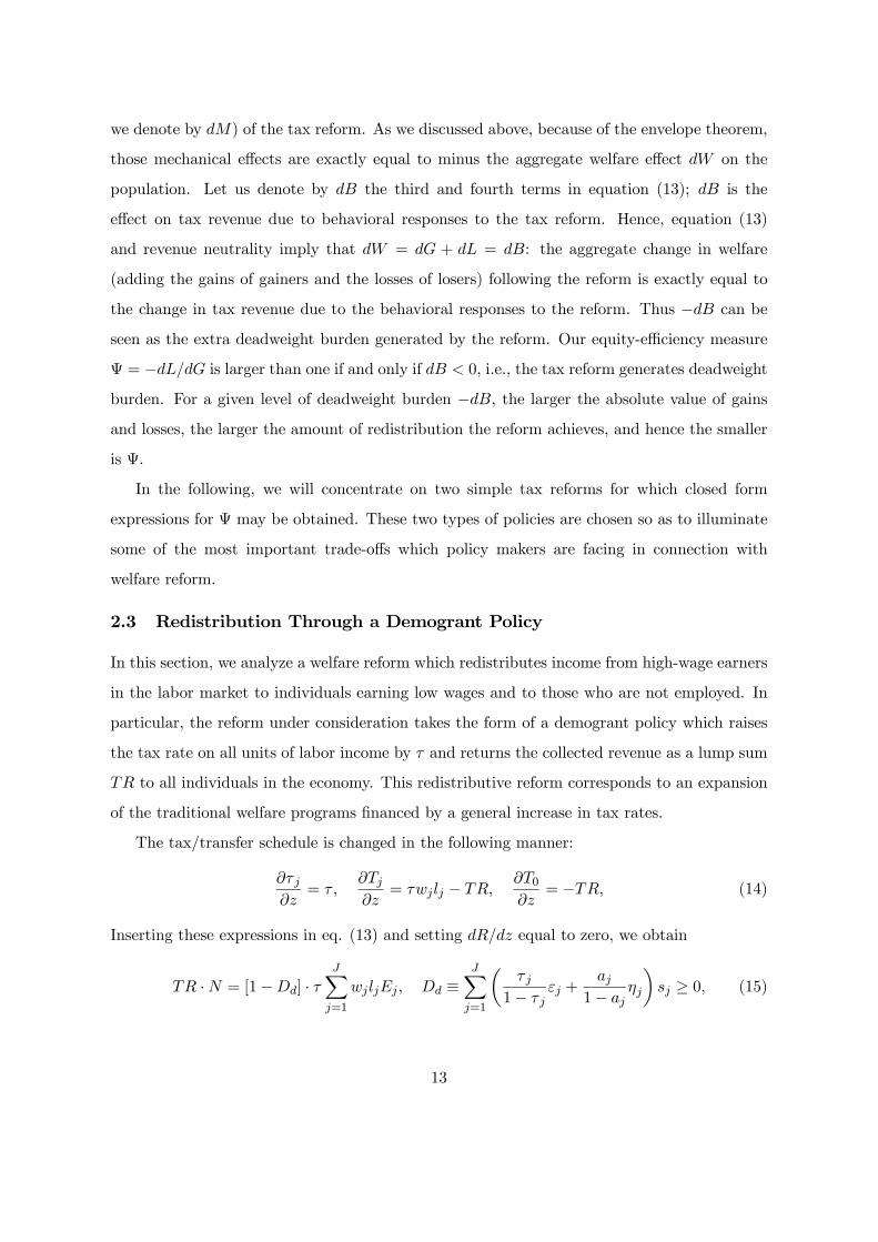
we denote by dM) of the tax reform. As we discussed above, because of the envelope theorem,

those mechanical effects are exactly equal to minus the aggregate welfare effect dW on the

population. Let us denote by dB the third and fourth terms in equation (13); dB is the

effect on tax revenue due to behavioral responses to the tax reform. Hence, equation (13)

and revenue neutrality imply that dW = dG + dL = dB: the aggregate change in welfare

(adding the gains of gainers and the losses of losers) following the reform is exactly equal to

the change in tax revenue due to the behavioral responses to the reform. Thus −dB can be

seen as the extra deadweight burden generated by the reform. Our equity-efficiency measure

Ψ = −dL/dG is larger than one if and only if dB < 0, i.e., the tax reform generates deadweight

burden. For a given level of deadweight burden −dB, the larger the absolute value of gainsand losses, the larger the amount of redistribution the reform achieves, and hence the smaller

is Ψ.

In the following, we will concentrate on two simple tax reforms for which closed form

expressions for Ψ may be obtained. These two types of policies are chosen so as to illuminate

some of the most important trade-offs which policy makers are facing in connection with

welfare reform.

2.3 Redistribution Through a Demogrant Policy

In this section, we analyze a welfare reform which redistributes income from high-wage earners

in the labor market to individuals earning low wages and to those who are not employed. In

particular, the reform under consideration takes the form of a demogrant policy which raises

the tax rate on all units of labor income by τ and returns the collected revenue as a lump sum

TR to all individuals in the economy. This redistributive reform corresponds to an expansion

of the traditional welfare programs financed by a general increase in tax rates.

The tax/transfer schedule is changed in the following manner:

∂τ j∂z

= τ ,∂Tj∂z

= τwjlj − TR,∂T0∂z

= −TR, (14)

Inserting these expressions in eq. (13) and setting dR/dz equal to zero, we obtain

TR ·N = [1−Dd] · τJXj=1

wjljEj , Dd ≡JXj=1

µτ j

1− τ jεj +

aj1− aj

ηj

¶sj ≥ 0, (15)

13

where sj ≡ wjljEj/³PJ

j=1wjljEj

´is group j’s share of aggregate labor income. This ex-

pression shows that the aggregate lump sum transfer TR ·N is equal to the direct increase in

tax revenue from the imposition of τ multiplied by a factor 1 −Dd reflecting the behavioral

responses to the reform. Thus, a fraction Dd of the mechanical tax revenue collections vanishes

due to the behavioral responses to taxation, thereby reducing the amount of money which may

be returned as a lump sum transfer. The fraction Dd is an increasing function of the size of

the labor supply responses measured by the elasticities εj and ηj , and of the size of the tax

rates of the current tax system measured by τ j and aj . Thus, in the special case of no labor

supply responses along either the intensive or the extensive margins (εj = ηj = 0 for all j),

there will be no behavioral revenue loss and therefore Dd equals zero. Likewise, if the initial

tax system is a non-distortionary lump sum tax (τ j = aj = 0 for all j), we get Dd = 0.

Finally, from eq. (15), we note that the revenue (and hence efficiency) effects created

by the two margins of labor supply response are related to different tax wedges. While the

intensive margin is related to the marginal tax rate τ j , the extensive margin is related to the

tax rate on labor market entry aj , which is an average tax rate including any transfers that

are lost or reduced upon labor market entry. This difference between tax/transfer wedges will

be important for the empirical application, a point emphasized by Kleven and Kreiner (2003)

in the context of the marginal cost of public funds.

Now, using eqs (14) and (15), we may rewrite (10) as

Ψd = 1 +Dd

pg(1−Dd)− sg≥ 1, (16)

where pg ≡hP

j∈GEj + (N −E)i/N denotes the population share for those who are gaining

from the reform, while sg ≡P

j∈G sj is the cumulative wage share for those who are gaining.4

If we are considering a tax reform creating no efficiency loss (Dd = 0), the interpersonal trade-

off is exactly one, i.e., an additional dollar transferred to the poor imposes a one-dollar cost

on the rich. However, if the redistributive reform generates an efficiency loss (Dd > 0), and

this is generally the case, it will cost more than one dollar of welfare for the rich to transfer

one dollar to the poor.

4The denominator in eq. (16) captures the welfare gain of those who gain from the reform. Hence, thedenominator is always positive.

14

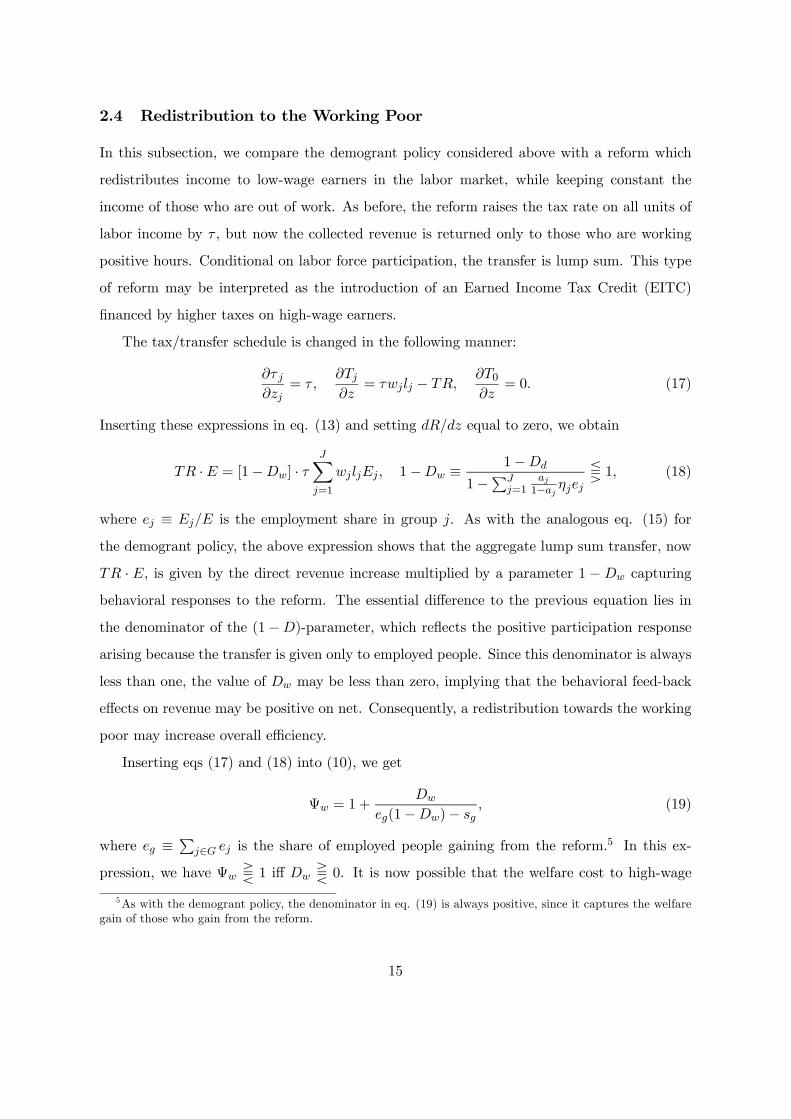
2.4 Redistribution to the Working Poor

In this subsection, we compare the demogrant policy considered above with a reform which

redistributes income to low-wage earners in the labor market, while keeping constant the

income of those who are out of work. As before, the reform raises the tax rate on all units of

labor income by τ , but now the collected revenue is returned only to those who are working

positive hours. Conditional on labor force participation, the transfer is lump sum. This type

of reform may be interpreted as the introduction of an Earned Income Tax Credit (EITC)

financed by higher taxes on high-wage earners.

The tax/transfer schedule is changed in the following manner:

∂τ j∂zj

= τ ,∂Tj∂z

= τwjlj − TR,∂T0∂z

= 0. (17)

Inserting these expressions in eq. (13) and setting dR/dz equal to zero, we obtain

TR ·E = [1−Dw] · τJX

j=1

wjljEj , 1−Dw ≡ 1−Dd

1−PJj=1

aj1−aj ηjej

S 1, (18)

where ej ≡ Ej/E is the employment share in group j. As with the analogous eq. (15) for

the demogrant policy, the above expression shows that the aggregate lump sum transfer, now

TR · E, is given by the direct revenue increase multiplied by a parameter 1 − Dw capturing

behavioral responses to the reform. The essential difference to the previous equation lies in

the denominator of the (1−D)-parameter, which reflects the positive participation response

arising because the transfer is given only to employed people. Since this denominator is always

less than one, the value of Dw may be less than zero, implying that the behavioral feed-back

effects on revenue may be positive on net. Consequently, a redistribution towards the working

poor may increase overall efficiency.

Inserting eqs (17) and (18) into (10), we get

Ψw = 1 +Dw

eg(1−Dw)− sg, (19)

where eg ≡P

j∈G ej is the share of employed people gaining from the reform.5 In this ex-

pression, we have Ψw T 1 iff Dw T 0. It is now possible that the welfare cost to high-wage

5As with the demogrant policy, the denominator in eq. (19) is always positive, since it captures the welfaregain of those who gain from the reform.

15

earners from the transfer of one dollar of welfare to low-wage earners is less than the dollar

transferred. In this case there would be no conflict between equity and efficiency.

In the special case of no labor supply responses along the extensive margin (η = 0), the

two types of tax reform which we have considered create identical behavioral responses (as the

marginal tax rate is increased by τ in each case). It is illuminating to compare our efficiency

and trade-off measures D and Ψ in this special case.

Eqs (15) and (18) show immediately thatDd = Dw, implying that the share of the projected

mechanical increase in tax revenue which is lost through behavioral responses is the same for

the two reforms. In other words, the additional deadweight burden, and hence the difference

between gains dG and losses −dL, is the same for the two reforms. While the differencebetween gains and losses is identical, the absolute magnitudes tend to be higher in the case of

a demogrant policy. In the demogrant policy, the unemployed obtain transfers without paying

any taxes, whereas in the working poor policy everybody getting transfers also pays taxes. For

this reason, the aggregate gain of the gainers dG and the aggregate loss of the losers −dL willbe higher for the demogrant policy. From the definition of the equity-efficiency trade-off in eq.

(8), the larger magnitudes of both numerator and denominator (where the numerator is the

larger number ) implies that Ψd > Ψw, i.e., the demogrant policy involves a more favorable

trade-off than the in-work benefit reform. This result shows that, with no difference in the

behavioral responses created by the reforms, the demogrant policy is “better” than the in-

work benefits policy in the sense that it achieves more redistribution per dollar of deadweight

burden.6

This difference in the trade-off for the two policies is part of a more general point. In

general, the magnitude of Ψ depends on the earnings distribution among the people affected

by the reform. Consider the working poor policy, for example. Since tax payments depend

on earnings, if the distribution of earnings is initially relatively equal (workers are almost

identical), the net mechanical tax change (equal to the welfare effect) will necessarily be almost

the same for each individual (i.e., gains and losses are close to zero). In other words, with

an equal earnings distribution, we get little redistribution, and for a given efficiency loss D,

the trade-off measure Ψ becomes high. As the earnings distribution widens, gains and losses

6This is the main reason why papers analyzing models with only intensive labor supply responses such asBourguignon and Spadaro (2000a,b) or Browning (1995) have found that traditional welfare is preferable toearned income tax credit schemes.

16

become bigger (more money is redistributed), and Ψ becomes lower. This implies that, for

given labor supply elasticities, in-work benefits will be more desirable in countries with large

disparities in earnings.

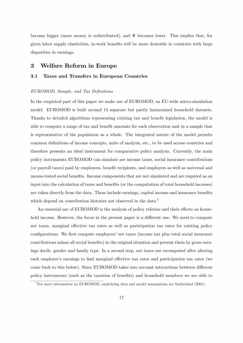
3 Welfare Reform in Europe

3.1 Taxes and Transfers in European Countries

EUROMOD, Sample, and Tax Definitions

In the empirical part of this paper we make use of EUROMOD, an EU-wide micro-simulation

model. EUROMOD is built around 14 separate but partly harmonized household datasets.

Thanks to detailed algorithms representing existing tax and benefit legislation, the model is

able to compute a range of tax and benefit amounts for each observation unit in a sample that

is representative of the population as a whole. The integrated nature of the model permits

common definitions of income concepts, units of analysis, etc., to be used across countries and

therefore presents an ideal instrument for comparative policy analysis. Currently, the main

policy instruments EUROMOD can simulate are income taxes, social insurance contributions

(or payroll taxes) paid by employees, benefit recipients, and employers as well as universal and

means-tested social benefits. Income components that are not simulated and are required as an

input into the calculation of taxes and benefits (or the computation of total household incomes)

are taken directly from the data. These include earnings, capital income and insurance benefits

which depend on contribution histories not observed in the data.7

An essential use of EUROMOD is the analysis of policy reforms and their effects on house-

hold income. However, the focus in the present paper is a different one. We need to compute

net taxes, marginal effective tax rates as well as participation tax rates for existing policy

configurations. We first compute employees’ net taxes (income tax plus total social insurance

contributions minus all social benefits) in the original situation and present them by gross earn-

ings decile, gender and family type. In a second step, net taxes are recomputed after altering

each employee’s earnings to find marginal effective tax rates and participation tax rates (we

come back to this below). Since EUROMOD takes into account interactions between different

policy instruments (such as the taxation of benefits) and household members we are able to

7For more information on EUROMOD, underlying data and model assumptions see Sutherland (2001).

17

capture all relevant effects on total household income of an earnings change for a particular

household member (see Immervoll, 2002 and Immervoll and O’Donoghue, 2002). The tax and

benefit rules we consider are those that were in place in 1998.8

In order to construct ten earnings decile groups, we define our sample as those aged 18

to 59 and who have been working full year and have positive annual earnings. We also ex-

clude those who are currently receiving pension, early retirement, or disability benefits. In all

our tax and benefits simulations, we exclude pension benefits. Deciles are based on pre-tax

earnings (including any social security contributions paid by employers). For our simulations,

we estimate the number of individuals not working using Labour Force Survey employment

participation rates.

The marginal tax rate is computed by increasing actual earnings yj of the individual by

3% and measuring the changes in all taxes and benefits, i.e., τ j = [T (1.03 · yj)− T (yj)] /(0.03 ·yj). In order to compute the participation tax rate, we first compute the difference between

current household taxes and benefits and household taxes and benefits when the earnings of

the individual are set to zero: T (yj)− T (0). We then divide this difference by earnings yj to

obtain the participation tax rate aj = [T (yj)−T (0)]/yj . Marginal tax rates and participation

tax rates by decile for each country are displayed on Figures 1-4.

The theoretical analysis was based on a discrete formulation dividing the population into

J distinct subgroups. In the empirical application, we have to define these subgroups. Here

it is important to choose a level of disaggregation which adequately captures the observed

heterogeneity in the sample. Because tax rates, wage income and (potentially) labor supply

elasticities are strongly heterogeneous and correlated across individuals, one could make sub-

stantial errors by aggregating too much. Our simulations will be based on a disaggregation

into 10 earnings deciles where each decile is divided into 10 subgroups depending on gender

and family type.9 We run simulations where elasticities are allowed to vary across deciles

but are assumed constant across demographic groups within deciles, and we run simulations

where elasticities are heterogeneous across both deciles and demographic groups. In the case of

constant elasticities across demographic groups, we have compared our results from the disag-

8Since 1998, there have been a number of tax and transfer reforms in some of the countries we analyze.9Those ten groups are singles (with no kids), lone parents, married males (no kids and working spouse),

married males (no kids and non-working spouse), married males (kids and working spouse), married males (kidsand non working spouse), married females (no kids and working spouse), married females (no kids and non-working spouse), married females (kids and working spouse), married females (kids and non working spouse).

18

gregated simulation runs (10 deciles × 10 subgroups) to the results from simulation runs wheredemographic subgroups are aggregated. The results turn out to be virtually identical, which

indicates that there is no reason to disaggregate further than we do because of heterogeneity

in tax rates and wage income.10

Typology of Taxes and Benefits

Tables A1 and A2 summarize the main features of taxes and benefits (respectively) affecting

the marginal and participation tax rates of workers in European countries.

All European countries impose three main types of taxes: income taxes, social security

contributions (or payroll taxes), and consumption taxes. Income taxes are levied upon annual

incomes (most of the time both employment and non-employment income with various deduc-

tions), in general with a progressive tax rate structure, and exemption levels. As a result, no

income taxes are paid on very low incomes and marginal income tax rates for high income

households can be substantial.11 Social security contributions (SSC) are levied on employment

and sometimes replacement incomes and in general are designed to finance pensions, health,

and unemployment benefits. They are often shared between employer and the employee and

mostly have a simple flat rate structure with zero payments below a threshold and the con-

tribution base capped above an upper limit. Frequently, thresholds give rise to discontinuities

in the budget set since, once exceeded, the entire income is subject to contributions. Overall

SSC rates can be substantial, especially in countries with large public pension and health in-

surance systems (and often exceed income tax rates).12 Finally, all European countries impose

substantial consumption taxes in the form of Value Added Taxes (VAT) as well as excise taxes

on specific goods (notably cars, gasoline, alcohol, and tobacco). Our tax computations incor-

porate both types of consumption taxes. The consumption tax rate is computed using data

from OECD National Accounts and Revenue Statistics and are reported in Table A3, column

10 It should also be noted that we prefer to carry out simulations disaggregated to the level of decile ×demographic group rather than completely disaggregated to the individual level due to outliers in the sample.Because of discontinuities in the budget sets created by some programs, marginal tax rates may be equal orlarger than one for some individuals, in which case our formulas would be ill defined, and some ad-hoc truncationwould be required.11For example in France in 1998, only half of households are liable to the income tax and the top marginal

income tax rate reaches 54%.12For example, in France for an employee with median earnings, the combined employee-employer SSC mar-

ginal tax rate is over 30%.

19

(3).13 The rates center around 20 percent for most countries, while they are much higher in

Finland and Denmark.

All European governments provide a number of benefits and transfers providing financial

support to individuals and families with certain characteristics such as low income, unem-

ployment, old-age or the presence of children. Benefits depending on income or employment

status can have large effects on budget sets. Low-income groups often face very high marginal

effective tax rates as a result of the tapering of means-tested benefits. We also see frequent

discontinuities caused by work status conditions attached to out-of-work and in-work benefits

or the non-gradual phase-out of benefit payments.14 We describe the main features of the

relevant benefits in Table A2.

We can distinguish five main types of benefits. First, most countries operate social assis-

tance benefits targeted towards those with no or very little income, and tapered away at high

rates. For example, in France, the RMI (Revenu Minimum d’Insertion, or Minimum Income)

provides about 400 Euros per month for a single person with no income and is phased out

at a rate of 100% (above a small earnings disregard). These minimum income benefits may

be almost universal as long as the household meets income conditions (in France the only

requirement is to be above 25), or can be targeted towards specific groups. Minimum income

benefits are often more generous for certain groups such as single parent families, individuals

with disabilities or older individuals (minimum pensions).

Second, a number of benefits are conditional on meeting a number of characteristics and

may not be targeted only to low incomes, although many of them are phased-out with earnings.

For example, many European countries provide housing benefits for families with low incomes.

Family benefits are targeted to households with children or newly born children. In most cases,

family benefits are not means-tested.

Third, a number of European countries provide in-work benefits that are targeted to those

who are currently working or are moving into work. The first European countries to introduce

13The calculation of consumption tax rates is based on the methodology of Mendoza et al. (1994). See thenotes to Table A3 for further details. To account for the effect of consumption taxes on the purchasing powerof labor income, we use the tax rates in Table A3 to adjust the marginal tax rate (τ j) and the participationtax rate (aj). The consumption-adjusted tax rates are given by the formula (TR+CTR)/(1+CTR), where TRis the tax rate exclusive of consumption taxes and CTR is the consumption tax ratio.14For example, in Luxembourg and Belgium (in 1998) housing benefits for single parent families are not

withdrawn smoothly but drop to zero at a specified income threshold.

20

such a program were the United Kingdom and Ireland in the early 1990s. In 1998, the year

on which our study is based, the Family Credit in the U.K. provided a substantial benefit to

all families with children if one parent works at least 16 hours a week and earnings are below

a given modest level.15. Since 1998, a number of other European countries have introduced

in-work benefits. France has introduced such a program as of 2001 (“Prime Pour l’Emploi”

or premium for employment). Belgium is phasing-in an Earned Income Tax Credit program

from 2002 to 2004. The Netherlands have introduced an Employment Tax Credit (since

2001). Germany has introduced in 2002 the “Mainzer Modell” program which is scheduled

to be phased out starting in 2004. Finland is operating an Earned Income Tax Allowance.

In all cases, the new in-work benefits programs in Europe are still small relative to the in-

work benefit programs in the United Kingdom, Ireland, or the United States (see Gradus and

Julsing, 2001). As of 1998, the year on which our simulations are based, only the United

Kingdom and Ireland had introduced significant in-work benefit programs (the Italian family

benefit is dependent on current or previous employment but is not normally considered an

in-work benefit). Therefore and except for those countries, our results can be interpreted as

the welfare analysis of introducing modest in-work benefits programs in a situation where such

programs did not yet exist.

Fourth, all countries operate unemployment insurance benefits which are either temporary

(they expire after some maximum duration) or are conditional on participating in some type

of active labor market program. By definition, unemployment insurance benefits are meant

to replace lost earnings due to job loss until the person finds work again. In our simulations,

computing income measures with and without work requires a special treatment of unemploy-

ment benefits as their duration is limited and not all non-working individuals are currently

receiving them. Therefore, including fully unemployment benefits in the non-working situ-

ation would overstate the value of benefits when out of work. Furthermore, unemployment

benefits, by definition, can only be obtained when one has lost his job. As a result, unemploy-

ment benefits, by narrowing the difference in disposable income when working and when not

working, increase substantially the participation tax rate but have no effect on the marginal

tax rate of those in work. As a result, in the presence of positive labor supply participation

15The United States introduced the Earned Income Tax Credit in the 1970s and this small program wassubstantially expanded in the 1980s and especially the 1990s and has become the largest cash transfer programsfor low income families. The U.S. experience has lead many other countries to adopt similar programs.

21

elasticities, unemployment benefits certainly contribute to making in-work benefits more de-

sirable than the demogrant policy. We adopt the following conservative approach for including

unemployment benefits. For each country as of 1998, we compute the number of unemployed

adults entitled to unemployment benefits using OECD Labour Force Survey statistics on the

unemployed by duration of unemployment and using the duration limits on unemployment

benefits in each country. We then compute the ratio of those unemployment beneficiaries to

the total number of non-working adults aged 18 to 59 in the economy (using again OECD

statistics on the labor force). We then compute marginal and participation tax rates as the

weighted average of the rates estimated including fully unemployment benefits and excluding

fully unemployment benefits. The weight on the scenario with unemployment benefits being

the ratio of unemployment beneficiaries to those non-working, and the weight on the scenario

with no unemployment benefits is one minus this ratio. The resulting ratios are reported for

each of the 14 countries in column (2) of Table A3 in Appendix. In principle, the ideal weight

to use would be the fraction getting unemployment benefits when leaving employment because

of the reform, and the fraction who were getting unemployment benefits among those start-

ing employment because of the reform. Those propensities of getting/loosing unemployment

benefits for the marginal worker/non worker are not observed in the data and we therefore

rely on the propensity of getting benefits for the average person not working. Because those

entitled to unemployment benefits are in principle looking for work, they are perhaps closer

to employment than the average non-working person, suggesting that our measure of unem-

ployment benefits is probably too conservative. In order to assess the sensitivity of our results

to the inclusion of unemployment benefits, we will also provide results in the case where we

exclude completely unemployment benefits (this situation is most favorable to the demogrant

policy relative to the in-work benefits policy and is obviously too conservative).

Finally, all European countries provide public pension benefits. Those benefits are ignored

in the present simulations because we focus on the population aged 18 to 59, and we exclude

from our sample all individuals currently receiving pension benefits.16

Marginal Tax Rates and Participation Tax Rates in Europe

16Gruber and Wise (1999) examine a large number of OECD countries and show that the design of retirementbenefits systems has a strong impact on the retirement decision.

22

Figures 1-4 report the marginal and participation tax rates in the 14 European countries we

study. Countries are divided into two groups of seven countries. The first group is continen-

tal and Northern Europe (Austria, Belgium, Denmark, Finland, France, Germany, and the

Netherlands). As shown on Figures 1 and 3, tax rates for this group are high. The second

group is composed of all the other countries with lower tax rates: Southern Europe (Greece,

Italy, Portugal, and Spain), anglo-saxon European countries (Ireland, the United Kingdom),

and Luxembourg.17

In a number of countries, the structure of tax rates across deciles is strikingly flat. For

example, in the Netherlands the participation tax rate is between 40 and 50% for all deciles.

Belgium, Finland, Germany, Italy, and Portugal have also relatively flat rate structures. This

suggests that, to the extent that decile groups are homogeneous, the tax/transfer system of

those countries is relatively close to a pure Negative Income Tax system combining a demogrant

and a constant marginal tax rate on earnings.

In some countries such as Denmark, participation tax rates are largest at the bottom

because of the existence of relatively generous minimum income benefits which increase the

part of in-work earnings that are effectively "taxed away" upon entering employment. Also,

unemployment benefits are subject to a floor meaning that replacement rates can in some

cases be very high. In contrast, countries such as Greece, Luxembourg, Spain, and the United

Kingdom have relatively lower tax rates at the bottom because minimum income programs

do not exist or are modest relative to in-work earnings, because tax burdens on employment

incomes are small and/or because the operate in-work benefits which counter-balance the loss

of social assistance or unemployment benefits.

Income Distribution

Figures 5-6 displays the P90/P10 and P80/P20 ratios by countries for those with positive

earnings. As is well known, Nordic countries have the lowest level of earnings inequality while

Anglo-saxon countries have the highest. As we discussed above, larger earnings disparities will

make our reforms, and especially the in-work benefit, more desirable as it spreads gains and

losses more widely in the population.

17Luxembourg is of course part of continental Europe. However, as other smaller and very wealthy Europeancountries or principalities such as Lichtenstein or Switzerland, tax rates are significantly lower in Luxembourgthan in other larger continental European countries.

23

3.2 Empirical Literature and Calibration

A central finding in the empirical labor market literature, recently surveyed by Blundell and

MaCurdy (1999), is that labor supply tends to be quite unresponsive along the intensive

margin. While it has long been recognized that the hours-of-work elasticity for prime-age

males is close to zero, more recent research has demonstrated that this is also the case for

females. The old findings of high elasticities for women (especially married women) were

based on censored specifications including non-participating individuals, thereby including the

extensive response in the estimated elasticity. Once labor supply is estimated conditional on

labor force participation, it turns out that the female hours-of-work elasticity is close to that

of males (Mroz, 1987; Triest, 1990).

Hence, a strong degree of labor supply responsiveness would have to come from the margin

of entry and exit in the labor market. Indeed, there is an emerging consensus that exten-

sive labor supply responses may be much stronger than intensive responses (e.g., Heckman,

1993). In particular, participation elasticities seem to be very high for certain subgroups of

the population, typically people in the lower end of the earnings distribution. Let us briefly

review some of the evidence, emphasizing studies based on tax policy experiments which are

our concern here.

One source of evidence comes from a series of Negative Income Tax (NIT) experiments car-

ried out in the United States from the late 1960’s. The empirical results from these experiments

have been surveyed by Robins (1985). The results indicate that participation elasticities are

often above 0.5 and sometimes close to 1 for married women (secondary earners), single moth-

ers, low-educated individuals, and the young. On the other hand, the participation decision

of prime-age males was estimated to be fairly unresponsive to changes in incentives.

More recently, some countries have experimented with various ‘in-work’ benefit reforms for

low income workers. Blundell (2001) describes the reforms and provides a survey of results

from the experiences in the United States, the United Kingdom, and Canada. For the United

States, Eissa and Liebman (1996) and Meyer and Rosenbaum (2001) document that the 1986

expansion of the EITC has had large effects on the labor force participation of single mothers.

This was especially the case for single mothers with low education, where the Eissa-Liebman

study implies an elasticity around 0.6.

24

Like the EITC, the recently implemented Working Families Tax Credit (WFTC) in the

United Kingdom was designed to induce lone mothers from welfare into work. The study by

Blundell et al. (2000) indicate that the reform was quite effective in achieving this goal. They

find that the participation rate of single women with children increased by 2.2 percentage

points (5 per cent). Another interesting source of evidence is provided by the Canadian Self

Sufficiency Programme (SSP), which was structured very much like the EITC and WFTC.

The advantage of the Canadian program lies in the fact that it is a randomized experiment

rather than an actual policy reform, thereby providing an ideal setup to estimate labor supply

behavior. A study by Card and Robins (1998) suggests that this experiment created a very

large increase in labor market attachment. In fact, the treatment group almost doubled their

participation rate over the control group.

The finding that tax incentives may have quite substantial effects on labor force par-

ticipation is consistent with another stream of empirical literature estimating the effect of

out-of-work benefits on unemployment. Krueger and Meyer (2002) survey the evidence from a

number of OECD countries. They conclude that benefits raise the incidence and the duration

of unemployment, and that the elasticity of lost work time with respect to benefits tend to be

around one. Since the risk of unemployment is largest among low-skilled workers, this evidence

also indicates that strong participation responses tend to be concentrated at the bottom of

the wage distribution.

Although the literature on labor supply in anglo-saxon countries is extensive, there are

many fewer studies on labor supply responses for continental European countries. An impor-

tant objection to our method is that elasticities might be substantially smaller in the more

rigid labor markets of continental Europe than in Anglo-saxon countries. Several recent stud-

ies suggest that this is not the case. A number of structural studies of married women labor

supply are surveyed in Blundell and MaCurdy (1999, pp. 1649-1951). Those studies find in

general substantial elasticities (between 0.5 and 1) for most countries (Germany, Netherlands,

France, Italy, and Sweden) although they do not decompose the elasticity into participation

versus hours of work on the job. Blundell (1995) surveys studies of labor market participation

responses in OECD countries and suggests that elasticities for married women are substantial

and similar across countries with values close to 1 (pp. 58-61).

Similarly, Van Soest (1995) and Van Soest et al. (2002) obtain substantial elasticities for

25

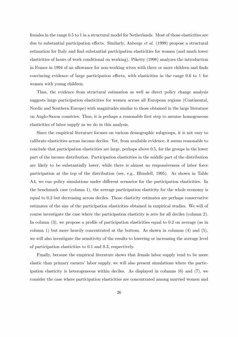
females in the range 0.5 to 1 in a structural model for Netherlands. Most of those elasticities are

due to substantial participation effects. Similarly, Aaberge et al. (1999) propose a structural

estimation for Italy and find substantial participation elasticities for women (and much lower

elasticities of hours of work conditional on working). Piketty (1998) analyzes the introduction

in France in 1994 of an allowance for non-working wives with three or more children and finds

convincing evidence of large participation effects, with elasticities in the range 0.6 to 1 for

women with young children.

Thus, the evidence from structural estimation as well as direct policy change analysis

suggests large participation elasticities for women across all European regions (Continental,

Nordic and Southern Europe) with magnitudes similar to those obtained in the large literature

on Anglo-Saxon countries. Thus, it is perhaps a reasonable first step to assume homogeneous

elasticities of labor supply as we do in this analysis.

Since the empirical literature focuses on various demographic subgroups, it is not easy to

calibrate elasticities across income deciles. Yet, from available evidence, it seems reasonable to

conclude that participation elasticities are large, perhaps above 0.5, for the groups in the lower

part of the income distribution. Participation elasticities in the middle part of the distribution

are likely to be substantially lower, while there is almost no responsiveness of labor force

participation at the top of the distribution (see, e.g., Blundell, 1995). As shown in Table

A4, we run policy simulations under different scenarios for the participation elasticities. In

the benchmark case (column 1), the average participation elasticity for the whole economy is

equal to 0.2 but decreasing across deciles. Those elasticity estimates are perhaps conservative

estimates of the size of the participation elasticities obtained in empirical studies. We will of

course investigate the case where the participation elasticity is zero for all deciles (column 2).

In column (3), we propose a profile of participation elasticities equal to 0.2 on average (as in

column 1) but more heavily concentrated at the bottom. As shown in columns (4) and (5),

we will also investigate the sensitivity of the results to lowering or increasing the average level

of participation elasticities to 0.1 and 0.3, respectively.

Finally, because the empirical literature shows that female labor supply tend to be more

elastic than primary earners’ labor supply, we will also present simulations where the partic-

ipation elasticity is heterogeneous within deciles. As displayed in columns (6) and (7), we

consider the case where participation elasticities are concentrated among married women and

26

lone parents only (with a zero participation elasticity for married men and singles with no

children).

For the hours-of-work elasticity, we will assume that it is constant across income deciles

(like, e.g., Diamond, 1998, and Saez, 2001). We will take an elasticity equal to 0.1 to be our

baseline case, but will also consider values equal to 0 and 0.2.18

3.3 Quantifying the Equity-Efficiency Trade-Off

In this section, we simulate the impact of a demogrant welfare reform and a working poor

welfare reform in EU countries. In order to do so, we combine the theory laid out in Section 2

with the EUROMOD tax and benefit calculations presented in Section 3.1, and setting labor

supply elasticities as described in Section 3.2. Our evaluation of the two types of welfare reform

focuses on economic efficiency and, most importantly, on the trade-off between efficiency and

equality. The pure efficiency effect is measured in proportion of collected revenue and is

found by calculating −D from expressions (15) and (18). The number reflects the fraction of

mechanical tax revenue that is lost due to behavioral responses. A negative value corresponds

to an efficiency loss. The trade-off between efficiency and equality is derived from formulas

(16) and (19). Recall from Section 2 that our measure of the trade-off gives the welfare cost

to the rich from transferring one additional Euro to the poor.

We consider as our baseline case an hours-of-work elasticity equal to 0.1 and a participation

elasticity for the aggregate economy equal to 0.2 in Panel A of Table II (see Table A4 for the

distribution of the participation elasticities across deciles).

Panel A shows that the efficiency implications of welfare reform depend crucially on who

is targeted by the reform, the poor or the working poor. Redistributing income to the poor

by increasing the demogrant leads to efficiency losses in all countries, implying a trade-off

between efficiency and equality above one. Although there is substantial variation across

countries, the equity-efficiency trade-offs tend to be very unfavorable. The smallest trade-offs

are found primarily in Southern Europe and Anglo-Saxon countries where taxes and benefits

are relatively low. In the UK, for example, giving 1 Euro to low-wage earners and those out

18A large literature for the United States has shown that very high income earners might be much moreresponsive to tax rates than middle or middle high income earners (see Saez, 2004 for a recent summary).However, this phenomenon is concentrated at the very top (top 1%) and thus, for our purpose, this high-incomeelasticity should only increase slightly the overall intensive elasticity of the top deciles income earners.

27

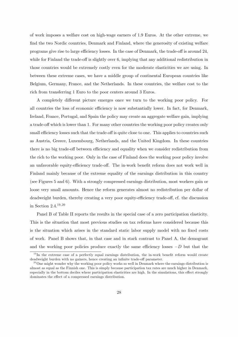
of work imposes a welfare cost on high-wage earners of 1.9 Euros. At the other extreme, we

find the two Nordic countries, Denmark and Finland, where the generosity of existing welfare

programs give rise to large efficiency losses. In the case of Denmark, the trade-off is around 24,

while for Finland the trade-off is slightly over 6, implying that any additional redistribution in

those countries would be extremely costly even for the moderate elasticities we are using. In

between these extreme cases, we have a middle group of continental European countries like

Belgium, Germany, France, and the Netherlands. In these countries, the welfare cost to the

rich from transferring 1 Euro to the poor centers around 3 Euros.

A completely different picture emerges once we turn to the working poor policy. For

all countries the loss of economic efficiency is now substantially lower. In fact, for Denmark,

Ireland, France, Portugal, and Spain the policy may create an aggregate welfare gain, implying

a trade-off which is lower than 1. For many other countries the working poor policy creates only

small efficiency losses such that the trade-off is quite close to one. This applies to countries such

as Austria, Greece, Luxembourg, Netherlands, and the United Kingdom. In these countries

there is no big trade-off between efficiency and equality when we consider redistribution from

the rich to the working poor. Only in the case of Finland does the working poor policy involve

an unfavorable equity-efficiency trade-off. The in-work benefit reform does not work well in

Finland mainly because of the extreme equality of the earnings distribution in this country

(see Figures 5 and 6). With a strongly compressed earnings distribution, most workers gain or

loose very small amounts. Hence the reform generates almost no redistribution per dollar of

deadweight burden, thereby creating a very poor equity-efficiency trade-off, cf. the discussion

in Section 2.4.19 ,20

Panel B of Table II reports the results in the special case of a zero participation elasticity.

This is the situation that most previous studies on tax reforms have considered because this

is the situation which arises in the standard static labor supply model with no fixed costs

of work. Panel B shows that, in that case and in stark contrast to Panel A, the demogrant

and the working poor policies produce exactly the same efficiency losses −D but that the

19 In the extreme case of a perfectly equal earnings distribution, the in-work benefit reform would createdeadweight burden with no gainers, hence creating an infinite trade-off parameter.20One might wonder why the working poor policy works so well in Denmark where the earnings distribution is

almost as equal as the Finnish one. This is simply because participation tax rates are much higher in Denmark,especially in the bottom deciles where participation elasticities are high. In the simulations, this effect stronglydominates the effect of a compressed earnings distribution.

28

demogrant policy produces a more favorable equity-efficiency trade-off as it spreads and gains

and losses more widely among groups, a point we discussed earlier. Those results show that

it can be quite misleading to use the standard labor supply model to study welfare reform for

low income earners if indeed participation elasticities are significant.

To get a better grasp on the difference between the demogrant or working poor policies,

notice from Figures 1-4 that countries with relatively high participation tax rates in the bottom

deciles, such as Denmark, Ireland, or France, tend to gain more by choosing a working poor

policy rather than a demogrant policy. The working poor policy creates, ceteris paribus,

higher incentives for participation in the labor force. Moreover, participation rises mainly

at the bottom deciles where participation elasticities are large. If participation tax rates are

very large at the bottom deciles, the increase in labor participation creates a large increase

in government revenue and hence in economic efficiency. This may be seen more formally by

noting from eq. (18) that

(1−Dd)/(1−Dw) = 1−JX

j=1

aj1− aj

ηjej .

The participation elasticities (ηj) are large at the bottom of the wage distribution while the

employment shares (ej), by definition, are equal to 0.1 for all deciles. Hence, the working poor

policy has a relatively large effect on economic efficiency compared to the demogrant policy if

participation tax rates (aj) are high at the bottom deciles. The same type of mechanism is

at work when we increase the concentration of participation responses in the bottom of the

earnings distribution. As we go from Panel A to Panel C in Table II, the working poor policy

becomes more attractive for all countries, and the effect is largest for those countries imposing

relatively high participation taxes at low wage levels.

In Table III we explore the sensitivity of the results to the average participation elasticity

in the economy. In Panel A the average elasticity equals 0.1, whereas in Panel B the average

elasticity equals 0.3. As one would expect, the overall level of the responsiveness of labor

force participation is very important for the effects of the two policies. A larger elasticity

makes the demogrant policy worse, while it makes the working poor policy better. In the

high-elasticity scenario (Panel B), the working poor policy creates an efficiency gain in most

29

countries, implying a trade-off below 1.21 Although the empirical evidence shows that extensive

responses tend to be larger than intensive responses, we consider the case (in Panel A) of

identical elasticities along the two margins. This scenario constitutes a conservative case for

the working poor policy. It is therefore remarkable that the policy looks more favorable than

the demogrant policy for a fair number of countries.

The sensitivity of the results with respect to the hours-of-work elasticity is analyzed in

Table IV. The analysis indicates that the simulated effects on economic efficiency and equity-

efficiency trade-off seem quite sensitive to the size of the hours-of-work elasticity. However,

unlike the level of the participation elasticity, the hours-of-work elasticity has the same quali-

tative impact on the demogrant policy and the working poor policy. Hence, the relative effects

of the two policies are less influenced by the size of the hours-of-work elasticity.

In Table V, we report results in the same scenarios as in Table II but in the case where we

exclude completely unemployment benefits. We note that the gap between the demogrant and

the working poor policies narrows a little bit but the qualitative implications remain the same.

As long as there are moderate participation elasticities, the current tax and benefits systems,

even ignoring unemployment insurance, imply that the demogrant policy generates more dead-

weight burden and creates a less favorable equity-efficiency trade-off than the working benefits

policy.

Finally, in Table VI, we consider the case where participation elasticities are heterogeneous

within deciles among different demographic groups. We assume that participation elasticities

are concentrated among married women and lone parents and zero otherwise (married men

and singles with no kids). In both Panels A and B of Table VI, the average intensive and

extensive elasticities are 0.1 and 0.2, respectively (as in our benchmark case in Table II). In

Panel B, the participation elasticities are more concentrated in the bottom deciles. Thus, the

results presented in Panels A and B of Table VI ought to be compared with Panels A and C

of Table II. Introducing heterogeneity in the elasticities has only modest consequences on our

efficiency and trade-off measures. The numbers for the working poor policy are very similar

while the demogrant policy looks in general slightly better with heterogeneous elasticities.

However, in all countries, the working poor policy continues to appear more favorable (and

21For Denmark, the demogrant policy generates a Pareto loss (No Gainers) while the working poor policygenerates a Pareto improvement (no Losers). In those cases, the efficiency and efficiency-equity parameters areill defined.

30

often much more favorable) than the demogrant policy suggesting that our results are indeed

very robust to introducing heterogeneity in the elasticities across demographic groups.

3.4 Majority Support and Distributional Effects

Our results strongly suggest that, for most countries and for realistic labor supply elasticity

assumptions, the working poor policy is more desirable than the demogrant policy. This

raises two important questions. First, is the working poor policy more likely to be supported

by a majority of self-interested voters. Second, what are the redistributive consequences of

introducing such a working poor policy?

Columns (1) and (2) of Table VII show the share of gainers for the demogrant and the

working poor policy, respectively, in the case of our benchmark case for elasticities (Table

II, Panel A).22 A majority supports the demogrant policy only in Spain and Italy. In most

countries, especially in the Nordic countries with generous transfer policies, a large majority

would favor rolling back the welfare state (a negative demogrant policy). By contrast, column

(2) shows that, for most countries, the working poor policy would be supported by a majority.23

The reason for those results is again that the in-work benefit creates a low (or no) deadweight

burden and therefore generates more gainers than losers.

The working poor policy hence appears to be economically efficient and also politically

feasible. The last point we examine is the redistributive consequences of such a policy. The

working poor policy benefits workers with low earnings at the expense of higher income earners

(non-workers are left unaffected by the policy). However, the policy has been defined at the

individual level, independent of total family income. Hence, the working poor policy provides

the same benefit to a low income working lone parent and to a low income spouse married to

a high income husband. Therefore, it is conceivable that the redistributive consequences of

the working poor policy are actually much less attractive when total family income is taken

into account. To investigate this point, columns (3) to (7) display the share of individuals

benefitting from the working poor policy in each family disposable income quintile.24 Our

22 In the case of the working poor policy, the non-working population is excluded as it is unaffected by thepolicy.23Only in Belgium, Finland, and Germany would a majority be opposed to the introduction of a working

poor policy.24Hence, in our previous example, the lone parent is likely to be in the first quintile while the spouse of the

high income husband is likely to be in the fifth quintile.

31

results show that, even though some of the gainers are indeed in the top quintile, the fraction

of gainers is always highest in the bottom quintiles. In other words, although some wives

with wealthy husband will gain from the reform, most of the gainers will be individuals with

modest family incomes. Thus, the working poor policy also appears to be redistributing from

high income families toward low income families on average. Finally, it is important to note

that the redistributive properties of the working poor policy (or any other small tax/transfer

change) are independent of the distribution of the behavioral responses. For example, the

policy will have the same redistributive properties even if only wives with wealthy husbands

are induced to work because of the policy and if lone parents are completely inelastic. What

matters in the analysis is the total revenue loss due to all behavioral responses, and the static

redistributive properties of the policy.

4 Discussion

This paper has proposed an analysis of welfare reform in European countries using a simple

static model of labor supply and the EUROMOD micro-simulation model. Following the

findings of the empirical labor supply literature, we have modelled labor supply responses not

only along the intensive margin (as has been done by most previous tax reform studies) but also

along the extensive margin. Our analysis leads to quite definite and robust results. Because

of the presence of significant labor supply responses along the extensive margin, increasing

traditional welfare has very different welfare implications than introducing in-work benefits.

Because of large existing transfer programs which generate significant tax rates for low-wage

earners, increasing redistribution through traditional welfare leads to significant negative labor

supply responses along both the intensive and the extensive margin, thereby creating large

efficiency costs. As we have shown, the welfare cost for high-wage earners from redistributing

one additional Euro to the poor is in the order of magnitude of 2 to 3 Euros. By contrast,

in-work benefits generate positive labor supply responses along the extensive margin (and

the same negative responses along the intensive margin). As a result, the efficiency cost of

redistribution through in-work benefits is much smaller and sometimes very close to zero: in

a number of countries, the welfare cost on higher incomes of redistributing one Euro to the

working poor is actually very close to one Euro.

32

It needs to be emphasized, however, that the groups who benefit from redistribution in

those two reforms are different. In the traditional welfare case, those who benefit the most are

those who have no earnings at all, presumably those who are the most in need of support. In the

in-work benefit case, those with no earnings receive no additional support and redistribution

benefits only the working poor. As a result, if the government had extreme redistributive tastes

and put a much higher welfare weight on those with no incomes than on the working poor

(such as in the case of a Rawlsian welfare criterion), it is possible that increasing traditional

welfare would be more desirable than introducing in-work benefits.25

Our findings are well in line with the recent developments in taxes and benefits in Europe.

As we discussed above, since 1998 (the year upon which our analysis is based), a number of

the European countries have introduced in-work benefits. In year 2003, seven of the fourteen

countries in our sample had implemented in-work benefits programs. Except for Ireland and

the United Kingdom, however, those in-work benefits are still of modest size with maximum

annual benefits between 300 and 1000 Euros (see Gradus and Julsing, 2001, for the most recent

and systematic description of these programs). Therefore, our small reform methodology and

results should in principle provide a good approximation of the effect of introducing such

programs. As illustrated by Blundell (2002) in the case of the extension of in-work benefits

in 1999 in the United Kingdom, such prospective analysis should be supplemented by direct

empirical analysis after the reform. The recent introduction of in-work benefits in several

European countries offers a promising avenue to test our results empirically. Additional and

more precise empirical results would be easy to incorporate into our model to improve the

accuracy of our analysis.

Our simple labor supply model abstracts from a number of issues which we would like to

discuss briefly. First, and perhaps most importantly, we have assumed that the labor market is

perfectly competitive. This might be a poor approximation to European labor markets, where

minimum wages tend to be substantial, and where wage rates are often the result of bargaining

between unions and employers. Minimum wages forbid employers from paying wages which

are below a defined minimum, thereby eliminating jobs with very low productivities and po-

tentially creating involuntary unemployment among the unskilled. Likewise, union bargaining

25By contrast, if the government puts lower welfare weights on those with no earnings than on the workingpoor, the case for in-work benefits would be even stronger. Conservative governments tend to hold the latterview: those not working are seen as lazy, whereas the working poor are seen as deserving.

33

models, efficiency wage models, and search models imply that a fraction of individuals become

involuntary unemployed.

The effects of taxation in imperfect labor markets have been explored in a number of

recent papers (see, e.g., the survey by Sørensen, 1997). The introduction of imperfections

will not change the most important mechanisms at work in our analysis. Firstly, variation

in aggregate employment is still the result of behavioral responses along the intensive and

the extensive margins. For example, Sørensen (1999) considers optimal taxation in three

different models of involuntary employment (unions, efficiency wages, and search) where both

intensive and extensive responses are present. Secondly, in all imperfect labor market models,

a reduction of average tax rates leads to higher employment, where the effect is channelled

through lower equilibrium wages. Accordingly, a working poor policy would lead to increased

job opportunities, while a demogrant policy would reduce the chances of finding a job.26

While the most important employment effects would survive the introduction of labor

market imperfections, the welfare implications of changed labor force participation would be

affected by the presence of involuntary unemployment. Following the introduction of in-work

benefits, those who obtain jobs would experience a discrete (as opposed to an infinitesimal)

increase in utility because some of them were previously involuntarily unemployed. This rein-

forces the positive effect of the working poor policy on welfare. Increasing traditional welfare

programs, on the other hand, creates higher unemployment. To the extent that people lose

their jobs involuntarily, the welfare loss is exacerbated relative to the case of voluntary un-

employment. In conclusion, a model with labor market imperfections generating involuntary

unemployment would most likely increase the attractiveness of redistributing to the working

poor and reduce the attractiveness of increasing traditional welfare programs, thereby rein-

forcing the main conclusion of this paper.

Second, there might be issues related to the presence of segmented labor markets. A well-

known hypothesis is that labor markets tend to have a dual structure, being segmented into

26 In one respect the imperfect labor market models do involve different comparative statics than the com-petitive model. This difference relates to the effect of changes in the marginal tax rate. A higher marginaltax rate (for a given value of the average tax rate) may lead to a lower equilibrium wage rate which, ceterisparibus, imply higher employment. At the same time, higher marginal tax rates give rise to lower workinghours for those who are working as in the standard competitive model. However, the important point to noteis that these effects would apply to both the demogrant and the working poor policies, since both types ofreforms increase the marginal tax rate. The main difference between the reforms lies in their implications forthe average effective tax rates at the bottom of the earnings distribution.

34

a perfectly competitive sector offering low-paying, low-productivity jobs and an imperfectly

competitive sector offering high-paying, high-productivity jobs. Indeed, labor economists have

gathered considerable evidence in favor of the dual labor market hypothesis (see, e.g., the

survey by Saint-Paul, 1996, pp. 62-68). In the dual labor market model, there is a distortion

in the allocation of employment in favor of the perfectly competitive sector offering low-paying

jobs. As pointed out by Bulow and Summers (1986), this implies that the government ought

to use industrial policy to shift resources away from the low-productivity sector. In the con-

text of tax reform, Kleven and Sørensen (2003) show that such sectoral distortions tend to

make policies aimed at the working poor less attractive, because they promote bad jobs at

the expense of good jobs. A policy which succeeds in increasing aggregate employment by

promoting low-paying jobs may, in theory, reduce welfare as it creates a deterioration in the

sectoral mix of employment.

Labor force participation may also generate externalities. Positive externalities of working

would make the introduction of in-work benefits even more attractive relative to traditional

welfare, while negative externalities would make in-work benefits less attractive. Some of

these externalities take the form of fiscal externalities, where higher employment rates affect

the demand for certain commodities that are initially taxed or subsidized by the government.

For example, higher employment may generate more demand for child care, which would then

create positive or negative externalities depending on whether this commodity carries a positive

or negative tax rate (in the Nordic countries, for example, child care is heavily subsidized).

Externalities could also come in the form of social externalities. Positive social externalities

would be reduced crime (as working individuals have less need and time to resort to criminal

activities), newly employed parents being better role models for their children (which could

increase the incentives of children to do well at school, etc.). Negative externalities are also a

possibility if working reduces the time that parents can devote to their children and therefore

worsen the quality of parental education.

Finally, a large body of work in behavioral economics has shown that individuals are not

always able to make the best decisions for themselves, especially when those decisions involve

inter-temporal trade-offs. In the case of labor supply, it is conceivable that some individuals

may not perceive the full future benefits of starting to work, or procrastinate in the decision

to leave welfare and start working. Such models with inconsistent time preferences generate

35

so-called internalities (Herrnstein et al., 1993) that are conceptually close to externalities: an

individual may not internalize fully the utility of future selves and hence decide to work too

little today. As a result, in-work benefits may be desirable to induce people to work more and

help correcting such internalities.

36

References

Aaberge, Rolf, Ugo Colombino and Steinar Strøm (1999). “Labor Supply in Italy:

An Empirical Analysis of Joint Household Decisions, with Taxes and Quantity Constraints.”

Journal of Applied Econometrics, 14, 403-422.

Ballard, Charles L. (1988). “The Marginal Efficiency Cost of Redistribution.” American

Economic Review 78(5), 1019-1033.

Blundell, Richard W. (1995). “The Impact of Taxation on Labor Force Participation and

Labor Supply,” Chapter 3, OECD Job Study: Taxation, Employment, and Unemployment,

OECD: Paris.

Blundell, Richard W. (2001). “Evaluating the Labour Supply Responses to ’In-Work’ Ben-

efit Reforms for Low Income Workers,” in Buti, Marco, Paolo Sestito and Hans Wijkander

(eds.), Taxation, welfare and the crisis of unemployment in Europe. Cheltenham: Edward

Elgar, 157-87

Blundell, Richard W. (2002). “Welfare to Work: Which Policies Work and Why?” Keynes

Lecture in Economics 2001.

Blundell, Richard W. and Thomas MaCurdy (1999). “Labor Supply: A Review of

Alternative Approaches,” in O. Ashenfelter and D. Card (eds.), Handbook of Labor Economics

vol. 3A. Elsevier Science B.V.: Amsterdam.

Blundell, Richard W., Alan Duncan, Julian McCrae and Costas Meghir (2000).

“The Labour Market Impact of the Working Families Tax Credit.” Fiscal Studies 21(1), 75-

104.

Bourguignon, François and Amedeo Spadaro (2002a) “Redistribution and Labour Sup-

ply Incentives: An Application of the Optimal Tax Theory”, mimeo.

Bourguignon, François and Amedeo Spadaro (2002b) “Tax Benefit Revealed Social

Preferences: Are Tax Authorities Non-Paretian?”, mimeo.

Browning, Edgar K. (1995). “Effects of the Earned Income Tax Credit on Income and

Welfare.” National Tax Journal 48(1), 23-43.

Browning, Edgar K. and William R. Johnson (1984). “The Trade-Off between Equality

and Efficiency.” Journal of Political Economy 92(2), 175-203.

Bulow, Jeremy I. and Lawrence H. Summers (1986). “A Theory of Dual Labor Markets

37

with Application to Industrial Policy, Discrimination, and Keynesian Unemployment.” Journal

of Labor Economics 4(3), 376-414.

Card, David and Philip K. Robins (1998). “Do Financial Incentives Encourage Welfare

Recipients to Work?” Research in Labor Economics 17(4), 1-56.

Cogan, John F. (1981). “Fixed Costs and Labor Supply.” Econometrica 49(4), 945-963.

Dahlby, Bev (1998) “Progressive Taxation and the Social Marginal Cost of Public Funds.”

Journal of Public Economics, 67(1), 105-122.

Daveri, Francesco and Guido Tabellini (2000). “Unemployment, Growth and Taxation

in Industrial Countries” Economic Policy 30, 47-88.

Diamond, Peter A. (1998). “Optimal Income Taxation: An Example with a U-Shaped

Pattern of Optimal Marginal Tax Rates.” American Economic Review 88(1), 83-95.

Eissa, Nada and Jeffrey B. Liebman (1996). “Labor Supply Response to the Earned

Income Tax Credit.” Quarterly Journal of Economics 111(2), 605-37.

Gradus, R.H.J.M. and J.M. Julsing (2001). “Comparing Different European Income Tax

Policies Making Work Pay.” Mimeograph OCFEB, Erasmus University Rotterdam.

Gruber, Jonathan, and David Wise (1999). Social Security and Retirement around the

World, University of Chicago Press: Chicago.

Heckman, James (1993). “What Has Been Learned About Labor Supply in the Past Twenty

Years?” American Economic Review Papers and Proceedings 83(2), 116-121.

Herrnstein, Richard J., George E. Loewenstein, Drazen Prelec, and William

Vaughan Jr. (1993). “Utility maximization and melioration: Internalities in individual

choice”, Journal of Behavioral Decision Making, 6, 149-185.

Immervoll, Herwig (2002). “The Distribution of Average and Marginal Effective Tax Rates

in European Union Member States”, EUROMOD Working Paper No. EM2/02.

Immervoll, Herwig, and Cathal O’Donoghue (2002). “Welfare Benefits and Work Incen-

tives: An Analysis of the Distribution of Net Replacement Rates in Europe Using EUROMOD,

a Multi-Country Micro Simulation Model”, EUROMOD Working Paper No. EM4/01.

Kleven, Henrik J. and Claus T. Kreiner (2003). “The Marginal Cost of Public Funds in

OECD Countries: Hours of Work Versus Labor Force Participation.” CESifo Working Paper

no. 935.

Kleven, Henrik J. and Peter B. Sørensen (2003). “Labour Tax Reform, The Good Jobs

38

and The Bad Jobs.” Forthcoming in Scandinavian Journal of Economics.

Krueger, Alan B. and B.D. Meyer (2002). “Labor Supply Effects of Social Insurance,”

in Alan J. Auerbach and Martin Feldstein (eds.), Handbook of Public Economics, vol. 4.

Amsterdam: North-Holland.

Liebman, Jeffrey (2002). “The Optimal Design of the Earned Income Tax Credit”, in Bruce

Meyer and Douglas Hotz-Eakin (eds.), Making Work Pay: The Earned Income Tax Credit and

Its Impact on America’s Families, New-York: Russell Sage Foundation.

Mendoza, E.G., A. Razin, and L.L. Tesar (1994). “Effective Tax Rates in Macroeco-

nomics. Cross-Country Estimates of Tax Rates on Factor Incomes and Consumption.” Journal

of Monetary Economics 34, 297-323.

Meyer, Bruce D. and Dan T. Rosenbaum (2001). “Welfare, the Earned Income Tax

Credit, and the Labor Supply of Single Mothers.” Quarterly Journal of Economics 116(3),

1063-1114.

Mirrlees, James A. (1971) “An Exploration in the Theory of Optimal Income Taxation.”,

Review of Economic studies, 38, 175-208.

Mroz, Thomas A. (1987). “The Sensitivity of an Empirical Model of Married Women’s

Hours of Work to Economic and Statistical Assumptions.” Econometrica 55(4), 765-799.

Murray, Charles (1984). Loosing Ground: American Social Policy 1950-1980. New York:

Basic Books.

OECD (1999) Benefits Systems and Work Incentives, OECD: Paris.

OECD (2002) Revenue Statistics: 1965-2001, OECD: Paris.

OECD (2003) National Accounts, Volume II 1990-2001, OECD: Paris.

OECD (2003) Labor Force Statistics, OECD: Paris.

Pencavel, John H. (1986). “Labor Supply of Men: A Survey,” in O. Ashenfelter and R.

Layard (eds), Handbook of Labor Economics, vol. 1. Amsterdam: North-Holland.

Piketty, Thomas (1998). “L’Impact des Incitations Financières au Travail sur les Comporte-

ments Individuels: Une Estimation pour le cas Français.” Economie et Prevision, 132-133,

1-35.

Robins, Philip K. (1985). “A Comparison of the Labor Supply Findings from the Four

Negative Income Tax Experiments.” Journal of Human Resources 20(4), 567-82.

Saez, Emmanuel (2001). “Using Elasticities to Derive Optimal Income Tax Rates.” Review

39

of Economic Studies 68(1), 205-229.

Saez, Emmanuel (2002). “Optimal Income Transfer Programs: Intensive Versus Extensive

Labor Supply Responses.” Quarterly Journal of Economics 117(3), 1039-1073.

Saez, Emmanuel (2004). “Reported Incomes and Marginal Tax Rates, 1960-2000: Evi-

dence and Policy Implications”, in J. Poterba, ed., Tax Policy and the Economy, Volume 18,

Cambridge: MIT Press.

Saint-Paul, Gilles (1996). Dual Labour Markets: A Macroeconomic Perspective. MIT Press,

Cambridge, Massachusetts.

Sørensen, Peter B. (1997). “Public Finance Solutions to the European Unemployment

Problem?” Economic Policy 25, 223-264.

Sørensen, Peter B. (1999). “Optimal Tax Progressivity in Imperfect Labour Markets.”

Labour Economics 6, 435-452.

Sutherland, Holly (2001). “Final Report EUROMOD: An Integrated European Benefit-Tax

Model”, EUROMOD Working Paper No. EM9/01.

Triest, Robert K. (1990). “The Effect of Income Taxation on Labor Supply in the United

States.” Journal of Human Resources 25(3), 491-516.

Triest, Robert K. (1994). “The Efficiency Cost of Increased Progressivity,” in Joel Slemrod

(ed.), Tax Progressivity and Income Inequality. Cambridge: Cambridge University Press.

Van Soest, A. (1995). “Discrete Choice Models of Family Labor Supply.” Journal of Human

Resources 30, 63-88.

Van Soest, A., M. Das, and X. Gong (2002). “A Structural Labor Supply Model with

Flexible Preferences.” Journal of Econometrics 107, 345-374.

40

Austria Belgium Denmark Finland France Germany Greece Ireland Italy Luxem- Nether- Portugal Spain United Decile Group bourg lands Kingdom

1 42,3% 69,3% 65,4% 74,0% 49,2% 72,6% 29,0% 94,5% 38,0% 41,2% 67,6% 55,0% 48,2% 83,2%2 31,6% 53,3% 62,8% 64,3% 38,7% 45,7% 27,4% 74,2% 37,9% 33,4% 49,2% 28,8% 35,3% 67,9%3 27,5% 31,5% 69,5% 55,7% 29,2% 28,4% 24,2% 63,3% 23,6% 29,5% 33,2% 26,0% 29,1% 52,7%4 27,6% 32,1% 41,1% 43,2% 23,0% 23,8% 15,4% 42,6% 25,6% 25,8% 19,7% 19,2% 28,5% 31,6%5 22,3% 26,2% 27,1% 39,5% 20,2% 17,9% 12,2% 24,3% 20,9% 23,9% 19,4% 15,9% 21,1% 22,6%6 17,0% 23,9% 25,6% 34,7% 18,2% 15,1% 12,4% 16,3% 20,6% 23,4% 12,6% 11,8% 15,6% 12,5%7 19,5% 21,9% 17,1% 29,2% 14,9% 11,0% 18,5% 10,9% 20,6% 16,1% 9,6% 10,8% 15,1% 8,1%8 17,3% 15,0% 13,3% 25,0% 10,8% 9,4% 8,4% 8,5% 20,0% 13,6% 6,1% 14,2% 14,6% 6,4%9 14,9% 12,0% 10,3% 20,5% 10,5% 7,0% 10,2% 5,1% 16,0% 12,1% 7,0% 8,6% 10,1% 3,3%

10 16,7% 10,2% 4,3% 13,1% 8,1% 4,5% 6,5% 1,9% 12,5% 7,0% 4,2% 8,6% 5,8% 1,6%

Total 20,0% 21,2% 20,9% 30,1% 16,4% 15,1% 11,9% 15,7% 19,0% 17,1% 13,9% 13,1% 15,3% 12,9%

Source: EUROMOD tax and benefit calculations.

Table I: Total social benefits over disposable income by deciles in 1998

Note: Decile groups are for per-capita household disposable income. The "modified OECD" equivalence scale is used for computing per-capita figures (with weights 1 for the first adult, 0.5 for further adults and 0.3 for children aged under 14). Working age is 18-59. The table shows, for working age individuals, the sum total of per-capita social benefits as a percentage of the sum total of per-capita disposable income. Disposable income is current cash market income plus cash social benefits minus taxes minus own social insurance contributions.

CountryAustria -0,38 3,04 -0,08 1,50 -0,16 1,57 -0,16 2,16 -0,28 2,29 -0,01 1,04Belgium -0,57 4,83 -0,14 1,93 -0,25 1,87 -0,25 3,45 -0,46 3,41 0,07 0,74Denmark -0,81 23,82 2,87 0,00 -0,23 2,28 -0,23 4,50 -0,82 23,98Finland -0,59 6,33 -0,21 4,82 -0,24 2,11 -0,24 6,32 -0,53 5,24 -0,09 1,83France -0,51 4,32 0,07 0,76 -0,17 1,61 -0,17 2,39 -0,43 3,32 0,26 0,37Germany -0,50 4,38 -0,12 1,89 -0,19 1,72 -0,19 2,67 -0,37 2,91 -0,01 1,08Greece -0,21 1,66 -0,05 1,29 -0,10 1,26 -0,10 1,59 -0,16 1,49 -0,03 1,15Ireland -0,39 2,73 0,26 0,39 -0,14 1,42 -0,14 1,82 -0,34 2,41 0,93 0,07Italy -0,32 2,07 -0,12 1,96 -0,16 1,43 -0,16 2,62 -0,28 1,87 -0,07 1,46Luxembourg -0,26 1,98 -0,06 1,29 -0,12 1,38 -0,12 1,71 -0,20 1,70 -0,03 1,12Netherlands -0,36 2,88 -0,07 1,37 -0,15 1,56 -0,15 2,10 -0,28 2,26 0,03 0,88Portugal -0,29 2,34 0,00 0,99 -0,13 1,44 -0,13 1,68 -0,25 2,05 0,08 0,77Spain -0,19 1,52 0,00 0,99 -0,07 1,16 -0,07 1,34 -0,14 1,38 0,04 0,86United Kingdom -0,22 1,88 -0,01 1,06 -0,09 1,30 -0,09 1,48 -0,17 1,59 0,04 0,86

Source: Authors' own simulations based on EUROMOD tax and benefit calculations.

Notes:η denotes the participation elasticity, and ε denotes the hours-of-work elasticity which is assumed constant across deciles.Efficiency denotes the marginal efficiency cost of the extra-tax used to finance the extra welfare benefits (a negative number is an efficiency loss).Trade-off denotes the ratio of the welfare loss of losers to the welfare gains of gainers from the reform.In Panel A, η =0.4 in deciles 1 and 2, η =0.3 in deciles 3 and 4, η =0.2 in deciles 5 and 6, η =0.1 in deciles 7 and 8, η =0 in deciles 9 and 10.In Panel B, η =0 in all deciles.In Panel C, η =0.8 in decile 1, η =0.6 in decile 2, η =0.4 in decile 3, η =0.2 in decile 4, η =0 in deciles 5 to 10.The tax and benefits computations include a fraction of Unemployment Benefits equal to the ratio of beneficiaries to those non-working.

---- No Losers ----

B. η = 0 and ε = 0.1

Demogrant Policy Working Poor Policy

Efficiency Trade-Off Efficiency Trade-Off Efficiency Efficiency

Working Poor PolicyWorking Poor Policy Demogrant Policy

Trade-Off

η is concentrated more in the bottom deciles

C. η = 0.2 (on average) and ε = 0.1

Table II: Welfare Effects from Tax Reform under Different Profiles for the Participation Elasticity

Efficiency Trade-Off Efficiency Trade-Off Trade-Off

Demogrant Policy

A. η = 0.2 (on average) and ε = 0.1

CountryAustria -0,22 1,90 -0,09 1,57 -0,42 3,47 0,07 0,73Belgium -0,35 2,51 -0,14 2,00 -0,65 6,58 0,42 0,19Denmark -0,52 6,42 0,21 0,35Finland -0,38 3,31 -0,19 3,97 -0,72 10,66 0,02 0,87France -0,30 2,31 -0,04 1,18 -0,62 6,37 1,13 0,04Germany -0,28 2,23 -0,12 1,86 -0,56 5,42 0,11 0,58Greece -0,13 1,37 -0,07 1,37 -0,23 1,75 0,00 1,02Ireland -0,24 1,84 0,13 0,61 -0,47 3,49 2,57 0,00Italy -0,22 1,63 -0,12 2,01 -0,37 2,33 -0,04 1,23Luxembourg -0,16 1,53 -0,08 1,40 -0,28 2,11 0,02 0,93Netherlands -0,22 1,88 -0,08 1,46 -0,41 3,35 0,11 0,61Portugal -0,19 1,72 -0,05 1,18 -0,34 2,69 0,19 0,55Spain -0,11 1,26 -0,02 1,09 -0,21 1,61 0,08 0,71United Kingdom -0,13 1,44 -0,04 1,15 -0,24 2,00 0,09 0,69

Source: Authors' own simulations based on EUROMOD tax and benefit calculations.

Notes:η denotes the participation elasticity, and ε denotes the hours-of-work elasticity which is assumed constant across deciles.Efficiency denotes the marginal efficiency cost of the extra-tax used to finance the extra welfare benefits (a negative number is an efficiency loss).Trade-off denotes the ratio of the welfare loss of losers to the welfare gains of gainers from the reform.In Panel A, η =0.4 in decile 1, η =0.3 in decile 2, η =0.2 in decile 4, η =0.1 in deciles 4, η =0 in deciles 5 to 10.In Panel B, η =0.8 in deciles 1 and 2, η =0.5 in deciles 3 and 4, η =0.2 in deciles 5 and 6, η =0 in deciles 7 to 10.The tax and benefits computations include a fraction of Unemployment Benefits equal to the ratio of beneficiaries to those non-working.

Α. η = 0.1 (on average) and ε = 0.1 Β. η = 0.3 (on average) and ε = 0.1

Efficiency Trade-Off

Demogrant Policy Working Poor Policy

Table III: Welfare Effects from Tax Reform under Different Levels for the Participation Elasticity

---- No Gainers ---- ---- No Losers ----

Demogrant Policy

Efficiency Trade-Off Efficiency Trade-Off

Working Poor Policy

Efficiency Trade-Off

CountryAustria -0,22 1,89 0,15 0,53 -0,53 5,03 -0,31 5,00Belgium -0,32 2,32 0,36 0,23 -0,82 14,78 -0,63 36,55Denmark -0,59 8,21 7,65 0,00Finland -0,35 3,03 0,25 0,27 -0,83 18,52France -0,33 2,54 0,44 0,22 -0,68 8,20 -0,31 5,66Germany -0,31 2,45 0,21 0,38 -0,69 9,17 -0,46 12,20Greece -0,11 1,31 0,06 0,77 -0,30 2,13 -0,17 2,36Ireland -0,25 1,86 0,55 0,16 -0,53 4,18 -0,03 1,12Italy -0,16 1,42 0,10 0,63 -0,49 3,16 -0,33 8,50Luxembourg -0,13 1,41 0,10 0,70 -0,38 2,82 -0,22 2,71Netherlands -0,21 1,82 0,16 0,50 -0,51 4,75 -0,29 4,20Portugal -0,16 1,57 0,19 0,55 -0,42 3,53 -0,18 2,12Spain -0,12 1,30 0,09 0,71 -0,25 1,79 -0,08 1,43United Kingdom -0,13 1,44 0,10 0,66 -0,32 2,49 -0,13 1,76

Source: Authors' own simulations based on EUROMOD tax and benefit calculations.

Notes:η denotes the participation elasticity, and ε denotes the hours-of-work elasticity which is assumed constant across deciles.Efficiency denotes the marginal efficiency cost of the extra-tax used to finance the extra welfare benefits (a negative number is an efficiency loss).Trade-off denotes the ratio of the welfare loss of losers to the welfare gains of gainers from the reform.In both Panels A and B, η =0.4 in deciles 1 and 2, η =0.3 in deciles 3 and 4, η =0.2 in deciles 5 and 6, η =0.1 in deciles 7 and 8, η =0 in deciles 9 and 10.In Panel A, ε =0 in all deciles and in Panel B, ε =0.2 in all deciles.The tax and benefits computations include a fraction of Unemployment Benefits equal to the ratio of beneficiaries to those non-working.

Table IV: Welfare Effects from Tax Reform under Different Levels for the Hours-of-Work Elasticity

Α. η = 0.2 (on average) and ε = 0 Β. η = 0.2 (on average) and ε = 0.2

Demogrant Policy Working Poor Policy Demogrant Policy Working Poor Policy

Efficiency Trade-Off Efficiency Trade-Off

---- No Gainers -------- No Gainers ----

---- No Gainers ----

Efficiency Trade-Off Efficiency Trade-Off

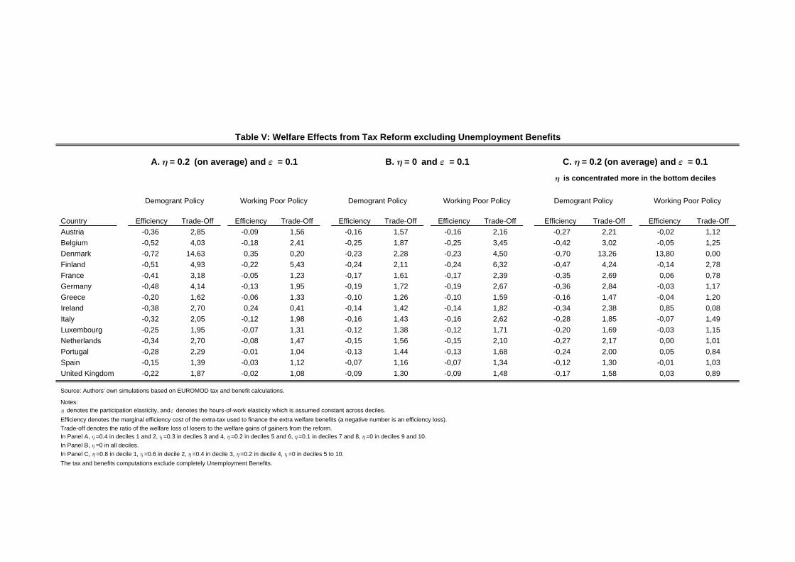
CountryAustria -0,36 2,85 -0,09 1,56 -0,16 1,57 -0,16 2,16 -0,27 2,21 -0,02 1,12Belgium -0,52 4,03 -0,18 2,41 -0,25 1,87 -0,25 3,45 -0,42 3,02 -0,05 1,25Denmark -0,72 14,63 0,35 0,20 -0,23 2,28 -0,23 4,50 -0,70 13,26 13,80 0,00Finland -0,51 4,93 -0,22 5,43 -0,24 2,11 -0,24 6,32 -0,47 4,24 -0,14 2,78France -0,41 3,18 -0,05 1,23 -0,17 1,61 -0,17 2,39 -0,35 2,69 0,06 0,78Germany -0,48 4,14 -0,13 1,95 -0,19 1,72 -0,19 2,67 -0,36 2,84 -0,03 1,17Greece -0,20 1,62 -0,06 1,33 -0,10 1,26 -0,10 1,59 -0,16 1,47 -0,04 1,20Ireland -0,38 2,70 0,24 0,41 -0,14 1,42 -0,14 1,82 -0,34 2,38 0,85 0,08Italy -0,32 2,05 -0,12 1,98 -0,16 1,43 -0,16 2,62 -0,28 1,85 -0,07 1,49Luxembourg -0,25 1,95 -0,07 1,31 -0,12 1,38 -0,12 1,71 -0,20 1,69 -0,03 1,15Netherlands -0,34 2,70 -0,08 1,47 -0,15 1,56 -0,15 2,10 -0,27 2,17 0,00 1,01Portugal -0,28 2,29 -0,01 1,04 -0,13 1,44 -0,13 1,68 -0,24 2,00 0,05 0,84Spain -0,15 1,39 -0,03 1,12 -0,07 1,16 -0,07 1,34 -0,12 1,30 -0,01 1,03United Kingdom -0,22 1,87 -0,02 1,08 -0,09 1,30 -0,09 1,48 -0,17 1,58 0,03 0,89

Source: Authors' own simulations based on EUROMOD tax and benefit calculations.

Notes:η denotes the participation elasticity, and ε denotes the hours-of-work elasticity which is assumed constant across deciles.Efficiency denotes the marginal efficiency cost of the extra-tax used to finance the extra welfare benefits (a negative number is an efficiency loss).Trade-off denotes the ratio of the welfare loss of losers to the welfare gains of gainers from the reform.In Panel A, η =0.4 in deciles 1 and 2, η =0.3 in deciles 3 and 4, η =0.2 in deciles 5 and 6, η =0.1 in deciles 7 and 8, η =0 in deciles 9 and 10.In Panel B, η =0 in all deciles.In Panel C, η =0.8 in decile 1, η =0.6 in decile 2, η =0.4 in decile 3, η =0.2 in decile 4, η =0 in deciles 5 to 10.The tax and benefits computations exclude completely Unemployment Benefits.

Table V: Welfare Effects from Tax Reform excluding Unemployment Benefits

Efficiency Trade-Off Efficiency Trade-Off Trade-Off

Demogrant Policy

A. η = 0.2 (on average) and ε = 0.1

Efficiency Efficiency

Working Poor Policy Demogrant Policy

Trade-OffEfficiency Trade-Off Efficiency Trade-Off

η is concentrated more in the bottom deciles

B. η = 0 and ε = 0.1

Demogrant Policy Working Poor Policy

C. η = 0.2 (on average) and ε = 0.1

Working Poor Policy

CountryAustria -0,29 2,30 -0,05 1,26 -0,25 2,07 -0,01 1,03Belgium -0,51 3,96 -0,03 1,15 -0,43 3,10 0,08 0,69Denmark -0,81 23,75 -0,80 21,13Finland -0,46 4,13 -0,20 4,61 -0,40 3,52 -0,17 3,41France -0,39 2,98 -0,03 1,13 -0,31 2,36 0,03 0,89Germany -0,42 3,38 -0,07 1,40 -0,33 2,59 -0,02 1,10Greece -0,16 1,48 -0,07 1,36 -0,13 1,37 -0,06 1,32Ireland -0,27 1,96 0,02 0,91 -0,23 1,76 0,10 0,69Italy -0,27 1,80 -0,11 1,85 -0,24 1,70 -0,08 1,55Luxembourg -0,20 1,69 -0,06 1,28 -0,18 1,60 -0,04 1,17Netherlands -0,28 2,28 0,02 0,93 -0,26 2,13 0,10 0,62Portugal -0,25 2,08 -0,01 1,04 -0,21 1,85 0,01 0,96Spain -0,14 1,36 -0,01 1,02 -0,12 1,29 0,01 0,95United Kingdom -0,18 1,64 0,00 1,02 -0,14 1,49 0,02 0,92

Source: Authors' own simulations based on EUROMOD tax and benefit calculations.

Notes:η denotes the participation elasticity, and ε denotes the hours-of-work elasticty which is assumed constant across deciles.Efficiency denotes the marginal efficiency cost of the extra-tax used to finance the extra welfare benefits (a negative number is an efficiency loss).Trade-off denotes the ratio of the welfare loss of losers to the welfare gains of gainers from the reform.For lone parents and married women, the participation elasticities are as follows:In Panel A, η =0.9 in deciles 1 and 2, η =0.6 in deciles 3 and 4, η =0.4 in deciles 5 and 6, η =0.2 in deciles 7 and 8, η =0 in deciles 9 and 10.In Panel B, η =1.5 in decile 1, η =1.0 in decile 2, η =0.5 in decile 3, η =0.3 in decile 4, η =0 in deciles 5 to 10.For all other groups (singles and married men), the participation elasticities are zero.In both Panels A and B ε =0.1 in all deciles.The tax and benefits computations include a fraction of Unemployment Benefits equal to the ratio of beneficiaries to those non-working.

Married Women and Lone Parents Table VI: Welfare Effects from Tax Reform where the Participation Elasticities are Concentrated on

---- No Losers ---- ---- No Losers ----

η is concentrated more in the bottom deciles

Α. η = 0.2 (on average) and ε = 0.1 Β. η = 0.2 (on average) and ε = 0.1

Demogrant Policy Working Poor Policy Demogrant Policy Working Poor Policy

Efficiency Trade-Off Efficiency Trade-Off Efficiency Trade-Off Efficiency Trade-Off

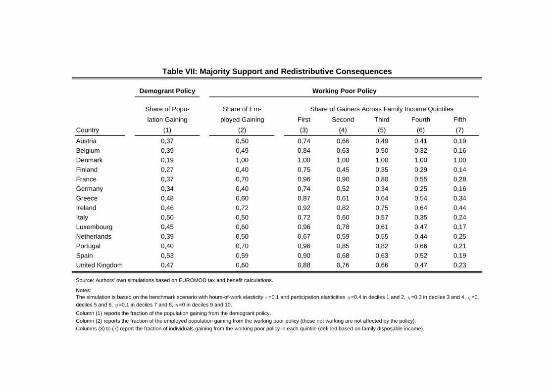
First Second Third Fourth FifthCountry (3) (4) (5) (6) (7)

Austria 0,74 0,66 0,49 0,41 0,19Belgium 0,84 0,63 0,50 0,32 0,16Denmark 1,00 1,00 1,00 1,00 1,00Finland 0,75 0,45 0,35 0,29 0,14France 0,96 0,90 0,80 0,55 0,28Germany 0,74 0,52 0,34 0,25 0,16Greece 0,87 0,61 0,64 0,54 0,34Ireland 0,92 0,82 0,75 0,64 0,44Italy 0,72 0,60 0,57 0,35 0,24Luxembourg 0,96 0,78 0,61 0,47 0,17Netherlands 0,67 0,59 0,55 0,44 0,25Portugal 0,96 0,85 0,82 0,66 0,21Spain 0,90 0,68 0,63 0,52 0,19United Kingdom 0,88 0,76 0,66 0,47 0,23

Source: Authors' own simulations based on EUROMOD tax and benefit calculations.

Notes:

Column (1) reports the fraction of the population gaining from the demogrant policy.Column (2) reports the fraction of the employed population gaining from the working poor policy (those not working are not affected by the policy).Columns (3) to (7) report the fraction of individuals gaining from the working poor policy in each quintile (defined based on family disposable income).

The simulation is based on the benchmark scenario with hours-of-work elasticity ε =0.1 and participation elasticities η =0.4 in deciles 1 and 2, η =0.3 in deciles 3 and 4, η =0.deciles 5 and 6, η =0.1 in deciles 7 and 8, η =0 in deciles 9 and 10.

lation Gaining ployed Gaining(1)

1,000,270,370,34

0,370,39

0,500,49

0,500,460,48

0,47

0,500,450,390,400,53

0,70

Demogrant Policy

Share of Popu- Share of Em-

Working Poor Policy

Share of Gainers Across Family Income Quintiles

0,19

(2)

0,59

Table VII: Majority Support and Redistributive Consequences

0,40

0,60

0,700,400,600,72

0,600,50

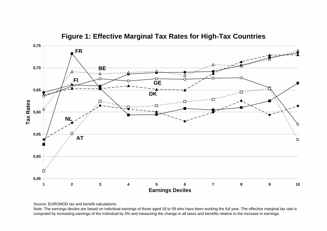
Figure 1: Effective Marginal Tax Rates for High-Tax Countries

0,45

0,50

0,55

0,60

0,65

0,70

0,75

1 2 3 4 5 6 7 8 9 10Earnings Deciles

Tax

Rat

es

FI

BE

GE

FR

AT

DK

NL

Source: EUROMOD tax and benefit calculations.Note: The earnings deciles are based on individual earnings of those aged 18 to 59 who have been working the full year. The effective marginal tax rate iscomputed by increasing earnings of the individual by 3% and measuring the change in all taxes and benefits relative to the increase in earnings.

Figure 2: Effective Marginal Tax Rates for Low-Tax Countries

0,15

0,20

0,25

0,30

0,35

0,40

0,45

0,50

0,55

0,60

0,65

1 2 3 4 5 6 7 8 9 10Earnings Deciles

Tax

Rat

es

SP

UK

GR

LU

PT

ITIR

Source: EUROMOD tax and benefit calculations.Note: The earnings deciles are based on individual earnings of those aged 18 to 59 who have been working the full year. The effective marginal tax rate is computed by increasing earnings of the individual by 3% and measuring the change in all taxes and benefits relative to the increase in earnings.

Figure 3: Participation Tax Rates for High-Tax Countries

0,45

0,50

0,55

0,60

0,65

0,70

0,75

0,80

0,85

1 2 3 4 5 6 7 8 9 10Earnings Deciles

Tax

Rat

es

FI

BE

AT

FR

DK

GE

NL

Source: EUROMOD tax and benefit calculations.Note: The earnings deciles are based on individual earnings of those aged 18 to 59 who have been working the full year. The participation tax rate is computed by setting earnings equal to zero and measuring the change in all taxes and benefits as a share of the actual earnings of the individual.

Figure 4: Participation Tax Rates for Low-Tax Countries

0,30

0,35

0,40

0,45

0,50

0,55

0,60

0,65

0,70

1 2 3 4 5 6 7 8 9 10Earnings Deciles

Tax

Rat

es

SP

UK

PT

PT

IT

LU

GR

IR

Source: EUROMOD tax and benefit calculations.Note: The earnings deciles are based on individual earnings of those aged 18 to 59 who have been working the full year. The participation tax rate is computed by setting earnings equal to zero and measuring the change in all taxes and benefits as a share of the actual earnings of the individual.

Figure 5: Earnings Inequality

1

2

3

4

5

6

7

FI DK IT FR GR GE LU SP AT BE PT NL IR UK

Countries

90th

Per

cent

ile R

elat

ive

to 1

0th

Perc

entil

e

Source: EUROMOD calculations.Note: The earnings deciles are based on individual earnings of those aged 18 to 59 who have been working the full year.

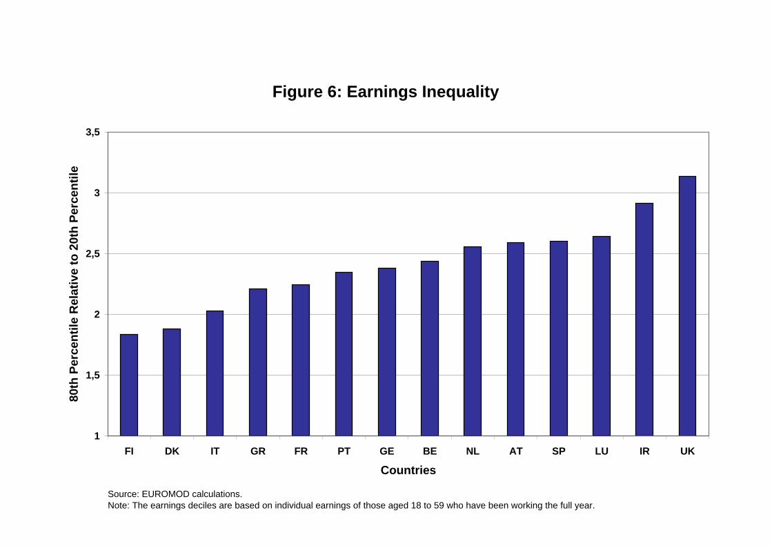
Figure 6: Earnings Inequality

1

1,5

2

2,5

3

3,5

FI DK IT GR FR PT GE BE NL AT SP LU IR UK

Countries

80th

Per

cent

ile R

elat

ive

to 2

0th

Perc

entil

e

Source: EUROMOD calculations.Note: The earnings deciles are based on individual earnings of those aged 18 to 59 who have been working the full year.

Table A1: Taxes on workers, 1998 (rates shown for a single full-time blue-collar private sector employee with no other income and no non-standard expenses)

VAT Income Tax7 employee SSC employer SSC

standard rate [%]

lowest/highest tax band limit1,2

lowest/highest rate [%] main tax credit1 tax unit family-related tax provisions

thres-hold1 rate [%] ceiling1 tax

deductiblethres-hold1 rate [%] ceiling1 taxable features reducing METR features increasing METR

Austria 20 17/231 21/504 rates 5 individual deduction for single earners;

tax credits for lone parents 15 18.8 193 yes 15-

21.34.5

49000- no for a 2nd earner: phase-out of single-earner

credit

Belgium 21 24/318 25/557 rates - individual

parts of taxable income transferrable to spouse;

additional tfa for children and lone parents

- 11.9 - yes - 45.4 - no for a 2nd earner: phase-out of amount transferrable from higher-earning spouse

Denmark 25 12/100 40/594

3 rates- individual unused deductions

transferrable to spouse - 9+ flat amnt - yes - 2.0

+ flat amnt - no

Finland 22 35/223 24/564

6 rates- individual -

587.60.5 - yes - 24.5 - no earned income tax allowance of 20% of

taxable earnings above 11

phase out of earned income tax allowance for earnings > 31; and basic allowance for

taxable earnings > 76

France 20.6 30/336 11/546 rates - family

---

136-

0.99.62.84

3.67.6

-136409545

-

yesyesyesyes

partly

---

136

19.813.44.15.3

-136409545

noreductions of marginal employer

contributions rates of up to about 60% for wages < 130% min. wage.

Germany 1630

133252

27.337.255.75

- family choice of tfa or child benefit 15 7.713.4

156208 yes 15 7.7

13.4156208 no

Greece 18 56/478 5/455 rates

max. 15% of accepted hshld.

expendit.individual 0.9-1.8 non-refundable tax

credit per child - 15.9200;

none for new jobs

yes - 28.2200;

none for new jobs

no

Ireland 21 25/80 24/462 rates -

family (individual optional)

- 4186

4.52.3

193- no

-112

-

8.512.04.0

12231231

no tax reduced to zero for income below 33 (higher limit if children) tax reduction phased out above the 33 limit.

Italy 20 0/118 19/465 rates up to 6 individual up to 2 tax credit per

dependent family members-

569.04

1- yes - 33.04 - no

for 2nd earner: tax credit for dependent spouse phased out; main tax credit slowly

phased out for incomes > 30

Luxembourg 15 25/250 6/4717 rates - family

deductions for lone parents and care expenditure; 3 tax

credit per child- 13.1 259 yes - 14.64 259 no for 2nd earner: 17 additional (joint)

deduction if both spouses work

Netherlands 17.5 20/212 368/603 rates

- individual additional 1240 tfa for lone parents

54-

5.31.7

156105

yesno

54--

6.45.67.94

156105156

noyesno

Portugal 17 0/490 59/405 rates

3 family additional 1.5 tax credit per child - 11 - no - 23.8 - no

Spain 16 22/492 20/568 rates 3

family (individual optional)

up to 2 tax credit per child (plus additional amounts in

some regions)46 30.8 177 yes 46 6.4 177 no earners if income below 55 are exempt

from tax

"spike" in METR once above exemption limit; phase out of main tax credit adds 5 pct.

points to METR

United Kindgom

17.5 29/220 20/403 rates - individual

2 tax credit for married couples; 13 tax deduction for

lone parents23 8.4 to 10 177 no

2310

405676

357

10

- no

6 West Germany

5 Including "Solidarity Surplus Tax" for German unification. MTR increases linearly inbetween lower and middle; and middle and top tax band limits.

4 averages: rates differ between municipalities and/or employers

Notes: tfa = tax free allowance1 in % of median gross employment income (not including employer social security contributions)2 after adding any standard tax free allowances, deductions or exemptions available to single employees3 insurance is voluntary

7 including regional income taxes where applicable8 including pension contributions (same tax base as income tax)9 effective rate taking into account the allowance of 70% of the tax base for low incomes10 all earnings are subject to the applicable rate once they exceed these threshold levels

Table A2: Social Benefits available to persons of working-age, 1998 (rates shown for single benefit recipients)Social Assistance Housing Benefit Family Benefits In-work Benefits Unemployment Benefits2

max. amount1 disregard1 withdrawal rate taxable max. amount1 withdrawal rate amount1 withdrawal rate amount1 work/income conditions withdrawal rate floor rate; amount ceiling taxable

Austria 32 - 100% IT: noSSC: no - - 5-7 per child - - - - 7 55% of net min(56, 80%

of net)IT: no

SSC: no

Belgium 39 9 100% IT: noSSC: no - - 4-13 per child; additional

supplements if not working - - - -31 (if

previous job full-time)

60% of gross48 (if

previous job full-time)

IT: reducedSSC: no

Denmark 34 (+ housing allowance) up to 9 100% IT: yes

SSC: no3 (no children); 14

(>3 children) 75%3-4 per child; higher for one

parents; plus day-care subsidy

- - - -56 (if

previous job full-time)

90% of (gross minus SSC) 68 IT: yes

SSC: partly

Finland 18 (+reasonable housing cost) - 100% IT: no

SSC: no 17 80%5-9 per child; plus 2 per

child for lone parents; plus day-care subsidy

- - - - 22 up to 42% of net exceeding 22 - IT: no

SSC: no

France24; (plus lone

parent benefit of 31+10 per child)

- 100% IT: noSSC: no ca. 15 ca. 34%

main benefit: 7 to 12 for second & further children; special benefits for young

children

main benefit: 100% once income > 174-

261- - - 30 57-75% of gross 313 IT: yes

SSC: yes

Germany 133 4 75-100% IT: noSSC: no ca. 25 ca. 40%

5-9 per child; plus 5-7 child raising benefits for very

young children

young child raising benefit: 20-40%

once income > 62- - - - 60% of net 125 IT: no

SSC: no

Greece - - - - - - 0.5-1 per child plus additions for large families

reduced in steps for incomes > 65 - - - 28 40-70% of gross min(126, 70%

of gross)IT: reduced

SSC: no

Ireland 29 (+housing supplements)

19 for partner's income

100% IT: noSSC: no 3-4 per child -

60% of difference between family gross earnings and ca.

88 (higher limit for larger families)

couple jointly working at least 20 hours per week

60% (of gross earnings) -

138 to 305 depending on previous gross

earnings- IT: reduced

SSC: no

Italyca. 3-17 per family member (also spouses) depending on

family type

must work at least 3 days per week; reduced benefits if working less

than full-time

reduced in steps for incomes > ca. 73 at rates of ca. 6-10%

- 30% of gross 66 IT: yesSSC: no

Luxembourg 37 7 100% IT: yesSSC: reduced

6 (must receive Social Assistance) 100%

8-13 per child; plus education allowance for

children aged 3-- - - - -

80% of gross; reduced by partner's

income > 130130 IT: yes

SSC: yes

Netherlands 24 - 100%

yes but amount

shown is net of tax

6 (for low rents) ca. 54% 2-7 per child - - - -41 (if

previous job full-time)

70% of gross 156 IT: yesSSC: yes

Portugal 20 - 80% IT: noSSC: no 4 per child

reduced to 3 per child once income >

71- - -

49 (if previous job

full-time)65% of gross 146 IT: no

SSC: no

Spain 2 for first child, 0.2 for further children

100% of income > 55 - - - 33 0.7 of gross 75 IT: yes

SSC: reduced

United Kindgom 18 2-4 100% IT: noSSC: no

100% of recognised rent; 100% of

council tax

65% (housing benefit); 20% (council tax

benefit)3-5 per child -

18 + up to 13 per child + 4 if working > 30 hours per week;

only entitled if >= 1 child

at least one person working >= 16 hours per

week70% of income > 29 18 18 18 IT: yes

SSC: no

none at the national level

none at the national level none at the national level

3 West Germany

see employment-conditional benefits

none at the national level

none at the national level

see Social Assistance

Notes: tfa = tax free allowance; IT = income tax; SSC = social security contributions1 in % of median gross employment income (not including employer social security contributions)2 shown for initial phase of unemployment (after any waiting period if applicable) for persons aged 30+

Participation Rate UI recipients / non Consumption Country 20-59 years old working population Tax Rate

(1) (2) (3)

Austria 75.1% 9.0% 20.8%Belgium 67.6% 21.1% 17.7%Denmark 80.8% 21.4% 36.6%Finland 73.0% 28.1% 31.3%France 70.1% 31.4% 20.1%Germany 73.7% 13.8% 16.1%Greece 64.3% 9.7% 16.4%Ireland 67.9% 8.8% 27.7%Italy 55.9% 7.3% 15.5%Luxembourg 69.2% 4.3% 24.5%Netherlands 76.0% 12.7% 19.6%Portugal 75.1% 14.1% 23.3%Spain 58.7% 23.1% 14.8%United Kingdom 76.2% 10.0% 17.5%

Table A3. Aggregate Variables: Participation Rate, UI Recipients, and Consumption Tax

Source: Columns (1) and (2): OECD Labour Force Statistics. Columns (3): OECD National Accounts (2003), Volume II, 1990-2001 and OECD Revenue Statistics (2002), 1965-2001

Notes: All figures are from 1998. Column (1) reports the fraction of the population aged 20 to 59 currently working. Column (2) reports the fraction of the non-working population (aged 20 to 59) that is unemployed and entitled to unemployment benefits. Column (3) reflects the authors' own calculations based on the methodology of Mendoza et al. (1994). Referring to OECD National Accounts and Revenue Statistics classification, the consumption tax rate is given by the ratio of the sum of general consumption taxes (5110) and excise taxes (5121) to national consumption expenditure which includes consumption by households (Cp), non-profit institutions (CNPIH) and government (G), but excludes government wage outlays (GW). The formula is (5110+5121)/(Cp+CNPIH+G-GW-(5110+5121)).

Tables II, V Tables II and V, Tables II and V, Table III, Table III, Table VI Table VIPanel A and Panel B and Panel C Panel A Panel B Panel A Panel BTable IV, VII Table VI (males/singles)

1 0.4 0 0.8 0.4 0.8 0.9 1.52 0.4 0 0.6 0.3 0.8 0.9 1.03 0.3 0 0.4 0.2 0.5 0.6 0.54 0.3 0 0.2 0.1 0.5 0.6 0.35 0.2 0 0 0 0.2 0.4 0.06 0.2 0 0 0 0.2 0.4 0.07 0.1 0 0 0 0 0.2 0.08 0.1 0 0 0 0 0.2 0.09 0 0 0 0 0 0.0 0.0

10 0 0 0 0 0 0.0 0.00.2 0 0.2 0.1 0.3 0.57 0.43

Notes: This table reports the participation elasticity assumptions by decile used in Tables II, III, IV, V and VI. The average is the unweighted population average except in Table VI Panels A and B where employment weights for each decile are used. For Table VI, the participation elasticities are set as displayed in the Table for lone parents and married women and set equal to zero for singles and married men.

Table A4: Scenarios for the Participation Elasticity

Decile

Average

(married women and lone parents only)