JOINT TRANSPORT RESEARCH CENTRE

Discussion Paper No. 2007-12December 2007

Transport Infrastructure Inside and Across Urban

Regions: Models and Assessment Methods

Börje JOHANSSONJönköping International Business School (JIBS), Jönköping

and Centre of Excellence for Science and Innovation Studies, Royal Institute of Technology (KTH)

Stockholm, Suède

B. Johansson 2

TABLE OF CONTENTS 1. NETWORKS AND THE SPATIAL ORGANISATION OF ECONOMIES .................................. 3 1.1. Infrastructure networks and location patterns ........................................................................... 3 1.2. Identifying infrastructure properties ......................................................................................... 5 1.3. Identifying infrastructure impacts on the economy and welfare ............................................... 5 1.4. outline of the presentation ......................................................................................................... 6 2. TRANSPORT NETWORKS AND AGGLOMERATION ECONOMIES...................................... 7 2.1. Local and distant markets ......................................................................................................... 7 2.1. Classifying distance sensitivity ................................................................................................. 8 3. TRANSPORT INFRASTRUCTURE AND NEW GROWTH THEORY ..................................... 10 3.1. Endogenous growth and growth accounting ........................................................................... 10 3.2. Assessing dissonant results ..................................................................................................... 11 3.3. Productivity impacts of infrastructure measured by physical attributes ................................. 13 4. NETWORKS AND ACCESSIBILITY .......................................................................................... 15 4.1. Spatial organisation and accessibility ..................................................................................... 15 4.2. Job accessibility, random choice and commuting ................................................................... 17 4.3. Different ways to make use of accessibility measures ............................................................ 20 5. EMPIRICAL RESULTS FROM ACCESSIBILITY-BASED STUDIES...................................... 23 5.1. Commuting and the spatial organisation of a FUR ................................................................. 23 5.2. Sector development in cities and regions ................................................................................ 25 5.3. FUR growth and interdependencies in the spatial organisation .............................................. 26 5.4. Estimation of growth with a simultaneous equation system ................................................... 28 6. CONCLUSIONS AND REMARKS .............................................................................................. 31 6.1. The issue of spatial organisational and geographical scale ..................................................... 31 6.2. Discussion of models in section 5 ........................................................................................... 32 REFERENCES ....................................................................................................................................... 33

Jönköping, September 2007

B. Johansson 3

ABSTRACT

Infrastructure investment represents large capital values, whereas the benefits and other consequences are extended into the future. This makes methods to assess investment plans an important issue. This paper develops a framework in which infrastructure networks are interpreted as determinants of the spatial organisation of an economy, while the very same organisation is assumed to influence the growth of functional urban regions (FUR) and thereby the entire economy. The suggested framework is formulated so as to facilitate the modeling of agglomeration economies, and hence to separate intra-regional and interregional transport flows. A basic argument is that transport networks should preferably be described by their (physical) attributes, and several accessibility measures are presented as tools in this effort. This type of accessibility measures combine information about time distances between nodes in a FUR and the corresponding location pattern.

The attempts to estimate aggregate production functions and associated dual forms is assessed in view of the so-called new growth theory are discussed, and it is concluded that this approach has been more successful when cross-regional data are employed in combination with infrastructure measures that reflect attributes.

The discussion of macro approaches is followed by a detailed presentation of how accessibility measures can depict the spatial organisation of FURs and the urban areas inside a FUR. Such measures are candidates as explanatory variables in macro models, although the presentation concentrates on applications in commuting models, and sector growth models. In particular, the paper presents a model in which an individual urban area’s accessibility to labour supply interact with the same area’s accessibility to jobs, in the context of a FUR. Empirical results from Sweden are used to illustrate how the spatial organisation and its change is influenced by the inter-urban networks of urban areas in a FUR. It is also argued that the model is capable of depicting essential aspects of recent contributions to the economics of agglomeration.

1. NETWORKS AND THE SPATIAL ORGANISATION OF ECONOMIES

1.1. Infrastructure networks and location patterns

In the subsequent presentation transport services are divided into intra-regional (local) and extra-regional (inter-regional) flows, which result in displacements of goods, persons, and information (messages). Infrastructure networks enable and facilitate these movements. This statement implies that infrastructure consequences should reflect transport service opportunities, and our understanding of such opportunities depends on how we describe and measure the properties of infrastructure networks.

B. Johansson 4

The purpose of this paper is threefold. The first task is to elucidate how transport infrastructure influences the spatial organisation of the economy, both at the regional level and the multi-regional, country-wide level. The second task is to examine – with the help of recent theory development – how the spatial organisation of an economy impacts the efficiency and growth of the economy. The third task is to suggest approaches to assess existing infrastructure and infrastructure changes on the basis of its impact on the economy.

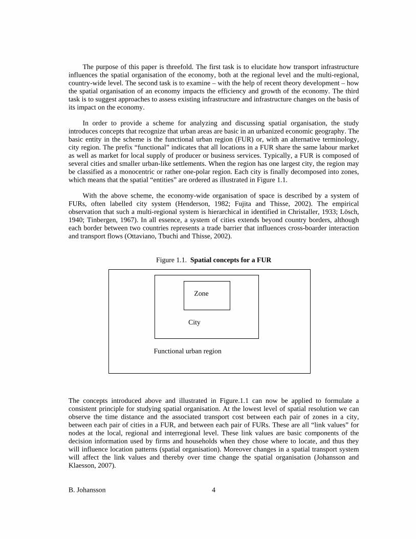
In order to provide a scheme for analyzing and discussing spatial organisation, the study introduces concepts that recognize that urban areas are basic in an urbanized economic geography. The basic entity in the scheme is the functional urban region (FUR) or, with an alternative terminology, city region. The prefix “functional” indicates that all locations in a FUR share the same labour market as well as market for local supply of producer or business services. Typically, a FUR is composed of several cities and smaller urban-like settlements. When the region has one largest city, the region may be classified as a monocentric or rather one-polar region. Each city is finally decomposed into zones, which means that the spatial “entities” are ordered as illustrated in Figure 1.1.

With the above scheme, the economy-wide organisation of space is described by a system of FURs, often labelled city system (Henderson, 1982; Fujita and Thisse, 2002). The empirical observation that such a multi-regional system is hierarchical in identified in Christaller, 1933; Lösch, 1940; Tinbergen, 1967). In all essence, a system of cities extends beyond country borders, although each border between two countries represents a trade barrier that influences cross-boarder interaction and transport flows (Ottaviano, Tbuchi and Thisse, 2002).

Figure 1.1. Spatial concepts for a FUR

The concepts introduced above and illustrated in Figure.1.1 can now be applied to formulate a consistent principle for studying spatial organisation. At the lowest level of spatial resolution we can observe the time distance and the associated transport cost between each pair of zones in a city, between each pair of cities in a FUR, and between each pair of FURs. These are all “link values” for nodes at the local, regional and interregional level. These link values are basic components of the decision information used by firms and households when they chose where to locate, and thus they will influence location patterns (spatial organisation). Moreover changes in a spatial transport system will affect the link values and thereby over time change the spatial organisation (Johansson and Klaesson, 2007).

Zone

City

Functional urban region

B. Johansson 5

1.2. Identifying infrastructure properties

The previous subsection identifies time distances between nodes or, more generally, link values reflecting generalized transport costs as a basic infrastructure property. This type of information has also been the most basic input to the established cost-benefit analysis (CBA) of infrastructure investments, which is focused on efficiency improvements. This approach has remained static in nature and focuses on marginal or piecemeal changes in transport opportunities. In Starret (1988) it is convincingly argued that CBA methods were designed to accurately solve this type of assessment problems.

In particular, welfare assessment of CBA type have especially been applied in the evaluation of investments in specific links, although there are interesting examples of approaches were changes occur in a network context (e.g. Mattsson, 1984). In a true network-based analysis the interaction flows are so-called activity based, and when this is the case, the infrastructure properties are identified and described in a way that also has an interface with emerging theories of spatial economics such as new economic geography (Krugman, 1991), agglomeration economics (Fujita and Thisse, 2002), knowledge and innovation spillover economics (Karlsson and Manduchi, 2001), new growth theory (Roemer, 1990), and new trade theory (Helpman, 1984). All these emerging strands include elements of imperfect competition, scale economies and externalities. In most cases they also imply that changes in transport costs and other geographic transaction costs matter (Johansson and Karlsson, 2001), and thus spatial organisation matters for productivity and growth – for regions and for summations across regions.

Given the above discussion, let us tentatively accept the idea that infrastructure properties impact the spatial organisation, which in turn is assumed to affect productivity as well as productivity growth. How can we then identify infrastructure properties? With reference to Lakhsmanan and Andersson (2007a, 2007b), the following alternatives should be contemplated:

(i) The capital value of infrastructure objects and the sum of such values, where the capital values are included as production factors in models that apply production, cost and profit functions to determine the infrastructure impact on the economy.

(ii) Physical or tangible properties of infrastructure objects and of infrastructure networks. Such measures include a specification of time distances, capacity, comfort and transport costs. Capacity aspects are, e.g. road length and flow capacity.

(iii) Compound measures of physical and value properties of a network, such as connectivity and accessibility of nodes to other nodes. Accessibility measures, in particular, combine link properties and features of the nodes in the network, and this provides a way to describe interaction opportunities with a vector of accessibility measures. This approach is theoretically linked to activity-based transport flow models.

1.3. Identifying infrastructure impacts on the economy and welfare

Consider that the existing transport infrastructure influences the spatial organisation and economic growth of the economy in cities and FURs. This implies that the infrastructure impact on economic development may focus on different spatial scales such as

• Consequences in individual FURs

B. Johansson 6

• Consequences in macro regions such as federal states in Germany and the USA

• Country-wide consequences

In a standard CBA approach the consequences emphasized are (i) time gains of different categories of users of the transport system, (i) reduced accident risks, reduced vehicle costs, other cost effects, including monetary value of environmental effects. A correct CBA should be based on the development network users over time, which implies that it should consider the impact of a changing spatial organisation associated with traffic system changes.

How can the effects of a changing spatial organisation of the economy be categorized? Aggregate approaches that apply production functions and dual forms such as profit and cost functions consider changes in output, productivity, and cost level. Production functions may be specified for the entire economy or for separate sectors, and they may refer to FURs, macro regions and an entire country. The idea is that an aggregate function is able to summarise micro-level effects.

In contradistinction to the production-function approach, the messages from recent developments in agglomeration economics, innovation economics and new economic geography imply that the analysis has consider the spatial organisation in a more direct way, may it by at the level of city zones, cities or FURs. The idea then is that infrastructure properties affect phenomena such as firms’ (i) labour markets, (ii) intermediary input markets, (iii) customer markets, and (iv) interaction with other firms and knowledge providers in their development activities, including R&D. These phenomena may be reflected by firms’ accessibility to labour supply, to input suppliers, to customers, and to knowledge providers. As the accessibility to input suppliers grows, increased diversity is assumed to cause augmented productivity, and as accessibility to customers improve, firms can better exploit scale economies. Changing perspective, there is also households’ accessibility to job opportunities, to supply of household services etc. The log sum of such accessibility measures may be used as welfare indicators (e.g. Mattsson, 1984)

1.4 Outline of the presentation

Section 2 outlines a framework for understanding intra-regional and extra-regional transport networks by distinguishing between local and distant markets and by classifying time distances. This forms a reference to agglomeration economies. Section 3 utilizes the framework to assess macro models that focus on the productivity impact of transport infrastructure. Section 4 presents a method to depict a region’s spatial organisation by means of infrastructure measures. This method is shown to be compatible with random choice models in trip-making models and similar transport models. Section 5 presents a set of econometric exercises with Swedish data to model and predict (i) commuter flows inside and between urban areas, (ii) growth of jobs and industries in urban areas and FURs, and (iii) interdependent evolution of labour supply and jobs in urban areas as well as for entire FURs. Section 6 concludes and suggests new directions of future research.

B. Johansson 7

2. TRANSPORT NETWORKS AND AGGLOMERATION ECONOMIES

2.1. Local and distant markets

Still in the 1970s analyses of regional economic growth relied on the so-called export-base model, according to which a region’s economy is stimulated to expand as demand from the rest of the world increases (Armstrong and Taylor, 1978). The model than predicts that service production grows in response to augmented income in the region. Already in the 1950s this perspective was modified by inter-regional input-output analyses, in models that combine intra-regional and inter-regional deliveries of goods and services (e.g. Isard, 1960).

From the beginning of the 1980s the perspective on economic growth changes in many fields of economics. New macroeconomic growth models are developed to emphasize other factors than labour and capital, and to model the growth as an endogenous process (e.g. Romer, 1986; Barro and Sala-i-Martin, 1995). These and related efforts form a background to models where public capital and infrastructure capital are included as explanatory factors in aggregate (macro) production functions. The increased focus on such phenomena also influenced the development of regional growth modeling and empirical studies.

A prime novelty in this avenue of research was the clear ambition to model economies of scale in theory-consistent way. In this atmosphere, the New Economic Geography (NEG) is developed, with models that make a clear distinction between local deliveries to customers inside a region and customers outside a region (e.g. Krugman, 1990, 1991). Other contributions emphasized agglomeration economies as a productivity and growth enhancing aspect of urban economic life (e.g. Hendersson, 1981; Fujita, 1986; Fujita and Thisse, 2002). Still another route of research focused on the innovativeness of regions, referring to the so-called Jacobs hypothesis about the role of urban diversity (Jacobs, 1969, 1984; Feldman and Audretsch, 1999). In essence, these various contributions clarify that urban economic life is distinctly different from inter-urban exchange processes, and they stress that size of urban regions matter.

Some of the conclusions drawn from the described theory development are summarized in Table 2.1, which attempts to shed light on the separation of intra-regional and extra-regional interaction and transaction. In the intra-regional context, distance-sensitive exchange and deliveries are a key feature, and require intra-urban contact networks. In contradistinction, interregional interaction and transaction is a matter for goods and service-like deliveries that have a low distance sensitivity and which may be packed and distributed in large bundles. The corresponding infrastructure networks have other features and efficiency conditions than intra-regional face-to-face (FTF) oriented interaction.

B. Johansson 8

Table 2.1. The Role of Local and Distant Markets in Economic Development

Intra-regional market phenomena Extra-regional market phenomena

Self-supporting production Production for extra-regional demand

Local markets which allow frequent FTF-contacts between buyers and sellers

Distant markets with mediated contacts between buyers and sellers and schedules delivery systems

Local competition Global competition

Infrastructure is designed to create local accessibility

Infrastructure is designed to establish accessibility in global networks

Low intra-regional transaction costs stimulate development

Low extra-regional transaction costs stimulate development

Economic growth is driven by population growth and regional enlargement

Economic growth drives population growth

Endogenous, self-generated economic growth Exogenous demand and self-generated productivity improvements stimulate economic growth

Diversity and welfare depend on the size of the region

Diversity can stimulate productivity growth and export expansion

2.2. Classifying distance sensitivity

In the subsequent presentation we consider a geography with the following structure. The basic unit is a functional region, with few exceptions a functional urban region, i.e., a FUR, which usually encompasses several cities of different size. In this sense a FUR is multicentric. However, with few exceptions one city is the largest, and the FUR is thus a one-polar region. For each city we will consider a set of zones and a set of links which make the city as well as the region as a whole a network of transport links and activity nodes, hosting residential buildings and firm premises.

Consider two zones (nodes in urban areas), labelled k and l, and let the time distance on the link

(k, l) be klt . Such link distances may be associated with several alternative transport modes, and then we could specify mode-specific time distances for each link. For the moment we shall only consider one time distance value for each link. Before proceeding, it should be stressed that the importance to a city of a link (k, l) depends on characteristics of node k and node l, such as the number of node inhabitants, the number of jobs, the size and diversity of service supply for household and for firms.

Referring to Swedish data, which according to the literature seem fairly representative, time distances can be divided into local (intra-city), regional (intra-regional) and interregional (extra-regional) as specified in Table 2.2

B. Johansson 9

Table 2.2. Classification of time distances between zones

Time interval in minutes Average travel time in minutes

Between zones in the same city (local) 0 - 15 8 - 12

From a zone in a city to zones in other part of the FUR (regional)

15 - 50 25 - 35

From a city in a FUR to a city in another FUR (inter-regional)

More than 60 More than 60

From Table 2.2 we can make several observations. The first has to do with sparsely populated land between cities and hence also such land between FURs. If a country’s area is divided into exhaustive and mutually exclusive FUR areas, some parts of the geography will not match the time specifications in the table. However, from a transport point of view flows on links to such places are so thin (or infrequent) that they statistically will have close to measure zero, and hence can be disregarded for all practical purposes.

The second observation is that the separation between intra-regional and extra-regional links has an empty interval, from 50 to 60 minutes. Again, that reflects that FURs or city regions normally are sufficiently far away from each other to be divided by “empty land”, just as mentioned above.

As a third observation we note that Table 2.2 provides an implicit definition of a FUR. It is a functional area, for which the time distance between any (or most) pairs of zones is shorter than 50 minutes. From this point of view a FUR allows firms and households to have frequent contacts with suppliers of household and producer or business services. In this way the city region is also an arena for knowledge interaction and diffusion. Moreover, the FUR can be an integrated labour market area. In addition, each city itself is an arena for very frequent face-to-face interaction, although it is only the largest cities in region that host sufficiently many actors to offer frequent interaction opportunities.

There is a final aspect of Table 2.2 that should be discussed. The model suggestions in sections 4 and 5 are twofold. First, as time distances are reduced an increasing share of all deliveries are not planned or scheduled in advance, but can take place on short notice. For long time distances the opposite holds and they will therefore generally be associated with more logistic-systems arrangements, like large shipments, multipurpose trips, supply-chain optimisation and the like. Second, theoretical development of the economics of agglomeration tells us that activities with frequent interaction have an incentive to cluster in the neighbourhood of each other.

We may also remark that a measure of time distances incorporate both economies and diseconomies of density. When an urban area becomes too dense of activities and interaction, congestion phenomena emerge and time distances will rise. New infrastructure networks may again remedy this type of development.

B. Johansson 10

3. TRANSPORT INFRASTRUCTURE AND NEW GROWTH THEORY

3.1. Endogenous growth and growth accounting

Transport infrastructure affects options to interact inside and between regions, and in this way it influences economic efficiency. We may then ask: does improved efficiency imply anything about regional economic growth? In a strict neoclassical setting, there is no direct link between efficiency and growth. A step towards a link between infrastructure and economic growth is present in Mera (1973), where public infrastructure influences productivity. During the 1980s we can identify a sequence of studies applying national and regional production and cost functions, where infrastructure is a factor of production (e.g. Wigren, 1984; Elhance and Lakshmanan, 1988; Deno, 1988). The discussion of the productivity impact of infrastructure was strongly intensified by several papers by Aschauer (1989, 2000).

The attempts to model and estimate the role of transport infrastructure may be classified into two avenues. Along the first, transport infrastructure is represented by capital value, as one form of public capital, and thus relates to the general question: Is public capital productive? Two typical studies of this kind can be found in Aschauer (1989) with an aggregate production-function model of the US economy, and in Aschauer (2000) with an aggregate model specified for a set of macro regions.

The second avenue is to measure transport infrastructure in terms of its “physical” attributes, an approach that primarily is applied to regional cross-sectional or panel data from at set of regions. With this approach transport infrastructure may be represented by a variable like highway density or degree of agglomeration (e.g. Moomaw and Williams, 1992; Carlino and Voith, 1992).

The two approaches to assess the productivity and growth effects of infrastructure capital differ in a fundamental way. Infrastructure capital is a one-dimensional measure, and such a measure should be expected to fail when applied to different investments or different regions. A kilometre highway that solves exactly the same way in two different regions should have the same effect in both regions. However, if it is much more expensive to construct the road in the first region, the capital value would be higher in this region and, as a consequence; the output elasticity of a kilometre highway would differ between the regions. With a physical measure this problem disappears.

A similar issue is the option to describe transport-infrastructure capital with a vector instead of a single value, where each component refers to a specific type of transport capital, such as road, rail, air terminals, etc.

If capital values are used for large regions or for an entire country, the above problems could be expected to disappear with the help of the law of large numbers. We may also observe the following pattern:

• Time series econometrics for countries tend to use an aggregate capital value of transport infrastructure

B. Johansson 11

• Cross-regional and panel-data econometrics tend to use physical attributes of transport infrastructure

What is then the theoretical framework of the aggregate country-wide analyses of the role of transport infrastructure in economic growth? From one point of view they adhere to the idea behind endogenous growth. However, the studies contain very little of explicit references to endogenous growth, although the approach most likely would benefit from examining such model formulations. For one thing, infrastructure capital is to some extent public in the same way as knowledge in the core model of endogenous growth. In spite of this the studies referred primarily have the form of growth accounting.

Another issue in these studies is the choice of estimating a production function or a cost function for the economy or for a set of different sectors. Examples of studies using a cost-function approach are Seitz (1993) and Nadiri and Mamanueas (1991, 1996). What are then the advantages of a cost-function (or profit function) approach? In brief, a cost function estimation has direct support from microeconomic theory, because

• The estimation is based on optimization assumptions

• Duality conditions such as Shephard’s lemma allows for controlled conclusions

• The approach makes it possible to distinguish between variable and fixed costs

• The approach makes it possible to consider scale economies

• The estimation considers how both supply and demand adjustments influence productivity growth

• The approach comprise not only capital and labour inputs, but also intermediary inputs

3.2. Assessing dissonant results

In Lakshmanan and Anderson (2007) it is observed that the whole range of studies that examine the productivity of infrastructure have generated quite dissonant estimates of output and cost elasticities. These results differ sharply for the same country, for countries at comparable stages of development and for countries at different stages of development. In view of this they pose the question: Is macroeconomic modeling of transport infrastructure unable to incorporate key transport-economy linkages? In this context they point at several problems such as (i) the network character of roads and other transport modes, (ii) threshold phenomena in transport development, (iii) the state of the pre-existing transport network, (iv) the state of development in regions undergoing transport improvements, (v) the structure of markets in regions, (vi) the presence of spatial agglomeration economies, and (vii) the potential for innovation economies.

Lakshmanan and Andersson (2007) discuss what they call the traditional view that transport infrastructure contributes to economic growth and productivity. In this discussion they emphasize that a set of recent methodologically sophisticated studies produce markedly dissonant estimates of the productivity of transport infrastructure, where the return to transport capital varies in a disturbing way. In the subsequent presentation it claimed that one reason for the lack of consistency between those empirical efforts is related to how transport infrastructure is identified and measured.

B. Johansson 12

The measurement and definition of transport infrastructure involves a set of partly interrelated choices such as

• A compound measure of transport infrastructure versus a vector specifying different types of infrastructure

• National versus regional specifications of available transport infrastructure

• The capital value of transport infrastructure versus physical and systems properties of the infrastructure

The options above can be included in alternative econometric approaches. For example, some studies apply cross-section analysis, whereas others employ time-series analyses. Moreover, the cross-section choice comprises the option to distinguish between industries (sectors of the economy), as well as multi-regional information. Combining these different observations the options of econometric approaches can be specified as illustrated in Figure 3.1

Figure 3.1. Overview of approaches to estimate infrastructure productivity

Time-series, cross-section and panel data analysis all allow a choice between measuring (i) physical attributes and (ii) pecuniary values of infrastructure. The initial studies of infrastructure productivity were applying time-series analysis with an aggregate capital value and using GDP as the dependent variable. Naturally, the result from such studies can only be useful decision support for macroeconomic problems, such as the typical Aschauer questions: Is public expenditure productive or Do states optimize? Estimated elasticities are not useful for individual investment decisions for the following reasons:

Econometric approaches

Cross-section analysis • Multi-sector

information • Multi-regional

information

Panel data Combined time-series and cross-sectional analysis

Time-series analysis for one sector and one region

Physical measures of infrastructure properties • Summarizing across

transport systems • Different types of

infrastructure

Pecuniary measure like capital value • Aggregate value for the

entire transport system • Different types of

infrastructure

B. Johansson 13

• Two different highway projects that generate the same “amount of transport services” may differ in cost by factor 2 or 3. Thus, capital values are not correlated with the amount of service. This argument is weakened in the aggregate due to the law of large numbers.

• If the value of different types of infrastructure like roads, railway and air terminal are aggregated together results will be ambiguous. Instead a vector with capital value components referring to different types of infrastructure may reveal system composition or substitution effects. Again, the acquired result will be relevant only for an “average investment project”.

The second alternative is labeled “physical measure”. Obviously, such measures must be collected at a disaggregate level, with information from regions, in particular FUR-level data. However, first we have to clarify what is meant by “physical attributes. For roads, one may use variables such as (i) kilometer highway per regional area, (ii) flow capacity per regional area, (iii) time distances to neighbouring metropolitan regions, (iv) time distances to terminals for international freight. Measures of this kind can be applied in regional system models as demonstrated by followers of Mera, such as Sasaki, Kunihisa and Sugiyama (1995), and Kobayashi and Okumura (1997). They estimate relations between production, transport deliveries for regions and apply these estimates in multi-regional models with consistency constraints for each region and for the multi-regional system as a whole. This type of model is then used as a means to predict effects on the system of changes in the infrastructure in one or several regions. This approach has a clear interface with so-called activity-based models for transport forecast, and it captures the fact that regional context matters.

Another way to reflect physical attributes of a transport infrastructure is to calculate how it affects time distances between nodes in a transport network. Improved road and railroad infrastructure quality can reduce such time distances. This measure will also indirectly reflect capacity, since insufficient capacity will cause time delays (congestion) and thereby reduce speed, which implies that time distances increase. In Section 4 we will demonstrate how time distance information about transport infrastructure can be combined with information about activities in the nodes of the infrastructure network to yield purposeful characterization of infrastructure networks. Information about time distances and activity location is combined into accessibility measures.

3.3. Productivity impacts of infrastructure measured by physical attributes

Spatially aggregated models are not designed to reflect how and why transport infrastructure can have different effects on productivity in different regions. The impact of additional infrastructure may be weaker in a region which is already infrastructure affluent than in other regions with less developed infrastructure. The effects could also be greater in dense metropolitan regions than elsewhere. However, we also know that when a smaller region gets shorter time distances to a larger region, then the income may increase for the smaller region. In addition, such regional integration implies that the larger region increases its market potential, which should imply higher productivity in view of models of agglomeration economies and new economic geography (NEG)

A major conclusion is that aggregate models provide information that is macro relevant, by estimating effects which reflect consequences attributed to “an average bundle of infrastructure objects or to an average infrastructure investment project. The meaningfulness of estimates has to rely on the law of large numbers. The same conclusion applies with regard to using GDP as dependent variable contra using sector-specific output values.

B. Johansson 14

The way to avoid the problems addressed is two-fold. First and foremost, when the infrastructure is recorded in terms its attributes instead of capital values, then econometric exercises will reflect effects that have an interface with effects that are included in orthodox CBA evaluations. Second, cross-regional observations give rise to enough variation for more reliable results that are also open for more insightful interpretations. A third possibility is to employ panel data.

With the suggested approach one may consider three major issues:

• How does infrastructure attributes stimulate structural changes in the economy, with exit and entry of activities?

• Will a region’s output rise or fall? How fast is the change of GRP?

• What happens with a regions productivity in terms of GRP or income per capita?

In Table 3.1 a set of regression results are presented. They are all based on cross-regional information. In addition, all studies – except the Merriman study – use information about infrastructure attributes. As a consequence we can observe that productivity impacts vary considerable between regions.

Table 3.1. Regional productivity impacts from physical attributes of transport infrastructure

in regional cross-section analysis

Researcher Estimation results

Andersson et.al. (1990) Large productivity effects which vary considerably between regions

Anderstig (1991) The rate of return to an investment varies with regard to in which region the investment takes place, generating examples with both high and low returns

Wigren (1984, 1985) Considerable productivity effects which vary in size between regions

Sasaki et.al. (1995) Considerable productivity effects that vary markedly between regions

Bergman (1996) Productivity effects vary strongly between regions of different size. Considers both intra-regional and inter-regional infrastructure networks

Merriman (1990)* Considerable effects

* The study by Merriman does not employ physical measures of infrastructure attributes.

Table 3.2 contains studies that employ panel data, with regional specification for a sequence of dates or just for a start year and a final year. Three of the studies use infrastructure attributes as explanatory variables, and these may be considered as panel data variants of the studies in Table 3.1. All studies in the table report that productivity effects and rate of return to investments vary strongly between regions.

B. Johansson 15

Table 3.2. Regional productivity impacts from transport infrastructure in panel data estimations, with physical infrastructure attributes in three cases

Researcher Estimation results

Carlino and Voith (1992)

Large productivity effects of (i) highway density and (ii) agglomeration level

Johansson (1993) Rate of return to an investment varies across regions and hence attains both high and low values. Effects of both intra-regional and inter-regional infrastructure networks

Mera (1973a, 1973b) Productivity effects differ considerably with regard to region of investment

Seitz (1995)* Rate of return to an investment varies across urban regions and hence attains both high and low values.

McGuire (1995) Clear productivity effects that vary between regions

Table 3.2 presents examples of estimations that (i) use panel-data information and (ii) information about infrastructure attributes. An overall observation is that these estimations tend be robust with regard to variation in parameter values. Together with ordinary cross-regional studies they produce lower parameter values than aggregate production function specifications. This is the background to the conclusion that they are more reliable. Does this mean that they can replace CBA approaches? The conclusion that we will arrive at later is that they are rather complements than substitutes.

4. NETWORKS AND ACCESSIBILITY

4.1. Spatial organisation and accessibility

The previous section observes that the production function (or cost function) approach capture urban and other density and collocation externalities in a crude and indirect way. At the same time we clarified that modern spatial economics modelling promotes such externalities as important and use them as necessary to explain the very existence of cities and city regions.

Section 2 introduces time distances between nodes (zones) in regions as an important aspect of a region’s spatial organisation. In the present subsection we start with these distances and add information about activities in each node to get full picture of the spatial organisation. Referring back to Figure 1.1 we can observe that a one-polar FUR consists of a major city (central city) together with other neighbouring cities and urban areas, where “city” is included in the notion “urban area”. Each city and urban area consists of zones, and the region’s transport system is reflected by the time

B. Johansson 16

distances between al zones. Reducing the dimensionality of such a time-distance matrix, we can focus on the following “aggregate” time distances:

(i) Intra-urban: The average time distance between all nodes in a city (urban area), denoted by kkt for urban area k.

(ii) Intra-regional: The average time distance between urban area k and l inside region R,

denoted by klt , for )(kRl ∈ , where )(kR is the set of urban areas that belong to the same FUR as k, except k itself.

(iii) Extra-regional: The average time distance between urban area k in region R and urban area l

outside region R, denoted by klt , for lk ≠ and )(kEl ∈ , where )(kE is the set of urban areas that do not belong to the same FUR as k.

Next, consider that we can collect information about the number of jobs in each urban area k,

denoted by kJ . Then we can select another urban area s and make the following calculations for a household with residence in s:

The accessibility to jobs in s equals { }sssssJ

ss JttT )(exp λ−= (4.1a)

The accessibility to jobs in )(sR equals { }∑ ∈−=

)()( )(expsRk ssksk

JsR JttT λ

(4.1b)

The accessibility to jobs in )(sE equals { }∑ ∈−=

)()( )(expsRk ssksk

JsR JttT λ

(4.1c)

Two properties of the formulas in (4.1) need comments. The first is that the time-sensitivity parameter λ is modelled as a function of the actual time distance. The reason for this is that empirical studies with Swedish data strongly suggest that the time sensitivity for short, intermediate and long distances are different (Johansson, Klaesson and Olsson, 2002, 2003). The second observation is that the three accessibility measures are determined only by time distances and job location. One might

argue that the value )( sksk tλλλ == should reflect generalized transport costs. As shown in the following subsection, an estimation of λ will reflect time costs and other trip costs accurately if these two components both are proportional to time distance.

The basic message now is that the vector [ ]JsE

JsR

Jss TTT )()( ,, provides us with one description of the

spatial organisation of a region from the perspective of an urban area (city) s in region R. As we shall see, this is just one out of several such descriptions that will be suggested. Before any further step is taken, two basic changes in the spatial organisation will be illustrated. As the first type of change,

consider that the number of jobs in urban area k increases from kJ to kk JJ Δ+ . The resulting change in the accessibility to jobs on link (s, k) is calculated in (4.2a)

{ } kskskJ

sk JtT Δ−=Δ λexp (4.2a)

B. Johansson 17

The second type of change is generated by a change in the time distance skt . Suppose that the

distance increases by sktΔ . This will result in the following reduction of job accessibility on link (s, k):

{ } { }[ ] ksksksksk Jtt Δ−−− λλ exp1(exp (4.2b)

Returning to formula (4.1), it should be observed that we can shift from the location variable sJ

to a variable showing the labour supply from households in s, denoted by sL , to a variable referring to

the supply of business services, denotes by sF , or to a variable informing about the supply of

household services, denoted by sH . Applying the technique in formula (4.1), this would allow us to characterize an urban area s in the following complementing ways:

A household’s accessibility to jobs, depicted by the vector =JsT [ ]J

sEJ

sRJ

ss TTT )()( ,, , and to

household services, given by the vector =HsT [ ]H

sEH

sRH

ss TTT )()( ,, . (4.3a)

A firm’s accessibility to labour supply, depicted by the vector =LsT [ ]L

sEL

sRL

ss TTT )()( ,, , and to

business services, given by the vector =FsT [ ]F

sEF

sRF

ss TTT )()( ,, . (4.3b)

The accessibility measures calculated in this way evidently reflect interaction and contact opportunities of households and firms, respectively. Classical references would be Lakshmanan and Hansen (1965, and Weibull (1976). If we introduce a variable that can represent customer budgets in different locations, it is also possible to calculate sales and delivery opportunities.

The second requirement for the accessibility measures is that they should be compatible or consistent with models designed to predict trip making and transport flows. This issue is illustrated for labour-market commuting in the next subsection.

4.2. Job accessibility, random choice and commuting

Consider now a set of urban areas (cities and towns) belonging to the same FUR Rk ∈ . For

urban area k, kL is the potential labour supply and kM ≤ kL is the realized labour supply at any point in time. This means that supply is recognized as all persons in place k who live there and have a job in the same place or somewhere else. For the same group of urban areas we can also identify the number

of available jobs in each municipality k, denoted by kJ . Commuting from area k to area l is denoted

by klm such that

kkll Mm =∑ , and lklk Jm =∑ (4.4)

B. Johansson 18

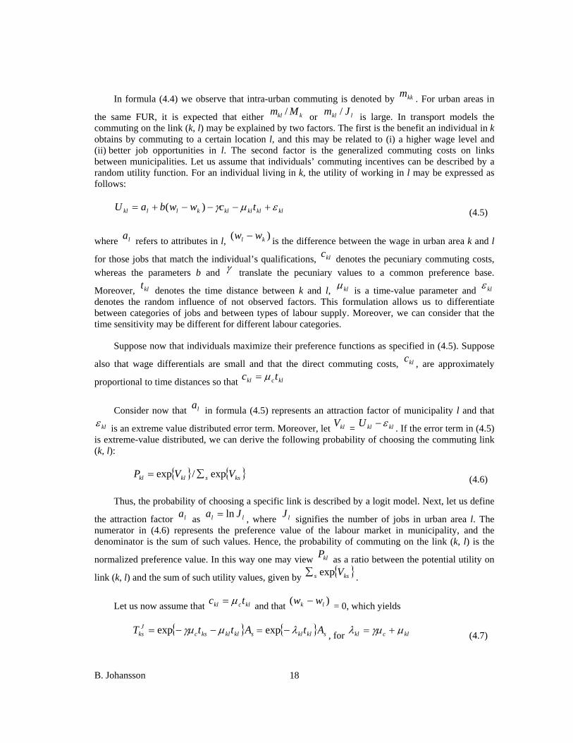
In formula (4.4) we observe that intra-urban commuting is denoted by kkm . For urban areas in

the same FUR, it is expected that either kkl Mm / or lkl Jm / is large. In transport models the commuting on the link (k, l) may be explained by two factors. The first is the benefit an individual in k obtains by commuting to a certain location l, and this may be related to (i) a higher wage level and (ii) better job opportunities in l. The second factor is the generalized commuting costs on links between municipalities. Let us assume that individuals’ commuting incentives can be described by a random utility function. For an individual living in k, the utility of working in l may be expressed as follows:

klklklklkllkl tcwwbaU εμγ +−−−+= )( (4.5)

where la refers to attributes in l, )( kl ww − is the difference between the wage in urban area k and l

for those jobs that match the individual’s qualifications, klc denotes the pecuniary commuting costs, whereas the parameters b and γ translate the pecuniary values to a common preference base.

Moreover, klt denotes the time distance between k and l, klμ is a time-value parameter and klε denotes the random influence of not observed factors. This formulation allows us to differentiate between categories of jobs and between types of labour supply. Moreover, we can consider that the time sensitivity may be different for different labour categories.

Suppose now that individuals maximize their preference functions as specified in (4.5). Suppose

also that wage differentials are small and that the direct commuting costs, klc , are approximately

proportional to time distances so that klckl tc μ=

Consider now that la in formula (4.5) represents an attraction factor of municipality l and that klε is an extreme value distributed error term. Moreover, let klV = klklU ε− . If the error term in (4.5)

is extreme-value distributed, we can derive the following probability of choosing the commuting link (k, l):

{ } { }kssklkl VVP exp/exp ∑= (4.6)

Thus, the probability of choosing a specific link is described by a logit model. Next, let us define

the attraction factor la as ll Ja ln= , where lJ signifies the number of jobs in urban area l. The numerator in (4.6) represents the preference value of the labour market in municipality, and the denominator is the sum of such values. Hence, the probability of commuting on the link (k, l) is the

normalized preference value. In this way one may view klP as a ratio between the potential utility on

link (k, l) and the sum of such utility values, given by { }kss Vexp∑ .

Let us now assume that klckl tc μ= and that )( lk ww − = 0, which yields

{ } sklklkscJ

ks AttT μγμ −−= exp { } sklkl Atλ−= exp , for klckl μγμλ += (4.7)

B. Johansson 19

which is the standard measure of job accessibility on a link (k, l) introduced in the preceding subsection. It provides an exact measure only if the assumption about equal wages is valid. We should

also observe that the new time-sensitivity parameter klλ = )( klc μγμ + .

Given the exercises above, how do the accessibility measures relate to predictions of transport (commuter) flows? To see this, consider the expression in (4.6). From this we can predict the number

of commuter trips between k and l as klm = { } { }kssklk VVM exp/exp ∑ , where { }klVexp = J

klT , and where the denominator is a normalizing factor, based on the sum of all link accessibilities originating from urban area k. Moreover, it is also possible to include other attractiveness factor in the

specification of ksV , that may distinguish between intra-urban, intra-regional and extra-regional flows as shown in Johansson, Klaesson and Olsson (2003). This approach provides empirical model results

which reveal that the time sensitivity parameter (variable) )( klkl tλλ = is a non-linear function of klt ,

represented by three different values such that okk λλ = , 1λλ =ks for )(sRs∈ and 2λλ =ks for )(sEs∈ , as presented in Table 4.1.

Table 4.1. Nonlinear commuter response to time distance

Intra-urban commuting Inter-regional commuting

Extra-regional

Time distance klt 0- 15 minutes 15-50 minutes More than 60 minutes

Time sensitivity klλ oλ is very low 1λ 18.3 λ≈ oλλ 1.22 ≈

Additional destination preference

Strong preference for local commuting

Medium preference for regional commuting

No preference

Source: Johansson, Klaesson and Olsson (2003).

The properties presented in Table 4.1 refer factors that can be included in an accessibility

measure, and hence add to the possibility to reflect the spatial organisation of a FUR.

4.3. Different ways to make use of accessibility measures

The previous presentation attempts to illuminate how a region’s spatial organisation can be revealed by means of accessibility measures. The presentation aims at making precise how these measures change (i) as firms (jobs) and households (labour supply) migrate into or out from urban areas in a region, and (ii) as time distances change inside each urban area and between different areas. However, it remains to discuss how accessibility measures can be employed in the assessment of transport infrastructure policies.

B. Johansson 20

First, let us consider the set of accessibility measures presented in Table 4.2. The table presents an overview of alternative measures and the processes and consequences associated with each measure.

Table 4.2. Overview of optional accessibility measures

TYPES OF ACCESSIBILITY ASSOCIATED PROCESSES AND CONSEQUENCES

HOUSEHOLDS’ ACCESSIBILITY TO Jobs In terms of dynamics, households are attracted to

locate in places with high accessibility to jobs. In terms of efficiency, high accessibility implies better labour-market matching

Household services Households are attracted to locate in towns and cities with high accessibility to services, as well as diversity of services

Wage sum in firms located in different areas Households are attracted to locate in towns and cities with high accessibility to economic activities, that may reflect job diversity, higher than average wages and productivity

FIRMS’ ACCESSIBILITY TO Labour supply In terms of dynamics, firms are attracted to places

with high accessibility to labour supply. In terms of efficiency, high accessibility implies better labour-market matching

Knowledge intensive labour supply Growing economic sectors are oriented towards knowledge-intensive advanced services. Accessibility to a matching labour supply attracts firms belonging to growth sectors

Wage sum of households residing in different areas

Reflects the size of market demand for firms supplying household services; with an expanding local market scale economies can be exploited and diversity can increase

Wage sum in firms located in different areas Reflects the size of market demand for firms supplying business (producer) services; with an expanding local market scale economies can be exploited and diversity can increase

With information of the type illustrated in Table 4.2, it is possible to consider at least four areas where the accessibility measures can be applied. These areas will be treated under the following labels:

B. Johansson 21

• Prediction of flows. Accessibility to household services could for example be used to predict shopping trips but also migration flows. In section 5 empirical results are provided for commuting to work. Obviously, such predictions should be an important subtask in CBA calculations.

• Prediction of location patterns. Accessibility to labour supply can be used predict changes in the number of jobs in different parts of a FUR, and thus in the entire FUR. In an analogous way, the size of labour supply may be predicted. Observe that if jobs and labour supply increases in a region, this should potentially generate additional agglomeration effects, with productivity implications. In addition, changes in job location can indeed be carried out for specific groups of sectors.

• Prediction of economic change. With similar approaches as for prediction of location patterns, the growth and decline in employment and output (value added) can be predicted for a FUR. Such predictions can also focus on groups of sectors like private services, business services, etc.

• Prediction based on output elasticities. In this case FUR-specific accessibility measures are used as indicators of the services provided by transport infrastructure. This opportunity would, for example, fit a cross-regional version of the cost-function and total factor-productivity analyses by Nadiri and Manueas (1996).

The fundamental idea behind the four suggestions above is that accessibility measures are assumed to reflect the potential services that a region’s internal and external transport infrastructure networks afford. If they offer such services, as claimed in this presentation, then it should be possible to estimate relations for both level and growth specifications, based on cross-region and panel data specifications, respectively. Moreover, accessibility measure should emerge as significant inputs in production function formulations. This latter opportunity may also take the form cost-function formulations of the type employed by Nadiri and Mamuneas (1996).

Let us first consider the fourth option, labeled output elasticity estimation. This may take the form of estimating production functions with cross-regional information with FURs as observation units. Since some FURs have limited size, this also implies a restrictive sector specification. It also implies that accessibility measures have to be calculated as averages for each FUR. Each FUR, signified by R, could then be represented by the following three-component:

ssRs

sI

R TgT ∑∈

= , ∑∈

=Rs

sg 1

∑∈

=Rs

sRsII

R ThT )(, ∑∈

=Rs

sh 1 (4.8)

∑∈

=Rs

sEsIII

R TqT )(, ∑∈

=Rs

sq 1

where sg , sh and sq are weighting factors. The T-variables in (4.8) as separate observations of a region’s transport system, and each T-value could represent local, regional and extra-regional accessibility GRP (gross regional product or wage sum) of each FUR. Other options are accessibility

B. Johansson 22

to port capacity (Johansson, 1993), airport capacity Andersson, Anderstig and Hårsman, 1990) or knowledge resources (Andersson and Karlsson, 2005).

In order to predict location patterns one might consider cross-section estimations generating information about location pattern and accessibility structure in terms of levels. However, it may be more rewarding to consider estimations of change processes, such that the change of, for example, jobs in urban areas is regressed against the accessibility pattern for each urban area at the start year. This approach comes close to the so-called Carlino-Mills model (Mills and Carlino, 1989).

This paper argues that the spatial organisation of a FUR can be described by a FUR-vector =RT [ ]III

RII

RI

R TTT ,, , and by vectors [ ]IsEsRss TTT )()( ,, for each urban area s. Are there any other

structural aspect that adds important information about the spatial organisation? The empirical results in Section 5 indicate convincingly that additional insights can be gained by incorporating the Christaller conjecture about a hierarchical pattern, known as the central-place system (CPS) model. In view of this, the following arrangement of urban areas is suggested, with three groups of urban areas, labeled C1, C2, and C3, where

C1 = The central and largest city in each region

C2 = Other urban areas in large FURs (more than 100 000 inhabitants) (4.9)

C3 = Other urban areas in small FURs (less than 100 000 inhabitants)

It is possible to make use of the CPS idea by estimating model parameters in a separate regression equation (or equation system) for each category of urban areas, while still using measures of accessibility to all types of urban areas.

Consider now that there is a prediction of job changes for each urban area in a FUR. Then the total effect for the FUR is assumed to be the sum of the change in each of the individual areas. Suppose now that the total number of jobs has increased. Is this growth an addition to the entire economy, across different FURs. The suggestion here is that it is an addition, in line with models of agglomeration economies. Thus, the number of jobs is not governed by zero-sum game restrictions.

There are empirical observations supporting the conclusion above. First, when using accessibility measure to explain (or predict) growth in FURs, one can observe that not all FURs have a positive growth. Second, empirical observations for the last two decades in Sweden tell us the following:

• The labour productivity as reflected by the wage level is positively correlated with an urban area’s accessibility to jobs, to labour supply and to the wage sum.

• The labour market participation rate is positively correlated with an urban area’s accessibility to jobs, to labour supply and to the wage sum.

These two observations support the assumption that accessibility properties have productivity effects.

B. Johansson 23

5. EMPIRICAL RESULTS FROM ACCESSIBILITY-BASED STUDIES

5.1. Commuting and the spatial organisation of a FUR

Commuting can be viewed as a by-product of the spatial organisation of a FUR, and reflecting forces which are striving to equilibrate the supply of labour and the demand for labour. Viewing the labour market in this way makes it natural to relate commuting to spatially separate locations where supply in one location meets demand in another. In this context, the aim of this subsection is to illustrate how well measures of labour-market accessibility can depict the spatial organisation and the corresponding commuter flows. This accomplished by means of two equations with the following structure (Johansson, Klaesson and Olssson, 2002):

• Commuting into an urban area is positively affected by (i) the intra-urban accessibility to jobs, and by (ii) the area’s accessibility to labour supply in neighbouring (surrounding) urban areas.

• Commuting out of an urban area is positively affected by (i) intra-urban accessibility to residents in the area who have a job somewhere, and by (ii) the area’s accessibility to jobs in neighbouring urban areas.

Following the structure above we make use of two accessibility measures for in-commuting to

area k, denoted by kI . The first measure is the job accessibility in k, J

kkT , and the second is =L

RET LkE

LkR TT )()( + , which summarizes the entire accessibility to labour supply outside the urban area.

This yields the regression equation

kL

REJ

kkk TTI εγβα +++= (5.1)

The results of the regressions for 1990 and 1998 are shown in Table 5.1. All slope coefficients are positive and highly significant. In particular, we observe that most of the variation is captured by the two-variable equation.

Table 5.1. Commuting into municipalities 1990 and 1998

1990 1998 Intercept, α -3374.2 (-6.3) -2780.6 (-6.3)

Internal accessibility to jobs, β 0.37 (41.6) 0.39 (49.1)

External accessibility to realized labour supply, γ

0.05 (5.4) 0.06 (6.5)

2R adj 0.94 0.95

Remark: t-values are shown within parentheses. Number of observations is 288.

B. Johansson 24

It should be observed that equation (5.1) provides a measure of each inter-urban flow, because L

RETγ is the sum of link-specific elements like { } kklkl Ltλ−exp .

The regression equation for out-commuters is described in (5.2). The two explanatory variables

are L

kkT and J

RET , denoting intra-urban accessibility to residents in the area who have a job somewhere and the area’s accessibility to jobs in neighbouring urban areas, respectively. The dependent variable,

kO , denotes the total out-commuting from urban area k.

JRE

Lkkk TTO γβα ++= (5.2)

where Ok denotes out-commuting from municipality k, L

kkT denotes the internal accessibility to realized

labour supply, and J

RET denotes the external accessibility to jobs outside the urban area k. The results of estimating equation (5.2) for 1990 and 1998 are displayed in Table 5.2. All slope coefficients are positive and highly significant, and a large portion of the variation is explained by the two independent accessibility variables.

Table 5.2. Commuting out of municipalities 1990 and 1998

1990 1998

Intercept, α -291.1 (-6.3) -237.9 (-0.9)

Internal accessibility to realized labour supply, β

0.15 (41.6) 0.18 (28.2)

External accessibility to jobs, γ 0.07 (15.0) 0.07 (16.0)

2R adj 0.93 0.95

Remark: t-values are shown within parentheses. Number of observations is 288.

Tables 5.1 and 5.2, taken together, illustrate the strong correspondence between the spatial organisation of a FUR and the commuter transport flows. It may also be remarked that the time distances employed in the regression of (5.1) and (5.2) refer to commuting by car, which is the overwhelmingly dominating mode in all FURs except in the Stockholm region, for which automobile commuting still dominates but with a considerable share of public-transport commuting.

B. Johansson 25

5.2. Sector development in cities and regions

The economics of agglomeration is a field of models that focus on activities that may cluster in space to allow for distance-sensitive interaction. As presented in Fujita and Thisse (2002) these types of interaction include information and knowledge exchange between firms, and distance-sensitive contacts between supplier and customers. In dynamic context, the economies of scale may also be related to the so-called home-market effect in models classified as new economic geography.

This subsection presents models which reflect agglomeration economies with each urban area’s accessibility to the wage sum in the area itself and in other parts of the FUR, to which the area belongs. The wage sum corresponds to a large share of each city’s and town’s total value added

For each urban area s, the accessibility to wage sum is expressed by a vector =WsT [ ]W

sRW

ss TT )(, , which only consists of intra-urban and intra-regional accessibility. The reason for excluding the extra-regional accessibility has a statistically insignificant and minimal influence on the change processes examined here. The very straightforward approach is formulate a simple growth equation for jobs, supply of household services, and supply of business services as described in (5.3). The two service-supply variables are reflected by the number of jobs in the pertinent industries. Having said this, one could observe that job growth during the 1990s (and later) is primarily a growth of jobs in private services.

sW

sRW

ssos TTJ εααα +++=Δ )(21

sW

sRWssos TTH εααα +++=Δ )(21 (5.3)

sW

sRW

ssos TTF εααα +++=Δ )(21

where the first equation refers to change of all jobs, the second to the change persons employed in household service industries, and the third to the change of persons employed in business service industries.

Table 5.3 . Growth 1993-2000 in central cities induced by the accessibility to wage sum1993

CHANGE PROCESS oα 1α 3α

2R

sJΔ Growth of jobs -684

(-4.4)

0.58 (8.7)

0.75 (2.1)

0.97

sHΔ Growth of household service supply -425

(-3.4)

0.42

(7.8)

0.64

(2.2)

0.97

sFΔ Growth of business service supply -939

(4.3)

0.95

(10.2)

1.31

(2.7)

0.98

B. Johansson 26

Table 5.3 presents results for the central (largest) city in each FUR. Similar regressions for non-central cities and towns shows that a similar pattern but with somewhat lower

2R -values for C2-areas, and much lower for C3-areas. For the latter group, the regression results imply that the estimated equation has a low prediction accuracy. In all essence, this reflect that service supply in Sweden is concentrated in the central city of each FUR and that this also implies that overall employment growth is strongly associated with the central cities, because overall growth is driven by service sector growth. For the three metropolitan FURs, this observation is less accentuated, which means that metropolitan growth is shared between the C1-area and the C2-areas.

It should be stressed that the models in (5.3), the accessibility measures are given for the start year, and growth is the result of a given spatial organisation at the start year. This means that different FURs can be compared and assessed with regard to their inherent change qualities. How is then assessment of planned infrastructure investments and other network changes carried out? The strategy for this is simple. First the growth path (change process) with the given accessibility pattern is calculated. In a second step the growth path associated with a new accessibility structure is calculated. The consequence of infrastructure changes is then the differences between the first and the second growth path.

5.3. FUR growth and interdependencies in the spatial organisation

In this and the following subsection the focus is on the labour market, with reference to a model presented in Johansson and Klaesson (2007). This model assumes (i) that labour supply (households) is attracted to an urban area in response to the area’s accessibility to jobs, and (ii) that jobs (firms) are attracted to an urban area in response to the area’s accessibility to labour supply. Such change processes operate also when the infrastructure properties remain unchanged, but will change as accessibility patterns are altered. It should be emphasized that the two change processes introduced constitute “coupled dynamics”, and the initial task is to clarify these dynamics.

The dynamics on the labour market will be specified for each urban area, m. The supply of labour

is depicted by the accessibility vector ],,[ )()(L

mEL

mRL

mm TTT as specified in (4.3), and labeled urban area m’s accessibility to labour supply. The demand for labour is reflected by the accessibility vector

],,[ )()(J

mEJ

mRJ

mm TTT as specified in (4.3), and labeled area m’s accessibility to jobs. The two vectors are dynamically related through the two equations in (5.4a) and (5.xb), specified as follows for each of the three groups of municipalities, C1, C2 and C3, which are introduced earlier in (4.9):

),,( )()(L

mEL

mRL

mmm TTTfJ =Δ (5.4a)

),,( )()(J

mEJ

mRJ

mmm TTTfA =Δ (5.4b)

Consider first the variable mJΔ in equation (5.4a) above, which shows how the number of jobs in

urban area m are expected to change from time t = 0 to time t = τ . Next, let mJ denote the number of

jobs at date t = 0. Then we can define *mJ = mm JJ Δ+ . Once the

*mJ -value is given, it will affect the

values in all vectors like ],,[ )()(J

kEJ

kRJ

kk TTT . These new future values (at timeτ ) are denoted by

B. Johansson 27

],,[ *)(

*)(

* JkE

JkR

Jkk TTT for each k. This shows that we could consider this latter vector as an attractor for

the change of labour supply in municipality k between time t = 0 to time t = τ , described by kLΔ

Having reached this point we recognize that we can introduce kL to denote the labour supply at

time t = 0 and define *kL = kk LL Δ+ for urban area k. The value

*kL affects in principle all

LT -values

for each urban area m at time τ , denoted by ],,[ *)(

*)(

* LmE

LmR

Lmm TTT for each m.

As described above the two equations (5.5a) and (5.5b) are now coupled such that we can write

),,( *)(

*)(

** LmE

LmR

Lmmm TTTfJ =Δ (5.5a)

),,( *)(

*)(

** JmE

JmR

Jmmm TTTfL =Δ (5.5b)

where equation (5.5a) implies that the change of jobs in urban area m is influenced by the LT -values

for the same municipality at time t = τ , i.e., the LT -values that are a consequence of the change

process during the time interval (0, τ ). In a similar way equation (5.5b) describes how the future JT -values for urban area m influence the change of labour supply,

*mLΔ , during the time interval

(0, τ ). The coupled change processes in (5.5a)-(5.5b) are illustrated in Figure 5.1.

Figure 5.1. Simultaneous change of labour supply and jobs

Change of jobs

Labour accessibility

Job accessibility

Change of labour supply

The interpretation of the equation system in (5.5) is that the gradual change from

],,[ )()(L

mEL

mRL

mm TTT towards ],,[ *)(

*)(

* LmE

LmR

Lmm TTT is consistent with the simultaneous gradual change of

labour supply towards *1L , …,

*NL in a set of N urban areas. Moreover, the gradual change towards

],,[ *)(

*)(

* JkE

JkR

Jkk TTT is consistent with the simultaneous gradual change of jobs towards

*1J , …,

*NJ . For

both processes in (5.5), the time distances in the transport network is assumed to be invariant and given at time t = 0.

B. Johansson 28

Econometrically, the coupled change processes are represented by the two equations in (5.6). The two equations are determined in a simultaneous estimation procedure, where the implicit future accessibility values predict the future number of jobs and the future amount of labour supply:

mJ

mEmRJ

mmm TJTTL εαααα ++++=Δ *)(3)(2

*10

* * (5.6a)

mL

mEL

mRL

mmm TTTJ εββββ ++++=Δ *)(3

*)(2

*10

*

(5.6b)

When the simultaneous system in (5.6) is regressed the variables on the right-hand side of the two equations may have either positive or negative parameter values. A positive parameter means that the associated variable is a positive attractor in the implicit change process. A negative value corresponds to a “negative attractor”, i.e., a force of repulsion. Before the estimation results are presented, this matter is discussed in terms of a CPS-model.

The organisation of a multiregional system is analyzed in Christaller (1933) and Lösch (1940). Their contributions are known under the label central place system (CPS), a system description that is further developed in Beckmann (1958), Bos (1965) and Tinbergen (1967). In these models the geography is considered to be well-structured when it is organized in a hierarchical way, such that a large city is surrounded by smaller cities/settlements. In this way larger cities are separated from each other.

Applying the CPS model to the Swedish city system, we recognize that a functional region normally consists of a central city, which is embedded in a set of smaller towns. Moreover, the regions themselves can be grouped into (i) 58 small regions with less than 100 000 inhabitants, and (ii) 23 large urban regions of which three may be classified as metropolitan. These regions and their constituent urban areas are not always organized in a perfect CPS-structure. Instead, in some cases the central city (C1) in one region may be located fairly close to the central city of another region, and then the two regions will compete in a marked way for the same labour force. It is conjectured that this manifests itself as a negative effect from extra-regional accessibility for central cities.

For non-central urban areas, the situation may be different. In many cases a C2-area as well as a C3-area has small time distances to urban areas in other regions. In cases like this the individual urban area has an advantage of accessibility from both its own region and an “external region”. These considerations motivate the decomposition of urban areas into category C1, C2 and C3.

5.4. Estimation of growth with a simultaneous equation system

Given the considerations above, we are ready to discuss the regression results. First the results associated with equation (5.5a) are presented in Table 5.1. The table presents a regression where the dependent variable is the change in labour supply in a sequence of five consecutive 8-year periods, with 1990-1998 as the first and 1994-2002 the last period. Each period is recognized by a time dummy.

B. Johansson 29

Table 5.2. Change in labour supply in response to the accessibility to jobs. Regression parameters based on equation (5.5a)

Municipality type 0α 1α 2α 3α

R2

All (1) -948.7 0.1307 0.002099 -0.00145 0.91

(-11.15) (116.87) (7.02) (-0.46)

C1 (2) -1170.7 0.1338 0.009504 -0.04311 0.95

(-5.79) (64.48) (3.08) (-4.97)

C2 (3) -662.9 0.0507 0.0039 0.01958 0.42

(-6.16) (9.03) (12.13) (5.39)

C.3 (4) -380.5 .00575 0.00515 -2.60E-05 0.11

(-8.34) (0.58) (5.90) (-0.01)

Remark: Estimated for the change 1990-1998, 1991-1999, 1992-2000, 1993-2001, 1994-2002. Significant parameters in bold and t-values in parenthesis.

By using a sequence of 8-years periods the number of observations gets larger, and the influence from short-term fluctuations is moderated when the regression refers to observations across a business cycle. This latter aspect is likely to be more important for changes in jobs than for changes in labour supply. The total number of jobs varies with the business cycle, whereas labour supply represents the number of persons in the age interval 20-64 years, and this number is affected by short-term fluctuations in a more modest way.

Consider first equation (1) where all urban areas are treated as one group. In this case 1α and 2α

are positive and have large t-values. The extra-regional parameter 3α is not significantly different from zero. Thus, overall there is no extra-regional influence. Turning to C1.areas, i.e., central cities in

equation (2), the parameters 1α and 2α are positive and significant, whereas 3α is negative and significant. This result is compatible with the idea of competition between central cities.

Equation (3) shows that C2-municipalities have a similar structure as the central municipalities,

though with smaller parameter values and with the exception that 3α is positive and significant. Thus, the C2-municipalities are positively affected by extra-regional accessibility, which is in line with our earlier remarks about Christaller-like patterns. Finally, equation (4) tells us that C3-areas are influenced primarily by intra-regional accessibility, and by a negative intercept, which is relatively large for these smaller and peripheral areas.

B. Johansson 30

A general remark about the results in Table 5.1 is that the size of coefficients is larger in equation (2) than in equations (3) and (4), which indicates that the accessibility to jobs tends to affect the change of labour supply with greater force in central cities than in other urban areas.

The second part of the simultaneous equation system in (5.2) shows the relation between accessibility to labour supply and change of jobs in municipalities. The pertinent regression results are presented in Table 5.2, again based on data from a sequence of 8-year periods. We observe that the number of jobs in 1990 was extremely high and then fell dramatically for three years. In 1998 it had still not returned to the level from 1990 in most urban areas. Thus, one can argue that the period 1990-1998 is affected very strongly by business-cycle fluctuations, and this would provide arguments to employ the chosen approach with a series of 8-years periods.

Equations (1) and (2) in Table 5.2 provide us with a similar pattern, where the parameters 1β and

2β are positive and significant, whereas 3β is negative, indicating competition with other regions.

The competition effect is significant for the C1-cities. For C2-areas, the parameters 2β and 3β are positive and significant, indicating that growth of jobs in these municipalities is positively influenced by intra-regional and extra-regional accessibility to labour supply, whereas the local supply of labour has no clear effect. Finally, equation (4) shows that C3-areas have only one significant factor, namely intra-regional accessibility to labour supply.

Table 5.2: Change in jobs in response to the accessibility to labour supply. Regression parameters based on equation (5.2b)

Municipality type 0β 1β 2β 3β

R2

All (1) 101.1 0.0733 0.00292 -0.00463 0.34

(0.41) (22.23) (3.70) (-0.66)

C1 (2) 1135.8 0.0721 0.0223 -0.0585 0.43

(1.50) (8.72) (2.63) (-2.24)

C2 (3) 135.4 0.00320 0.00437 0.01357 0.36

(0.90) (0.46) (9.87) (3.49)

C3 (4) 122.0 -0.01474 0.00274 -.00309 0.39

(1.79) (-1.22) (2.66) (-1.39)

Remark: Estimated for the change 1990-1998, 1991-1999, 1992-2000, 1993-2001, 1994-2002. Significant parameters in bold

B. Johansson 31

A general remark about the findings in Table 5.2 is that the prediction power seems to be about the same for all three categories of urban areas. In other words, the development of jobs across municipalities follows a more volatile pattern than does the development of labour supply. In particular we note:

• It is only the central cities that benefit from their intra-urban labour supply.

• All urban areas benefit from the intra-regional labour supply. The central cities have a larger coefficient, but the rest of the region is always smaller for the central (largest) city than for its neighbours.

The estimated model presented above has been applied in assessment of combined road and railway investment programs. The method has then been to make a forecast without any infrastructure changes, followed by a new prediction with new accessibility conditions reflecting the investment program. To calculate the consequence of the investment program, the two predictions have been compared for all urban areas, and by adding up results for functional regions. The growth impact may be characterized as modest, but still high enough to match the investment costs.

6. CONCLUSIONS AND REMARKS

6.1. The issue of spatial organisational and geographical scale

Through the five sections of this paper there is a message, which may sound as a “mantra”: the spatial organisation of an economy can be depicted by properly selected accessibility measures, and the spatial organisation of functional urban regions affects the productivity and the change of an economy. Since accessibility measures are based on time distances and other components of “generalized” transport or interaction costs, the approach suggested here presupposes detailed information of networks and the corresponding time distances between nodes of the network for each relevant transport mode. To keep such a data base updated is a demanding task. However, public investment in transport infrastructure has to be motivated by the accessibility it creates. There are two aspects of spatial organisation: the intra-FUR and the inter-FUR networks. In this presentation a large share of the attention has been directed towards the first of these two aspects. Such a focus can be supported by contributions to the economics of agglomeration, which indicates that large urban regions are key drivers of a country’s economy and of the global economy. Of course this also implies that inter-FUR networks have an important role to play.

If one turns to the so-called new economic geography, the pertinent class of models focuses on interregional trade and transport. Thereby it also extends to the so-called new trade theory. In the contributions of Krugman (1990, 1992) there is a two-fold message. The first is that the cost of transport between regions is essential for the specialization and growth of regional economies. However, the second message is that the spatial organisation is governed by the difference between intra-regional and inter-regional transport costs.

Some transport links (and network associated links) have direct implications both for intra-regional and interregional accessibility. This is often the case for highways that are motivated by

B. Johansson 32

inter-regional interaction, but which at the same time strongly affect intra-regional accessibility. On the other hand, a high-speed train link may have much less intra-regional effects, although for some pairs of urban areas the time distance may shrink far below 45 minutes – thereby transforming an interregional link to a link with intra-regional properties.

Having reached this point, a question of tractability arises. Is it necessary to analyze intra-regional consequences of an infrastructure network separately from the inter-regional consequences? Furthermore, if the answer points in the direction of a yes, how can the two separate results be combined into an overall conclusion?

6.2. Discussion of models in section 5

The change processes modelled in sections 5.2-5.4 all employ a linear structure. The regression results in all cases include a significant and negative intercept. That should imply that the processes are non-linear, approximated by a linear equation. This conclusion has an important temporal implication: the approximation could only be considered valid for a limited time period. In the examples provided the time period is limited to 8 years, and other experiments seem to indicate that the time period should not be extended much beyond 8-10 years. The conclusion drawn here are as follows:

• Less than 8 years is too short to reasonably depict very slow adjustment processes. In particular part of the mechanism improving accessibility is a spatial relocation process.

• On the other hand, if the time period is made much longer, the linear approximation becomes questionable. In practice this means that the intercept may stop to be valid for longer time spans.

The studies reported in the preceding sections and other supporting Swedish research efforts have been constrained by not having any complete time-distance matrices for periods before 1990. Thus, examination of non-linear, long-period models remains a task in the future.

In the paper a set of different accessibility measures have been presented. All these measures are – for a given urban area – related to the same networks and the same location pattern. As a consequence, the different measures are highly collinear. This means, for example, that an area with high accessibility to jobs also tends to have a high accessibility to labour supply. It also means that high accessibility household services imply high accessibility to jobs, since households services are executes by people who work in place where the services are supplied. This is not to say that the measures are identical, but it means that they have to be combined in a thoughtful way. One such example is provided in the two-equation model in sections 5.3 and 5.4.

Multi-colinearity extends even further. If one introduces accessibility to airport capacity to reflect inter-regional transport opportunities, such measures are also strongly correlated with intra-regional accessibility measures. Still, a major ambition should be to find ways to combine information about an urban areas intra-regional accessibility and its inter-regional accessibility (e.g. Hugosson, 2001).

B. Johansson 33

REFERENCES

Andersson Å.E., Batten D.F. and Kobayashi K. (1993), Logistical Dynamics, Creativity and Infrastructure, in Å.E. Andersson, D.F. Batten, K. Kobayashi and K. Yoshikawa (eds). The Cosmo-Creative Society – Logistical Networks in a Dynamic economy, Berlin: Springer-Verlag.

Armstrong H. and Taylor, J. (1978) Regional Economic Policy and Its Analysis. Philip Allen, Oxford.

Aschauer D.A. (1989) Is Public Expenditure Productive? Journal of Monetary Economics. 23:177-200.

Aschauer D.A. (2000) Do States Optimize? Public Capital and Economic Growth, Annals of Regional Science, 34:343-364.

Barro R.J. and Sala-i-Martin X. (1995), Economic Growth, McGraw-Hill, New York.

Beckmann M.J. (1958). City Hierarchies and the Distribution pf City Sizes. Economic Development and Cultural Change, IV 3:343-348

Bos H. (1965). Spatial Dispersion of Economic Activity. Rotterdam: Rotterdam University Press.

Cheshire P.C. and Gordon I.R. (1998). Territorial Competition: Some Lessons for Policy. Annals of Regional Science 32:321-346.

Christaller W. (1933) Die Zentralen Orte in Süddeutschland, Gustav Fischer, Jena.

Feldman M.P. and Audretsch D.B. (1999), Innovations in Cities:Science-Based Diversity, Specilization and Localized Competition, European Economic Review, 43:409-429.

Forslund M. and Johansson B. (1995), Assessing Road Investments: Accessibility Changes, Cost Benefit and Production Effects, Annals of Regional Science 29:155-172

Fujita M. Krugman P. and Venables A.J. (1999). The Spatial Economy – Cities, Regions and International Trade, Cambridge Mass.: The MIT Press.

Fujita M. and Thisse J-F. (2002). Economics of Agglomeration: Cities, Industrial Location and Regional Growth. Cambridge: Cambridge University Press.

Helpman E. (1984) Increasing Returns, Imperfect Markets and Trade Theory. In R. Jones and P. Kenan (eds), Handbook of International Economics, vol. 1. North_Holland, Amsterdam, pp 325-365.

Henderson, J.V. (1982), Systems of Cities in Closed and Open Economies, Regional Science and Urban Economics, 12:325-350.

B. Johansson 34

Hugosson P. (2001). Interregional Business Travel and the Economics of Business Interaction. JIBS Dissertation Series No. 009, Jönköping International Business School.

Isard, W. (1960), Methods of Regional Analysis, MIT Press, Cambridge MA.

Jacobs J. (1969), The Economy of Cities, Random House, New York.

Jacobs J. (1984), Cities and the Wealth of Nations, Random House, New York.

Johansson B (1993), Infrastructure, Accessibility and Economic Growth. International Journal of Transport Economics XX, 2:131-156.

Johansson B., Klaesson J. and Olsson M. (2002) Time Distances and Labour Market Integration. Papers of Regional Science 81:305-327

Johansson B., Klaesson J. and Olsson M. (2003). Commuters’ Non-Linear Response to Time Distances. Journal of Geographical Systems 5:315-329.

Johansson B. and Klaesson J. (2007), Infrastructure, Labour Market Accessibility and Economic Development. In C. Karlsson, W. Anderson, B. Johansson and K. Kobayashi (eds), The Management and Measurement of Infrastructure – Performance, efficiency and innovation, Edward Elgar, Cheltenham.

Karlsson C. and Manduchi A. (2001), Knowledge Spillovers in a Spatial Context – A Critical Review and Assessment. In M.M. Fischer and J. Fröhlich (eds) Knowledge, Complexity and Innovation Systems. Springer, Berlin, pp 101-123.

Kobayashi K. and Okumura M. (1997), The Growth of City Systems with High-Speed Railway Systems, Annals of Regional Science, 31:39-56.

Kopp A. (2007). Aggregate Productivity Effects of Road Investment: A Reassessment for Western Europe. In C. Karlsson, W. Anderson, B. Johansson and K. Kobayashi (eds), The Management and Measurement of Infrastructure – Performance, efficiency and innovation, Edward Elgar, Cheltenham.

Krugman P. (1990), Rethinking International Trade, MIT Press, Cambridge, Mass.

Krugman P. (1991), Geography and Trade. Leuven University Press, Leuven, Belgium.

Lakshmanan T.R. and Hansen W.G. (1965). A retail market potential model. Journal of the American Institute of Planners 31:134-143. [An early empirical application of accessibility representation of spatial attractors]

Lakshmanan T.R. and Anderson W.P. (2007) Contextual Determinants of Transport Infrastructure Productivity: The Case for a New Modelling Strategy. In C. Karlsson, W. Anderson, B. Johansson and K. Kobayashi (eds), The Management and Measurement of Infrastructure – Performance, efficiency and innovation, Edward Elgar, Cheltenham.

Lakshmanan T.R. and Anderson W.P. (2007). (2007). I)nfrastructure Productivity: What are the Underlying Mechanisms? In C. Karlsson, W. Anderson, B. Johansson and K. Kobayashi (eds), The Management and Measurement of Infrastructure – Performance, efficiency and innovation, Edward Elgar, Cheltenham.

B. Johansson 35

Lösch A. (1940) Die Räumliche Ordnung der Wirtschaft. Gustav Fischer, Jena.

Mattsson L-G (1984), Equivalence Between Welfare and entropy Approaches to Residential Location. Regional Science and Urban Economics 14:147-173.

Mera K. (1973) Regional Production Functions and Social Overhead Capital: An Analysis of the Japanese Case. Regional and Urban Economics 3:157-185.

Moomaw R. and Williams M. (1991) Total Factor Productivity in Manufacturing. Further Evidence from the States. Journal of Regional Science 31:17-34.

Nadiri M.I. and Mamanueas T.P. (1991) The Effects of Public Infrastructure and R&D Capital on the Coststructure and Performance of US Manufacturing Industries. Working Paper No 3887, NBER, Cambridge Mass.

Nadiri M.I. and Mamanueas T.P. (1996) Contribution of Highway Capital to Industry and National Productivity Growth. Federal Highway Authority Administration, Washington DC.

Romer P.M. (1986), Increasing Returns and Long-Run Growth, Journal of Political economy, 94:1002-1037

Romer P.M. (1990), Endogenous Technological Change. Journal of Political Economy 98:71-102.

Sasaki K., Kunihisa S. and Sugiyama . (1995), Evaluation of Road Capital and its Spatial Allocation, Annals of Regional Science, 29:143-154

Tinbergen J. (1967), The Hierarchy Model of the Size Distribution of Centres, Papers of the Regional Science Association, 20:65-80.

Tsukai M., Ejiri R., Kobayashi K. and Okukura M. (2007). Productivity of Infrastructure with Spillover Effects: A Study of Japan. In C. Karlsson, W. Anderson, B. Johansson and K. Kobayashi (eds), The Management and Measurement of Infrastructure – Performance, efficiency and innovation, Edward Elgar, Cheltenham.

Weibull J.W. (1976) An Axiomatic Approach to the Measurement of Accessibility. Regional Science and Urban Economics 6:357-379. [Examines the theoretical underpinnings for exponential and other distance decay assumptions.]