Discussion of:‘Networks and the Macroeconomy: An Empirical

Exploration’by Daron Acemoglu, Ufuk Akcigit and William Kerr∗

Lawrence J. Christiano†

October 6, 2015

∗I am grateful for discussions with the authors and with Susanto Basu, V.V. Chari, Martin Eichenbaum,Etienne Gagnon, Shalva Mkhatrishvili and Yuta Takahashi.†Northwestern University, Department of Economics, 2001 Sheridan Road, Evanston, Illinois 60208, USA.

Phone: +1-847-491-8231. E-mail: l-christiano@northwestern.edu.

1. Introduction

A typical firm sells about one-half of its output to other firms and materials purchases from

other firms account for roughly half of the firm’s input costs. The fact that an individual

firm’s production occurs within a network of firms is typically ignored by macroeconomists.1

Acemoglu et al show that the patterns of amplification and propagation of industry shocks

predicted by standard network models are supported by the data. Moreover, they conjec-

ture that incorporating networks into macroeconomic models has first order implications

for macroeconomics. In this comment I describe three examples that support the authors’

conjecture. Using a simple model with price setting frictions, I show that incorporating the

network structure of production

• implies quantitatively large costs of inflation,

• cuts the slope of the Phillips curve in half,

• raises questions about the effi cacy of the Taylor principle for stabilizing inflation.

According to conventional wisdom, the social cost of inflation is large.2 Yet, standard

economic models typically imply that the cost of inflation is modest at best.3 In the words

of Paul Krugman, ‘one of the dirty little secrets of economic analysis is that even though

inflation is universally regarded as a terrible scourge, efforts to measure its costs come up with

embarrassingly small numbers.’4 I show that mixing networks and price setting frictions can

produce quantitatively large costs of inflation, consistent with the conventional view. The

1For a recent exception, see Ascari, Phaneuf and Sims (2015). This work (done independently from thework described in this comment) makes observations about the cost of inflation that are similar to mine.Early work on the significance of networks can be found in Basu (1995) and Rotemberg and Woodford(1993), among others. As Rotemberg and Woodford point out, when there are no market frictions suchas monopoly power or rigidities in pricing, then the standard assumption that output is a function only ofcapital and labor, and not materials, involves no loss of generality. Thus, the practice in the real businesscycle literature of implicitly ignoring materials is defensible. Much of the New Keynesian literature - whichstresses the importance of frictions - has imported the real business cycle approach to materials. However,as stressed by Basu and Rotemberg and Woodford, when there are frictions then the real business cycleapproach can be highly misleading.

2A simple revealed-preference argument suggests that the American public thinks the economic costs ofinflation are high. It is widely believed that the severe recession of the early 1980s was brought about byFederal Reserve Chairman Paul Volcker as a side-effect of his strategy for ending the high inflation of the1970s. Despite the perceived high cost of Volcker’s anti-inflation policy, his public reputation is very high. Iinfer that the public believes that the benefit of Volcker’s strategy - ridding the economy of high inflation -is preferred to the cost - the punishing recession of the early 1980s. That is, the public assigns a high costto inflation.

3By ‘standard economic models’, I also mean the standard practice of linearizing models about a steadystate in which prices are not distorted. See Ascari (2004) for an early discussion of the dangers of thispractice.

4See Krugman (1997).

2

basic idea is that the allocative and other distortions generated by price frictions are amplified

by network effects in a way that resembles the familiar mechanism by which networks magnify

the effects of firm-level technology shocks (see, e.g., Jones (2013)).

I work with a standard New Keynesian (NK) model with Calvo-style price frictions,

modified to incorporate production networks in the manner suggested in Basu (1995).5 The

model has the property, well-known in the input-output literature, that network effects

magnify a one percent technology shock at the level of the gross output of firms into a

two percent shock to aggregate value-added. The distortions to the allocation of resources

produced by price-setting frictions have effects on gross output that resemble those of a

negative technology shock (see Yun (1996)). Given the results for technology shocks, it is

then not surprising that price distortions large enough to cause a one percent loss to gross

output are magnified into a two percent or greater loss to aggregate value-added, i.e., gross

domestic product (GDP).

In the model that I work with, the severity of the allocative distortions in gross output

is an increasing function of aggregate inflation.6 By magnifying these allocative distortions,

networks in effect magnify the cost of inflation. I show that these costs can be quite large

even relative to the rather modest - by world standards - levels of inflation observed in the

United States. For example, the model implies that the high inflation of the 1970s may have

had a cost equivalent to a loss of 10 percent of GDP or more in each year that the inflation

was high. Also, there have been proposals to raise the inflation target to perhaps 4 percent,

at an annual rate, as a way to reduce the likelihood of the zero lower bound on the nominal

interest becoming binding again.7 According to the calculations below, the cost of such a

level of inflation might be a loss of output as high as 1-2 percent per year. This would be a

steep price to pay if, say, zero lower bound episodes are likely to only occur once every 50

to 75 years.

These cost of inflation numbers are big, perhaps too big. My key point is that introducing

networks into macroeconomics - the part with price frictions - matters. The NKmodel, which

is ordinarily thought of as a model that assigns little or no cost to anticipated inflation,

actually predicts an abundance of such costs when networks are taken into account.

My calculations involve several assumptions, all presented in detail below. Apart from the

assumption that production occurs in networks, the assumptions I make are standard. Still,

greater scrutiny no doubt will imply that some of these assumptions deserve adjustment. But,

5At the level of detail, the model corresponds to the one in Christiano, Trabandt and Walentin (2011). Fora model that uses a similar production structure, but a different specification of price adjustment frictions, seeNakamura and Steinsson (2010). For other work that emphasizes the importance of materials in production,see Huang and Liu (2001,2005).

6For an extensive discussion of the implications of the allocative distortions resulting from inflation - ina setting that ignores networks - see Ascari and Sbordone (2014).

7For a review, see Ball (2013).

3

it is quite possible that adjustments would actually imply an even higher cost of inflation.

For example, the modeling shortcut that I take to capture networks leaves out much of the

richness and detail that Acemoglu et al describe. A consequence of the simplification is

that the number of prices in my framework is substantially less than what would appear

in a more empirically realistic analysis. With additional prices there could come additional

possibilities for distortions and more reasons for inflation to be costly when there are price

setting frictions.8

In my analysis, I assume that the frequency of price adjustment is constant. One might

suppose that such an assumption implies an overstatement of the cost of a 4 percent inflation,

or of the higher inflation in the 1970s. The idea is that firms would increase the frequency

of price adjustment with higher inflation. The empirical results in Golosov and Lucas (2007,

Figure 3) suggest that this is in fact not the case for levels of inflation observed in the United

States. They present evidence that the average frequency of price adjustment changes very

little for inflation rates in the range of zero to 16 percent per year.9

Another reason that networks are important has been recognized for a long time, but

has not played a significant role in the New Keynesian literature. In particular, networks

imply a strategic complementarity among price setters.10 Consider an individual firm in

an environment where the prices of all other firms are inertial (i.e., they respond weakly

to shocks). This implies that the firm’s price of materials is also inertial, contributing to

inertia in its own marginal costs. With inertial marginal costs, the firm has an incentive

to be inertial in the setting of its own price.11 I derive the Phillips curve for this economy

and show that the slope of the Phillips curve in terms of marginal cost is cut in half in the

presence of networks, as the intuition suggests.

There is a third reason that networks in combination with price-setting frictions may be

important. There is a widespread consensus that inflation targeting has valuable macroeco-

nomic stabilizing powers and that the Taylor principle - an interest rate rule with a large

coeffi cient on inflation - represents a good strategy for implementing inflation targeting. Un-

der this principle, the monetary authority raises the interest rate by more than 1 percent

when inflation rises by 1 percent. Through a demand channel, such an increase in the inter-

est rate induces a fall in GDP and thereby brings inflation back down to target. Suppose

8Consistent with these observations, Ascari, Phaneuf and Sims (2015) find bigger costs of inflation thanI do. They work with a standard medium-sized NK model, one that includes, among other things, frictionsin the setting of wages.

9See also Alvarez, Gonzalez-Rozada, Neumeyer and Beraja, (2011, Figure 10). They report empiricalevidence which suggests that the frequency of price adjustment is insensitive to inflation rates in the rangeof 0 to 10 percent, at an annual rate.10Recent papers that have recognized this fact include Basu (1995), Christiano, Trabandt and Walentin

(2011), Nakamura and Steinsson (2010), and Huang and Liu (2001, 2005).11This strategic complementarity argument goes back at least to Blanchard (1987) and Gordon (1981).

4

now that the funds paid by firms for their variable inputs need to be acquired in advance.

These funds will be assigned an interest cost, either because the funds have to be raised in

credit markets or because the funds are obtained by suppressing dividends which have an

opportunity cost. That there is an interest component of the cost of variable inputs opens

up a second, working capital channel. By raising marginal costs, higher interest rates help

to push inflation up. In principle, the working capital channel could be stronger than the

demand channel, with the possibility that the Taylor principle becomes what might better

be called the Taylor curse. A sharp rise in the interest rate, rather than being an antidote

to inflation, could actually be a trigger for more inflation.

In standard macroeconomic models with price setting frictions, but no network effects,

the working capital channel is not strong enough to overwhelm the demand channel by

enough to destabilize the economy.12 So, standard models provide support to the Taylor

principle. However, I show below that when network effects are taken into account, the

possibility that the working capital channel is stronger than the demand channel is much

greater. In that case, an interest rate rule with a big coeffi cient on inflation may not work

to stabilize inflation and the broader economy.13 This discussion is relatively brief because

it summarizes the findings reported in Christiano, Trabandt and Walentin (2011).

These examples are why I think Acemoglu et al are right in their conjecture that network

effects have first order implications for macroeconomics.

The following section provides a rough sketch of the model used in both parts of my

analysis. Details about the model and its solution are provided in the appendix. The

subsequent two sections focus on the first and second reasons that network effects may be

important for macroeconomics, respectively.

2. A Business Cycle Model with Networks and Price Frictions

I adopt the usual Dixit-Stiglitz framework, in which there is a homogeneous good, Yt, that

is produced by a representative competitive firm using the following production function:

Yt =

[∫ 1

0

Yε−1ε

i,t dj

] εε−1

, ε > 1.

The representative firm takes output and input prices, Pt and Pi,t, i ∈ (0, 1) , as given and

chooses Yi,t, i ∈ (0, 1) to maximize profits. The ith input, Yi,t, is produced by a monopolist

12Christiano, Eichenbaum and Evans (2005) show that the working capital channel is large enough that amonetary policy-induced rise in the interest rate drives inflation up. But, this effect is only transitory andnot enough to wipe out the basic stabilizing effects of the Taylor principle.13For another example in which the Taylor principle does not stabilize inflation or the broader economy,

see Christiano, Ilut, Motto and Rostagno (2010).

5

using labor, Ni,t, and materials, Ii,t, using the following technology:

Yi,t = AtNγi,tI

1−γi,t ,

0 < γ ≤ 1. The monopolist sets its price, Pi,t, subject to Calvo price-setting frictions.

The monopolist can set Pi,t optimally with 1− θ and with probability θ the ith monopolistmust set Pi,t = Pi,t−1 without price indexation. The no-indexation assumption is suggested

by the same microeconomic observations that motivate price setting frictions in the first

place. Those observations show that many prices remain unchanged for extended periods

of time (see Eichenbaum, Jaimovich, and Rebelo 2011 and Klenow and Malin 2011). The

no-indexation assumption has the implication that the degree of distortion in relative prices

is increasing in steady state inflation.

The ith monopolist is competitive in the market for materials and labor. It acquires ma-

terials by purchasing the homogeneous good and converting it one-for-one into Ii,t. Through

an analogous mechanism, the ith monopolist sells some of its output to other firms as mate-

rials for their use in production. In effect, the ith firm is embedded in a network, in which

some of its output is sold to other firms for their use as materials and some of its inputs are

materials acquired from other firms.

The effective price of labor and materials for intermediate good firms is denoted by Wt

and Pt, respectively, where

Wt = (1− ν) [1− ψ + ψRt]Wt, Pt = (1− ν) [1− ψ + ψRt]Pt.

Here,Wt denotes the competitively determined price of labor; ψ is the fraction of input costs

that must be paid in advance; Rt is the gross nominal rate of interest; and ν is a lump sum

tax-financed subsidy to costs.

Regarding ν, let

Lt =marginal utility cost of labortmarginal product of labort

=CtN

ϕt

FN,t. (2.1)

The functional form for the marginal utility cost of labor reflects that I work with a standard

representation of representative household utility. The denominator will be explained below.

In NK literature, ν is typically set to ensure that, in the steady state, the cost and benefit

of labor are equated, L = 1. To achieve this, ν must be set to ν∗, where

1− ν∗ =ε− 1

(1− ψ + ψR) ε

1− βθπε1− θπε

1− θπ(ε−1)

1− βθπ(ε−1), R =

π

β. (2.2)

Here, R and π denote the steady state gross nominal rate of interest and gross inflation,

respectively. The subsidy is increasing in ψ, to minimize working capital distortions; it

6

is decreasing in ε to mitigate the effects of monopoly distortions. Inflation impacts on ν∗

through conflicting channels. The marginal firm that adjusts its price sets it high if inflation

is high, and other things the same this implies a bigger subsidy to reduce the resulting

markup. At the same time, firm that do not adjust their price in effect drag the aggregate

price level down when inflation is high and this suggests a reduction in the subsidy. Not

surprisingly, the effects of π on ν∗ turn out to be quantitatively small.

In my analysis, I set ν = ν∗. This allows me to focus on the specific impact of π. The

presence of monopoly power does in fact amplify the distortionary effects of inflation when

ν = 0. But, I found that this effect is quantitatively small.14

In equilibrium, aggregate gross output, Yt, is related to aggregate employment, Nt, and

the aggregate use of materials, It, by the following gross output production function:

Yt = p∗tAtNγt I

1−γt , (2.3)

where 0 ≤ p∗t ≤ 1 is a function of degree of price dispersion. I refer to p∗t as the Tack Yun

distortion because the expression was derived in Yun (1996). The law of motion of the Tack

Yun distortion is given by:

p∗t =

(1− θ)(

1− θπ(ε−1)t

1− θ

) εε−1

+θπεtp∗t−1

−1

. (2.4)

To understand this expression, note that when prices are flexible (i.e., θ = 0), then there is

no price dispersion and p∗t = 1. The upper bound on p∗t is attained when θ = 0 because all

firms face the same marginal cost and demand elasticity, so that if they could all flexibly

set their prices, then they would all set the same price. Producers of Yt would in this case

demand an equal amount, Yi,t, from each of the i ∈ (0, 1) intermediate good producers. For

a given level of aggregate resources, Nt and It, the greatest amount of Yt is produced when

labor and materials are distributed in equal amounts across sectors. This is why p∗t = 1

when θ = 0. When there are price setting frictions, θ > 0, then there is price dispersion and

homogeneous output is lost because of the resulting unequal allocation of resources across

i ∈ (0, 1). Price dispersion is greater at higher rates of inflation and for this reason the loss

of homogeneous output is greater then too.

Cost minimization by firms leads to the following relationship between aggregate mate-

14Consistent with the observations in Rotemberg and Woodford (1993), networks also amplify the distor-tionary effects of monopoly power. This can be seen in the expression for the steady state value of FN,t thatappears in (A.31) in the Appendix. For example, when γ = 1, so that there are no networks, then monopolypower has no impact on FN . But, when γ = 1/2 then the degree of monopoly power potentially has a verylarge impact on FN . The impact of monopoly power on FN is set to zero with my assumption, ν = ν∗. Thisassumption does not distract from my central point, which has to do with the effect of inflation on FN .

7

rials and gross output:

It =µtp∗tYt, (2.5)

where µt is the cost share of materials at the individual firm level. When prices are flexible

(θ = 0) and there is no working capital channel (ψ = 0), then µt = 1− γ. In the version ofthe model with price frictions and a working capital channel, µt fluctuates with changes in

the markup of the aggregate price over marginal cost and with changes in the interest rate,

Rt.

Using (2.5) to substitute out for It in (2.3), and solving the latter for Yt we obtain:

Yt =

[p∗tAt

(µtp∗t

)1−γ] 1γ

Nt. (2.6)

Gross Domestic Product (GDP ) in this economy is just consumption:

Ct = Yt − It =

(1− µt

p∗t

)Yt.

Making use of (2.6), we obtain the value-added production function:

Ct = FN,tNt,

where FN,t is the marginal value-added produced by labor (i.e., the object in the denominator

of (2.1).) In particular,

FN,t = χt[Atγ

γ (1− γ)1−γ] 1γ , (2.7)

where

χt ≡ (p∗tωt)1γ , ωt ≡

(1− µt

p∗t

γ

)γ ( µtp∗t

1− γ

)1−γ

. (2.8)

The object, FN,t, is Total Factor Productivity (TFP) in this model.15 In a version of the

model with capital the expression for TFP would also be given by (2.7) and (2.8). Numerical

experiments suggest that when ν = ν∗, then ωt ' 1. The reason is simple. In the steady

stateµ

p∗= 1− γ,

in which case ωt attains its maximal value of unity. It follows that variations in µt/p∗t have

no first-order impact on ωt. That is, to a first order approximation ωt = 1.

The percent loss in value added due to inflation, what I call the allocative cost of inflation,

is:

100 (1− χt) .15The expression in (2.8) is consistent with a central theme in Basu (1995), that networks in conjunction

with price setting frictions and monopoly power in effect provide a theory of endogenous TFP.

8

This measure of loss takes the aggregate quantity of inputs, Nt, as given. A complete

analysis of the cost of inflation would also consider its impact on Nt. An advantage of the

more restricted analysis done here is that the allocative cost of inflation is a function of a

small subset of model equations. A good approximation for the allocative cost of inflation

is:

100 (1− χt) ' 100(

1− (p∗t )1γ

)' 1

γ100 (1− p∗t ) . (2.9)

The first approximate equality in (2.9) reflects previous discussion and the second is a first

order Taylor series expansion about p∗t = 1. The last expression in (2.9), and the fact,

γ = 1/2, are the basis for the claim in the introduction that introducing networks doubles

the model’s implication for the cost of inflation.

The intuition for why networks double the cost of inflation is simple. First, we see

from (2.7) that in the presence of networks, the exogenous disturbance in the value-added

production function is a magnified version of the shock, At, in the gross output production

function. This is the well-known ‘multiplier effect’in the network literature (see, e.g., Jones

(2013)). When At is treated as an unobserved variable, then this multiplier effect is of limited

substantive interest. Given observations on Ct and Nt, all we observe is TFP and whether

we think of the whole of TFP as a shock, or of TFP as a smaller shock that has been

magnified is immaterial. Second, we can see that price dispersion, p∗t , is also magnified in

the value-added production function. This is potentially of substantial significance because,

according to (2.4), p∗t is a function of inflation, which is observable.

In the version of the model with flexible prices and no working capital channel, we have

enough equilibrium conditions to determine all the equilibrium variables of interest, including

Ct, Nt, It, p∗t and χt. In the presence of the Calvo price setting frictions, we are short one

equation for determining these variables. I fill this gap in the standard way, with a Taylor

rule for setting the nominal rate of interest:

Rt/R = (Rt−1/R)ρ exp [(1− ρ) 1.5(πt − π)] , (2.10)

where π represents the monetary authority’s inflation target. This is the value of πt in steady

state.

3. Networks, Price Frictions and the Cost of Inflation

According to the NK model described in the previous section, inflation gives rise to a misal-

location of resources, which results in a 100(1−χt) percent loss in GDP. This section showsthat the loss can be quantitatively large. Networks play an essential role in this result. I

will focus in particular on three levels of inflation: the 8 per cent average annual rate during

9

the high inflation of the 1970s in the United States;16 the level of 4 percent that has been

proposed by some as a way to reduce the risk of hitting the zero lower bound on the nominal

rate of interest; and the 2 percent level which corresponds roughly to the normal inflation

rate in recent years before the crisis.

The first subsection examines the distortions using steady state calculations. The steady

state has the advantage that it is characterized by relatively simple, transparent expressions.

The second subsection reports distortions implied by simulating the dynamic formulas, (2.4)

and (2.8) using actual US inflation data.

3.1. Cost of Steady State Inflation

According to (2.8), the Tack Yun distortion, p∗t , is a key input into the cost of inflation, χt.

Its steady state value, according to (2.4), is:

p∗ =1− θπε1− θ

(1− θ

1− θπ(ε−1)

) εε−1

. (3.1)

Another input to χ is the cost share of materials, µ, scaled by p∗. In the Appendix, I show

thatµ

p∗= (1− γ)

1− ν∗1− ν , (3.2)

where ν∗ is defined in (2.2). Substituting the last expression into (2.8), taking into account,

ν = ν∗, we obtain

χ = (p∗)1γ . (3.3)

In my analysis of (3.3), I consider only θ = 3/4, the case in which prices are held

unchanged for 1 year, on average. I consider three values of ε. I use the value of ε = 6 used

by Christiano, Eichenbaum and Evans (2005), which implies a steady state price markup of 20

percent for the intermediate good producers. I also allow for greater amounts of competition

by considering price markups of of 15 and 10 percent. The underlying economics suggests that

whether χ is increasing or decreasing in ε is ambiguous and depends on other parameters. An

increase in ε drives χ up because larger values increase the response of resource allocations to

a given distortion in relative prices. At the same time, there is another effect of ε which goes

the other way: an increase in ε raises the elasticity of substitution between goods, making

the consequences of a given degree of misallocation less severe.

My quantitative findings are reported in Table 1. Panels a-c report (3.3) for the three

inflation rates of interest. The first and second columns report results for when there are

16Here and below, I use data on the consumer price index, CPIAUCSL, taken from the FRED database,maintained by the Federal Reserve Bank of St. Louis. The 8 percent annual average reported in the text isbased on data for the period, 1972Q1-1983Q4.

10

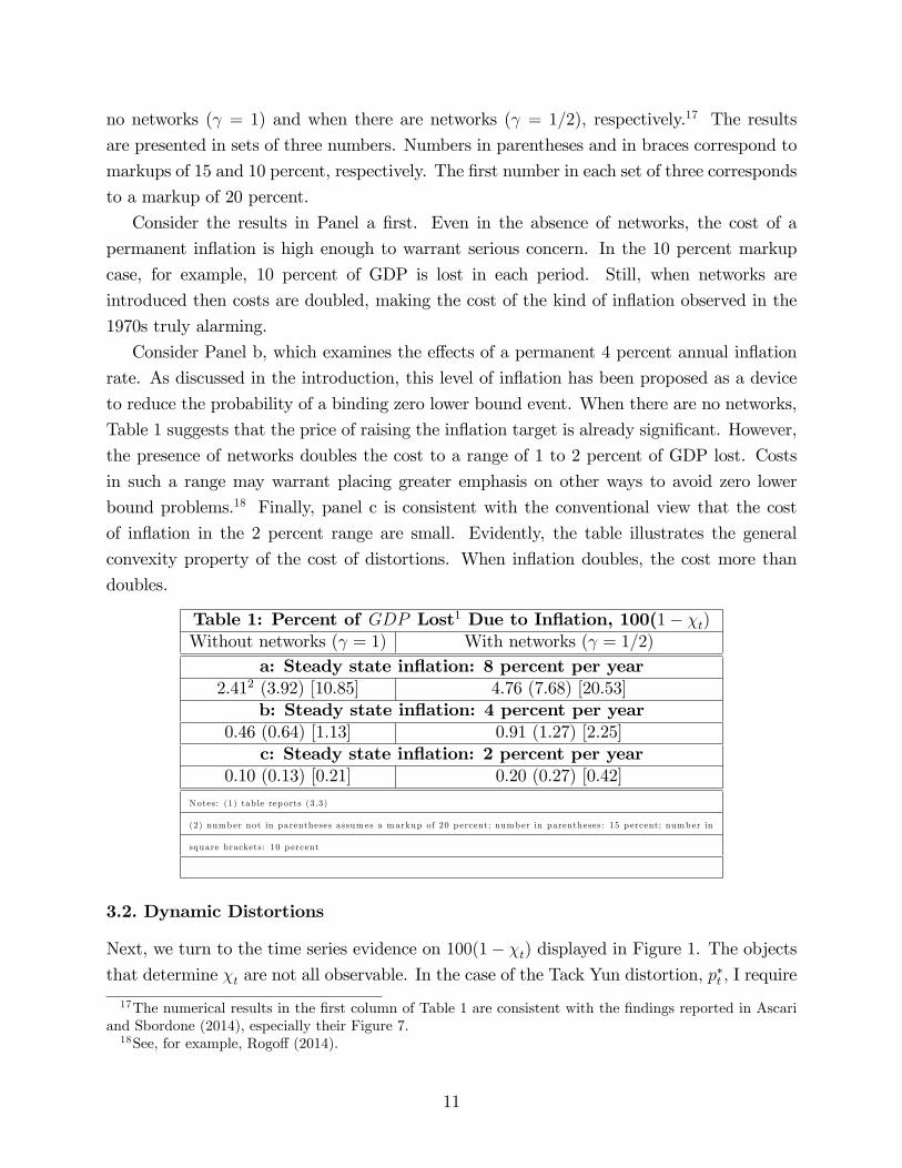
no networks (γ = 1) and when there are networks (γ = 1/2), respectively.17 The results

are presented in sets of three numbers. Numbers in parentheses and in braces correspond to

markups of 15 and 10 percent, respectively. The first number in each set of three corresponds

to a markup of 20 percent.

Consider the results in Panel a first. Even in the absence of networks, the cost of a

permanent inflation is high enough to warrant serious concern. In the 10 percent markup

case, for example, 10 percent of GDP is lost in each period. Still, when networks are

introduced then costs are doubled, making the cost of the kind of inflation observed in the

1970s truly alarming.

Consider Panel b, which examines the effects of a permanent 4 percent annual inflation

rate. As discussed in the introduction, this level of inflation has been proposed as a device

to reduce the probability of a binding zero lower bound event. When there are no networks,

Table 1 suggests that the price of raising the inflation target is already significant. However,

the presence of networks doubles the cost to a range of 1 to 2 percent of GDP lost. Costs

in such a range may warrant placing greater emphasis on other ways to avoid zero lower

bound problems.18 Finally, panel c is consistent with the conventional view that the cost

of inflation in the 2 percent range are small. Evidently, the table illustrates the general

convexity property of the cost of distortions. When inflation doubles, the cost more than

doubles.

Table 1: Percent of GDP Lost1 Due to Inflation, 100(1− χt)Without networks (γ = 1) With networks (γ = 1/2)

a: Steady state inflation: 8 percent per year2.412 (3.92) [10.85] 4.76 (7.68) [20.53]

b: Steady state inflation: 4 percent per year0.46 (0.64) [1.13] 0.91 (1.27) [2.25]

c: Steady state inflation: 2 percent per year0.10 (0.13) [0.21] 0.20 (0.27) [0.42]

Notes: (1) tab le rep orts (3 .3)

(2) number not in parentheses assum es a markup of 20 p ercent; number in parentheses: 15 p ercent; number in

square brackets: 10 p ercent

3.2. Dynamic Distortions

Next, we turn to the time series evidence on 100(1− χt) displayed in Figure 1. The objectsthat determine χt are not all observable. In the case of the Tack Yun distortion, p

∗t , I require

17The numerical results in the first column of Table 1 are consistent with the findings reported in Ascariand Sbordone (2014), especially their Figure 7.18See, for example, Rogoff (2014).

11

an initial condition (see (2.4)). However, I found that the initial condition has a negligible

dynamic effect on p∗t . Figure 1 reports the time series on p∗t when the initial value of p

∗t (in

1947Q3) is set to unity. The results after 1960 are essentially unchanged if I instead set the

initial condition to the much lower value of 0.80.

To compute χt I also need time series data on µt/p∗t in order to construct ωt (see (2.8)).

For the reasons explained in section 2, I adopt the approximation, ωt = 1.19

Figure 1 has two panels. Figures 1a and 1b display results for the case where the markup

is 20 percent and 15 percent, respectively. Each panel displays three time series: quarterly

observations on quarterly gross inflation in the consumer price index; quarterly observations

on 100(1− p∗t ) and quarterly observations on 100(1− χt) = 100(1− (p∗t )1/γ).

Consider panel a first. There are several notable results. First, the percent of GDP

lost when it is assumed there are networks is roughly twice as large when the network

structure of production is ignored (I set γ = 1/2). Second, the losses due to inflation can be

quantitatively large. In normal, low inflation, times, the average cost is well below 1 percent

but when inflation rises a bit, the costs rise sharply.

In panel b the costs are higher. On average, 2.65 percent of GDP is lost. Also, more

than 4 percent of GDP is lost in 18 percent of the 273 quarters considered. And, in those

quarters the average loss of GDP was 10 percent. Finally, the losses during the high inflation

of the 1970s are quantitatively large. Indeed, they reach a maximum value of over 20 percent

during the high inflation period (see Figure 1b). The average loss in the high inflation period

was 9.73 percent of GDP per period, according to the results in Figure 1b. This exceeds the

7.68 percent loss reported in Table 1a because of the convexity of the loss as a function of

inflation. These numbers certainly vindicate the conventional view that the cost of the high

inflation in the 1970s was high.

Clearly, the NK model has no trouble rationalizing the view that high inflation imposes

a big cost on society. If anything, one is suspicious that the cost suggested by the model is

implausibly high.

4. Networks and the Slope of the Phillips Curve

The standard Phillips curve reported in the literature only holds when there are no price

distortions in the steady state. When there are price distortions - as most of the discussion

here assumes - then the Phillips curve is more complicated than and includes additional

19See the first approximate equality in (2.9). The approximation depends crucially on ν = ν∗. In practice,this greatly exaggerates the role of the tax system in undoing monopoly distortions. (Indeed, actual thetax systems provide their own distortions.) However, some preliminary calculations suggest that allowingmonopoly power to also reduce χt by setting ν = 0 has only a small impact on the contribution of inflationto χt.

12

variables. Still, to preserve comparability I display the usual Phillips curve for the special

case when there is no steady state inflation. For the same reason, I also drop working capital,

so that ψ = 0. The appendix shows that the Phillips curve for this model is:

πt =(1− θ) (1− βθ)

θγ (1 + ϕ)xt + βEtπt+1, (4.1)

where πt ≡ πt − 1 denotes the net inflation rate. Also, xt represents the output gap, the log

of the ratio of GDP (i.e., consumption) to potential GDP. As explained in the Appendix,

potential GDP can be interpreted either as the level of output that would occur if prices

were flexible, or the level of output in the Ramsey equilibrium. The key thing to note in

(4.1) is that the slope of the Phillips curve in terms of the output gap is cut in half by the

presence of networks.20 The underlying intuition, based on strategic complementarities, is

explained in the introduction.

5. Networks and the Taylor Principle

There is a consensus that inflation targeting is a monetary policy with excellent operating

characteristics, at least in ‘normal’times when the zero lower bound on the interest rate is

not binding. Inflation targeting can be operationalized by applying a rule like (2.10) with a

coeffi cient on inflation that is substantially greater than unity, i.e., that satisfies the ‘Taylor

principle’. The idea is that the Taylor principle serves two important objectives. One is the

achievement of low average inflation. By raising the interest rate when inflation is above

target, the central bank reigns in the demand for goods and services. Working through

the demand channel, this policy generates a slowdown in economic activity, which brings

inflation back down to target by reducing marginal costs.

The second objective of the Taylor principle is to anchor inflation expectations. Unan-

chored inflation expectations can be a source of instability in inflation as well as in aggregate

output and employment. To see this, suppose that for some reason there is a jump in inflation

expectations. The resulting lower real rate of interest stimulates spending and output. By

producing a rise in marginal cost, the increase in output contributes to a rise in inflation. In

this way, the initial jump in inflation expectations is self-fulfilling and so inflation is without

an anchor.

The Taylor principle helps to short-circuit this loop from higher inflation expectations to

higher actual inflation. This is also accomplished by working through the demand channel.

When the monetary authority raises the interest rate vigorously in response to inflation, the

demand channel produces a fall in spending which reduces output and hence inflation. As

people become aware of the lower actual inflation, the inflation expectations that initiated

20Here, and throughout, I assume that the empirically plausible value of γ is 1/2.

13

the loop would evaporate before it could have much of an effect on the macroeconomy. Under

rational expectations, the initial rise in inflation expectations would not occur in the first

place.

The stabilizing effects of the Taylor principle depend on the demand channel being the

primary avenue through which monetary policy operates. When firms have to borrow to pay

for their variable inputs, then the interest rate is a part of marginal cost and monetary policy

also operates through a working capital channel. If the working capital channel is suffi ciently

important then, instead of curbing inflation, a jump in the nominal rate of interest could

actually ignite inflation.

Whether the working capital or demand channel dominate has been studied extensively

in the type of model described in the previous section.21 The general finding is that when

γ = 1 the demand channel dominates the working capital channel and the Taylor principle

achieves the two objectives described above. This is so, even when the working capital

channel is strongest, with ψ = 1. When gross output and value added coincide, there is

not enough borrowing for the working capital channel to overwhelm the demand channel.

However, when we take into account the network nature of production (i.e., γ = 2), then the

amount of borrowing for working capital purposes is potentially much greater. As a result,

when ψ = 1 and there is no interest rate smoothing in the Taylor rule, i.e., ρ = 0, the non-

stochastic steady state equilibrium is indeterminate. Even though monetary policy satisfies

the Taylor principle, there are many equilibria. These equilibria can be characterized in

terms of the loop from higher expected inflation to higher actual inflation discussed above.

When there is no working capital channel, then the Taylor principle short-circuits this loop

by raising the interest rate and preventing the rise in expected inflation from occurring.

But, when the working capital channel is suffi ciently strong, then the rise in the interest rate

simply reinforces the loop from higher expected inflation to higher actual inflation. In this

way the Taylor principle could become the ‘Taylor curse’referred to in the introduction.

It is interesting that the Taylor principle works as hoped for when there is substantial

interest rate smoothing in monetary policy, i.e., ρ is large. Presumably, the intuition for this

is that demand responds most strongly to long term interest rates rather than to short term

interest rates. As a result, the strength of the demand channel is increasing in ρ while the

working capital channel, which is only a function of the short term interest rate, remains

unaffected.

The example highlights how the integration of network effects could be important for the

design of monetary policy. This is a topic that deserves further study. It is important to

know, for example, how pervasive working capital is in the data.22 It is also important to

21See Christiano, Trabandt and Walentin (2011).22For one revelant study, see Barth and Ramey (2002).

14

understand better how the working capital channel works in network environments that are

closer to the more realistic one advocated in the Acemoglu et al paper, in which firms buy

materials directly from other firms.

6. Conclusion

Acemoglu et al suggest that the introduction of networks into macroeconomic models could

have first-order consequences for the kinds of questions that interest macroeconomists. I

have described three examples in which this is the case. The examples convince me that

following the lead of Acemoglu et al and others by integrating networks into macroeconomics

represents an important priority.

A. Appendix: Model Used in the Analysis

This comment makes use of a standard NK model, extended to include network effects

following the suggestion of Basu (1995). At the level of detail, the model corresponds to the

one analyzed in Christiano, Trabandt and Walentin (2011) (CTW). I include a description of

the model in this appendix for three reasons. First, CTW do not describe all the connections

between gross output and value-added that I use in my discussion. Second, I explain the

properties of the first-best allocations discussed in the text. Third, the text loosely describes

some subtleties associated with the Phillips curve in the present context, and the appendix

explains these carefully. Fourth, conclusions from stochastic simulations of the model are

summarized in section 3 and the discussions in sections 4 and 5 are also based on analyses

that make use of all parts of the model.

A.1. Households

There are many identical, competitive households who maximize utility,

maxE0

∞∑t=0

βt(u (Ct)−

N1+ϕt

1 + ϕ

), u (Ct) ≡ logCt,

subject to the following budget constraint:

s.t. PtCt +Bt+1 ≤ WtNt +Rt−1Bt + Profits net of taxest.

Here, Ct denotes consumption; Wt denotes the nominal wage rate; Nt denotes employment;

Pt denotes the nominal price of consumption; Bt+1 denotes a nominal one period bond

purchased in period t which pays off a gross, nominal non-state contingent return, Rt, in

15

period t + 1. Also, the household earns lump sum profits and pays lump sum taxes to the

government. Optimization by households implies:

1

Ct= βEt

1

Ct+1

Rt

πt+1

(A.1)

CtNϕt =

Wt

Pt. (A.2)

A.2. Goods Production

The structure of production has the Dixit-Stiglitz structure that is standard in the NK

literature, extended to consider network effects.

A.2.1. Homogeneous Goods

A representative, homogenous good firm produces output, Yt, using the following technology:

Yt =

[∫ 1

0

Yε−1ε

i,t dj

] εε−1

, ε > 1. (A.3)

The firm takes the price of homogeneous goods, Pt, and the prices of intermediate goods,

Pi,t, as given and maximizes profits,

PtYt −∫ 1

0

Pi,tYi,tdj,

subject to (A.3). Optimization leads to the following first order condition:

Yi,t = Yt

(PtPi,t

)ε, (A.4)

for all i ∈ (0, 1) . Combining the first order condition with the production function, we obtain

the following equilibrium condition:

Pt =

(∫ 1

0

P(1−ε)i,t di

) 11−ε

. (A.5)

A.2.2. Intermediate Goods

The intermediate good, i ∈ (0, 1) , is produced by a monopolist using the following technol-

ogy:

Yi,t = AtNγi,tI

1−γi,t , 0 < γ ≤ 1.

Here, Ni,t and Ii,t denotes the quantity of labor and materials, respectively, used by the ith

producer. The producer obtains Ii,t by purchasing the homogenous good, Yt, and converting

it one-for-one into materials. Both Ni,t and Ii,t are acquired in competitive markets.

16

Firms experience Calvo-style frictions in setting their price. That is, the ith firm sets its

period t price, Pi,t, as follows:

Pi,t =

{Pt with probability 1− θPi,t−1 with probability θ

, 0 ≤ θ < 1. (A.6)

Here, Pt denotes the price selected in the probability 1− θ event that it can choose its price.Firms that cannot optimize their price must simply set it to whatever value it took on in

the previous period.

Given its current price (however arrived at), the firm must satisfy the Yit that is implied

by (A.4). Linear homogeneity of its technology and our assumption that the ith firm acquires

materials and labor in competitive markets implies that marginal cost is independent of Yi,t.

By studying its cost minimization problem we find that st, the ith firm’s marginal cost (scaled

by Pt) is

st =

(Pt/Pt1− γ

)1−γ (Wt/Ptγ

)γ1

At. (A.7)

Here, Pt and Wt denote the net price, after taxes and interest rate costs, of materials and

labor, respectively. In particular,

Wt = (1− ν) (1− ψ + ψRt)Wt

Pt = (1− ν) (1− ψ + ψRt)Pt,

where ψ represents the fraction of input costs that must be financed in advance so that, for

example, one unit of labor used during period t costs ψWtRt units of currency at the end of

the period.23 Also, ν is the subsidy discussed in the text.

Another implication of the ith firm’s cost minimization problem is that cost of materials,

PtIi,t, as a fraction of total cost, is equal to 1− γ. This implies,

Ii,t = µtYi,t, (A.8)

where µt is the share of materials in gross output, and:

µt =(1− γ) st

(1− ν) (1− ψ + ψRt). (A.9)

I now turn to the problem of one of the 1 − θ randomly selected firms that has an

opportunity to select its price, Pt, in period t. Such a firm is concerned about the value of

its cash flow (i.e., revenues net of costs) in period t and in later periods:

Et

∞∑j=0

(βθ)j υt+j

[PtYi,t+j − Pt+jst+jYi,t+j

]+ Φt. (A.10)

23We assume that banks create credits which they provide in the amount, (ψWtNt + ψPtIt) , to firms atthe beginning of the period. At the end of the period they receive Rt (ψWtNt + ψPtIt) back from firms andthe profits, (Rt − 1) (ψWtNt + ψPtIt) , are transferred to households in lump sum form.

17

The objects in square brackets are the cash flows in current and future states in which the firm

does not have an opportunity to reset its price. The expectation operator in (A.10) integrates

over aggregate uncertainty, while the firm-level idiosyncratic uncertainty is manifest in the

presence of θ in the discounting. In (A.10), cash flows in each period are weighed by the

associated date and state-contingent value that the household assigns to cash. The firm

takes these weights as given and

υt+j =u′ (Ct+j)

Pt+j. (A.11)

The second term in (A.10), Φt, represents the value of cash flow in future states in which

the firm is able to reset its price. Given the structure of our environment, Φt is not affected

by the choice of Pt. The problem of a firm that is able to choose its price is to select a value

of Pt that maximizes (A.10) subject to (A.4), taking Pt, Wt, Pt and Wt as given.

To solve the firm problem I first substitute out for Yi,t and υt using (A.4) and (A.11),

respectively. I then differentiate (A.10) taking into account that Φt is independent of Pt.

The solution to this problem is obtained by a standard set of manipulations. In particular,

let

pt ≡PtPt, πt ≡

PtPt−1

, Xt,j =

{ 1πt+j πt+j−1···πt+1 , j ≥ 1

1, j = 0.,

Xt,j = Xt+1,j−11

πt+1

, j > 0

Then, the (scaled by Pt) solution to the firm problem is:

pt =Et∑∞

j=0 (βθ)j (Xt,j)−ε Yt+j

Ct+j

εε−1

st+j

Et∑∞

j=0 (βθ)j (Xt,j)1−ε Yt+j

Ct+j

=Kt

Ft, (A.12)

where

Kt =ε

ε− 1

YtCtst + βθEt

(1

πt+1

)−εKt+1 (A.13)

Ft =YtCt

+ βθEt

(1

πt+1

)1−ε

Ft+1. (A.14)

A.3. Economy-wide Variables and Equilibrium

By the usual result associated with Calvo-sticky prices, we have the following cross-price

restriction:

Pt =

(∫ 1

0

P(1−ε)i,t di

) 11−ε

=[(1− θ) P (1−ε)

t + θP(1−ε)t−1

] 11−ε

. (A.15)

18

Dividing by Pt and rearranging,

pt =

[1− θπ(ε−1)

t

1− θ

] 11−ε

. (A.16)

Combining this expression with (A.12), we obtain a useful equilibrium condition:

Kt

Ft=

[1− θπ(ε−1)

t

1− θ

] 11−ε

. (A.17)

It is convenient to express real marginal cost, (A.7), in terms that do not involve prices:

st = (1− ν) (1− ψ + ψRt)

(1

1− γ

)1−γ (1

γCtN

ϕt

)γ1

At, (A.18)

where (A.2) has been used to substitute out for Wt/Pt.

I now derive the value-added production function. To this end, we first compute the

equilibrium relationship between aggregate inputs, It and Nt, and gross output, Yt. I do this

by adapting the argument in Yun (1996). I then adapt a version of the argument in Jones

(2013) to obtain the mapping from aggregate employment to GDP.

Let Y ∗t denote the unweighted sum of Yi,t and then substitute out for Yi,t in terms of

prices using (A.4):

Y ∗t ≡∫ 1

0

Yi,tdi = Yt

∫ 1

0

(Pi,tPt

)−εdi = Yt

(PtP ∗t

)ε,

where

P ∗t ≡[∫ 1

0

P−εi,t di

]−1ε

=[(1− θ) P−εt + θ

(P ∗t−1

)−ε]−1ε, (A.19)

using the analog of the result in (A.15). In this way, we obtain the following expression for

Yt :

Yt = p∗tY∗t , p

∗t ≡

(P ∗tPt

)ε,

p∗t =

{≤ 1 not Pi,t = Pj,t, all i, j= 1 Pi,t = Pj,t, all i, j

,

where p∗t is the Tack Yun distortion discussed in the text.

By a standard calculation, I obtain the law of motion for p∗t by dividing (A.19) by P∗t ,

using (A.16) and rearranging,

p∗t =

(1− θ)(

1− θπ(ε−1)t

1− θ

) εε−1

+θπεtp∗t−1

−1

. (A.20)

19

Then,

Yt = p∗tY∗t = p∗t

∫ 1

0

Yi,tdi = p∗tAt

∫ 1

0

Nγi,tI

1−γi,t di

= p∗tAt

(Nt

It

)γIt,

where I have used the fact that all firms have the same materials to labor ratio. In this way,

we obtain

Yt = p∗tAtNγt I

1−γt . (A.21)

I substitute out for It in (A.21) by noting from (A.8) that

It ≡∫ 1

0

Ii,tdi = µt

∫ 1

0

Yi,tdi = µtY∗t =

µtp∗tYt. (A.22)

Use this to solve out for It in (A.21):

Yt =

(p∗tAt

(µtp∗t

)1−γ) 1

γ

Nt. (A.23)

GDP for this economy is simply

Ct = Yt − It. (A.24)

I conclude,

GDPt = Yt − It =

(1− µt

p∗t

)Yt = FN,t ×Nt, (A.25)

after some rearranging. Here, TFP denotes total factor productivity and is given by:

FN,t =

(p∗tAt

(1− µt

p∗t

)γ (µtp∗t

)1−γ) 1

γ

, (A.26)

or,

FN,t = χt(Atγ

γ (1− γ)1−γ) 1γ ,where

χt ≡

p∗t(

1− µtp∗t

γ

)γ ( µtp∗t

1− γ

)1−γ 1

γ

. (A.27)

There are 12 variables to be determined for the model:

Kt, Ft, πt, p∗t , st, Ct, Yt, Nt, It, µt, Rt, χt.

There are 11 equilibrium conditions implied by private sector decisions : (A.13), (A.14),

(A.17), (A.20), (A.1), (A.21), (A.24), (A.23), (A.18), (A.9), (A.27). In the special case of

20

flexible prices (θ = 0) and no working capital (ψ = 0) then the classical dichotomy obtains.

That is, equilibrium consumption and employment can be solved and, given the subsidy in

(2.2), we obtain:

Nt = 1, Ct =[At (γ)γ (1− γ)1−γ] 1γ .

In the case that is of interest in this discussion, we need an additional equation to solve the

model variables. To this end, I adopt the specification of monetary policy, (2.10). It can be

verified that the steady state of the model is determinate when the smoothing parameter is

0.8 but indeterminate when the smoothing parameter is zero. The economic reasons for this

are discussed in section 5.

To compute the dynamic properties of the model I solve the model using second order

perturbation (with pruning), using Dynare.24 For this, I require the model steady state

in which the shocks, at, are held at their steady state values of zero. The steady state is

discussed in the next section.

The parameter values I assign to the model are as follows:

π = 1.02514 , ψ = 1, γ =

1

2, β = 1.03−0.25,

θ = 0.75, ε = 6, ϕ = 1, ν = ν∗.

The time series representation I use for at is that it is roughly a first order autoregression in

its first difference. In particular,

at = (ρ1 + ρ2) at−1 − ρ1ρ2at−2 + εt, Eε2t = 0.012,

where ρ1 = 0.99 and ρ2 = 0.3.

A.4. Model Steady State

This section displays the steady state of the model. I derive the steady state expressions,

(2.2) and (3.2), as well as the result that L in (2.1) is equal to unity when ν = ν∗. In

addition, the steady state is required in the next subsection to derive the linearized Phillips

curve which is discussed in the text.

Removing the time subscripts from time series variables in the model equilibrium condi-

tions, (A.1), (A.17), (A.13), (A.14), (A.20), we find:

R =π

β, Kf ≡

K

F=

[1− θ

1− θπ(ε−1)

] 1ε−1

,

s = Kfε− 1

ε

1− βθπε1− βθπε−1

, p∗ =1− θπε1− θ

(1− θ

1− θπ(ε−1)

) εε−1

(A.28)

24The code is available on my website.

21

The steady state share of materials in costs, scaled by p∗, is given by

µ

p∗=

(1− γ) s/p∗

(1− ν) (1− ψ + ψR), (A.29)

according to (A.9). Let ν∗ be defined by,

µ

p∗= (1− γ)

1− ν∗1− ν . (A.30)

Equating (A.29) and (A.30), and using (A.28), we obtain (2.2). This establishes (3.2).

In steady state the marginal product of labor is

FN =

[p∗(

1− (1− γ)1− ν∗1− ν

)γ ((1− γ)

1− ν∗1− ν

)1−γ] 1γ

=

(p∗

(1− (1− γ) 1−ν∗

1−νγ

)γ (1− ν∗1− ν

)1−γ) 1

γ (γγ (1− γ)1−γ) 1γ , (A.31)

using (A.26) and (A.30).

According to (A.29) and (A.30),

s = (1− ψ + ψR) (1− ν∗) p∗.

Using this expression to substitute out for s in the steady state version of (A.18),

1− ν∗1− ν p

∗ (1− γ)1−γ (γ)γ = (CNϕ)γ ,

using the fact, At = 1, in steady state. Combining the last expression with (A.31), we obtain

1− ν∗1− ν

F γN(

1−(1−γ) 1−ν∗

1−νγ

)γ (1−ν∗1−ν)1−γ

= (CNϕ)γ .

After rearranging, the latter expression reduces toγ

γ + ν∗−ν1−ν∗

= L. (A.32)

From this we can see the result cited in the text, that L = 1 when ν = ν∗.

We can solve (A.32) for N by using C = FNN :

N =

[γ

γ + ν∗−ν1−ν∗

] 11+ϕ

.

Finally,

C = FNN, Y =C

γ,

I = (1− γ)Y, F =1/γ

1− βθπε−1, K = Kf × F,

so that all steady state variables are now available.

22

A.5. Output Gap

The output gap is a key variable in the Phillips curve and I discuss that variable here. The

output gap is the log deviation of equilibrium output from a benchmark level of output. Three

possible benchmarks include: (i) output in the Ramsey equilibrium, (ii) the equilibrium when

prices are flexible and (iii) the first best equilibrium, when output is chosen by a benevolent

planner. In the latter case this corresponds to maximizing25

u (Ct)−N1+ϕt

1 + ϕ

subject to the maximal level of consumption that can be produced by allocating resources

effi ciently across sectors:

Ct =(Atγ

γ (1− γ)1−γ) 1γ Nt.

Optimization implies:

C∗t =(Atγ

γ (1− γ)1−γ) 1γ , N∗t = 1. (A.33)

It is easily verified that when there is no working capital channel, ψ = 0, then (i), (ii) and

(iii) coincide (that the equilibrium allocations under flexible prices are given by (A.33) was

discuss in section A.3). With ψ > 0 the three benchmarks differ. In this case expressions

(i) and (ii) are relatively complicated, while (iii) stands out for its analytic simplicity. This

is why I work with (iii) as my benchmark. This leads me to the following definition of the

output gap, Xt :

Xt =CtC∗t.

The log deviation from the steady state is:

xt ≡ Xt = Ct − C∗t= Ct −

1

γAt, (A.34)

where xt is also log (Xt/X) for Xt suffi ciently close to its steady state value, X.

A.6. Phillips Curve

Linearizing (A.13), (A.14) and (A.17), about steady state,

Kt = (1− βθπε)[Yt + st − Ct

]+ βθπεEt

(επt+1 + Kt+1

)(A.35)

Ft =(1− βθπε−1

) (Yt − Ct

)+ βθπε−1Et

((ε− 1) πt+1 + Ft+1

)(A.36)

Kt = Ft +θπ(ε−1)

1− θπ(ε−1)πt. (A.37)

25I assume the planner has the capacity to avoid the frictions associated with working capital, when ψ > 0.

23

Here, xt = (xt − x) /x and x denotes the steady state value of xt. Substitute out for Kt in

(A.35) using (A.37) and then substituting out for Ft using (A.36), we obtain,(1− βθπε−1

) (Yt − Ct

)+ βθπε−1Et

((ε− 1) πt+1 + Ft+1

)+

θπ(ε−1)

1− θπ(ε−1)πt = (1− βθπε)

[Yt + st − Ct

]+ βθπεEt

(επt+1 + Ft+1 +

θπ(ε−1)

1− θπ(ε−1)πt+1

).

Collecting terms,

πt =

(1− θπ(ε−1)

)(1− βθπε)

θπ(ε−1)st + βEtπt+1 (A.38)

+ (1− π)(1− θπ(ε−1)

)β

[Yt − Ct + Et

(Ft+1 +

(ε+

θπ(ε−1)

1− θπ(ε−1)

) πt+1

)].

This expression reduces to the usual Phillips curve in the special case, π = 1.

We require st. Combining (A.2), (A.25) and (A.7),

st = (1− ν) (1− ψ + ψRt)

(1

1− γ

)1−γ (1

γC1+ϕt

)γTFP−ϕγt

At.

Totally differentiating,

st =ψR

(1− ψ + ψR)Rt + (1 + ϕ) γCt − ϕγTFP t − At.

We obtain TFP t by totally differentiating (A.26):

TFP t =1

γAt,

where terms in p∗t and µt disappear because we set π = 1. Then,

st =ψR

(1− ψ + ψR)Rt + γ (1 + ϕ)

[Ct −

1

γAt

].

Using (A.34), this establishes:

st =ψR

(1− ψ + ψR)Rt + γ (1 + ϕ)xt.

Substituting this expression for marginal cost into (A.38) with π = 1, we obtain the rep-

resentation of the Phillips curve displayed in the text. The object, xt, is a conventional

measure of the output gap when ψ = 0. When ψ > 0 it must be interpreted as the percent

deviation between actual and first best output (see section A.5).

24

References

[1] Alvarez, Fernando, Martin Gonzalez-Rozada, Andy Neumeyer and Martin Beraja, 2011,

‘From Hyperinflation to Stable Prices: Argentina’s Evidence on Menu Cost Models,’

unpublished manuscript.

[2] Ascari, Guido, 2004, ‘Staggered prices and trend inflation: some nuisances,’Review of

Economic Dynamics 7, pp, 642—667.

[3] Ascari, Guido and Argia M. Sbordone, 2014, ‘The Macroeconomics of Trend Inflation,’

Staff Report No. 628, Federal Reserve Bank of New York.

[4] Ascari, Guido, Louis Phaneuf and Eric Sims, 2015, ‘On the Welfare and Cyclical Impli-

cations of Moderate Trend Inflation,’National Bureau of Economic Research Working

Paper 21392.

[5] Ball, Larry, 2013, ‘The case for 4% inflation,’ May 24, VOX,

http://www.voxeu.org/article/case-4-inflation.

[6] Barth III, M.J., Ramey, V.A., 2002, ‘The cost channel of monetary transmission,’ in

Bernanke, B., Rogoff, K.S., editors, NBER Macroeconomics Annual 2001, MIT Press,

Cambridge, MA, pp. 199—256.

[7] Basu, Susanto, 1995, ‘Intermediate goods and business cycles: Implications for produc-

tivity and welfare,’American Economic Review, 85 (3), 512—531.

[8] Blanchard, Olivier, 1987, “Aggregate and Individual Price Adjustment,”Brookings Pa-

pers on Economic Activity, vol. 1.

[9] Calvo, Guillermo A., 1983, ‘Staggered Prices in a Utility-maximizing Framework,’Jour-

nal of Monetary Economics 12 (3), 383—398.

[10] Christiano, Lawrence J., Martin Eichenbaum and Charles Evans, 2005, ‘Nominal Rigidi-

ties and the Dynamic Effects of a Shock to Monetary Policy,’Journal of Political Econ-

omy, 113 (1), 1—45.

[11] Christiano, Lawrence J., Cosmin Ilut, Roberto Motto and Massimo Rostagno, 2010,

‘Monetary Policy and Stock Market Booms,’in Federal Reserve Bank of Kansas City

Economic Policy Symposium in Jackson Hole, Wyoming, Macroeconomic Challenges:

The Decade Ahead.

25

[12] Christiano, Lawrence J., Mathias Trabandt, and Karl Walentin, 2011, ‘DSGEModels for

Monetary Policy Analysis,’In Benjamin M. Friedman, and Michael Woodford, editors:

Handbook of Monetary Economics, Vol. 3A, The Netherlands: North-Holland, 2011, pp.

285-367.

[13] Eichenbaum, Martin, Nir Jaimovich, and Sergio Rebelo, 2011, ‘Reference Prices and

Nominal Rigidities,’American Economic Review 101 (1): 234—62.

[14] Golosov, Mikhail and Robert E. Lucas, Jr., 2007, ‘Menu Costs and Phillips Curves,’

Journal of Political Economy, vol. 115, no. 2.

[15] Gordon, Robert J., 1981, ‘Output Fluctuations and Gradual Price Adjustment,’Journal

of Economic Literature, vol. 19 (June), p. 525.

[16] Huang, Kevin X.D. and Zheng Liu, 2001, ‘Production chains and general equilibrium

aggregate dynamics,’Journal of Monetary Economics, 48, 437-462.

[17] Huang, Kevin X.D. and Zheng Liu, 2005, ‘Inflation targeting: What inflation rate to

target?,’Journal of Monetary Economics, 52, 1435—1462.

[18] Jones, Chad, 2013, ‘Misallocation, Economic Growth, and Input-Output Economics,’

in D. Acemoglu, M. Arellano, and E. Dekel, Advances in Economics and Econometrics,

Tenth World Congress, Volume II, Cambridge University Press.

[19] Krugman, Paul R., 1997, The Age of Diminished Expectations: US Economic Policy in

the 1990s, MIT Press.

[20] Nakamura, Emi and Jon Steinsson, 2010, ‘Monetary Non-Neutrality in a Multisector

Menu Cost Model,’The Quarterly Journal of Economics, August 2010.

[21] Rogoff, Kenneth, 2014, ‘Costs and benefits to phasing out paper currency,’ NBER

Macroeconomics Annual 2014, Volume 29.

[22] Rotemberg, Julio, and Michael Woodford, 1993, ‘Dynamic General Equilibrium Models

with Imperfectly Competitive Product Markets,’National Bureau of Economic Research

Working Paper number 4502.

[23] Yun, Tack, 1996, ‘Nominal Price Rigidity, Money Supply Endogeneity, and Business

Cycles,’Journal of Monetary Economics, 37 (2), 345—370.

26