discriminative correlation filters for visual tracking
TRANSCRIPT
Discriminative Correlation Filters for Visual TrackingMartin Danelljan

Overview – Part I
Part I: Basics of Discriminative Correlation Filters
1. The Visual Tracking problem
2. DCF – the simple case
3. Multi-channel, multi-sample DCF
4. Special cases and approximative inference
5. Tracking pipeline and practical considerations
6. Kernels
7. Scale estimation
8. Periodic assumption: problem and solutions
Overview – Part II
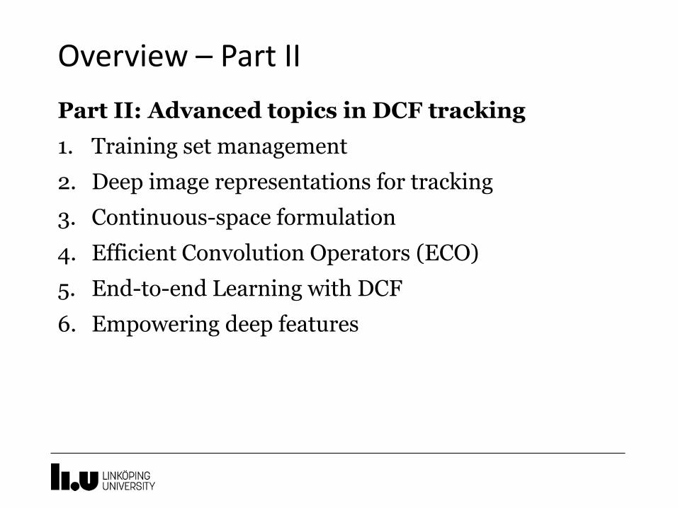
Part II: Advanced topics in DCF tracking
1. Training set management
2. Deep image representations for tracking
3. Continuous-space formulation
4. Efficient Convolution Operators (ECO)
5. End-to-end Learning with DCF
6. Empowering deep features

Visual Tracking

Visual Tracking

Visual Tracking
• Only initial target location in known
• Challenges
– Environmental: occlusions, blur, clutter, illumination
– Motion/transformations: rotations, fast motion, scale change
– Appearance changes: deformations

Applications
Robotics, AR/VR, autonomous driving, video analysis …

Discriminative Correlation Filters (DCF)- The Basics

Discriminative Correlation Filters
What is it?
• Discriminatively learn a correlation filter
• Utilize the Fourier transform for efficiency
Why use it?
• Translation invariance ⇒ Correlation
• State-of-the-art since 2014
• Accuracy (even sub-pixel)
• Generic and customizable

DCF Popularity and Performance
• Hundreds of papers since 2014
• Winner of Visual Object Tracking (VOT) Challenge 2014, 2016, 2017 and 2018
• In VOT 2018: all top-5 trackers are based on DCF

DCF – the Simple Case
DFT

DCF – the Simple Case

DCF – the Simple Case
Target prediction:


Standard DCF Formulation
1. Multiple training samples
2. Multidimensional sophisticated features

Standard DCF Formulation

Standard DCF Formulation
weights

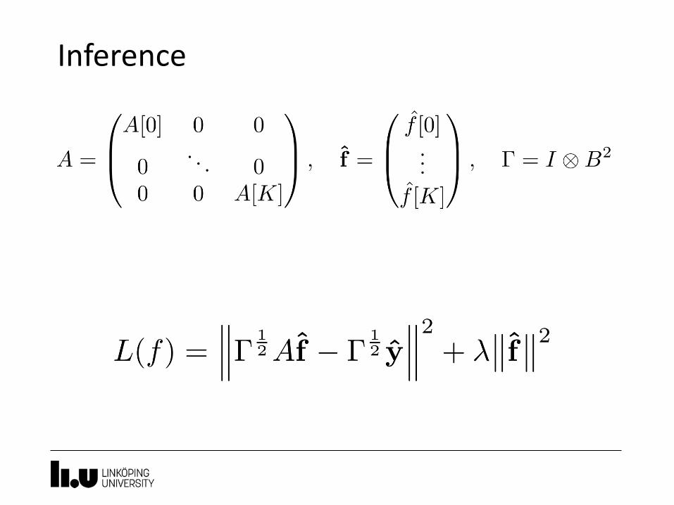
Inference
• DFT and Parseval’s theorem:

Inference
Inference

Inference

Inference
Blocks of 𝑚 × 𝐷
Blocks of D × 𝐷
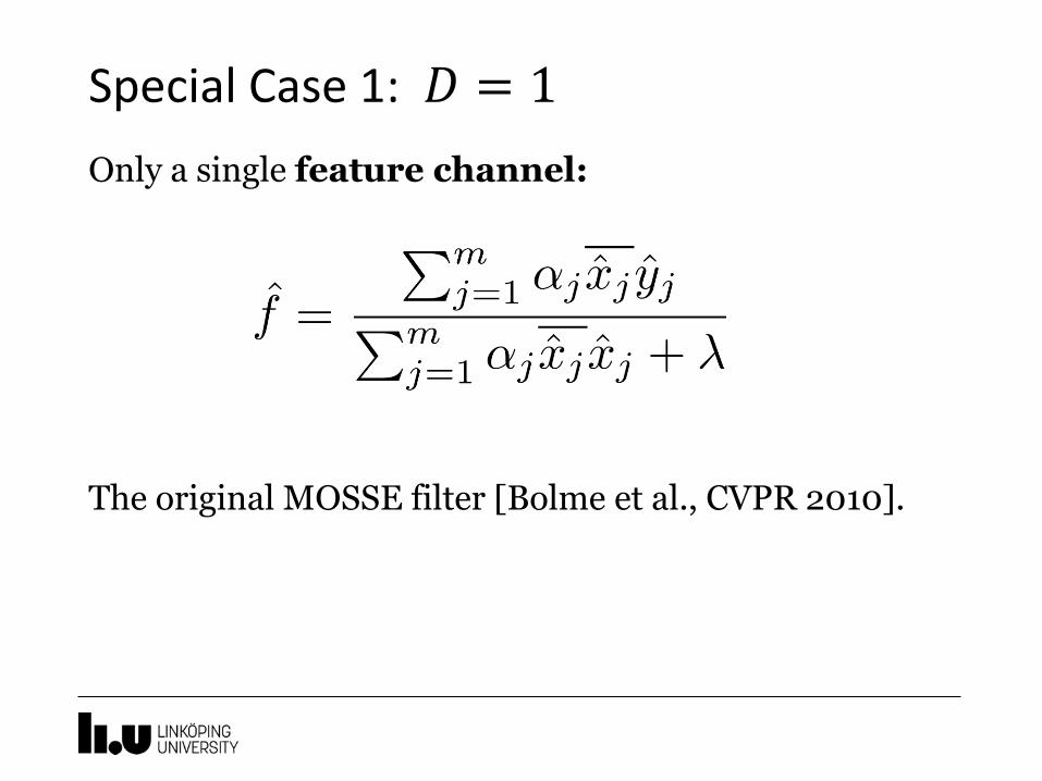
Special Case 1: 𝐷 = 1
Only a single feature channel:
The original MOSSE filter [Bolme et al., CVPR 2010].

Dual form
Blocks of 𝑚 ×𝑚

Special Case 2: m = 1
Only a single training sample:
[Danelljan et al., BMVC 2014, PAMI 2017]

Approximate inference
1. Independent samples:
– Optimal for 𝑚 = 1
2. Independent channels:
– Optimal for D = 1
3. Combination:
– Optimal for 𝑚 = 1
– Optimal for D = 1

General tracking pipeline
1. Initialize model in first frame
2. Track in the new frame
3. Update model and goto 2.

Tracking pipeline: example
1. Initialize
2. Track
3. UpdateTarget location
Learning rate

Practical considerations
1. Multiply samples with cosine window
– Reduces boundary effects

Practical considerations
2. For : use Gaussian function
– Centered at target location
– Peak width parameter
– Motivation: minimizes the uncertainty principle

Kernelized Correlation Filters

Kernelized Correlation Filters (KCF)
• Henriques et al. [ECCV 2012, PAMI 2014]
• Idea: apply the kernel trick to the DCF
Kernel:
Shift invariant:
Example:
Shift operator:

Kernelized Correlation Filters (KCF)
• Kernelized correlation:
• Train model:
• Target scores:
• Approximative update rules [Henriques et al., 2012; Danelljan et al., 2014].

Kernelized Correlation Filters (KCF)
Should you use kernels?
More complicated learning
Harder to generalize
More costly
Similar or poorer performance
Essence of deep learning:
- Learn you feature mapping instead

Scale Estimation
Martin Danelljan, Gustav Häger, Fahad Shahbaz Khan, and Michael Felsberg. “Discriminative Scale Space Tracking”. In: IEEE Transactions on Pattern Analysis and Machine Intelligence 39.8 (2017), pp. 1561–1575.

Scale Estimation

Approach 1: Multi-scale detection
1. Extract test samples at multiple scales
2. Compute scores at each scale
3. Find max position and scale
…
…
Approach 2: Scale filter
• Idea: train a separate 1-dimensional scale DCF
• Directly discriminates between scales
• Discriminative Scale Space Tracker (DSST)[Danelljan et al., BMVC 2014, PAMI 2017]

Discriminative Scale Space Tracker
Scale training sample x Desired output y
Targ
et s
ize
Confidence score

Discriminative Scale Space Tracker

Discriminative Scale Space Tracker

Evaluation Measures
Predicted box
Ground-truth box

Scale Estimation Results
OTB-2013 dataset[Wu et al., CVPR 2013]

Scale estimation: Comparison
Approach 2 (scale filter):
• Faster
• Generic (used in many different trackers)
• Often more accurate for simple DCF trackers
Approach 1 (multi-scale detection):
• Slower
• Often more accurate for advanced DCF trackers
presented next

The Periodic Assumption: Problem and Solutions

Periodic Assumption in DCF
What we want… What actually happens…

Larger Samples?

Why?
Learned filter

Effects of Periodic Assumption
Forces a small sample size in training/detection
Effects:
• Limits training data
• Corrupts data
• Limits search region

Tackling the Periodic Assumption
We need means of controlling the filter extent!
• Enables larger samples.
Approaches:
1. Constrained optimization
2. Spatial regularization

Constrained Optimization
• Idea: Constrain filter coefficients to be zero outside the target bounding box.
• Rewrite constraint:
background pixels
Inverse Fourier transform

Constrained Optimization
• Fourier domain formulation:
target pixels

Constrained Optimization
• Generates dense normal equations
• Use iterative solvers:
– ADMM [H.K. Galoogahi, CVPR 2015]
– Proximal gradient [J.A. Fernandez, PAMI 2015]
• Requires iterating between spatial and Fourier

Spatially Regularized DCF (SRDCF)[M. Danelljan, ICCV 2015]

Spatially Regularized DCF (SRDCF)[M. Danelljan, ICCV 2015]

Spatially Regularized DCF (SRDCF)
DFT

Spatially Regularized DCF (SRDCF)
DFT

Spatially Regularized DCF (SRDCF)
Convolution matrix
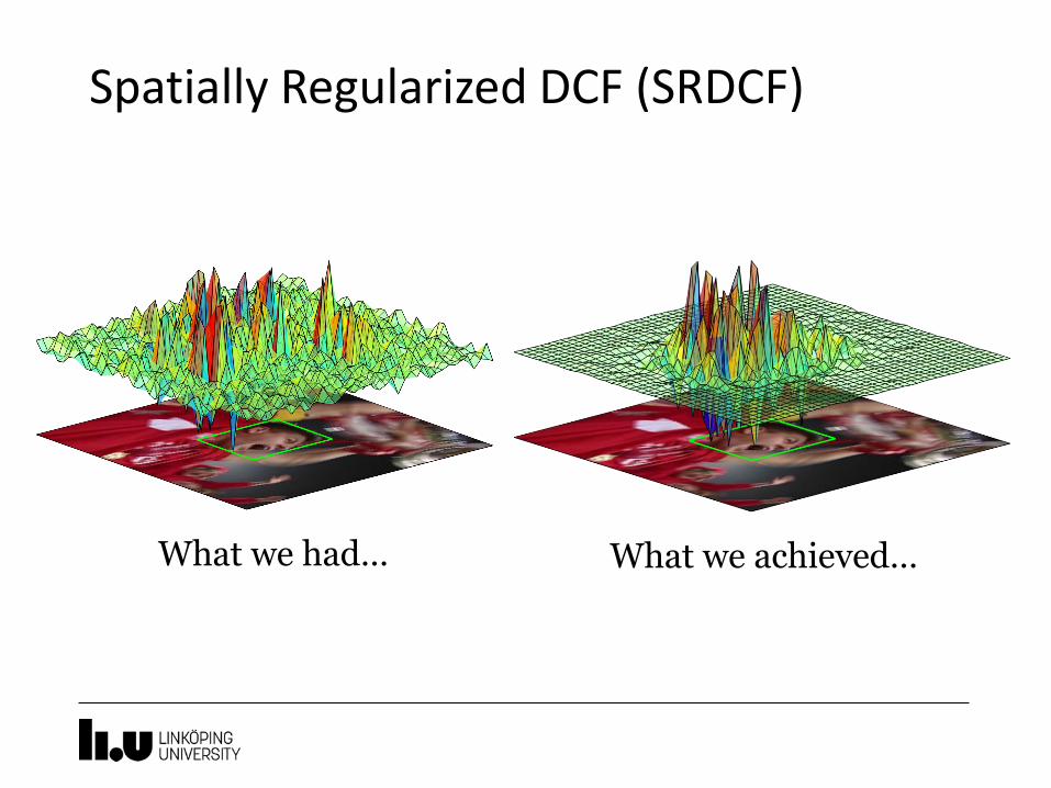
Spatially Regularized DCF (SRDCF)
What we had… What we achieved…

Spatially Regularized DCF

Spatially Regularized DCF

Spatially Regularized DCF
OTB-2015 dataset

Adaptive Training Set Management
Martin Danelljan, Gustav Häger, Fahad Shahbaz Khan, and Michael Felsberg. “Adaptive Decontamination of the Training Set: A Unified Formulation for Discriminative Visual Tracking”. In: IEEE Conference on Computer Vision and Pattern Recognition, CVPR 2016.

Model Drift

Adaptive Training Set Management

Discriminative Tracking Methods

Our Approach - Motivation
• Continuous weights
– More control of importance
– Helps in ambiguous cases (e.g. partial occlusions)
• Re-determination of importance in each frame
– Exploit later samples
– Use all available information
• Prior information
– E.g. how old the sample is
– Or number of samples in a frame

Our Approach

Adaptive Sample Weights

Deep Image Representations For Tracking

Hand-crafted FeaturesColor Features[M. Danelljan, CVPR 2014]
Color Names[Weijer and Schmid, TIP 2009]
Shape features
Histogram of Oriented Gradients (HOG)[Dalal and Triggs, 2005]

Deep Convolutional Features

Evaluation of Convolutional Feature Layers
• On OTB-2013 dataset
[M. Danelljan, ICCVW 2015]
Learning Continuous Convolution Operators
Martin Danelljan, Andreas Robinson, Fahad Shahbaz Khan, and Michael Felsberg. “Beyond Correlation Filters: Learning Continuous Convolution Operators for Visual Tracking”. In: European Conference on Computer Vision (ECCV) 2016.

Discriminative Correlation Filters (DCF)
Single-resolution feature map
Limitations:Coarse output
scores

Our Approach: Overview
Continuous filters Continuous
outputMulti-
resolution features

DCF Limitations:1. Single-resolution feature map
• Why a problem?
– Combine convolutional layers of a CNN
• Shallow layers: low invariance – high resolution
• Deep layers: high invariance – low resolution
• How to solve?
– Explicit resampling?
• Artefacts, information loss, redundant data
– Independent DCFs with late fusion?
• Sub-optimal, correlations between layers

DCF Limitations:2. Coarse output scores
• Why a problem?
– Accurate localization
• Sub-grid (e.g. HOG grid) or sub-pixel accuracy
• More accurate annotations=> less drift
• How to solve?
– Interpolation?
• Which interpolation strategy?
– Interweaving?
• Costly
DCF Limitations:3. Coarse labels
• Why a problem?
– Accurate learning
• Sub-grid or sub-pixel supervision
• How to solve?
– Interweaving?
• Costly
– Explicit interpolation of features?
• Artefacts

Interpolation Operator

Convolution Operator

Training Loss

Training Loss – Fourier Domain

Optimization: Conjugate Gradient
• Solve
• Use Conjugate Gradient:
– Only need to evaluate
– => No sparse matrix handling!
– Warm start estimate and search direction
– Preconditioner important
• Details: “On the Optimization of Advanced DCF-Trackers”, J. Johnander, G. Bhat, M. Danelljan, F. Khan, M. Felsberg. VOT Challenge ECCV Workshop, 2018.

How to set and ?
• Use periodic summation of functions :
• Gaussian function for
• Cubic spline kernel for
• Fourier coefficients with Poisson’s summation formula:

Results
• Layer fusion on OTB-2015 dataset
75
76
77
78
79
80
81
82
83
Conv1 Conv1 + Conv5 RGB + Conv1 +Conv5
Mea
n O
verl
ap P
reci
sio
n +3.8% +0.6%

Sub-pixel Localization with CCOT

Sub-pixel Localization with CCOT

Feature Point Tracking Framework
• Grayscale pixel features,
• Uniform regularization,

CCOT Feature Point Tracking

Experiments: Feature Point Tracking
• The Sintel dataset

Efficient Convolution Operators (ECO)
Martin Danelljan, Goutam Bhat, Fahad Shahbaz Khan, and Michael Felsberg. “ECO: Efficient Convolution Operators for Tracking”. In: IEEE Conference on Computer Vision and Pattern Recognition CVPR 2017.

Issues With C-COT
1. Slow
– ~10 FPS with hand-crafted features
– ~1 FPS with deep features
2. Overfitting
– ~0.5M parameters updated online
– Memory focusing on recent samples

Factorized Convolution
• Learn filter 𝑓 and matrix 𝑃 jointly
• Gauss Newton iterations with Conjugate Gradient
• 80% reduction in parameters
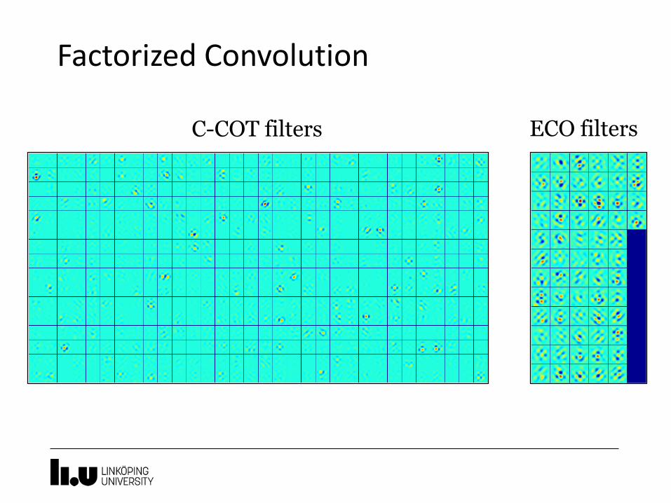
Factorized Convolution
C-COT filters ECO filters

Generative Sample Space Model
• Online Gaussian Mixture Model of training samples
• ⟹ 90% reduction in training samples
ECO:GMM clusters
Previous:Linear memory

Speedup
• 10x speedup compared to C-COT
• Same or better performance
• 60 FPS on CPU with handcrafted features
• 15 FPS on GPU with deep features
Notes:
• Matlab/Mex
• “Slow” network

End-to-end Learning with DCF

End-to-end Learning
• Could we learn the underlying features?
• Use the DCF solution for a single training sample as a layer in a deep network:
• Train in Siamese fashion:
– On image pairs
Network parameters
test sample
desired output

End-to-end Learning: CFNet
[J. Valmadre et al., CVPR 2017]
• Logistic loss

End-to-end Learning: CFCF
[E. Gondogdu and A. Alatan, TIP 2018]
• 𝐿2-loss. Finetune VGG-m.
• Integrate learned features in C-COT

Unveiling the Power of Deep Tracking
Goutam Bhat, Joakim Johnander, Martin Danelljan, Fahad Shahbaz Khan, and Michael Felsberg. “Unveiling the Power of Deep Tracking”. In: European Conference on Computer Vision (ECCV) 2018.

ECOTracking Performance, NFS

104
Motivation
• Challenges: Deformations, In-plane/Out-of-plane rotations
• Can we utilize the invariance of deep features?

105
Motivation
• How about using deeper networks?
Tracking Performance, NFS

106
Motivation
• Features unsuitable for tracking?
– Let's train features for tracking
Tracking Performance, NFS

107
Causes 1: Training data
• Limited training data in the first frame
• Training data only models translations

108
Data augmentation
• Can simulate commonly encountered challenges in object tracking, e.g. rotations, motion blur, occlusions

109
Data augmentationImpact of data augmentation, OTB-2015
Deep: ResNet-50 (Conv4)
Shallow: HOG+Color Names

110
Cause 2: Accuracy-Robustness Tradeoff
Image Shallow Model Deep Model

111
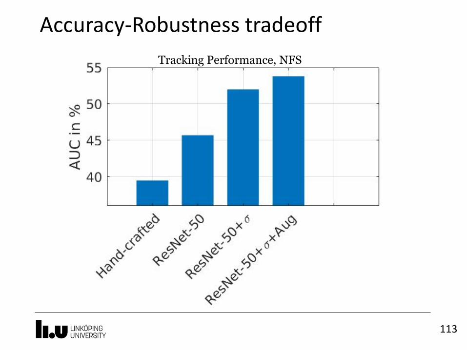
Cause 2: Accuracy-Robustness Tradeoff
Let’s revisit training in ECO
• Training data: Shifted versions of the target
• Width of label function determines how the samples are labelled
• Sharp label function ⇒ Enforce Accuracy
• Wide label function ⇒ Prefer Robustness

112
Cause 2: Accuracy-Robustness TradeoffImpact of label width, OTB-2015
Deep: ResNet-50 (Conv4)
Shallow: HOG+Color Names
113
Accuracy-Robustness tradeoff
Tracking Performance, NFS

114
Accuracy-Robustness tradeoff
Image Shallow Model Deep Model

115
New framework
Extract Features
Shallow
Deep
Train Separate Filters Apply filter
Fusion?

116
Adaptive Model Fusion
We want the score function to have a single, sharp peak
Image Deep Score Shallow Score

117
Adaptive Model Fusion
• Prediction Quality Measure

118
Results
Need For Speed dataset (100 videos)

119
Results
Generalization to networks

State-of-the-Art and Conclusions

Current state-of-the-art
• VOT2018 sequestered dataset
Directly based on ECO
[“The Visual Object Tracking VOT2018 Challenge Results”, M. Kristan et al., 2018]

Conclusions and Future Work
• DCF is a versatile framework for tracking
• Highly adaptable for specific applications
• Efficient online learning
• Future work:
– Richer output: towards segmentation
– Long-term tracking robustness
– Better end-to-end integration and learning

Gustav Häger Fahad Khan Michael FelsbergGoutam Bhat Joakim Johnander
Acknowledgements
• EMC2, funded by Vetenskapsrådet
• Wallenberg AI, Autonomous Systems and Software Program (WASP) funded by the Knut and Alice Wallenberg Foundation

www.liu.se
Martin Danelljan