discrimination of acceptable and contaminated heparin by
TRANSCRIPT

DISCRIMINATION OF ACCEPTABLE AND CONTAMINATED HEPARIN BY
CHEMOMETRIC ANALYSIS OF PROTON NUCLEAR MAGNETIC
RESONANCE SPECTRAL DATA
By
Qingda Zang
A Dissertation Submitted to
the University of Medicine and Dentistry of New Jersey – School of
Health Related Professions in partial fulfillment of the Requirements for
the Degree of Doctor of Philosophy
Department of Health Informatics
April, 2011
ii

iii
ABSTRACT
DISCRIMINATION OF ACCEPTABLE AND CONTAMINATED HEPARIN BY
CHEMOMETRIC ANALYSIS OF PROTON NUCLEAR MAGNETIC
RESONANCE SPECTRAL DATA
Qingda Zang
Heparin is a highly effective anticoagulant that can contain varying
amounts of undesirable galactosamine impurities (mostly dermatan sulfate or
DS), the level of which indicates the purity of the drug substance. Currently,
the United States Pharmacopeia (USP) monograph for heparin purity dictates
that the weight percent of galactosamine in total hexosamine (%Gal) may not
exceed 1%. In 2007 and 2008, heparin contaminated with oversulfated
chondroitin sulfate (OSCS) was associated with adverse clinical effects, i.e., a
rapid and acute onset of a potentially fatal anaphylactoid-type reaction. In
order to develop efficient and reliable screening methods for detecting and
identifying contaminants in existing and future lots of heparin to ensure the
integrity of the global supply, chemometric techniques for heparin proton
nuclear magnetic resonance (1H NMR) spectral data were applied to establish
adequate multivariate statistical models for discrimination between pure
heparin samples and those deemed unacceptable based on their levels of DS
and/or OSCS.

iv
The whole research work consisted of two parts: (1) the development of
quantitative regression models to predict the %Gal in various heparin
samples from NMR spectral data. Multivariate analyses including multiple
linear regression (MLR), Ridge regression (RR), partial least squares
regression (PLSR), and support vector regression (SVR) were employed in
this investigation. To obtain stable and robust models with high predictive
ability, variables were selected by genetic algorithms (GA) and stepwise
methods; (2) differentiation of heparin samples from impurities and
contaminants by the different pattern recognition and classification
approaches, such as principal components analysis (PCA), partial least
squares discriminant analysis (PLS-DA), linear discriminant analysis (LDA), k-
nearest-neighbor (kNN), classification and regression tree (CART), artificial
neural networks (ANN) and support vector machine (SVM), as well as the
class modeling techniques soft-independent modeling of class analogy
(SIMCA) and unequal dispersed classes (UNEQ).
Overall, the results from this study demonstrate that NMR spectroscopy
coupled with multivariate chemometric techniques shows promise as a
valuable tool for evaluating the quality of heparin sodium active
pharmaceutical ingredients (APIs). These developed models may be useful in
monitoring purity of other complex pharmaceutical products from high
information content data.

v
ACKNOWLEDGEMENTS
I would like to acknowledge my advisor Dr. Dinesh P. Mital for his inspiring
supervision and supportive attitudes. The completion of this dissertation could
not have been possible without his invaluable guidance and unending
patience.
I wish to express my gratitude to my co-advisor, Dr. William J. Welsh who
has given me the opportunity to be where I am today. I would like to thank
him for trusting me and letting me go my own way.
I want to express my sincere thanks to the faculty members at the
Department of Health Informatics, especially to Dr. Syed S. Haque, Dr.
Shankar Srinivasan, and Dr. Masayuki Shibata, for their expertise, training,
advice and assistance throughout my graduate study.
I am very grateful to Dr. Richard D. Wood at Snowdon, Inc. for his
stimulating discussion, timely encouragement and constructive suggestions.
I would also like to thank the staff at the US Food and Drug Administration
(FDA). They provided the analysis data and more importantly, the financial
support, which made the research work possible. The collaboration with them
has greatly broadened my perspectives and I have learned a great deal from
them. Special thanks to Dr. Lucinda F. Buhse, Dr. David A. Keire, Dr.
Christine M. V. Moore, Dr. Moheb Nasr, Dr. Ali Al-Hakim, and Dr. Michael L.
Trehy.
vi
I would like to extend my gratitude to Dr. Dmitriy Chekmarev at the
Department of Pharmacology for spending his time in reviewing this
dissertation and valuable comments and feed-back.
Finally, I wish to thank my colleagues at Dr. Welsh‟s group, Dr. Ni Ai, Dr.
Vladyslav Kholodovych, Dr. Eric Kaipeen Yang and Dr. Oyenike Olabisi for
their consistent enthusiasm and reliable willingness to help, and friendly and
pleasant environment.

vii
TABLE OF CONTENTS
ABSTRACT ..................................................................................................... iii
ACKNOWLEDGEMENTS ............................................................................... v
LIST OF TABLES ............................................................................................ix
LIST OF FIGURES ..........................................................................................xi
Chapter I. INTRODUCTION ............................................................................ 1
1.1 Statement of the Problem ...................................................................... 1
1.2 Background of the Problem ................................................................... 4
1.3 Objectives of the Research .................................................................... 7
1.4 Research Hypotheses ........................................................................... 9
1.5 Results and Significance of the Research ........................................... 11
Chapter II. LITERATURE REVIEW ............................................................... 16
2.1 The Structure, Preparation and Medical Use of Heparin ..................... 17
2.1.1 Structures of Glycosaminoglycans (GAGs) ................................... 17
2.1.2 Preparation of Heparin .................................................................. 21
2.1.3 Medical Use of Heparin ................................................................. 22
2.2 Heparin Crisis ...................................................................................... 24
2.2.1 Adverse Events ............................................................................. 25
2.2.2 Contaminant Identification ............................................................. 26
2.2.3 USP Monograph for Heparin Quality ............................................. 32
2.3 Chemometrics and its Application in Heparin Field ............................. 33
2.3.1 Variable Selection ......................................................................... 34
2.3.2 Multivariate Regression Analysis .................................................. 39
2.3.3 Chemometric Pattern Recognition ................................................ 46
2.3.4 Application of Chemometrics in Heparin Field .............................. 67
Chapter III. DATA AND METHODS .............................................................. 72
3.1 Heparin Samples ................................................................................. 72
3.1.1 Pure, Impure and Contaminated Heparin APIs for Classification .. 72
3.1.2 Heparin API Samples for %Gal Determination .............................. 73
3.1.3 Blends of Heparin Spiked with other GAGs .................................. 74
3.2 Proton NMR Spectra............................................................................ 75
3.3 Data Processing .................................................................................. 77
viii
3.4 Computational Programs ..................................................................... 79
3.5 Performance Validation ....................................................................... 80
Chapter IV. RESULTS AND DISCUSSION ................................................... 82
4.1 Multivariate Regression Analysis for Predicting %Gal ......................... 82
4.1.1 Variable Selection ......................................................................... 82
4.1.2 Multiple Linear Regression Analysis ............................................. 90
4.1.3 Ridge Regression Analysis ........................................................... 97
4.1.4 Partial Least Squares Regression Analysis ................................ 101
4.1.5 Support Vector Regression Analysis ........................................... 105
4.2 Classification of Pure and Contaminated Heparin Samples .............. 108
4.2.1 Principal Components Analysis ................................................... 110
4.2.2 Partial Least Squares Discriminant Analysis ............................... 115
4.2.3 Linear Discriminant Analysis ....................................................... 119
4.2.4 k-Nearest-Neighbor ..................................................................... 123
4.2.5 Classification and Regression Tree ............................................. 128
4.2.6 Artificial Neural Networks ............................................................ 133
4.2.7 Support Vector Machine .............................................................. 137
4.2.8 Analysis of Misclassifications ...................................................... 141
4.2.9 Classification Analysis of Heparin Spiked with other GAGs ........ 145
4.3 Class Modeling for Discriminating Heparin Samples ......................... 149
4.3.1 SIMCA Analysis .......................................................................... 149
4.3.2 UNEQ Analysis ........................................................................... 165
Chapter V. SUMMARY AND CONCLUSIONS ............................................ 173
5.1 Multivariate Regression for Predicting %Gal ..................................... 173
5.2 Classification for Pure and Contaminated Heparin Samples ............. 175
5.3 Class Modeling Using SIMCA and UNEQ ......................................... 180
Chapter VI. FUTURE DIRECTION FOR RESEARCH ................................ 184
References .................................................................................................. 188
Appendix A: Abbreviations .......................................................................... 204
Appendix B: Index ....................................................................................... 207
ix
LIST OF TABLES
Table 1. Summary Statistics of %Gal Measured from HPLC ........................... 74
Table 2. Variable IDs and their Corresponding Chemical Shifts ...................... 79
Table 3. The Stepwise Variable Selection Procedure for Dataset A ............... 85
Table 4. The Stepwise Variable Selection Procedure for Dataset B ............... 86
Table 5. Parameters for the Genetic Algorithms ................................................ 87
Table 6. The Variables (ppm) Selected by Genetic Algorithms ....................... 89
Table 7. Model Parameters of Multiple Linear Regression (MLR) ................... 92
Table 8. Model Parameters of Ridge Regression (RR) ................................... 100
Table 9. Model Parameters of Partial Least Squares Regression (PLSR) .. 104
Table 10. Model Parameters for Support Vector Regression with RBF Kernel................................................................................................................................... 107
Table 11. Number and Type of Misclassifications (Errors) by PLS-DA Classification ........................................................................................................... 118
Table 12. Wilks‟ Lambda ( v ) & F-to-enter (F) of Variables (V) for Various
Models ...................................................................................................................... 120
Table 13. Performance of LDA Classification Models under Different Variables .................................................................................................................. 121
Table 14. Performance of kNN Classification Models for Original Data ....... 124
Table 15. Performance of PCA-kNN Classification Models under Different PCs ........................................................................................................................... 125
Table 16. Model Parameters and Classification Rates for CART .................. 130
Table 17. Model Parameters and Classification Rates for ANN .................... 137

x
Table 18. Model Parameters and Classification Rates for SVM .................... 141
Table 19. Classification Matrices for the Heparin vs DS Model in the 1.95-5.70 ppm Region .................................................................................................... 143
Table 20. Classification Matrices for the Heparin vs [DS + OSCS] Model in the 1.95-5.70 ppm Region .................................................................................... 144
Table 21. Classification Matrices for the Heparin vs DS vs OSCS Model in the 1.95-5.70 ppm Region ........................................................................................... 144
Table 22. Compositions of the Series of Blends of Heparin Spiked with other GAGs and Test Results for Classification from SVM, CART and ANN in the 1.95-5.70 ppm Region ........................................................................................... 148
Table 23. Sensitivity and Specificity from SIMCA Modeling for Heparin, DS, and OSCS ............................................................................................................... 151
Table 24. Classification Matrices and Success Rates from SIMCA Class Modeling for Heparin, DS and OSCS ................................................................. 157
Table 25. Discriminant Powers (DP) of Variables (V) for Various Models ... 161
Table 26. The Compositions of the Series of Blends of Heparin Spiked with other GAGs and Test Results from Class Modeling ......................................... 164
Table 27. Wilks Lambda (λ) and F-to-enter (F) Values of Variables (V) ....... 167
Table 28. Sensitivity and Specificity from UNEQ Class Modeling for Heparin, DS and OSCS ......................................................................................................... 169
Table 29. Classification Matrices from UNEQ Class Modeling for Heparin, DS and OSCS ............................................................................................................... 172

xi
LIST OF FIGURES
Figure 1. Three-dimensional structures of heparin. ........................................... 18
Figure 2. Structural formulae of heparin, dermatan sulfate, chondroitin sulfate A and C, and oversulfated chondroitin sulfate ..................................................... 19
Figure 3. Monthly event date distributions of heparin allergic-type reports received from January 1, 2007 to September 30, 2008 ..................................... 26
Figure 4. NMR analysis of standard heparin, heparin containing natural dermatan sulfate and contaminated heparin ....................................................... 29
Figure 5. The molecular structures of heparin and OSCS ................................ 30
Figure 6. Schematic diagram representing the process of assessing sample class from raw NMR spectra .................................................................................. 49
Figure 7. Structure of a classification or regression tree .................................. 56
Figure 8. A fully connected multilayer feedforward network ............................. 58
Figure 9. Non-linear separation case in the low dimension input space and linear separation case in the high dimension feature space ............................. 61
Figure 10. Scores plot of the PCA analysis of the spectral data set ............... 69
Figure 11. Separation of the samples containing OSCS from those not containing OSCS in a score-plot of a PCA model .............................................. 70
Figure 12. Comparison of Raman spectra of heparin and the principal contaminants and Raman PLS model test for OSCS ........................................ 71
Figure 13. An overlay of the 500MHz 1H NMR spectra of a heparin sodium API spiked with 10.0% of CSA, OS-CSA, CSB and OS-CSB. .......................... 76
Figure 14. The relationship between the Bayes information criterion (BIC) and the number of variables selected by the stepwise procedure ................... 84
Figure 15. Histograms of frequency for the selected variables by GAs ......... 88
Figure 16. Predicted (from NMR data) versus measured (from HPLC) %Gal for Dataset A (%Gal: 0-10) ..................................................................................... 93

xii
Figure 17. Predicted (from NMR data) versus measured (from HPLC) %Gal for Dataset B (%Gal: 0-2) ........................................................................................ 96
Figure 18. Ridge regression for the heparin 1H NMR data at 40 variables selected from GA ...................................................................................................... 99
Figure 19. The relationship between the component number of PLSR and the standard error of prediction (SEP) for Dataset A .............................................. 102
Figure 20. Scores plots for the model Heparin vs DS ..................................... 112
Figure 21. Scores plots for the model Heparin vs OSCS ............................... 113
Figure 22. Scores plots for the model Heparin vs DS vs OSCS .................... 114
Figure 23. Misclassification rate as a function of the number of PLS components for the PLS-DA model ..................................................................... 116
Figure 24. kNN classification for heparin-contaminant data over the range k =1 to k = 25 ............................................................................................................. 127
Figure 25. Classification trees and their corresponding complexity parameter CP for model Heparin vs DS vs OSCS ............................................................... 129
Figure 26. The variations of misclassification errors from ANN with the hidden units and weight decay for the model Heparin vs DS vs OSCS for the data set in the 1.95-5.70 ppm range ................................................................... 136
Figure 27. Contour plots obtained from 9×9 grid search of the optimal values of γ and C for the SVM model .............................................................................. 140
Figure 28. Dendrogram on the blends of heparin spiked with other GAGs 147
Figure 29. Coomans plots for SIMCA class modeling ..................................... 153
Figure 30. Coomans plots for UNEQ class modeling ...................................... 171
Figure 31. Comparison of the classification results of the six approaches .. 179
Figure 32. Overlaid plots of the SAX-HPLC chromatograms ......................... 185
Figure 33. Near infrared spectra of 108 heparin samples that contain DS impurities and OSCS contaminants .................................................................... 186

1
Chapter I
INTRODUCTION
1.1 Statement of the Problem
Heparin, a highly sulfated glycosaminoglycan, is widely used as an
anticoagulant. This drug substance is obtained from biological sources and
always contains varying amounts of undesirable impurities. Among these,
chondroitin sulfate A (CSA) and chondroitin sulfate B (i.e., dermatan sulfate or
DS) have been identified. These chondroitin derivatives differ from heparin in
that they contain galactosamine, the level of which is used as an indicator for
the quality of the drug. Currently, the United States Pharmacopeia (USP)
monograph for heparin purity dictates that the weight percent of
galactosamine (%Gal) may not exceed 1%. Hence the accurate
measurement of the %Gal in heparin is an important parameter to assure the
safety and efficacy of the drug. The experimental determination of %Gal by
acid digestion and high-performance liquid chromatography (HPLC) with a
pulsed amperometric detector requires expert operators, expensive
equipment and careful sample preparation. By contrast, although the nuclear
magnetic resonance (NMR) approach requires more expensive equipment
than the HPLC method, the sample preparation is minimal and the data are
already required for other aspects of USP testing. Therefore, the development
of theoretical methods for the prediction of %Gal values from NMR spectral
data is of particular interest.

2
In late 2007 and early 2008, heparin sodium contaminated with
oversulfated chondroitin sulfate A (OSCS) was associated with a rapid and
acute onset of an anaphylactic reaction. In addition, naturally occurring
dermatan sulfate (DS) with concentrations up to a few percent was found to
be present in heparin samples as an impurity due to incomplete purification. It
is desirable to develop simple and effective screening analytical methods for
detecting and identifying contaminants and impurities in existing and future
lots of heparin. Because unique signals associated with OSCS or DS in
contaminated or impure heparin were observed in the NMR spectra, the
present study was undertaken to determine whether chemometric statistical
analysis of these NMR spectral data would be useful for discrimination
between USP-grade samples of heparin sodium active pharmaceutical
ingredients (APIs) and those deemed unacceptable based on their levels of
OSCS and/or DS. For this purpose, pattern recognition techniques for 1H
NMR spectral data were applied to establish adequate mathematical models
for revealing similarities and differences between heparin and contaminants.
In order to differentiate heparin samples with varying amount of DS
impurities and OSCS contaminants, proton NMR spectral data for heparin
sodium API samples from different manufacturers were analyzed by
multivariate statistical methods for quantitative determination and qualitative
classification. The whole research work was divided into two parts, i.e.,
multivariate regression analysis for the prediction of %Gal and pattern

3
recognition analysis for the differentiation of pure, impure and contaminated
heparin samples.
1. The quantitative determination of %Gal. This combination of
spectroscopy and chemometric methods was proposed for the prediction of
%Gal. Multivariate analyses including multiple linear regression (MLR), Ridge
regression (RR), partial least squares regression (PLSR), and support vector
regression (SVR) were employed in the present investigation. To obtain
stable and robust models with high predictive ability, variables were selected
by genetic algorithms (GAs) and stepwise methods.
2. Discrimination of pure, impure and contaminated heparin samples.
Heparin sample classifications were performed by applying multivariate
statistical approaches such as principal component analysis (PCA), partial
least squares discriminant analysis (PLS-DA), linear discriminant analysis
(LDA), k-nearest neighbors (kNN), classification and regression tree (CART),
artificial neural network (ANN), support vector machine (SVM), as well as
class-modeling techniques, such as soft-independent modeling of class
analogy (SIMCA) and unequal dispersed classes (UNEQ) for analysis of
proton NMR spectral data in order to distinguish between pure, impure and
contaminated heparin. The NMR signals were employed as fingerprints, and
classification models were built and validated for the determination of the
contaminant and/or impurity in the lots of heparin.

4
1.2 Background of the Problem
Heparin is a naturally occurring polydisperse mixture of linear, highly
sulfated carbohydrates composed of repeating disaccharide units, which
generally comprise a 6-O-sulfated, N-sulfated glucosamine alternating with a
2-O-sulfated iduronic acid [1-3]. As a member of the glycosaminoglycan
(GAG) family, heparin has the highest negative charge density among known
biological molecules. During heparin biosynthesis, the polysaccharide chains
are incompletely modified and variably elongated, leading to heterogeneity in
chemical structure, diversity in sulfation patterns, and polydispersity in
molecular mass [4]. As one of the oldest drugs still in widespread clinical use,
heparin is highly effective in kidney dialysis and cardiac surgery. Heparin is
the most widely used anticoagulant for preventing or treating thromboembolic
disorders, and for inhibiting coagulation during hemodialysis and
extracorporeal blood circulation [5-8].
Pharmaceutical heparin is usually derived by extracting animal tissues,
such as bovine, ovine, and porcine intestinal mucosa or bovine lung after
proteolytic digestion, and then precipitating the preparations as quaternary
ammonium complexes or barium salts, and eventually as sodium or calcium
salts [9-12]. Crude heparin contains proteins, nucleic acid, and other related
GAGs, such as heparan sulfate (HS), dermatan sulfate (DS), chondroitin
sulfate (CS), and hyaluronic acid (HA) [13]. Subsequent purification by
proprietary processes converts raw heparin into active pharmaceutical

5
ingredients (APIs) and the differences in these processes leads to variation in
the amount of native impurities in the final product [14, 15]. Dermatan sulfate
(DS) is the most common chondroitin sulfate impurity in heparin. DS is
composed of alternating iduronic acid-galactosamine disaccharide units and,
due to their similarity with the iduronic-glucosamine disaccharide units of
heparin, heparin APIs always contain varying levels of DS owing to the strong
affinity as well as incomplete purification [16]. The stage 2 USP monograph
for heparin sodium limits %Gal to not more than 1%. To ensure the
appropriate biological activity, chemical parameters, including purity,
molecular mass distribution, degree of sulfation, as well as the presence of
specific oligosaccharide sequences, must be strictly controlled. It is difficult to
accurately determine the precise chemical structure and to measure the
performance of purification protocol due to the heterogeneity of heparin
preparations [17-20].
Starting in November 2007, hundreds of cases of adverse reactions to
heparin, such as hypotension, severe allergic symptoms, and even death in
patients undergoing hemodialysis and receiving bolus injections of heparin
sodium, were reported to the US Food and Drug Administration (FDA) [21-
23]. Prompted by these adverse events, biological and analytical methods
were developed to identify contaminants and impurities in heparin [14, 15, 24-
28]. Oversulfated chondroitin sulfate (OSCS) was identified as a contaminant
associated with these adverse clinical effects. In standard drug potency
6
assays, the OSCS molecule can partially mimic the anti-coagulation activity of
heparin. OSCS is not known to be a natural product, but is semi-synthesized
by chemically modifying another GAG, chondroitin sulfate A (CSA). While
CSA normally contains one sulfate group per disaccharide unit, the
predominant structure of OSCS was found to have four sulfate groups per
disaccharide [13], suggesting that CSA was undergone complete or nearly
complete sulfonation of all hydroxyl groups. Since OSCS is a synthetic
substance, it must have been accidentally or deliberately mixed with the
heparin lots from outside a normal process step.
To ensure the safety and quality of heparin, spectroscopic and
chromatographic methods have been added to the USP monograph for
heparin APIs to detect and screen for impurities and contaminants [14, 15,
26, 27]. During the recent contamination crisis, nuclear magnetic resonance
(NMR) spectroscopy played a critical role in identifying the structure of OSCS
contaminating heparin [21, 29-33] while capillary electrophoresis (CE) [17, 27,
34, 35] and strong anion exchange high-performance liquid chromatography
(SAX-HPLC) [14, 15, 26] were used to measure the relative amounts of
heparin, DS and OSCS. Of these three analytical techniques, the complex
pattern of overlapping 1H NMR signals found in the heparin spectra was
judged most effective to assess structural information. As part of this study,
blinded 1H NMR data from heparin samples analyzed by FDA personnel was
provided for chemometric analysis.

7
1.3 Objectives of the Research
OSCS and DS have been determined as potential contaminants by NMR
spectroscopy, CE and SAX-HPLC. In general, these techniques require
expert operators and sophisticated instrumentation (e.g., high field NMR) with
a concomitant added cost to the analysis, which underscore the need to
develop rapid and sensitive analytical methods to screen for the presence of
these substances in existing and future lots of heparin and to ensure the
integrity of the global supply of heparin. In addition, the new USP specification
states that the limit for galactosamine concentrations (%Gal) is 1.0%, so it is
crucial to accurately determine the %Gal in heparin. The experimental
determination of %Gal is time consuming and tedious, and hence
development of theoretical methods for the prediction of this value is of
particular interest.
At present, powerful analytical approaches such as spectroscopic
techniques allow us to acquire high dimensional datasets from which valuable
information can be extracted by multivariate statistical methods. Pattern
recognition techniques are becoming increasingly popular in food chemistry,
pharmaceutical chemistry and medical sciences. Chemometric methods can
be applied to discern inherent patterns, classify objects and predict their
origin, reveal groupings, similarities or differences among samples in complex
datasets, and are especially suitable for cases in which there are more
variables than objects in the data matrices [36-39]. Discrimination of different
8
groups can be carried out either in an unsupervised way if no information
about the classes is available [36, 40], or in a supervised way where the class
membership of a sample from a test dataset can be predicted based on the
mathematical models derived from the training dataset, and class information
can be used to maximize the separation between groups [41-43].
The research objectives of the present study are:
1. The development of quantitative statistical models to predict the %Gal in
various heparin samples from NMR data. The combination of spectroscopy
and chemometric methods is consequently proposed for the quantitative
determination of %Gal. Multivariate analyses including multiple linear
regression (MLR), Ridge regression (RR), partial least squares regression
(PLSR), and support vector regression (SVR) are used in the present
investigation. In order to obtain stable and robust models with high predictive
ability, variables are selected by genetic algorithms (GAs) and stepwise
methods.
2. The application of chemometric tools for analysis of proton NMR data in
order to distinguish between acceptable and contaminated heparin from
various origins in complex systems. The NMR signals are employed as
fingerprints, and classification models are built and validated for the
identification of the contaminant and/or impurity in the lots of heparin.
The overall purpose of this study was to develop multivariate statistical
models that, once validated, will enable rapid and effective screening of new

9
lots of bulk heparin APIs to detect and quantify DS impurities and OSCS
contaminants. In practice, these models are intended for use by a non-expert
operator to afford decision support on sample quality from high information
content data and to aid in the analysis of complex drugs like heparin.
1.4 Research Hypotheses
1H NMR spectroscopy is very sensitive to minor structural variations, and
hence the repeating disaccharide units of heparin can be easily identified in
1H NMR spectra by specific signals [29, 44, 45]. 1H NMR technique is
commonly used for determination of the chemical composition of heparin and
its derivatives, as well as for the identification of contaminants from various
sources [21, 30, 33, 46].
When analyzing complex samples, the assignation of all peaks of the NMR
spectrum is seldom accomplished. However, this does not invalidate the
analysis since even unidentified signals can be used as fingerprints of
analytes for quality assessment and purity control in drug research. All these
characteristics can be reinforced by a combination of chemometric tools
which can extract more information from the study of the data generated [47,
48].
In heparin study, NMR technique can produce data sets with high
information content and the fingerprints from the spectrum provide an
overview of similarities/differences in heparin samples with different DS and
OSCS levels. While some differences can be determined simply by inspection

10
of these spectra, a quantitative analysis is required to acquire the maximum
information from the datasets.
Multivariate analysis approaches for classification and differentiation are
well-established [49]. Chemometric pattern recognition has been widely
applied in the fields of foods [50-52] and drugs [53-55] for authenticating and
identifying the origin of products. With the help of chemometric techniques,
valuable chemical information from complex NMR spectra can be extracted
by transforming the spectral data into discrete variables, and the
characterization and quantification of analytes can be accomplished by using
the NMR signals as fingerprints. Chemometric models have been
successfully applied to the study of 1H NMR spectra of several heparin
samples [8, 44, 46].
In the present study, 1H NMR spectra of heparin samples are used as
multivariate data for chemometric analysis, and the following hypotheses are
proposed:
1. Chemometric approaches can reduce complex data from information-
rich data sets. 1H NMR spectral data can be converted into useful information
using multivariate tools. The procedure for processing all spectra under the
same conditions is aimed to be as simple as possible but without affecting the
accuracy of the quantification.
2. The galactosamine content (%Gal) measured by SAX-HPLC can be
correlated with the structural information extracted from 1H NMR spectra of

11
heparin. That is, it is possible to reliably quantify galactosamine in heparin
samples and predict %Gal from characteristic 1H NMR signals by multivariate
calibration techniques.
3. Subtle changes in the structure of heparin from different sources can be
used for the quality control of pharmaceutical preparations. The chemometric
pattern recognition can be applied as a highly sensitive assay to test for the
presence of oversulfated contaminants in heparin and reveal inherent
patterns. These multivariate models can then be used to rapidly screen new
lots of bulk heparin API for the presence of OSCS and GAG contaminants.
They are able to statistically distinguish good samples from bad ones.
1.5 Results and Significance of the Research
For heparin samples studied here, the individual NMR fingerprints were
analyzed using chemometric tools to characterize and quantify galactosamine
for quality control or purity assessment and to differentiate the samples into
separate groups corresponding to pure, impure or contaminated heparin. The
following results were achieved.
1. Regression analysis. Multivariate statistical analysis of 1H NMR spectral
data obtained on heparin samples was employed to build computational
models for the prediction of %Gal. Genetic algorithms (GAs) and stepwise
selection methods were applied for variable selection prior to multivariate
regression (MVR) analysis by multiple linear regression (MLR), Ridge
regression (RR), partial least squares regression (PLSR), and support vector

12
regression (SVR). Two data sets were extracted from the NMR data: Dataset
A contained between 0-10% galactosamine, and Dataset B contained
between 0-2% galactosamine. In all cases, the MVR models obtained using
variable selection outperformed those obtained when all the variables were
considered. Using GAs for variable selection produced the most optimal MVR
models in terms of model simplicity (fewest independent variables) and
predictive ability when compared with the stepwise selection method. The
four regression techniques were comparable in performance for Dataset A
with low prediction errors under optimal conditions, whereas SVR was clearly
superior to the other three regression approaches for Dataset B. The
coefficient of determination (R2) of the linear regression analysis between the
galactosamine content obtained by rigorous HPLC analysis and that predicted
by the models based on NMR data for the test samples using the optimal
number of variables was 0.992 for Dataset A and 0.972 for Dataset B.
2. Classification analysis. The samples were treated as two-class models
(Heparin vs DS, Heparin vs OSCS, and Heparin vs [DS + OSCS]) and three-
class models (Heparin vs DS vs OSCS). Several multivariate chemometric
methods for clustering and classification were evaluated, specifically principal
components analysis (PCA), hierarchical cluster analysis (HCA), partial least
squares discriminant analysis (PLS-DA), linear discriminant analysis (LDA), k-
nearest-neighbors (kNN), classification and regression tree (CART), artificial
neural network (ANN), and support vector machine (SVM). Discrimination of

13
heparin samples from impurities and contaminants was achieved by the
different models. Data dimension reduction and variable selection techniques
by retaining only significant PCA components, implemented to avoid over-
fitting the training set data, markedly improved the performance of the
classification models PLS-DA, LDA and kNN. Three data sets corresponding
to different chemical shift regions (1.95-2.20, 3.10-5.70, and 1.95-5.70 ppm)
were analyzed for CART, ANN and SVM. While all three multivariate
statistical approaches were able to effectively model the data from the 1.95-
2.20 ppm region, SVM was found to substantially outperform CART and ANN
from the 3.10-5.70 ppm region in terms of classification success rate. Under
optimum conditions, a 100% prediction rate was frequently achieved for
discrimination between Heparin and OSCS samples on external test sets.
The classification rates for the Heparin vs DS, Heparin vs [DS + OSCS], and
Heparin vs DS vs OSCS models were 93%, 95%, and 95%, respectively. The
majority of classification errors between Heparin and DS involved cases
where the DS content was close to the 1.0% DS boundary between the two
classes, and can be ascribed to the similarity in NMR chemical shifts of
heparin and DS. When removing the borderline samples, almost perfect
classification results can be attained. Among the chemometric methods
evaluated in this study, it was found that the SVM models were superior to the
other models for classification. This study demonstrated that the combination
of proton NMR spectroscopy with multivariate chemometric methods

14
represents a powerful tool for heparin quality control and purity assessment.
3. Class modeling analysis. The chemometric models were constructed
using soft-independent modeling of class analogy (SIMCA) and unequal class
models (UNEQ) class-modeling techniques, and validated using the leave-
one-out cross-validation (LOO-CV). While SIMCA modeling was conducted
using the entire set of original variables, UNEQ modeling was combined with
variable reduction performed by stepwise linear discriminant analysis (SLDA)
to ensure that the number of samples per class exceeded the number of
variables in the model by at least three-fold. When comparing the modeling
results from these two approaches, it was found that UNEQ exhibited greater
sensitivity (fewer false positives) while SIMCA exhibited greater specificity
(fewer false negatives). For Heparin, DS and OSCS, the sensitivity was 78%
(56/72), 74% (37/50) and 85% (39/46) from SIMCA modeling and 88%
(63/72), 90% (45/50) and 94% (43/46) from UNEQ modeling. For both
approaches, no OSCS sample was accepted by the Heparin class; hence, the
specificity of Heparin with respect to OSCS was 100% (46/46). SIMCA
showed better specificity for Heparin with respect to DS with 90% (45/50)
compared to 54% (27/50) from UNEQ. The overall prediction ability of
classification for Heparin vs DS vs OSCS was superior for UNEQ (85%)
compared with SIMCA (76%). These two chemometric techniques were also
applied to the class modeling for blends of heparin spiked with non-, partially-,

15
or fully oversulfated chondroitin sulfate A (CSA), chondroitin sulfate B (CSB)
and heparan sulfate (HS) at the 1.0%, 5.0% and 10.0% weight percent levels.
The results from this study show that 1H NMR spectroscopy, already a
USP requirement for screening of contaminants in heparin, could offer utility
as a rapid method for quantitative determination of %Gal in heparin samples
when used in conjunction with MVR approaches, thereby potentially obviating
labor intensive and costly chemical analysis. In addition, NMR spectroscopy
coupled with chemometric multivariate techniques can be used to differentiate
heparin and its contaminants and identify potential contamination.

16
Chapter II
LITERATURE REVIEW
Heparin is a member of the glycosaminoglycan (GAG) family of
carbohydrates and is widely used as an injectable anticoagulant and anti-
thrombotic agent. In late 2007 and early 2008, contaminated lots of heparin
were associated with an acute, rapid onset of a potentially fatal
anaphylactoid-type reaction. Nuclear magnetic resonance (NMR)
spectroscopy and other analytical techniques have identified oversulfated
chondroitin sulfate (OSCS) as the contaminant. Fast sample preparation and
straightforward spectral evaluation take advantage of proton NMR spectra as
unique fingerprints and make the method most popular for quality and purity
control. Data analysis has become a fundamental task in the pharmaceutical
field due to the great quantity of analytical information provided by modern
analytical instruments such as NMR. The use of chemometrics is a solution
for performing either qualitative or quantitative analyses.
In this literature review, the first part describes the structure, preparation
and medical use of heparin, and the commonly used chemometric methods
for pharmaceutical applications are reviewed in the second part.

17
2.1 The Structure, Preparation and Medical Use of Heparin
Heparin, a highly-sulfated glycosaminoglycan polysaccharide and complex
pharmaceutical agent, is widely used as an anticoagulant in multiple settings,
including kidney dialysis, invasive surgical procedure, acute coronary
syndromes, and deep venous thrombosis treatment [5-8]. As one of the oldest
drugs currently still in widespread clinical use, heparin is one of the few
carbohydrate drugs and one of the first biopolymeric drugs [56]. Since its
introduction in the early 20th century, heparin has been an essential drug for
many patients and has become one of the top-selling anticoagulants world-
wide with yearly sales of nearly four billion dollars. Millions of doses of
heparin are dispensed every month and tons of heparin are used every year.
2.1.1 Structures of Glycosaminoglycans (GAGs)
Heparin is a biopolymeric glycosaminoglycan (GAG) consisting of linear
polymer chains. GAGs are composed of repeating disaccharide units
comprised of a hexosamine and a hexuronic acid which may be N- or O-
sulfated in different positions [1-4]. Structurally, they are long, unbranched,
negatively charged, and polydisperse polysaccharides (Figure 1).

18
A B C D Figure 1. Three-dimensional structures of heparin.
A & B: 2S0 conformation; C & D:
1C4 conformation.
Taken from the protein data bank (www.rcsb.org/pdb).
Depending upon the type of hexosamine unit, GAGs can be classified into
galactosaminoglycans (GalGs) and glucosaminoglycans (GlcGs) [44-46].
Chondroitin sulfates (CSA and CSC) and dermatan sulfate (chondrotin sulfate
B or CSB), are both GalGs that differ in the major uronic acid, which is D-
glucuronic acid for CSA and CSC, and L-iduronic acid for CSB. The uronic
acid is β (1→3) attached to the N-acetyl-D-galactosamine unit which is
commonly sulfated at C-4 in the case of CSB and chondrotin 4-sulfate (C4S

19
or CSA), or at C-6 in chondroitin 6-sulfate (C6S or CSC) (Figure 2). GalGs
are present in connective tissues where CSA predominates in cartilage and
CSB in skin.
Figure 2. Structural formulae of heparin (a), dermatan sulfate (b), chondroitin sulfate A and C (c), and oversulfated chondroitin sulfate (d). For chondroitin sulfate A, R marks the sulfated moiety. For chondroitin sulfate C, the residual group R’ is sulfated. For OSCS, R1–R4 label possibly sulfated moieties. Taken from Ref [30].
The glucosaminoglycans heparin and heparan sulfate are composed of
alternating α (1→4) bonds linked N-sulfo-glucosamine and iduronic or
glucuronic acid residues. The most common disaccharide unit of heparin is
composed of a 2-O-sulfo-α-L-iduronic acid 1, 4 linked to 6-O-sulfo-N-sulfo-α-
D-glucosamine (Figure 2). On the other hand, the constituent units are
primarily N-acetyl-D-glucosamine and D-glucuronic acid in heparan sulfate.

20
The disaccharide units can be O-sulfated at C-6 and/or C-3 of glucosamine
unit and also at C-2 of the acid residues. Heparin has the highest negative
charge density of any known biological macromolecule due to the O- and N-
sulfate groups as well as the iduronic acid carboxylate moiety [27].
For GAGs, there are various differences in saccharide units, chain length
and degree of sulfation between the different classes [57]. There is a
significant level of sequence heterogeneity with variation in N-acetyl, N-
sulfation, O-sulfation, and iduronic acid versus glucuronic acid content.
Superimposed on the polysaccharide backbone are complex patterns of
amido (N) or ester (O)-linked sulfo group substitutions. These subtle
differences create great structural diversity within the GAGs, which underpins
their functional diversity, and presents an enormous challenge for structure
elucidation of these complex molecules [18].
When the various stereoisomers, sugars and sulfation patterns are
combined, there are potentially 32 disaccharide units to be included in
heparin. Heparin is a polydisperse mixture of linear acidic polysaccharides
that vary in molecular weight from 5,000 to 40,000 Da. Heparin consists of
heterogeneous mixtures of highly sulfated glycosaminoglycans (GAGs),
which considerably differ in their individual structure. The mass range and
structural heterogeneity of heparin is due to the variable elongation of the
polysaccharide chains and incomplete modification during its biosynthesis
[19, 20].
21
2.1.2 Preparation of Heparin
Heparin is usually extracted from the tissues of animals used for
consumption, such as porcine intestinal mucosa and bovine lung, and then
purified and administered as an anticoagulant [10]. For medical applications,
pharmaceutical-grade heparin in the USA is required to be obtained from a
porcine intestinal source. The production process involves a proteolytic
digestion, followed by treatment with ion pairing reagents, precipitation with
quaternary ammonium complexes or barium salts, and fractionation and
purification based on anion exchange and gel filtration chromatography [11,
12].
In the preparation of heparin, the first step is the fractionation of crude
heparin from tissue. The constituents of crude heparin include heparin itself,
and small amounts of other GAGs, including chondroitin sulfate (CS),
dermatan sulfate (DS), hyaluronic acid (HA), heparan sulfate (HS), and some
percentage of non-polysaccharidic components, such as nucleic acid and
proteins [13]. Subsequent purification leads to the conversion of crude
heparin into active pharmaceutical ingredient (API) heparin through a series
of isolation steps as well as specific steps to inactivate adventitious agents,
including viruses.
When heparin APIs are purified from crude heparin by proprietary
processes, the differences in these processes can lead to variation in the
level of native impurities in the heparin APIs produced. The level of

22
chondroitin sulfates, heparan sulfate, insoluble material, and proteins varies
widely from batch to batch of the crude unrefined heparin.
Heparin APIs and formulations always contain varying amounts of
(normally less than 1%) of several natural GAG impurities. Among these
GAGs, dermatan sulfate (DS), a GAG containing L-iduronic acid units as does
heparin, is the most common impurity in heparin due to the structural
similarity and the high chemical affinity between them, a characteristic which
makes it difficult to obtain an effective purification [58]. The content of DS is
an indicator of the purity of the heparin drug substance.
The biological activity of the resulting heparin and related GAGs
preparations depends on various chemical parameters, such as purity,
molecular mass distribution and the extent of sulfation, and the presence of
specific oligosaccharide sequences responsible for certain functions. All these
factors must be controlled in order to obtain the appropriate anticoagulant and
anti-proliferative activities [59, 60].
2.1.3 Medical Use of Heparin
Heparin is a blood thinner that comes in either vials or in syringes. It is
degraded when taken orally and therefore has to be administered
parenterally. In some situations, heparin treatment is initiated using a high
bolus dose given directly into the bloodstream (intravenously) over a short
period of time, usually less than one hour [5]. The blood-thinning drug is
highly effective for preventing and treating blood clots in arteries, lungs and

23
veins. Heparin is often used during surgery, kidney dialysis or while a patient
is bedridden to thin a patient‟s blood. It is also used as a flush product to
inject into IV line to clear the line through removing blood clots from the line.
In addition to its classic anticoagulant activity, heparin is extensively
applied in the treatment of a wide range of diseases and can be found to form
an inner anticoagulant surface on various experimental and coating medical
devices such as catheters, stents, filters, test tubes and renal dialysis
machines [24].
Among its clinical applications, natural heparin acts as an anticoagulant,
preventing the formation of clots or extension of existing clots within the blood
and for avoiding coagulation during hemodialysis and extracorporeal blood
circulation. While heparin does not break down clots that have already
formed, it allows the body's natural clot lysis mechanisms to work normally to
break down clots that have formed. Heparin is generally used for
anticoagulation for the following conditions [6, 7]:
Acute coronary syndrome, e.g., NSTEMI
ECMO circuit for extracorporeal life support
Atrial fibrillation
Cardiopulmonary bypass for heart surgery
Deep-vein thrombosis and pulmonary embolism
In special medical circumstances, high doses of heparin have to be
injected. Thus, it is vital for pharmaceutical companies as well as for

24
independent quality control laboratories to be able to control its purity by
reliable analytical methods.
Under physiological conditions, the ester and amide sulfate groups are
deprotonated and attract positively-charged counter-ions to form a heparin
salt. It is in this form that heparin is usually administered as an anticoagulant
by binding to the enzyme inhibitor antithrombin III (AT-III). Upon binding to
heparin, AT-III undergoes a conformational change that results in its
activation through an increase in the flexibility of its reactive site loop, which
plays a critical role in blood clot formation, or factor Xa that produces
thrombin. For thrombin inhibition, however, thrombin must also bind to the
heparin polymer at a site proximal to the pentasaccharide. The highly-
negative charge density of heparin contributes to its very strong electrostatic
interaction with thrombin. The formation of a ternary complex between AT,
thrombin, and heparin results in the inactivation of thrombin. The rate of
inactivation of these proteases by AT can increase by up to 1000-fold due to
the binding of heparin [8].
2.2 Heparin Crisis
In 2007 and 2008, heparin raw materials and finished drug products
imported into the United States from foreign countries were found to contain
non-native contaminants that put U.S. consumers at risk and were linked with
increased incidences and numerous deaths. This contamination crisis led to a
collaborative study involving researchers from the FDA, industry, and
25
academia that identified oversulfated chondroitin sulfate A (OSCS) as the
heparin contaminant whose presence in heparin was associated with
anaphylactic reactions in certain patients.
2.2.1 Adverse Events
From January 1, 2007 through May 31, 2008 during a national
investigation of allergic-type events, the US FDA received over 800 reports of
serious adverse reactions not only in patients undergoing kidney dialysis
treatment but also in patients in other clinical settings, such as those
undergoing cardiac surgical procedures, and at least 238 patients died after
injection of bolus heparin sodium [21, 23]. The presence of the contaminant
within heparin likely led to clinical manifestations and symptoms occurred
within several minutes after intravenous infusion of heparin. Adverse
reactions may include: refractory hypotension leading to organ damage,
organ failure, shock, severe nausea, diaphoresis, tachycardia, urticaria,
angiodema, vasodilation, diarrhea, swelling of the larynx, a sudden drop in
blood pressure and other symptoms of anaphylaxis - flushing and fainting,
and in some cases ending in death [61, 62].
Because heparin is a drug commonly used in the clinic, occurrence of
these adverse events resulted in a crisis in the United States. Researchers at
the Centers for Disease Control and Prevention realized that the adverse
events were associated with the receipt of heparin sodium for injection,
manufactured by Baxter Healthcare. Thus, Baxter Healthcare issued recalls

26
of its batches of heparin sodium injection and heparin lock flush solution in
January and February 2008. This was followed by recalls for a number of
medical devices that contain or are coated with heparin. On February 18,
2008, it recalled all its heparin lots and stopped heparin production. Since that
recall, monitoring by the FDA indicated that, in May 2008, the number of
deaths reported in association with heparin usage had returned to baseline
levels (Figure 3) [23].
Figure 3. Monthly event date distributions of heparin allergic-type reports received from January 1, 2007 to September 30, 2008. Taken from Ref [23].
2.2.2 Contaminant Identification
In response to this outbreak of the adverse events, and in order to remove
tainted or suspect products from the market and to prevent further exposure

27
to patients by contaminated heparin, FDA developed both qualitative and
quantitative analytical methods in an attempt to detect the contaminant and
identify potential causes for this sudden rise in side effects [63, 64]. Heparin
lots correlated with adverse events were examined using orthogonal high-
resolution analytical techniques, including high-field nuclear magnetic
resonance (NMR) spectroscopy [13, 29-32], capillary electrophoresis (CE)
[27, 34] and high performance liquid chromatography (HPLC) [65]. After
intense studies, CE of the samples suggested that the suspect lots were
contaminated. Subsequent analysis by means of sophisticated two-
dimensional NMR techniques identified oversulfated chondroitin sulfate
(OSCS) as a contaminant and as the likely source of the adverse responses.
OSCS is a heparin-like compound, but it is not heparin. Like heparin,
OSCS has an anticoagulant effect and can mimic heparin‟s blood-thinning
properties [22]. Given the nature of OSCS, traditional screening tests cannot
differentiate between affected and unaffected lots. OSCS was not detected by
common analytical methods, for instance assays of anticoagulative activities
or size exclusion chromatography methods. Even though some batches of
heparin were found to contain up to a third of this non-natural form of
chondroitin sulfate, its presence was masked in standard quality-control
assays owing to the inherent anticoagulant activity of OSCS.
Due to its high sensitivity to even minor structural variations, NMR
spectroscopy has proven to be most promising and suitable for assessing

28
routine methods for analyzing complex mixtures. NMR has become a
successful technique for characterizing the chemical composition. 1H NMR
spectroscopy has been also used as a tool to provide characteristic
fingerprints of complex carbohydrates for quality assessment and purity
control. During the contamination crisis, NMR was critical in identifying the
structure of OSCS-contaminating heparin. It is also useful for the quantitative
determination of OSCS and DS content in heparin [66, 67].
Although extremely close in chemical structure to heparin, the researchers‟
extremely detailed structural analysis of the drug was able to detect the
minute differences between the contaminated drug and a normal dosage of
heparin. The structure of OSCS was elucidated by 1H and 13C NMR
spectroscopic methods (Figure 4) [21]. With NMR, other signals apart from
the heparin signals were observed. For example, particularly evident in the
proton NMR spectrum (Figure 4a) is the signal at 2.15 ppm corresponding to
an N-acetyl group different from that of heparin (2.05 ppm). This N-acetyl
signal is also distinct from that of DS (2.08 ppm). To complement and extend
the proton analysis, carbon NMR spectroscopy was performed. Comparison
of the carbon spectra indicates the presence of several additional signals not
normally associated with heparin structural signatures (Figure 4b). The acetyl
signal at 25.6 ppm together with the signal at 53.5 ppm are indicative of the
presence of an O-substituted N-acetylgalactosamine residue of unknown

29
structure, but again distinct from the N-acetylgalactosamine contained within
DS, with corresponding signals at 24.8 ppm and 54.1 ppm, respectively.
Figure 4. NMR analysis of standard heparin, heparin containing natural dermatan sulfate (DS) and contaminated heparin. (a) Proton NMR spectra; (b) Carbon NMR spectra. Taken from Ref [21].

30
Through detailed structural analysis, the contaminant was found to contain
a disaccharide repeating unit of glucuronic acid linked to an N-
acetylgalactosamine. The disaccharide unit has an unusual sulfation pattern
and is sulfated at the 2-O and 3-O positions of the glucuronic acid as well as
at the 4-O and 6-O positions of the galactosamine (Figure 5). The
predominant structure of OSCS has four sulfates per disaccharide, and both
sugars in the disaccharide unit contained two sulfate groups, a condition
never before seen in normal heparin and not found in any natural sources of
chondroitin sulfate. The OSCS molecule is not a natural product and cannot
be formed in any of the steps in the production of heparin. Since OSCS is a
synthetic glucosaminoglycan product it must have been added to the heparin
deliberately. The structure of OSCS suggests that all hydroxyl groups are
completely or nearly completely sulfated before its introduction into heparin.
Figure 5. The molecular structures of heparin and OSCS. Taken from Ref [17].

31
In addition, greater than 1% w/w levels of dermatan sulfate (DS, a known
impurity in pharmaceutical heparin) were also detected in many of the same
samples contaminated with OSCS, indicating that many manufacturers had
poor process controls in producing the drug [59, 65].
An impurity is a substance that can be introduced or retained in the natural
processing of heparin from animal tissue while a contaminant is a substance
that is accidentally or intentionally added outside of a normal process step.
While DS has no known toxicity, OSCS was toxic leading to patient deaths.
Screening of more than 100 heparin samples collected from international
markets revealed a high number of samples containing substantial amounts
of DS and a number of samples containing OSCS in an amount higher than
0.1%. Preliminary screening of contaminated heparin batches collected from
different sources by means of 1H NMR spectroscopy and capillary
electrophoresis (CE) revealed four different groups, i.e., pure heparin with
almost no DS, heparin-containing DS in varying amounts, heparin with OSCS,
and heparin with OSCS and varying amounts of DS [30].
It has been shown that OSCS has a hypotension effect. Kishimoto et al.
[22] were able to partially reproduce the clinical syndrome in a porcine model
by inoculating a large dose of the pure contaminant, suggesting that the
presence of OSCS was linked to or possibly responsible for the adverse
events. The contaminant activates chemicals in the body called enzymes,
which cause the body to make inflammatory mediators that can lead to some

32
of the symptoms such as low blood pressure, abdominal symptoms and
shortness of breath. This mechanism can explain many of the serious
adverse events that occurred immediately after patients were given the
contaminated heparin.
2.2.3 USP Monograph for Heparin Quality
The health crisis resulting from contamination of lots of pharmaceutical
heparin with chemically modified chondroitin sulfate addresses the need for
sensitive, selective, and robust methods for profiling the composition of
glycosaminoglycans, especially those used for therapeutic purposes.
To better secure the immediate supply of the drug for doctors and patients,
new proposed U.S. Pharmacopeia (www.usp.org/hottopics/heparin.html)
assays for OSCS were developed. USP released a first revision to its heparin
monograph standards in June 2008 to detect OSCS, including an NMR
identification assay which focused on the N-methyl acetyl proton region of the
spectrum and a capillary electrophoresis (CE) assay.
In the stage 2 revision of the monograph in 2009, the USP further
improved the monograph for heparin sodium by expanding the NMR
identification assay, replacing the CE assay with a strong-anion-exchange
high-performance liquid chromatography (SAX-HPLC) test for determining the
percent galactosamine in total hexosamine measurement (%Gal), and an
assay that measures the delay in the coagulation time associated with
purified IIa and Xa coagulation factors caused by heparin [14, 15, 26].

33
It is shown that quality and purity of API heparin sodium in the marketplace
has improved dramatically following issuance of the improved USP
monograph that included addition of tests for the composition and structure of
heparin [60].
2.3 Chemometrics and its Application in Heparin Field
Modern analytical instruments allow producing great amounts of
information for a large number of samples, leading to the availability of
multivariate data matrices. Chemometrics is a discipline using mathematical
and statistical methods to efficiently select the optimal experimental
procedure and extract the maximum useful information from data. The two
main techniques in chemometrics are: (a) regression methods which link the
chemical information to quantifiable properties of the samples and (b)
classification methods which group samples together according to the
available information.
All chemometric techniques share a common strategy no matter what
algorithm is applied, that consists of the following steps [39, 68, 69]:
1. Selection of a training or calibration set and a test set. The training set is
used for the optimization of parameters characteristic of each multivariate
technique.
2. Variable selection. Those variables that contain information for the
aimed analysis are kept, whereas those variables encoding the noise and/or
with no discriminating power are eliminated.
34
3. Building of a model using the training set. A mathematical model is
derived between a certain number of variables measured on the samples that
constitute the training set and their known categories.
4. Validation of the model using an independent test set of samples in
order to evaluate the reliability of the model achieved.
In practice, multivariate chemometric analysis begins by dividing the total
data set into two subsets: a training set that is used to construct the models,
and a test set that is used to validate and test the model‟s predictive ability.
The division should be random such that the training and test sets are
overlapping and representative of the total data set. This division process
may be performed multiple times to control for the composition of the training
and test sets. Stringent measures, such as cross-validation and external
validation procedures using test sets, are recommended to ensure that the
final model possesses the statistical rigor and applicability domain needed for
use under operational conditions [42, 43].
2.3.1 Variable Selection
Variable selection is a crucial step in statistical analysis, as it controls both
the number of variables and the mathematical complexity of the model [39].
The presence of variables not related to the response can produce
background noise, and redundant variables may confound models, resulting
in the reduction of predictive ability. It is important to determine those
variables that are relevant for building multivariate models and to eliminate

35
useless data. The selection of variables for chemometric analysis is an
optimization procedure, with the goal of identifying a subset of variables that
can produce simpler and more stable models with high prediction
performance and low errors.
2.3.1.1 Stepwise Method
The stepwise method covers three variable selection procedures: forward
addition, backward elimination, and “both direction”. Forward selection starts
with a single variable and then builds a model by subsequently adding other
variables; backward selection starts with all available variables and then
deletes the unnecessary variables step-by-step. The “both direction”
approach adds or drops variables at the same time [36]. In stepwise multiple
regression, the inclusion of variables in the model follows the forward
selection procedure, but at each stage backward elimination is also applied.
The variable most correlated with the response enters the model first, and
then forward selection continues. Each time a new variable is added, the
significance of the regression terms is tested. If the contribution of a variable
existing in the model is decreased and made no longer significant by a new
variable, then the insignificant variable is removed from the model. Any
variables that entered the model in the earlier stages can be discarded at the
later stages. The process of forward addition and backward elimination is
repeated until the inclusion of any other variables cannot further improve the
model, and finally each variable included in the model is significant [70].

36
2.3.1.2 Genetic Algorithms
Genetic algorithms (GAs) are numerical optimization tools and randomized
search techniques, which simulate biological evolution based on the Darwin
theory of natural selection. GAs are widely used in chemometrics for variable
selection [71-77]. The basic operation of GAs consists of five steps: encoding
variables into chromosomes, initial population of chromosomes, evaluation of
the fitness function, creation of next generation, and checking for the stopping
conditions [74, 78].
a. Coding of variables. In variable selection by GAs, each variable is called
a gene, and a group of variables is called a chromosome which can be
represented by a binary string. Each string contains as many elements as the
number of variables. A gene can be coded as the value “1” or “0”. If this gene
is “1”, the variable is selected, whereas the variable is not selected if its value
is “0”.
b. Random generation of an initial population. An initial population of
individuals is randomly generated as the first step in the GA procedure.
Thereafter, the size of the population is kept constant.
c. Evaluation of the fitness of each chromosome in the population. A
chromosome is evaluated by a fitness function for its survival ability.
According to the rules of biological evolution, the higher the fitness value, the
greater the chance for the chromosome to survive to the next generation.

37
Thus, the best string from the initial population is selected to reproduce. One
approach to calculating the fitness value is based on cross-validation.
d. Creation of the next generation from the previous one by genetic
operators. Depending on the fitness values, some pairs of chromosomes are
selected to undergo crossover where two existing chromosomes exchange
parts of their genomes and two new chromosomes are formed. After the
crossings, one or more mutations may occur, where the bits of an individual‟s
strings are randomly flipped with small probability and the state of the gene is
changed from “0” to “1” or vice versa. The mutation process avoids the
possibility that all chromosomes share the same code values, and leads to a
more heterogeneous system. According to the fitness, the current population
of chromosomes is selected, recombined and mutated to generate the next
population with strong survival ability.
e. Test of the stop condition. The operations of evaluation, selection,
crossing and mutation form one cycle by which a new generation of
chromosomes is produced. If the stopping criteria are not met by the new
population, steps b to d of the above are iterated by using the generated
chromosomes as the new initial population. The process is repeated until a
satisfactory result is achieved. After many generations, the final selected
chromosomes or subsets of variables are retained and employed for model
building and prediction.
38
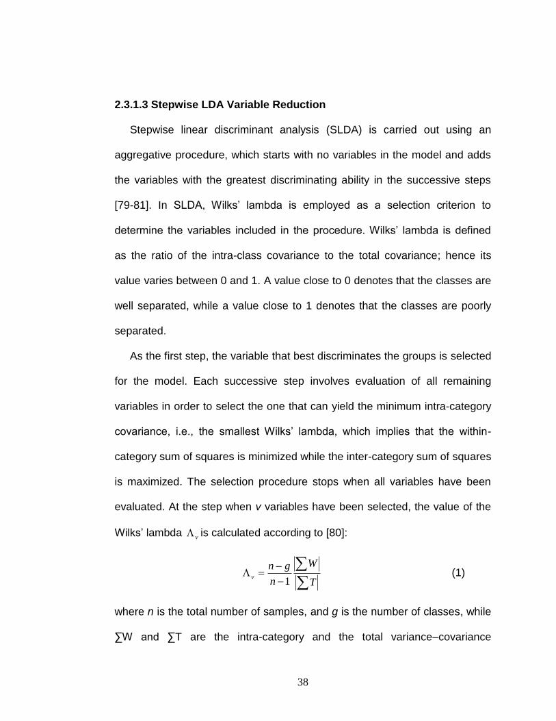
2.3.1.3 Stepwise LDA Variable Reduction
Stepwise linear discriminant analysis (SLDA) is carried out using an
aggregative procedure, which starts with no variables in the model and adds
the variables with the greatest discriminating ability in the successive steps
[79-81]. In SLDA, Wilks‟ lambda is employed as a selection criterion to
determine the variables included in the procedure. Wilks‟ lambda is defined
as the ratio of the intra-class covariance to the total covariance; hence its
value varies between 0 and 1. A value close to 0 denotes that the classes are
well separated, while a value close to 1 denotes that the classes are poorly
separated.
As the first step, the variable that best discriminates the groups is selected
for the model. Each successive step involves evaluation of all remaining
variables in order to select the one that can yield the minimum intra-category
covariance, i.e., the smallest Wilks‟ lambda, which implies that the within-
category sum of squares is minimized while the inter-category sum of squares
is maximized. The selection procedure stops when all variables have been
evaluated. At the step when v variables have been selected, the value of the
Wilks‟ lambda v is calculated according to [80]:
T
W
n
gnv
1 (1)
where n is the total number of samples, and g is the number of classes, while
∑W and ∑T are the intra-category and the total variance–covariance

39
matrices, respectively. Suppose that the Wilks‟ lambda can be approximated
as the F-ratio that follows a Fisher distribution, then the statistical significance
of the changes in lambda is evaluated using the F factor when a new variable
is tested:
1
1
1
v
vv
g
vgnentertoF (2)
where g - 1 and n – g - v are the degrees of freedom for F-to-enter. The new
variable, which is identified to lead to the highest partial F-ratio, i.e., the
largest decrease of the Wilks‟ lambda, is added to the model.
2.3.2 Multivariate Regression Analyses
The aim of computing quantitative models is predicting a property of
unknown samples with spectral data. A model is built and validated by using
several sample sets. A first one is the calibration set used to compute the
model. A second sample set is the validation set used to evaluate the ability
of the model to predict unknown samples. The calibration and the validation
sets have to be independent, and they must consist of samples from different
batches.
2.3.2.1 Multiple Linear Regression
Multiple linear regression (MLR) produces a linear model describing the
relationship between a dependent (response) variable and independent
variables [78, 82]:

40
eXby (3)
where y is the measured response vector ( 1y , 2y , …, ny ), and X is a matrix
of size n × (m + 1) in which the first column are assigned the value 1 as the
intercept term and the remaining columns are assigned the values ijx . The
parameters n, m, i, and j correspond respectively to the number of samples,
the number of variables, the index for samples and the index for variables.
The parameter b is the vector of the estimated regression coefficients, and e
is the vector of the y residuals resulting from systematic modeling errors and
random measurement errors assumed to have normal distribution with
expected value E(e) = 0. By minimizing the sum of the squared residuals, the
regression coefficients can be approximated as [83, 84]:
yXXXb TT 1)( (4)
Each variable jx is then multiplied by its regression coefficient jb to obtain
the predicted value for y, noted as y :
mm xbxbxbby ...ˆ22110 (5)
2.3.2.2 Ridge Regression
MLR is particularly sensitive to highly correlated (co-linear) variables,
which can result in highly unreliable model predictions. In addition, MLR is
inappropriate when there are fewer samples than variables. As a shrinkage
method, Ridge regression (RR) limits the range of the regression coefficients
and thereby stabilizes their estimation [36]. The RR technique aims to resolve

41
the co-linearity problem associated with MLR by modifying the X’X matrix so
that its determinant can be appreciably different from 0. The objective of RR
is to minimize:
m
j
j
n
i
ii byy1
22
1
)ˆ( (6)
where the first term is the residual sum of squares (RSS), and the second
term is a regularizer which penalizes a large norm of the regression
coefficients. The Ridge parameter or complexity parameter λ determines the
deviation between the Ridge regression and the MLR regression, and thereby
controls the amount of shrinkage [83]. As recognized by Equation (4), the
expressions for Ridge regression and MLR are identical when the
regularization parameter λ = 0. The larger the value of λ is, the greater the
penalty (shrinkage) that is applied to the regression coefficients. The Ridge
regression coefficient ridgeb can be estimated by solving the minimization
problem in Equation (6) and has the following form [82, 83]:
yXIXXb TT
ridge
1)( (7)
Equation (7) is a linear function of the response variable y. The coefficient
ridgeb is similar to the regression coefficient of MLR in Equation (4), but the
inverse is stabilized by the Ridge parameter λ. The performance of Ridge
regression depends heavily on proper choice of the parameter λ, which is
achieved using cross-validation procedures.

42
2.3.2.3 Partial Least Squares Regression
Partial least squares regression (PLSR) is one of the most commonly used
multivariate regression methods in chemometrics [36]. The advantage of this
method over multiple linear regression (MLR) is its capacity to build a
regression model based on highly correlated variables. In the model, the X-
data are first transformed into a set of orthogonal latent variables or
components, a linear combination of the original variables, and these new
variables are used for regression with a dependent variable y. The aim of
PLSR is to construct predictive models between two blocks of variables, the
latent variables and the response variables, so that the covariance between
them is maximized. The number of latent variables determines the complexity
of the model and can be optimized by a leave-one-out cross-validation (LOO-
CV) procedure on the calibration set. The relationship between original data X
and the latent variables T is [76]:
ETPX T (8)
Replacing X in the Equation (1) by latent variables T of lower dimension, the
regression model for y on T can be presented as follows [84]:
fTqebPTfbTPeXby T
TT )()( (9)
where T represents the n × r score matrix for X and y, P the m × r loading
matrix representing the regression coefficients of X on T, E the n × m residual
matrix of X, b the m × 1 vector of regression coefficients, q the r × 1 loading

43
vector representing the regression coefficients of y on T, f the n × 1 residual
vector of y, and r is the number of selected factors
2.3.2.4 Support Vector Regression
As a powerful machine learning technique, support vector machine is
becoming increasingly popular. Support vector regression (SVR) is able to
model complex non-linear relationships by using an appropriate kernel
function that maps the input matrix X onto a higher-dimensional feature space
and transforms the non-linear relationships into linear forms. The feature
space is then used as a new input to deal with the regression problem [85].
By introducing an ε-insensitive loss function, Vapnik extended support vector
machines for classification to regression [86, 87]. In the loss function, the
training objects are represented as a tube with radius ε. If all data points are
situated inside the regression tube, the loss function is equal to 0, whereas if
a data point is located outside the tube, the loss function increases with the
Euclidean distance between the data point and the radius ε of the tube [43].
Thus, the ε-insensitive loss function can be expressed as [77, 88]:
,|ˆ|
,0),ˆ,(
ii
iiyy
yyL otherwise
yy ii |ˆ| (10)
A cost function is defined by [83]:
n
i
ii
m
j
j yyLCbI11
2 ),ˆ,(2
1 (11)

44
It is a combination of a 2-norm term of the regression coefficients and an error
term multiplied by the error weight, C, a regularizing parameter which
determines the trade-off between the training error and model complexity [89].
The slack variables i ,
i are introduced for predicting the deviation of more
than ε above ( i ) or less than -ε below (
i ) the target [90], and thus:
)(2
1 *
11
2
i
n
i
i
m
j
j CbI
(12)
Subject to the constraints:
ii
T
i bxby 0
*
0 iii
T ybxb (13)
0, * ii
The Lagrangian is defined as the cost function plus a linear combination of
the above constraints, and the combination coefficients are called the
Lagrange multipliers [83]:
n
i
ii
T
ii
n
i
ii
m
j
j bxbyCbL1
0
1
*
1
2 )()(2
1
*
1
*
11
*
0
* )( i
n
i
i
n
i
ii
n
i
iii
T
i ybxb
(14)
with the Lagrangian multipliers ,0i ,0* i 0i , 0* i for i = 1, …, n. For
training objects with prediction errors smaller than ±ε, their Lagrange
multipliers αi and αi* are zero, while the training objects with prediction errors
larger than ±ε have nonzero αi and αi*, contribute to the final regression

45
model, and are called support vectors. Therefore, the number of support
vectors is determined by the value of ε. The larger the ε value is, the fewer
the support vectors are, and hence the poorer the prediction performance of
the model will be.
A set of values for the Lagrange multipliers can be obtained based on the
Lagrange optimization, and the regression coefficients are expressed as an
expansion of the Lagrange multipliers multiplied by the corresponding training
objects [83]:
ii
n
i
i xb )( *
1
(15)
Thus, the regression model becomes:
0
*
1
)(ˆ bxxXby i
T
ii
n
i
i
(16)
In other words, the response variable can be predicted via the inner products
only, instead of through their individual properties:
TXXXby ˆ (17)
By replacing the inner product TXX with a kernel function ),( ji xxK , this
linear approach can be extended to nonlinear function. For the non-
transformed data set, j
T
i xx is the element ijk . The matrix of element ijk
becomes the inner product of the transformed objects after nonlinear
mapping:
)(),( jiij xxK (18)

46
bxxxxxky j
n
i
jiiiji
n
i
ii )())()()((),()(ˆ1
*
1
*
(19)
where Φ is the mapping function from data X to the feature space.
In support vector regression, there are four typically used kernel functions,
which are linear kernel, polynomial kernel, radial basis function (RBF) kernel,
and sigmoid kernel.
The linear kernel is the inner product of ix and jx :
jiji xxxxK ),( (20)
The polynomial kernel can model nonlinear relationship in a simple and
efficient way:
d
j
T
iji xxxxK )1(),( (21)
RBF is a commonly used kernel, which is usually in the Gaussian form:
)2
exp(),(2
2
ji
ji
xxxxK
(22)
Sigmoid kernel:
)tanh(),( bxaxxxK jiji (23)
2.3.3 Chemometric Pattern Recognition
Chemometric pattern recognition techniques are very powerful in
analyzing multi-dimensional chemical data, and have been widely applied in
such fields as food and pharmaceuticals for identification of their origin,
impurity assessment, and quality control [37, 39, 40, 46]. Chemometric

47
discrimination of different groups is generally divided into two distinct
categories, viz., “unsupervised” (clustering) and “supervised” (classification)
[36, 39]. Unsupervised techniques aim to explore the natural structure of the
data and no information about class membership is required. The most
commonly used methods include principal components analysis (PCA) and
hierarchical cluster analysis (HCA). On the other hand, supervised techniques
focus on defining a classification rule where class membership information
can be used to maximize the separation between groups and the class of a
sample from a test dataset can be predicted based on the mathematical
models derived from the training dataset [37, 38, 91, 92]. The classification of
a collection of samples into groups is usually conducted using supervised
techniques if their origin is known beforehand. Although many pattern
recognition methods are available for classification, the selection of
appropriate methods relies heavily on the specific nature of the data set, such
as the number of classes, samples and variables, the expected complexity of
the boundaries among classes, and the level of noise. While many algorithms
can achieve satisfactory results in typical cases with linear boundaries and
high ratio of samples to variables, the choice of appropriate approaches
should be made carefully in more complicated cases to attain optimal
performance.
Currently, two kinds of supervised pattern recognition methods are
available - pure discriminating approaches and class modeling techniques

48
[79, 93]. The two methods present substantially different modeling strategies
[94]. Discriminating approaches focus on the dissimilarity between classes,
whereas the class modeling techniques emphasize on the similarity within
each class [95]. For pure classification, the training samples are partitioned
into the data space where there are as many regions as the number of
classes, and the classification rule constructs a border among these classes.
A test sample can be only assigned to a specific region or class to which it
most probably belongs. On the other hand, class-modeling analysis considers
only one category at a time and defines a frontier in the feature space to
separate a specific class from the others. A separate mathematical model is
built for each category from a training set, and then the fitting of samples is
evaluated. A sample is accepted by that class if it falls within a model‟s space,
whereas it is considered an outlier for that specific class if it falls outside the
model‟s space. If more than a single class is modeled, a particular region of
the data space from one class may overlap within the boundaries of other
class models. Therefore, a sample can be assigned to a single class, to more
than one class, or to none of the classes [93]. In chemometrics, the most
commonly used class-modeling tools are soft independent modeling of class
analogy (SIMCA) [96-98] and unequal class modeling (UNEQ, also known as
multidimensional Gauss class modeling or MGCM) [80, 93, 95, 99], which are
distance- and probabilistic-based modeling techniques, respectively. As a

49
modeling version of quadratic discriminant analysis (QDA), UNEQ is the
simplest modeling method based on multivariate normal distribution [79, 94].
An NMR data-analysis procedure is shown in the Figure 6 [100]. After
spectra are accumulated and processed (panel a), a primary data reduction is
carried out that digitizes the one-dimensional spectrum into a series of
integrated regions (panel b). After removal of redundant signals and
appropriate scaling, primary data analysis is used to map the samples
according to their composition and property, using methods such as PCA.
Samples that share a similar property are generally intrinsically similar in
composition, and therefore occupy neighboring positions in the PC space
(panel c). Each class of samples is then modeled separately, and class
boundaries and confidence limits are calculated to construct a model for the
prediction of independent data (panel d).
Figure 6. Schematic diagram representing the process of assessing sample class from raw NMR spectra. Taken from Ref [100].
50
2.3.3.1 Principal Components Analysis
As a well-established multivariate statistical technique, principal
components analysis (PCA) is able to determine the directions of greatest
variance in the dataset, to reduce the dimensionality of the dataset where
there are a large number of intercorrelated variables, and to simplify complex
datasets to generate a lower number of parameters while retaining as much
as possible of the information present in the original data [44-46, 101]. PCA
clusters samples into separate groups in n-dimensional space, where “n” is
the number of features or variables that characterizes each sample. PCA is
especially useful as a discovery tool for complex multivariate data sets,
because this approach reduces the original variables to a much smaller set
that greatly simplifies visualization of the data to see hidden patterns and
similarities/ dissimilarities between the clusters.
PCA approach transforms the original correlated variables into the
uncorrelated ones known as principal components (PC), which are a linear
combination of the original variables and are orthogonal to each other. The
first component explains the maximum amount of variance in the data, and
each succeeding component accounts for the remaining variations. PCA is an
unsupervised method in that no a priori knowledge relating to class affiliation
is required [102]. PCA is commonly used to visualize samples as scores plots
of two dimensions (PC1 vs PC2) or three dimensions (PC1 vs PC2 vs PC3)
that exhibit the number of distinct clusters and the differences between

51
clusters in terms of their characteristic location in variable space. PCA has
been widely applied in conjunction with various discriminant analysis
techniques to handle classification problems. In addition, the PC scores can
be used as inputs to multivariate analyses [103, 104]. In PCA analysis, the
data matrix X is composed of the product of PCA scores matrix T and loading
matrix P plus the error or residual matrix E [77]:
ETPX (24)
2.3.3.2 Partial Least Squares Discriminant Analysis
Partial least squares discriminant analysis (PLS-DA) is a linear regression
approach in which the multivariate variables from the observations are
correlated to the class membership of each sample [41, 105-107]. As an
extension of PCA, PLS-DA attempts to build models that can maximize the
separation among classes of objects. Since the class affiliation of the objects
is included in the regression calculation, PLS-DA is a supervised approach.
PLS-DA models the dataset in a way similar to PCA, but with the addition of
discriminant analysis. Unlike PCA which focuses on the overall variation of
each class, PLS-DA focuses mainly on the variation between classes.
There are two steps for the PLS-DA procedure [42, 103, 108]: the first one
is the application of a PLS regression model on the latent variables which
indicates the grouping information, and the second one is classification of the
objects from the regression results on indicator variables. Once built and
52
validated, a PLS-DA model can be used to predict the class membership for
unknown samples.
The regression of the data (X) against a “dummy matrix” (Y) describes the
variation according to class affiliation, where Y contains the values of 1 and 0
for each class and consists of as many columns as there are classes [35]. For
the training set, an observation is assigned the value of 1 for its class
affiliation, and assigned 0 for the other classes. The output of PLS-DA
regression is a matrix which can be used to classify unknown samples. The
prediction result from the PLS-DA model is a numeric value. If the value is
close to 1, then the test sample is assigned to the modeled class; if the value
is close to 0, then the object is unassigned or assigned to another class.
2.3.3.3 Linear Discriminant Analysis
Linear discriminant analysis (LDA) is a widely used supervised pattern
recognition method, and is also a well-established dimension reduction
technique [103, 109]. In LDA, a linear function of the dataset is sought so that
the ratio of between-class variance is maximized and the ratio of within-class
variance is minimized, and finally the optimal separation among the given
classes is achieved. Like PLS-DA, the ultimate aim of LDA is to qualitatively
predict the group affiliation for unknown samples. Discrimination of the
classes is performed by calculating the Mahalanobis distance of a sample
from the center of gravity of each specified class, and then assigning the
sample to the class associated with the smallest distance [103, 110]. The

53
Mahalanobis distance between a sample ( ix ) and the data center ( x ) is
defined as [111]:
5.01 )]()()[()( xxXXxxxD i
TT
ii (25)
where 1)( XX T is the sample covariance matrix and i denotes the index of
samples. The center is estimated by the arithmetic mean vector x . A test
sample is correctly classified if it is located nearest the center of gravity of its
actual class. Otherwise, the sample would be incorrectly classified to another
class for which the Mahalanobis distance was the smallest.
2.3.3.4 k-Nearest Neighbors
The classification of k-nearest neighbors (kNN) is performed by calculating
the distances between a new object (a test data point) and all objects in the
training set in n-dimensional variable space [112, 113]. Unlike PLS-DA and
LDA, the kNN approach avoids the need for model generation. Neighbor
determination is calculated by the Euclidean distance, and the nearest k
objects were used to estimate the class affiliation of the test object. Euclidean
distance is expressed as [36]:
m
j
jiji xxxxD1
5.02
, ])([),( (26)
where i and j denote the index of samples and variables, respectively, and m
is the number of variables. By applying the majority rule, the new object is
assigned to the class of the majority of the k objects, i.e., the prediction is
related to a majority vote among the neighbors. To correctly assign the group

54
affiliation for a test data point, this technique requires tuning of the adjustable
parameter k (i.e., the optimal number of nearest neighbors to choose). Values
of k that are too small or too large can lead to poor classification of new
objects. Over-fitting may occur if k is too small (such as k = 1), while under-
fitting is more likely if k is too large. By testing a series of k values and
assessing the prediction performance, the optimal value of k is selected which
gives the lowest number of misclassifications.
2.3.3.5 Classification and Regression Tree
As a non-parametric approach, classification and regression tree (CART)
models a data set with the structure of a tree and makes no assumption about
the distribution of the data. This methodology applies decision trees to solve
classification and regression problems for handling both categorical and
continuous responses. A classification tree is yielded when the response
variable is categorical, while the final output is a regression tree when the
response variable is continuous. In general, a CART analysis consists of
three steps [114-117]: in the first step, an over-large tree, called the maximal
tree, is built by recursive partitioning of the original training data using a
binary split-procedure; in the second step, the overgrown tree, which usually
shows overfitting, is pruned so that a series of less complex trees is derived;
in the last step, the tree with the optimal size is selected by a cross-validation
(CV) procedure.

55
The tree construction starts by dividing the root node, containing all
objects in the training set, into exactly two sub-groups or child nodes, and
then each child node becomes a parent node that is further split into two
mutually exclusive child nodes. The splitting procedure is repeated for each of
the resulting nodes until the maximal tree is grown, which is defined as the
tree in which each terminal node consists of either just one object, or contains
a predefined number of objects, or all objects contained in the node are as
pure or homogeneous as possible, i.e., the samples in a node share the same
or similar values of the response variable (Figure 7). To find the most
appropriate variable for splitting and the best split point on the variable so that
the error measure is minimized or the predictive power is maximized, CART
scans through all possible split values over all explanatory variables. In the
decision tree, the first branch is produced by the variable with the best split
point, and each sequential split is conducted by following some fit criteria or
error measures Ql(T) with the purpose of decreasing the misclassification as
much as possible. For classification trees to choose the best split point,
several splitting criteria have been proposed, one of them being the Gini
index which represents the product sum of the relative frequency of one class
and the relative frequency of all other classes, and can be expressed as [36]:
)1()1(11 l
ljk
j l
ljk
j
ljljn
n
n
nppGini
(27)

56
where k denotes the number of possible classes; nl is the number of objects
in node l, and nlj is the number of objects from class j present in the node l.
When the node is pure, i.e., contains only objects of the same group, the
minimum Gini index value is attained.
Figure 7. Structure of a classification or regression tree. Nodes 1, 3 and 4 are TNs, node 2 is a parent node, and nodes 3 and 4 are child nodes. Taken from Ref [114].
The tree built in the first step fits the training set almost perfectly, but
usually exhibits poor predictive ability for new samples, because it has a large
number of terminal nodes (TNs). It is necessary to find trees with less
complexity but better predictive accuracy. The optimal tree size can be
determined by successively cutting back the terminal branches of the
overlarge tree. During this pruning procedure, a series of smaller sub-trees T
are derived from the maximal tree, and the optimal tree with the minimum

57
classification error is obtained by calculating its cost-complexity parameter
CPα(T) as a measure, which is defined as a linear combination of the tree
cost Ql(T) and its complexity |T| [36]:
Minimize: TTQnTCPT
l
ll 1
)()( (28)
where |T| denotes the size of a tree, or the number of terminal nodes, i.e., the
complexity of the sub-tree T; and α, which takes values between 0 and 1, is a
penalty for each additional terminal node, and it establishes the compromise
between classification error and tree size. For each value of α, the optimal
tree size is selected by minimizing CPα(T). A value of α equal to zero results
in the maximal tree where the measure Ql(T) of misclassification is minimized
while the value α > 0 penalizes large trees. By gradually increasing the value
of α starting from 0, a nested sequence of trees with decreasing size or
complexity is then derived. The last stage of this procedure is to compare the
different sub-trees and select the optimal tree from the remaining sequence of
sub-trees, which is determined by cross validation for evaluation of the
predictive error.
2.3.3.6 Artificial Neural Networks (ANNs)
An aritificial neural network (ANN) is a well-established modeling
technique for solving some problems such as classification or pattern
recognition, regression and estimation [37, 38, 91, 92, 118-122]. ANN is able
to handle linear as well as non-linear data for model fitting, and consequently

58
it excels in cases where the data sets contain substantial uncertainty and
measurement errors. ANN is particularly suitable when a mathematical
relationship between the independent and response variables cannot be
established. The typical feed-forward back-propagation ANN is composed of
a large number of fully interconnected processing elements (PE) or neurons
which are organized into a sequence of layers (Figure 8).
Figure 8. A fully connected multilayer feed-forward back-propagation network. Taken from Ref [122].
The first layer is the input layer that contains as many neurons as the
number of independent variables and is used to receive the information from
the outside. The last layer is the output layer consisting of as many neurons
as the number of dependent variables and serves to provide ANN‟s response
to the input data. A series of one or more hidden layers are in between, which
are responsible for communicating with the neurons of the input and output

59
layers. A number of learning algorithms are available for training a neural
network. For multilayer ANNs, the most commonly used approach is the
single hidden layer network with a sufficient number of neurons, which can
model any nonlinear function with any required accuracy. In a feed-forward
architecture, signals are propagated sequentially only in the forward direction,
i.e., from the input layer through the hidden layer to the output layer, where
the output from a previous layer is employed as an input for the successive
layer.
The propagation of the signal through the network from one neuron in a
layer to another neuron in the next layer greatly depends on the strength of
the connection. The interconnections between neurons are represented by a
set of adjustable parameters called weights that are calculated by the ANN
algorithm, which trains the neural network and adapts the weights to an
optimum set of values. In the training process, some interconnections are
strengthened while the others are weakened, in such a way that the ANN will
yield more accurate results. As a popular learning strategy, back propagation
approach corrects the weights in a layer, which are proportional to the error
from the previous layer. The prediction results are fed backwards through the
network to adjust the weights. This process is repeated until the
interconnections are optimized, the error is minimized, the trained network
attains a specified level of accuracy, or a pre-defined number of iterations are
reached.

60
The activation of the neuron is done through the weighed sum of the
inputs, and a transfer function is used to pass the activation signal and
produce a single output of the neuron. The relationship between the input
variable xi and the output variable y is defined by the following equation
formula [118]:
j i jiiijj bbxwfwfy ])([ (29)
where wij and wj represent the connection weights from the input layer to the
hidden layer and from the hidden layer to the output layer, respectively, and bi
and bj are bias constants. The transfer function f(x), which can be linear or
non-linear depending on the topology of the network, determines the
processing inside the neuron. The logistic sigmoid activation function is a
widely used transfer function:
xe
xf
1
1)( (30)
2.3.3.7 Support Vector Machine (SVM)
Support vector machine (SVM) is a recently developed modeling
technique that has demonstrated its utility for a broad range of classification
and regression problems [88, 123-133]. SVM performs pattern recognition by
finding an optimal hyperplane as the decision boundary for separating two
classes of patterns, which can maximize the margin between the closest data
points of each class. The SVM algorithm derives the classification rule using
only a fraction of the training samples that are known as support vectors

61
(SVs) and typically are situated nearby on the margin borders. In general, the
number of SVs is much lower than the number of training samples. For the
linearly separable case, the class boundary is determined in the space of the
original variables by defining an optimal hyperplane with maximal margin,
which divides the data-space into two regions with opposite sign, and leaves
all the vectors of the same sign or class on the same side [123, 124]:
0 bxwT (31)
where w is a weight vector normal to the hyperplane, b is a free threshold
parameter, b/||w|| is the perpendicular distance to the origin, and ||w|| is the
Euclidean norm of w. In linearly non-separable situations, the principle of
linear separation is extended and the complex class boundaries are modeled
by using adequate kernel functions that map the original vectors from input
space to higher dimensional feature space where the non-linear relationship
is expressed in linear form and a linear separation operation can be
performed (Figure 9).
Figure 9. Non-linear separation case in the low dimension input space and linear separation case in the high dimension feature space. Taken from Ref [126].

62
In the presence of noisy data, the learned classifier may fit the noise into
model and force zero training error, leading to poor generalization. The
violation of the margin constraints of the hyperplane is allowed by introducing
a set of non-negative slack variables ξi > 0 (i = 1, . . ., n), which represents
the distance of sample xi from the margin of the pertaining class. Given the
sum of the allowed deviations ∑ξi, the optimization requires simultaneously
maximizing the margin 1/2||w||2 and minimizing the number of
misclassifications. Accordingly, the objective function that is designed to
balance the classification error with complexity of the model can be
expressed as following [88]:
n
i
iCw1
2
2
1 (32)
A soft margin that can separate the hyperplane is constructed by minimizing
the dual form of the above expression, where the regularization parameter C
is used to control a trade-off between maximizing the margin and minimizing
the model complexity. A small value of C allows great deviations ξi, and
hence, the emphasis will be placed on margin maximization and a large
number of samples are retained as support vectors, leading to overfitting of
the training data. In contrast, when C is too large, the second term dominates,
allowing smaller deviations ξi and minimizing the training error, leading to a
less complex boundary and smaller margin.

63
The results of the SVM approach depend highly on the choice of the
kernel function that decides the sample distribution in the mapping space and
may influence the performance of the final model. The most commonly used
kernel function in SVM is radial basis function (RBF) or Gaussian function,
and is formulated as [125]:
)exp(),(2
jiji xxxxK (33)
where xi and xj are two independent variables; γ is a tuning parameter that
controls the amplitude of the kernel function and, therefore, controls the
generalization performance of the SVM. A very large γ value can produce
models with overfitting because most of the training objects are used as the
support vectors, while a very small γ value can lead to poor predictive ability
as all data points are regarded as one object.
2.3.3.5 SIMCA Analysis
Soft independent modeling of class analogy (SIMCA) is a widely applied
class modeling technique in chemometrics. SIMCA uses the principal
component analysis (PCA) to develop a statistical model which describes the
similarities among the samples of a category [79, 134, 135]. The class model
for each category is derived separately in the training set based on the
computation of the principal components (PCs). The number of significant
components, which determines the dimensionality of the inner space for each
category and can differ for each category, is evaluated by a cross validation

64
procedure. Depending on the number of PCs or the variance retained in each
data class, classes can be modeled by one of a series of linear structures,
such as a point, a line, a plane, and so on [36]. In the space of the first few
PCs, the SIMCA model exhibits a parallelepiped structure, delimited by the
range of the scores in the direction of each PC.
The class boundaries around these linear structures can be built on the
basis of the distribution of Euclidean distance between the data points of
training samples and the fitted class model. The mean distance between the
samples belonging to a class and the class model, i.e., the class residual
standard deviation 0s , is defined as [136]:
)]1)(/[(1 1
22
0
AnAmesn
i
m
j
ij (34)
where n, m and A denote the number of samples in the class, the number of
variables, and the number of categories, respectively, and 2
ije is the squared
residual of the ith sample for the jth variable. A critical distance crits is
computed based on an F-test at a certain limit of confidence level:
critcrit Fss 0 (35)
In the present study, a 95% confidence level was set to define each class.
After the model has been developed on the training set, a new sample can be
tested for its membership in the defined classes by the orthogonal projection

65
distance between the new sample and the PC model of each class. The
squared distance of the test sample is determined by:
)/(1
2
,
2 Amesm
j
jtesttest
(36)
It is then compared with the class confidence limit crits . The new sample is
assigned to one or more classes if it lies within the statistical limits, i.e.,
tests < crits , and it is considered to be an outlier if the distance is larger [79].
Therefore, a sample can be a member of a single class, more than one class,
or none of the defined classes.
The model generated by SIMCA for each category can be evaluated in
terms of sensitivity (SENS) and specificity (SPEC), which are associated with
the number of false positive and false negative errors for each class. The
SENS of a class is the proportion of samples belonging to that class and
correctly identified by the model, while SPEC corresponds to the proportion of
samples outside the class and correctly rejected by the model [95, 135, 137].
When more than two classes are present, specificity can be calculated
individually for each class. SENS and SPEC are closely associated with the
concepts of type I (α) errors which refer to the probability of erroneously
rejecting a member of the class as a non-member (false negative), and type II
(β) errors which refer to the probability of erroneously accepting a non-
member of the class as a member (false positive). Assume An and An are
the number of samples belonging to category A and the number of samples

66
accepted by the model, respectively, while An and An are the number of
samples not belonging to category A and the number of samples rejected by
the model, respectively. Given these definitions [85], the two relationships
follow:
100A
A
n
nSENS (37)
100A
A
n
nSPEC (38)
indicating that SENS and SPEC are the complementary percent measure of
type I and II errors, respectively.
2.3.3.6 UNEQ Analysis
UNEQ is a class-modeling technique equivalent to quadratic discriminant
analysis (QDA) and is based on the assumption of multivariate normal
distribution of the measured or transformed variables for each class
population [79, 94, 95]. In this method, each category is represented by
means of its centroid.
In a specific class, the category space or the distance of each sample from
the barycenter or centroid is calculated according to various measures that
follow a chi-squared distribution. Usually, the Mahalanobis distance is
applied, which is measured on the basis of correlations between variables
and is a useful way for determining similarity of an unknown sample set to a
known one. The Mahalanobis distance is different from Euclidean distance in
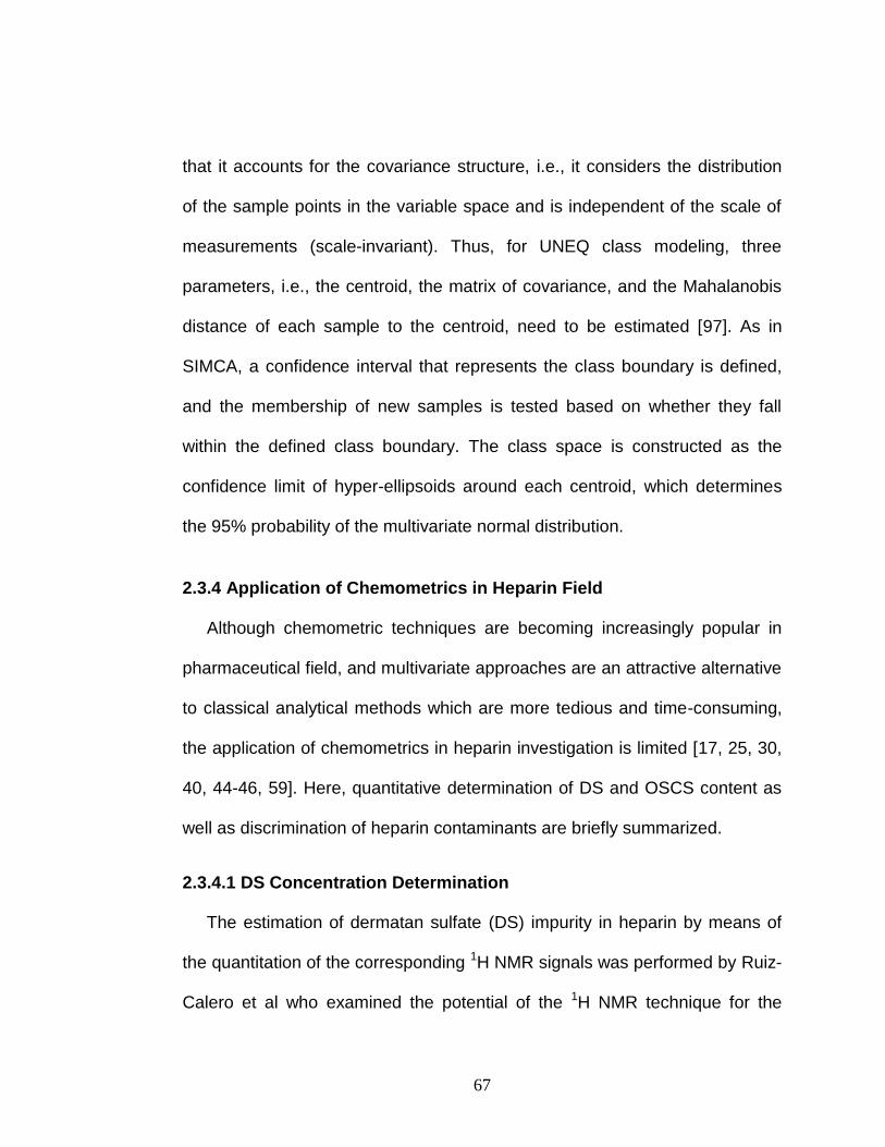
67
that it accounts for the covariance structure, i.e., it considers the distribution
of the sample points in the variable space and is independent of the scale of
measurements (scale-invariant). Thus, for UNEQ class modeling, three
parameters, i.e., the centroid, the matrix of covariance, and the Mahalanobis
distance of each sample to the centroid, need to be estimated [97]. As in
SIMCA, a confidence interval that represents the class boundary is defined,
and the membership of new samples is tested based on whether they fall
within the defined class boundary. The class space is constructed as the
confidence limit of hyper-ellipsoids around each centroid, which determines
the 95% probability of the multivariate normal distribution.
2.3.4 Application of Chemometrics in Heparin Field
Although chemometric techniques are becoming increasingly popular in
pharmaceutical field, and multivariate approaches are an attractive alternative
to classical analytical methods which are more tedious and time-consuming,
the application of chemometrics in heparin investigation is limited [17, 25, 30,
40, 44-46, 59]. Here, quantitative determination of DS and OSCS content as
well as discrimination of heparin contaminants are briefly summarized.
2.3.4.1 DS Concentration Determination
The estimation of dermatan sulfate (DS) impurity in heparin by means of
the quantitation of the corresponding 1H NMR signals was performed by Ruiz-
Calero et al who examined the potential of the 1H NMR technique for the
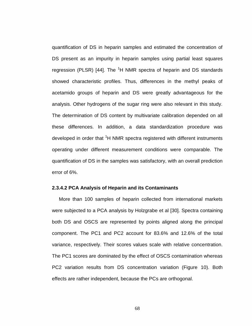
68
quantification of DS in heparin samples and estimated the concentration of
DS present as an impurity in heparin samples using partial least squares
regression (PLSR) [44]. The 1H NMR spectra of heparin and DS standards
showed characteristic profiles. Thus, differences in the methyl peaks of
acetamido groups of heparin and DS were greatly advantageous for the
analysis. Other hydrogens of the sugar ring were also relevant in this study.
The determination of DS content by multivariate calibration depended on all
these differences. In addition, a data standardization procedure was
developed in order that 1H NMR spectra registered with different instruments
operating under different measurement conditions were comparable. The
quantification of DS in the samples was satisfactory, with an overall prediction
error of 6%.
2.3.4.2 PCA Analysis of Heparin and its Contaminants
More than 100 samples of heparin collected from international markets
were subjected to a PCA analysis by Holzgrabe et al [30]. Spectra containing
both DS and OSCS are represented by points aligned along the principal
component. The PC1 and PC2 account for 83.6% and 12.6% of the total
variance, respectively. Their scores values scale with relative concentration.
The PC1 scores are dominated by the effect of OSCS contamination whereas
PC2 variation results from DS concentration variation (Figure 10). Both
effects are rather independent, because the PCs are orthogonal.

69
Figure 10. Scores plot of the PCA analysis for the
1H NMR spectral data of heparin
samples containing DS and OSCS. Taken from Ref [30].
Beyer et al [17] conducted PCA analysis of qualitative characteristics of
heparin samples in order to evaluate whether these contaminants are related
to each other. The existence of the various contaminants was represented by
the encoding scheme: -1 is used when the contaminant was not detected
while +1 encoded the contaminant. The application of the PCA revealed that
the samples containing OSCS can be separated from all other samples by
plotting the scores of PC3 against the scores of PC4 (Figure 11).
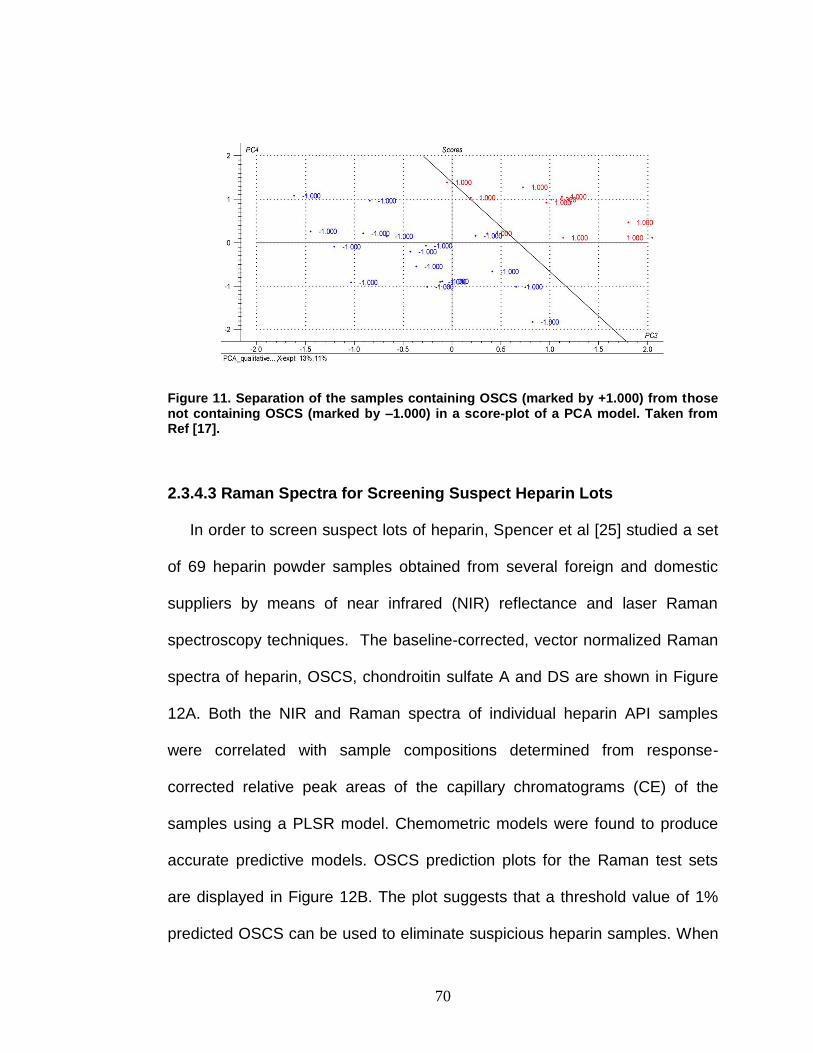
70
Figure 11. Separation of the samples containing OSCS (marked by +1.000) from those not containing OSCS (marked by –1.000) in a score-plot of a PCA model. Taken from Ref [17].
2.3.4.3 Raman Spectra for Screening Suspect Heparin Lots
In order to screen suspect lots of heparin, Spencer et al [25] studied a set
of 69 heparin powder samples obtained from several foreign and domestic
suppliers by means of near infrared (NIR) reflectance and laser Raman
spectroscopy techniques. The baseline-corrected, vector normalized Raman
spectra of heparin, OSCS, chondroitin sulfate A and DS are shown in Figure
12A. Both the NIR and Raman spectra of individual heparin API samples
were correlated with sample compositions determined from response-
corrected relative peak areas of the capillary chromatograms (CE) of the
samples using a PLSR model. Chemometric models were found to produce
accurate predictive models. OSCS prediction plots for the Raman test sets
are displayed in Figure 12B. The plot suggests that a threshold value of 1%
predicted OSCS can be used to eliminate suspicious heparin samples. When

71
the NIR model is used, a 1% threshold resulted in 38 out of 41 samples
correctly classified as being either good (15 samples at OSCS < 1%) or
suspect (26 samples > 1% OSCS). One good sample was classified as
suspect (1 false negative) and one suspect sample was classified as good
(false positive). Prediction with the Raman model showed similar accuracy,
with 36 out of 38 samples being correctly classified with one false positive
and one false negative. The overall accuracy in classifying heparin samples
as suspect or good using these spectroscopic/chemometric methods as
screening tools can be expected to exceed 95%. Both NIR and Raman allow
the elimination of over 60% of the heparin samples as suspicious. The
remaining 40% would be subjected to additional analyses by CE, NMR or
other separation methods to detect the presence of low levels of OSCS.
A B
Figure 12. Comparison of Raman spectra of heparin and the principal contaminants (A) and Raman PLS model test for OSCS of thirty eight samples (B). Solid diamond points are considered ‘‘Good’’; open square points are ‘‘Suspect’’. Taken from Ref [25].

72
Chapter III
DATA AND METHODS
In the present study, all 1H NMR spectral data were provided by the
Division of Pharmaceutical Analysis (DPA) of the US FDA, and various
multivariate regression approaches as well as pattern recognition techniques
were applied to the data.
3.1 Heparin Samples
Over 200 heparin sodium API samples from different manufacturers and
suppliers were analyzed. These samples contained substantial amounts of
DS (up to 19% of the polymer mixture) and OSCS (in an amount from 0 to
27%).
3.1.1 Pure, Impure and Contaminated Heparin APIs for Classification
Preliminary screening of heparin batches collected from different sources
by means of 1H NMR spectroscopy and capillary electrophoresis (CE)
revealed four different groups, i.e., pure heparin with DS ≤ 1.0%, heparin
containing DS in varying amounts but without OSCS, heparin with OSCS and
without DS, and heparin with both OSCS and DS.
Revisions proposed by the FDA for the Stage 3 Heparin Sodium USP
monograph specify that the weight percent of galactosamine in total

73
hexosamine (%Gal) may not exceed 1.0% and no level is acceptable for
OSCS. Thus, the samples in this study were divided into three groups: (a)
pure heparin with DS ≤ 1.0% and OSCS = 0% (Heparin); (b) impure heparin
with DS > 1.0% and OSCS = 0% (DS); and (c) contaminated heparin with
OSCS > 0% and any content of DS (OSCS). An additional fourth class,
namely [DS + OSCS], was included to characterize samples that contained
DS > 1.0%, OSCS > 0%, or both. In order to obtain a model with validation
capabilities, data was divided into two data sets: a training set employed to
build the model, and a validation set employed to test the predictive ability of
the model using data excluded from the training set. The data set of 178
heparin samples was split 2:1 into 118 samples for training (54 Heparin, 33
DS, and 31 OSCS) and 60 samples for external validation and testing (28
Heparin, 17 DS, and 15 OSCS). Multivariate statistical modeling was
conducted separately on the entire region (1.95-5.70 ppm) and two local
regions (1.95-2.20 and 3.10-5.70 ppm), which correspond to 74, 9 and 65
variables, respectively.
3.1.2 Heparin API Samples for %Gal Determination
1H NMR analytical data of over 100 heparin sodium API samples from
different suppliers with varying levels of chondroitins were obtained from the
chromatographic and spectroscopic experiments. DS is the primary
chondroitin impurity observed in heparin APIs and, for the purpose of this
study, the %Gal is presumed to be the same as the %DS for samples not

74
containing OSCS. These samples contained up to 10% by weight of
chondroitins in the API by the %Gal HPLC assay. Based on the range of
%Gal, the NMR spectral data were classified into two datasets, Dataset A and
Dataset B, which correspond to 0-10% and 0-2% galactosamine, respectively,
so Dataset B is a subgroup of Dataset A. For each dataset, heparin samples
were randomly split into two subsets: a training set that is used to build the
calibration models and an independent test set that is used to evaluate and
validate the model‟s predictive ability. The statistics of these two datasets are
summarized in Table 1. In the present study, models built by Dataset A and
Dataset B are named Model A and Model B, respectively.
Table 1. Summary Statistics of %Gal Measured from HPLC __________________________________________________________________________________
Number of samples Minimum Maximum Median Mean __________________________________________________________________________________
Dataset A
Training set 76 0.01 9.68 0.86 1.74
Test set 25 0.11 8.05 0.87 1.76
Dataset B
Training set 57 0.01 1.86 0.66 0.71
Test set 19 0.11 1.74 0.72 0.73 __________________________________________________________________________________
3.1.3 Blends of Heparin Spiked with other GAGs
A series of blends was prepared by spiking heparin APIs with native
impurities chondroitin sulfate A (CSA), chondroitin sulfate B (CSB, or DS),
heparan sulfate (HS), or synthetic contaminants oversulfated-(OS)-CSA (i.e.,

75
OSCS), OS-CSB, OS-HS or OS-heparin at the 1.0%, 5.0% and 10.0% weight
percent levels [15]. The detailed composition of the series of blends is
reported in the Chapter VI: Results and Discussion.
3.2 Proton NMR Spectra
Figure 13 illustrates the overlaid 500 MHz 1H NMR spectra of heparin
samples that contained 10.0% weight percent spikes of native and synthetic
GAGs, i.e., chondroitin sulfate A (CSA), oversulfated CSA (OS-CSA or
OSCS), chondroitin sulfate B (CSB) or dermatan sulfate (DS), and
oversulfated CSB (OS-DS), plotted in the range from 1.95 to 6.00 ppm. The
methyl protons of the N-acetyl methyl groups resonated around a chemical
shift of ca. 2 ppm, which was well separated from the other NMR signals in
the 3.0 to 6.0 ppm range where a complex pattern of overlapping signals
occurred. Each spectrum revealed distinctive features, and their respective
patterns were easily distinguished from one other in the range from 1.95 to
2.20 ppm (Figure 13A). The basic repeating disaccharide unit for heparin is 2-
O-sulfated uronic acid and 6-O-sulfated N-sulfated glucosamine, whereas the
corresponding repeating unit for DS or OSCS is uronic or glucuronic acid,
respectively, and galactosamine. About every fifth amino group is acetylated
for heparin, but almost all of the amino groups are acetylated in DS and
OSCS [21, 30]. A single peak appeared at 2.05 ppm for the N-acetyl protons
of heparin, and the methyl signal shifted about 0.03 ppm downfield in DS.

76
A
B
Figure 13. An overlay of the 500MHz
1H NMR spectra of a heparin sodium API spiked
with 10.0% weight percent of CSA, OS-CSA, DS and OS-DS. (A) In the 2.20-1.95 ppm region; (B) In the 6.00-3.00 ppm region.

77
Thus, a small peak, corresponding to the N-acetyl protons of DS, was
observed near 2.08 ppm. For OS-DS, two signals, which were located at 2.09
and 2.11 ppm, appeared downfield of the heparin methyl signal. A shoulder
peak at 2.02 ppm appeared upfield of the heparin methyl proton signal for
CSA while OS-CSA exhibited a characteristic signal near 2.15 ppm. Figure
13B showed the 3.0-6.0 ppm region of the overlaid spectra. The presence of
CSA resulted in the signals at 3.38, 3.58 and 4.02 ppm while the
characteristic peaks at 4.16, 4.48, 4.97 and 5.01 ppm came from OS-CSA.
DS displayed resonances at chemical shifts distinct from those of heparin at
3.54, 3.87, 4.03, 4.68 and 4.87 ppm. In addition, the signals at 4.27 and 4.93
ppm were associated with the OS-DS sample.
The proton NMR spectra of heparin samples are rich in information.
Although it is difficult to assign all peaks in the spectrum for use in the
determination of the quality of complex APIs such as heparin, these patterns
of intensities are valuable for characterizing and quantifying analytes for
quality control and purity assessment [39], and ideal for analysis using
chemometric approaches.
3.3 Data Processing
Prior to building multivariate models, the 1H NMR spectra of the heparin
samples were preprocessed into a discrete set of variables that served as the
input to the pattern recognition tools for subsequent analysis of the pure, DS-
impure, and OSCS-contaminated heparin samples.

78
1H NMR spectra were processed using the software MestRe-C (Version
5.3.0). Phase correction was achieved through automatic zero- and first-order
correction procedures, and peak integration was performed for each spectral
region. Chemical shifts were referenced to internal 4, 4-dimethyl-4-
silapentane-1-sulfonic acid (DSS). For the chemometric analysis, each 1H
NMR spectrum was automatically data-reduced and converted into 125
variables by dividing the 1.95 to 5.70 ppm region into sequential windows with
width of 0.03 ppm. During initial processing of the data, heparin lots were
found to contain residual solvents and reagents such as ethanol (triplet at
1.18 and quartet at 3.66 ppm), acetate (singlet at 1.92 ppm), and methanol
(singlet at 3.35 ppm) at varying levels. In addition, the residual H2O in the D2O
had a strong signal at 4.77 ppm. These regions were excluded from the data
acquisition, and the total data set was reduced to 74 regions or variables,
which are listed in Table 2 together with their corresponding chemical shifts.
The area within the spectral regions was integrated. In order to
compensate for differences in concentration among the heparin samples, the
74 variables for each spectrum were normalized to the total of the summed
integral value. Prior to chemometric analysis, the spectra were converted into
ASCII files where the data were represented in n × m-dimensional space (n
and m equal to the number of samples and the number of variables,
respectively), and the resulting data matrix was imported into Microsoft Excel
2003. The data were preprocessed by autoscaling, also known as unit
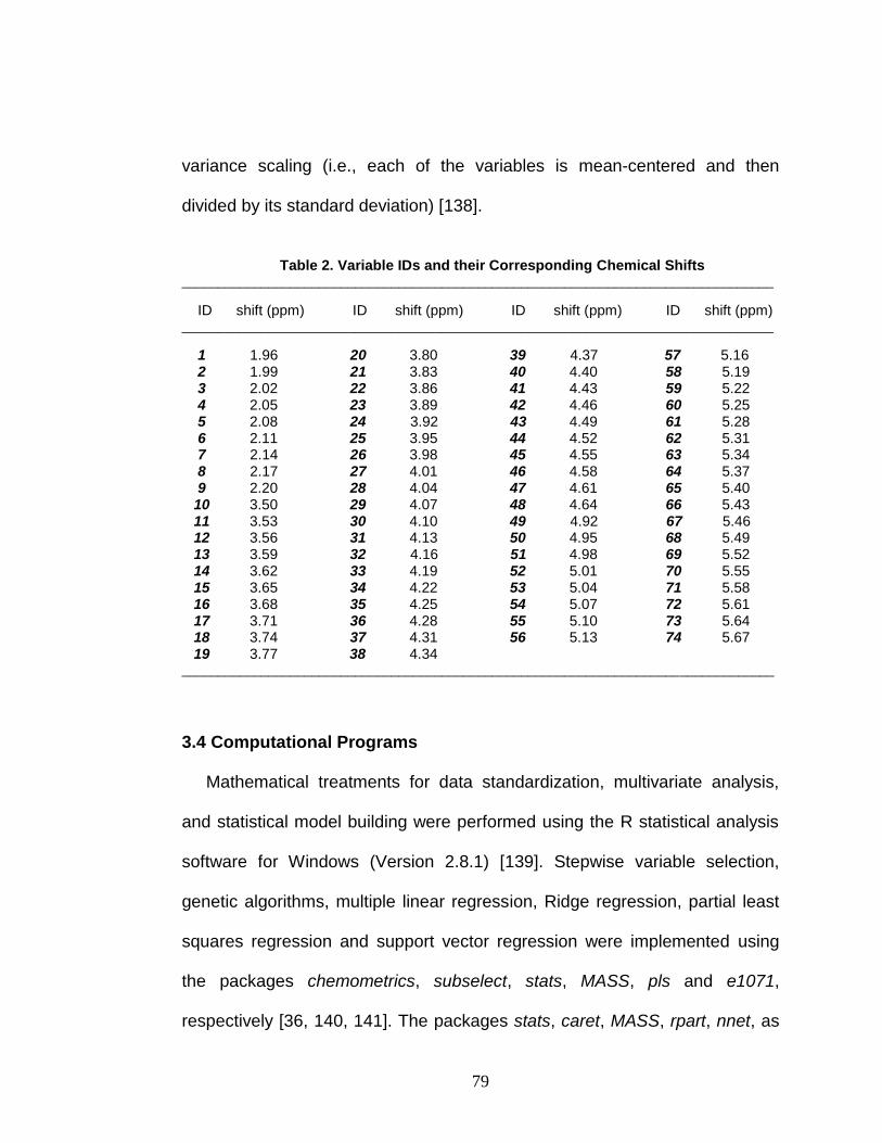
79
variance scaling (i.e., each of the variables is mean-centered and then
divided by its standard deviation) [138].
Table 2. Variable IDs and their Corresponding Chemical Shifts __________________________________________________________________________________
ID shift (ppm) ID shift (ppm) ID shift (ppm) ID shift (ppm) __________________________________________________________________________________
1 1.96 20 3.80 39 4.37 57 5.16 2 1.99 21 3.83 40 4.40 58 5.19 3 2.02 22 3.86 41 4.43 59 5.22 4 2.05 23 3.89 42 4.46 60 5.25 5 2.08 24 3.92 43 4.49 61 5.28 6 2.11 25 3.95 44 4.52 62 5.31 7 2.14 26 3.98 45 4.55 63 5.34 8 2.17 27 4.01 46 4.58 64 5.37 9 2.20 28 4.04 47 4.61 65 5.40 10 3.50 29 4.07 48 4.64 66 5.43 11 3.53 30 4.10 49 4.92 67 5.46 12 3.56 31 4.13 50 4.95 68 5.49 13 3.59 32 4.16 51 4.98 69 5.52 14 3.62 33 4.19 52 5.01 70 5.55 15 3.65 34 4.22 53 5.04 71 5.58 16 3.68 35 4.25 54 5.07 72 5.61 17 3.71 36 4.28 55 5.10 73 5.64 18 3.74 37 4.31 56 5.13 74 5.67 19 3.77 38 4.34 __________________________________________________________________________________
3.4 Computational Programs
Mathematical treatments for data standardization, multivariate analysis,
and statistical model building were performed using the R statistical analysis
software for Windows (Version 2.8.1) [139]. Stepwise variable selection,
genetic algorithms, multiple linear regression, Ridge regression, partial least
squares regression and support vector regression were implemented using
the packages chemometrics, subselect, stats, MASS, pls and e1071,
respectively [36, 140, 141]. The packages stats, caret, MASS, rpart, nnet, as
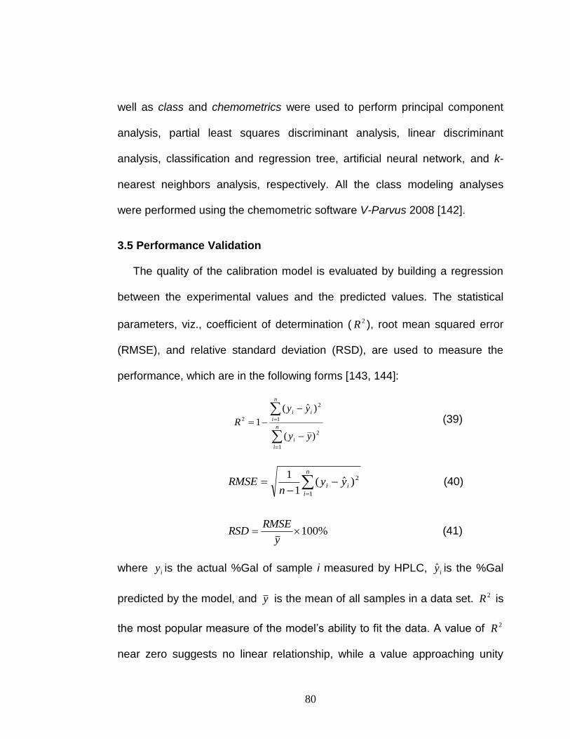
80
well as class and chemometrics were used to perform principal component
analysis, partial least squares discriminant analysis, linear discriminant
analysis, classification and regression tree, artificial neural network, and k-
nearest neighbors analysis, respectively. All the class modeling analyses
were performed using the chemometric software V-Parvus 2008 [142].
3.5 Performance Validation
The quality of the calibration model is evaluated by building a regression
between the experimental values and the predicted values. The statistical
parameters, viz., coefficient of determination ( 2R ), root mean squared error
(RMSE), and relative standard deviation (RSD), are used to measure the
performance, which are in the following forms [143, 144]:
n
i
i
n
i
ii
yy
yy
R
1
2
1
2
2
)(
)ˆ(
1 (39)
n
i
ii yyn
RMSE1
2)ˆ(1
1 (40)
%100y
RMSERSD (41)
where iy is the actual %Gal of sample i measured by HPLC, iy is the %Gal
predicted by the model, and y is the mean of all samples in a data set. 2R is
the most popular measure of the model‟s ability to fit the data. A value of 2R
near zero suggests no linear relationship, while a value approaching unity

81
indicates a near perfect linear fit. An acceptable model should have a
large 2R , a small RMSE, and a small RSD. The value of 2R will increase as
the model increases in complexity (i.e., more independent variables), so the
number of variables in the model must be considered. An alternative for 2R is
the adjusted coefficient, 2
adjR which includes the number of variables n in a
model, and favors models with a small number of variables. 2
adjR is defined by
[36]:
)1(1
11 22 R
mn
nRadj
(42)
In order to evaluate and validate the built models, training-test validation
as well as leave-one-out cross-validation (LOO-CV) methods are employed to
compare the predictive performance. For LOO-CV, the data set is divided into
n subsets: the training is performed on the (n - 1) blocks, and the test is
conducted on the objects belonging to the nth subset. In order to predict all
the objects, this process is repeated n times through block permutation [42,
103, 145].

82
Chapter IV
RESULTS AND DISCUSSION
The whole research work was divided into two parts, i.e., multivariate
regression analysis for the determination of the weight percent of
galactosamine (%Gal) and pattern recognition analysis for the differentiation
of pure, impure and contaminated heparin samples.
4.1 Multivariate Regression Analysis for Predicting %Gal
Multivariate regression (MVR) analysis of 1H NMR spectral data obtained
from heparin samples was employed to build quantitative models for the
prediction of %Gal. The MVR analysis was conducted using four separate
methods: multiple linear regression (MLR), Ridge regression (RR), partial
least squares regression (PLSR), and support vector regression (SVR).
Genetic algorithms (GAs) and stepwise selection methods were applied for
variable selection.
4.1.1 Variable Selection
In order to build robust regression models with high predictive
performance, stepwise selection methods and genetic algorithms were used
here to select a subset of variables from the original NMR spectral matrix.

83
4.1.1.1 Stepwise Procedure
In the stepwise selection, variables are added one at a time, and can be
deleted later if fail to make a significant contribution to the model. The number
of variables retained in the final model is based on the significance levels.
The Bayes information criterion (BIC) was used as a measure of the model fit,
which can be expressed as [36]:
nmnRSSnBIC log)/log( (43)
where RSS is the residual sum of squares, n is the number of samples, and
m is the number of regression variables. The variable is added to or removed
from the model in order to achieve the largest reduction of the BIC. When the
BIC value can be no longer reduced, the model selection process is stopped
resulting in the optimal subset of variables.
The variation of BIC values with the model size for all steps of the
stepwise procedure is plotted in Figure 14. Datasets A and B follow similar
trends in that each model search starts from the point in the upper left corner
of the plot, and ends in the lower right corner. The BIC measure decreases
continuously to a minimum value. However, the two datasets follow different
paths to minimize the BIC value. For Dataset A, the most highly correlated
variable, i.e., variable 2.08 ppm, entered the model first, followed by the
inclusion of variables 2.02, 2.11, 4.31, 3.53, 3.50, 5.61, and 5.34 ppm, and
then variable 2.11 ppm was dropped due to its insignificance in the model.
After that, variables 5.43, 4.25, 3.59, and 2.14 ppm were added sequentially.

84
Number of Variables
Number of Variables
Figure 14. The relationship between the Bayes information criterion (BIC) and the number of variables selected by the stepwise procedure. (A) Dataset A; (B) Dataset B.

85
Finally, the model retained 11 variables as summarized in Table 3. With
regard to Dataset B, variables 2.08, 2.02, 2.11, 1.99, 4.37, and 4.22 ppm
were added to the model step-by-step, followed by the removal of variable
2.02 ppm, the inclusion of variable 2.20 ppm, and the elimination of variable
2.11 ppm. This process led to the 5-variable subset as shown in Table 4.
Comparing the final variable subsets for Datasets A and B, the only variable
in common is 2.08 ppm. This finding implies that differences in DS content
greatly influence the selection of variables. The selected variables can be
directly used for MLR and Ridge regression analysis, or they can be
employed to derive PLSR and SVR models.
Table 3. The Stepwise Variable Selection Procedure for Dataset A
Model Size BIC Selected Variables (ppm) Add(+)/Drop(-)
1 190.97 2.08 + 2.08
2 124.81 2.02, 2.08 + 2.02
3 99.64 2.02, 2.08, 2.11 + 2.11
4 84.84 2.02, 2.08, 2.11, 4.31 + 4.31
5 76.98 2.02, 2.08, 2.11, 3.53, 4.31 + 3.53
6 56.00 2.02, 2.08, 2.11, 3.50, 3.53, 4.31 + 3.50
7 54.23 2.02, 2.08, 2.11, 3.50, 3.53, 4.31, 5.61 + 5.61
8 50.01 2.02, 2.08, 2.11, 3.50, 3.53, 4.31, 5.34, 5.61 + 5.34
7‟ 45.47 2.02, 2.08, 3.50, 3.53, 4.31, 5.34, 5.61 - 2.11
8‟ 45.05 2.02, 2.08, 3.50, 3.53, 4.31, 5.34, 5.43, 5.61 + 5.43
9 42.17 2.02, 2.08, 3.50, 3.53, 4.25, 4.31, 5.34, 5.43, 5.61 + 4.25
10 40.48 2.02, 2.08, 3.50, 3.53, 3.59, 4.25, 4.31, 5.34, 5.43, 5.61 + 3.59
11 37.49 2.02, 2.08, 2.14, 3.50, 3.53, 3.59, 4.25, 4.31, 5.34, 5.43, 5.61 + 2.14

86
Table 4. The Stepwise Variable Selection Procedure for Dataset B
Model Size BIC Selected Variables (ppm) Add(+)/Drop(-)
1 69.71 2.08 + 2.08
2 42.48 2.02, 2.08 + 2.02
3 30.73 2.02, 2.08, 2.11 + 2.11
4 27.61 1.99, 2.02, 2.08, 2.11 + 1.99
5 24.13 1.99, 2.02, 2.08, 2.11, 4.37 + 4.37
6 20.93 1.99, 2.02, 2.08, 2.11, 4.22, 4.37 + 4.22
5‟ 17.17 1.99, 2.08, 2.11, 4.22, 4.37 - 2.02
6‟ 15.50 1.99, 2.08, 2.11, 2.20, 4.22, 4.37 + 2.20
5‟‟ 14.45 1.99, 2.08, 2.20, 4.22, 4.37 - 2.11
4.1.1.2 Genetic Algorithms
As a probabilistic global optimization method in which various
combinations of variables are evaluated, GAs have been proven to be a
valuable tool for selecting optimal variables in multivariate calibration [71-77].
The approach is designed to select variables with the lowest prediction error
and is especially useful for data sets ranging between 30 and 200 variables,
and hence it is suitable for the heparin NMR datasets. GA training requires
the selection of several parameters, i.e., the number of chromosomes, initial
population, selection mode, crossover parameters, mutation rate, and
convergence criteria, all of which can influence the final results. In the present
investigation, the entire set of 74 variables was used as inputs to the GA for
selection of the subset of variables that works best for predicting %Gal.

87
Table 5. Parameters for the Genetic Algorithms
Population size 200 chromosomes
Chromosome size (the total number of variables) 74
Generation gap (initialization probability) 0.9
Crossover scheme Single-point
Crossover probability 50%
Mutation scheme Simple mutation
Mutation probability 1%
Number of generations 100
Number of variables selected in the chromosome 5, 10, 20, 30, and 40
Number of runs 500
An initial population size was set to 200, and the maximum number of
selected variables in the model was maintained between 5 and 40. The
chromosome with the maximum fitness value was chosen during each
population. The crossover probability and mutation probability were set to
50% and 1%, respectively. After a period of 100 generations, an effective
search was established. The configuration of the proposed GA is summarized
in Table 5. As the GA process is characteristically stochastic, the search
results depend on the randomly generated original population, and the
variables selected after each search process can be substantially different.
Therefore, it is necessary to carry out multiple independent runs. In this study,
each GA procedure was run 500 times, and the most frequently selected
variables were retained to build the calibration model. Figure 15 shows the
histograms of frequency with which each variable was selected in the case of
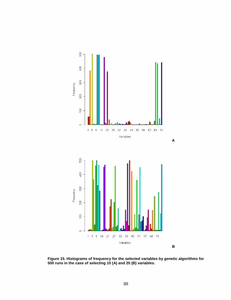
88
A
B
Figure 15. Histograms of frequency for the selected variables by genetic algorithms for 500 runs in the case of selecting 10 (A) and 20 (B) variables.

89
Table 6. The Variables (ppm) Selected by Genetic Algorithms
Number of variables Selected variables __________________________________________________________________________________
Dataset A
5 variables 2.08, 2.11, 3.50, 3.53, 4.46
10 variables 2.02, 2.08, 3.50, 3.53, 3.56, 3.71, 3.80, 5.49, 5.55, 5.67
20 variables 2.08, 2.11, 2.17, 2.20, 3.50, 3.53, 3.56, 3.71, 3.74, 3.92,
4.01, 4.04, 4.40, 4.46, 4.52, 4.92, 5.01, 5.46, 5.58, 5.67
30 variables 2.02, 2.08, 2.11, 2.14, 2.20, 3.53, 3.71, 3.74, 3.89, 3.98,
4.04, 4.13, 4.19, 4.34, 4.40, 4.46, 4.52, 4.92, 4.95, 4.98,
5.01, 5.04, 5.07, 5.22, 5.25, 5.37, 5.40, 5.58, 5.61, 5.67
40 variables 1.96, 2.02, 2.05, 2.08, 2.11, 2.14, 2.20, 3.50, 3.56, 3.59,
3.62, 3.68, 3.71, 3.74, 3.83, 3.92, 3.95, 3.98, 4.01, 4.07,
4.10, 4.31, 4.34, 4.40, 4.43, 4.49, 4.58, 4.64, 5.04, 5.07,
5.13, 5.16, 5.22, 5.31, 5.34, 5.37, 5.40, 5.46, 5.61, 5.67 Dataset B
5 variables 2.08, 3.50, 3.56, 3.71, 4.46
10 variables 2.02, 2.08, 2.14, 3.50, 3.56, 3.71, 4.46, 5.19, 5.49, 5.64
20 variables 2.02, 2.08, 2.14, 2.20, 3.50, 3.56, 3.71, 3.77, 4.07, 4.13,
4.37, 4.43, 4.46, 4.49, 4.58, 5.04, 5.10, 5.19, 5.49, 5.61
30 variables 1.96, 2.02, 2.08, 2.14, 2.20, 3.50, 3.56, 3.62, 3.71, 3.92,
3.95, 3.98, 4.07, 4.13, 4.37, 4.43, 4.46, 4.49, 4.58, 4.64,
5.04, 5.07, 5.10, 5.13, 5.16, 5.19, 5.22, 5.31, 5.49, 5.52
40 variables 1.96, 2.02, 2.05, 2.08, 2.11, 2.14, 2.20, 3.50, 3.56, 3.59,
3.62, 3.68, 3.71, 3.74, 3.83, 3.92, 3.95, 3.98, 4.01, 4.07,
4.10, 4.31, 4.34, 4.40, 4.43, 4.49, 4.58, 4.64, 5.04, 5.07,
5.13, 5.16, 5.22, 5.31, 5.34, 5.37, 5.40, 5.46, 5.61, 5.67
90
10 and 20 variables. Some variables, such as variable 5 (i.e. 2.08 ppm), are
selected each time, while others are less common. The output of the
algorithm consists of the subsets of 5, 10, 20, 30 and 40 variables which are
presented in Table 6. The most frequently selected variables are 2.08, 3.50
and 3.53 ppm, which correspond to the characteristic chemical shifts of DS.
These results added confidence that the information provided by GAs is
useful for determination of %Gal. For Dataset A, only variable 2.08 ppm was
selected in all the five subsets of variables. Other frequently selected
variables were 3.50 and 3.53 ppm. Variables 2.08, 3.50, 3.56 and 3.71 ppm
were the most frequently selected ones in Dataset B. Only two variables, 2.08
and 3.50 ppm, were found in common for both Dataset A and Dataset B.
4.1.2 Multiple Linear Regression Analysis
MLR is a simple and easy calibration method that avoids the need for
adjustable parameters such as the factor number in partial least squares
regression, the regularization parameter λ in Ridge regression, and the kernel
parameters in SVR. Consequently, MLR is among the most common
approaches used to build multivariate regression models. However, overly
complex MVR models with large numbers of independent variables may
actually lose their predictive ability. This common problem occurs when too
many variables are used to fit the calibration set, and can be solved by using
a subset of the selected variables to build the model.

91
The performance of MLR models were compared for different numbers of
variables selected by either stepwise or GA methods (Table 7). For Dataset
A, when all 74 variables were employed for the regression analysis, the
model yielded 2
adjR values of 1.000 for the training dataset but only 0.616 for
the test set. Figure 16A depicts the experimental %Gal by HPLC versus that
predicted from the NMR data. All the training sample points are located on a
straight line through the origin and with a slope equal to 1. However, many
test samples deviate from the diagonal in the plot. When MLR is trained using
all variables, some of the variables are unrelated to the variation of the
response, i.e., the %Gal. Such cases produce models that are over-fitted for
the training set but yield poor predictability for the test set.
When the most informative variables were selected, and variables that
were redundant or not correlated to the response were discarded, the
performance of the model was enhanced significantly. The predictive ability
was remarkably improved for the models up to 11 variables based on
stepwise selection. Compared to the all-variable model, the 2
adjR for the test
set increased from 0.616 to 0.976 even though the 2
adjR value for the training
set dropped slightly from 1.000 to 0.985. Taken together, these results reflect
the excellent agreement between the measured and the predicted values
after the selection of variables.

92
Table 7. Model Parameters of Multiple Linear Regression (MLR)
__________________________________________________________________________________
All Stepwise Genetic Algorithms _____ __________ ____________________________________
# of Variables 74 11 5 10 20 30 40
__________________________________________________________________________________
Model A
Dataset A
Training RMSE 0.01 0.26 0.35 0.27 0.26 0.22 0.17
RSD 0.01 0.15 0.20 0.15 0.15 0.13 0.10
2
adjR 1.000 0.985 0.971 0.983 0.985 0.989 0.993
Test RMSE 1.34 0.33 0.29 0.23 0.29 0.31 0.55
RSD 0.76 0.19 0.17 0.13 0.16 0.18 0.31
2
adjR 0.616 0.976 0.981 0.987 0.980 0.976 0.930
Dataset B
Training RMSE 0.01 0.19 0.26 0.19 0.18 0.16 0.14
RSD 0.01 0.27 0.39 0.27 0.25 0.22 0.20
2
adjR 1.000 0.860 0.784 0.861 0.892 0.901 0.918
Test RMSE 1.47 0.29 0.29 0.20 0.27 0.28 0.55
RSD 1.99 0.40 0.39 0.27 0.36 0.38 0.75
2
adjR 0.105 0.656 0.696 0.845 0.764 0.723 0.587
Model B
Dataset B
Training RMSE NA 0.21 0.18 0.13 0.10 0.07 0.03
RSD NA 0.30 0.25 0.18 0.14 0.10 0.04
2
adjR NA 0.797 0.853 0.922 0.955 0.979 0.997
Test RMSE NA 0.26 0.25 0.18 0.15 0.10 0.14
RSD NA 0.36 0.34 0.24 0.20 0.13 0.19
2
adjR NA 0.694 0.733 0.862 0.917 0.959 0.941
__________________________________________________________________________________
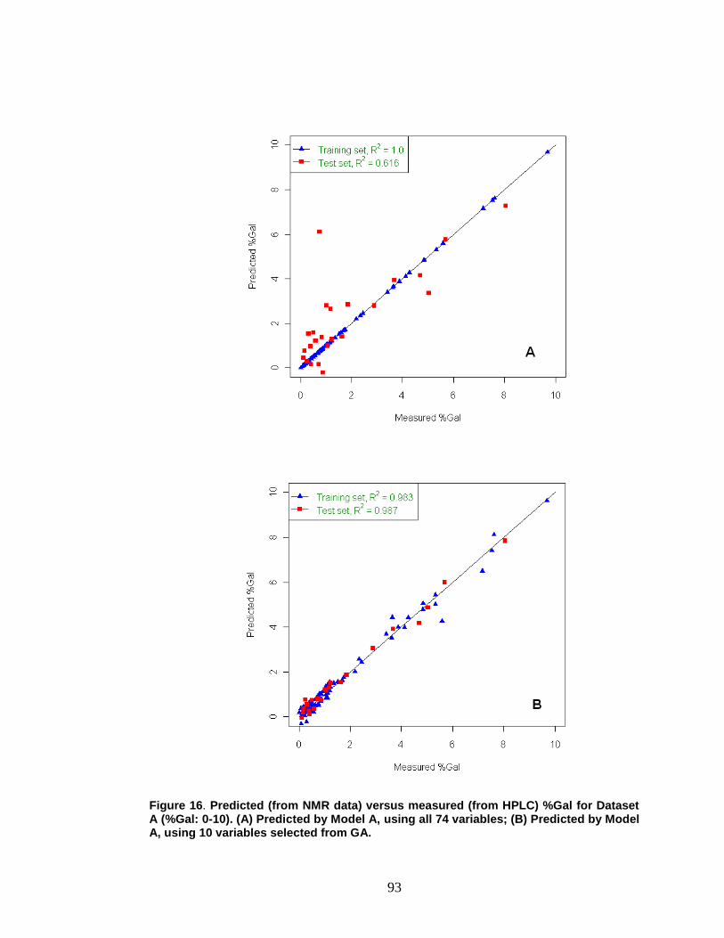
93
Figure 16. Predicted (from NMR data) versus measured (from HPLC) %Gal for Dataset A (%Gal: 0-10). (A) Predicted by Model A, using all 74 variables; (B) Predicted by Model A, using 10 variables selected from GA.

94
When considering the results from GA variable selection, the model quality
relied heavily on the number of selected variables. Table 7 shows that 2
adjR for
the training set improved continuously from 0.971 to 0.993 between 5 and 40
variables. In contrast, the test set followed a different pattern, i.e., the 2
adjR
value initially increased to a maximum 0.987 at 10 variables, after which it
gradually decreased to 0.930 at 40 variables. Therefore, the minimum
number of prediction errors occurred when the model was of moderate
complexity. In the present case, the resulting model demonstrated good
performance in estimating the %Gal concentrations at 10 variables. A strong
correlation between the measured and the predicted values over the entire
concentration range was obtained for both the training and test data sets as
illustrated in Figure 16B. Comparing the two variable selection approaches,
GA and stepwise selection, the statistical parameters 2
adjR and RMSE
revealed a slight advantage for GA over stepwise selection. The 2
adjR values
obtained using GA for variable selection were 0.981 for 5 variables and 0.980
for 20 variables, which exceed the value 0.976 for the model obtained using
stepwise variable selection.
As the USP upper limit for %Gal is 1.0%, we checked the predictive
performance of our models at low %Gal concentration. When only Dataset B
(0.0-2.0%Gal) is considered, the results predicted using Model A are only
mediocre as expected. Using the all-variable model, 2
adjR approaches 1 for the

95
training set but is unsatisfactory at 0.105 for the test set. Although variable
selection enhanced the predictive ability, the best 2
adjR for the test set was
only 0.845 at 10 variables (Figure 17A).
In order to improve the predictive ability in the lower range of 0.0-2.0%Gal,
Dataset B was employed to construct the MLR models. When building MLR
models, the number of samples must equal or exceed the number of
independent variables. The training set for Dataset B contained only 57
samples, much lower than the 74 independent variables extracted from the
NMR data, consequently the full-variable model was not feasible. The results,
summarized in Table 7, reveal that the top model performance was attained
( 2
adjR = 0.959) using a subset of 30 variables selected by GA. The superb
agreement between the predicted and experimental values (Figure 17B)
confirms the high predictive ability of Model B in the lower range of 0.0-
2.0%Gal. Stepwise variable selection yielded unsatisfactory results in terms
of the predictive ability of Model B. The 2
adjR values for the training and test
sets were 0.797 and 0.694, respectively, which were far lower than those
obtained from the corresponding GA models for any number of variables. A
possible explanation is that stepwise variable selection is limited in its ability
to explore possible combinations of variables.

96
Figure 17. Predicted (from NMR data) versus measured (from HPLC) %Gal for Dataset B (%Gal: 0-2). (A) Predicted by Model A, using 10 variables selected from GA; (B) predicted by Model B, using 30 variables selected from GA.

97
4.1.3 Ridge Regression Analysis
Multiple linear regression is very sensitive to variables with high
correlation, since near-collinearity causes a large variance or uncertainty of
the model parameters and therefore makes model predictions highly
unreliable [36]. In addition, when there are fewer samples than parameters to
be estimated, MLR method cannot be used. By applying Ridge regression
technique, the collinearity problem that happens with MLR is expected to be
solved because the X’X matrix is artificially modified so that its determinant
can be appreciably different from 0. An extra parameter is introduced in the
model, i.e., the Ridge parameter or complexity parameter λ which can
constrain the size of the regression coefficients. The value of λ determines
how much the Ridge regression deviates from the MLR regression. On one
hand, Ridge regression cannot efficiently fight collinearity if λ is too small. On
the other hand, the bias of the estimates for regression coefficients becomes
large if the value is too large.
In Ridge regression, the first step is to find the optimal parameter λ which
can produce the smallest prediction error. By estimating the prediction error
as the mean squared error for prediction (MSEP) using the generalized cross-
validation (GCV), a series of λ values corresponding to a range of variables
was obtained (Table 8). The dependence of the MSEP on the Ridge
parameter λ for the 40-variable model selected using GA is illustrated in
Figure 18A. The optimal value of λ is 0.267, which yielded the smallest

98
prediction error. The relationship between the regression coefficients and the
parameter λ is shown in Figure 18B, where the regression coefficient of each
variable is represented by a particular curve and the size changes as a
function of λ. It is clear that larger values of the Ridge parameter lead to
greater shrinkage of the coefficients which approach zero as λ approaches
infinity. The optimal choice of λ (0.267) is depicted by the vertical line in
Figure 18B, which intersects the optimized regression coefficients of the
curves.
Prediction of the test data was achieved using the optimized regression
coefficients. The statistical parameters calculated for the Ridge regression
models, including the adjusted coefficient 2
adjR , root mean squared error
(RMSE), and relative standard deviation (RSD) for both training and test sets,
are presented in Table 8. For the all-variable model, the coefficient of
determination 2
adjR for the test set increases from 0.616 to 0.801 compared
with the MLR model for Dataset A. The all-variable MLR model is unavailable
for Dataset B since the number of variables exceeds the numbers of samples.
Ridge regression is not constrained by this condition, and the all-variable
model gave 2
adjR = 1.000 for the training set and 0.778 for the test set (Table
8). The sub-optimal 2
adjR for the test set, along with the large difference
between errors for the training set and test set (0.01 to 0.38), are indicative of
model over-fitting and poor predictive ability. When the variables were

99
reduced by the stepwise and GA selection methods, the co-linearity effect
was eliminated and the predictive ability of the RR models approached that of
MLR models. Like the MLR models, the RR model showed poor predictive
ability when the model contains too few variables (under-fitting) or too many
variables (over-fitting). Therefore, selecting the appropriate number of
variables was a key factor in achieving good predictive results in Ridge
regression.
A B
Figure 18. Ridge regression for the heparin 1H NMR data at 40 variables selected from
GA. The optimal Ridge parameter λ = 0.267 is determined by generalized cross validation (GCV) (A), and the corresponding regression coefficients are the intersections of the curves of the regression coefficients with the vertical line at λ = 0.267 (B).

100
Table 8. Model Parameters of Ridge Regression (RR) __________________________________________________________________________________
All Stepwise Genetic Algorithms _____ _________ _________________________________________
# of Variables 74 11 5 10 20 30 40
__________________________________________________________________________________
Model A λ 0.01 0.28 0.18 0.56 0.64 0.34 0.27
Dataset A
Training
RMSE 0.02 0.26 0.35 0.27 0.26 0.23 0.17
RSD 0.01 0.15 0.20 0.16 0.15 0.13 0.10
2
adjR 1.000 0.985 0.971 0.983 0.984 0.987 0.992
Test
RMSE 0.93 0.32 0.28 0.23 0.29 0.33 0.64
RSD 0.53 0.18 0.16 0.13 0.17 0.19 0.36
2
adjR 0.801 0.978 0.982 0.988 0.981 0.973 0.902
Dataset B
Training
RMSE 0.02 0.18 0.27 0.18 0.17 0.15 0.14
RSD 0.03 0.26 0.38 0.26 0.24 0.22 0.20
2
adjR 0.997 0.857 0.780 0.864 0.898 0.902 0.919
Test RMSE 0.97 0.29 0.28 0.20 0.26 0.27 0.54
RSD 1.30 0.38 0.37 0.27 0.35 0.36 0.73
2
adjR 0.308 0.688 0.692 0.850 0.768 0.749 0.598
Model B λ 0.01 0.27 0.06 0.02 0.05 0.03 0.01
Dataset B
Training
RMSE 0.01 0.21 0.17 0.13 0.10 0.07 0.03
RSD 0.01 0.30 0.25 0.19 0.14 0.10 0.04
2
adjR 1.000 0.796 0.852 0.921 0.954 0.977 0.996
Test RMSE 0.23 0.26 0.25 0.18 0.15 0.11 0.14
RSD 0.31 0.35 0.34 0.24 0.20 0.14 0.19
2
adjR 0.778 0.693 0.731 0.863 0.907 0.952 0.949
__________________________________________________________________________________

101
4.1.4 Partial Least Squares Regression Analysis
As one of the most common multivariate analysis techniques, partial least
squares regression (PLSR) can be applied to spectroscopic data to transform
the large amount of correlated variables into a small set of orthogonal
variables. In PLSR, information in the independent variable matrix X is
projected onto a small number of latent variables, where the response
variable matrix Y is simultaneously used in estimating the latent variables in X
that will be most relevant for predicting the Y variables [36]. The linear
combinations of all original variables considerably reduce the dimensionality
of regression model. Unlike the MLR, variable selection is not essential for
PLSR since the latent variables are orthogonal and not sensitive to
collinearity.
The performance of PLSR depends on the selection of the appropriate
PCs used to build the regression model, and the optimal number of PCs
determines the complexity of the model and can be optimized by a leave-one-
out cross-validation (LOO-CV) procedure on the training set [76, 84]. The
optimal model size corresponds to that with the lowest uncertainty estimates
obtained from the predictive error sum of squares (PRESS). The black lines in
Figure 19 depict the standard error of prediction (SEP) values from a single
cross-validation with 10 segments while the gray lines are produced by
repeating this procedure 100 times [36]. The dashed horizontal line
represents the SEP value for the test set at the optimal number of
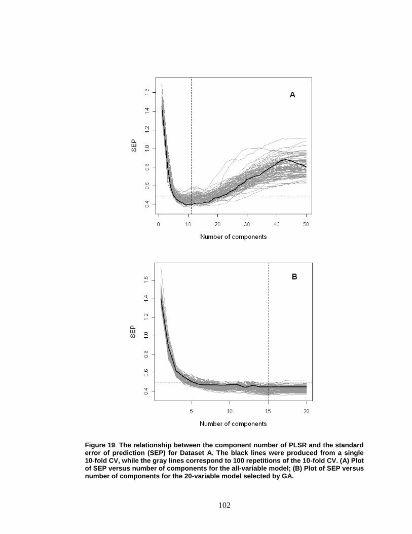
102
Figure 19. The relationship between the component number of PLSR and the standard error of prediction (SEP) for Dataset A. The black lines were produced from a single 10-fold CV, while the gray lines correspond to 100 repetitions of the 10-fold CV. (A) Plot of SEP versus number of components for the all-variable model; (B) Plot of SEP versus number of components for the 20-variable model selected by GA.

103
components depicted by the dashed vertical line. By repeating this cross-
validation procedure 100 times, the SEP variation was much larger for the all-
variable model than for the corresponding 20-variable model with variables
selected by GA indicating the latter‟s greater stability. The optimal number of
PCs was 12 and 15 corresponding to the all-variable and 20-variable models,
respectively.
Training set models were constructed using variables selected by either
GA or stepwise methods. The number of PCs previously judged to be optimal
was employed and the computed models were applied to the test set. The
optimal number of PCs for each model, along with corresponding values
of 2
adjR , RMSE, and relative standard error (RSE), are summarized in Table 9.
As mentioned above, the all-variable model required 12 PCs which
corresponded to the minimal cross-validation error. PLSR models built using
11 variables selected by the stepwise method yielded 2
adjR = 0.984 for the
training set and 0.979 for the test set. The prediction performance of the
model for %Gal was also satisfactory using GA for variable selection. The
prediction performance of the model with 5 to 20 variables selected by GA
was better than the all-variable model. The 10-variable model, which gave a
high 2
adjR of 0.988 and a low RSD of 0.124 (Table 9), was therefore chosen as
the optimal model.

104
Table 9. Model Parameters of Partial Least Squares Regression (PLSR)
__________________________________________________________________________________
All Stepwise Genetic Algorithms _____ ___________ __________________________________
# of Variables 74 11 5 10 20 30 40 __________________________________________________________________________________
Model A
Optimal PCs 12 8 5 8 15 18 22
Dataset A
Training RMSE 0.16 0.26 0.35 0.27 0.26 0.26 0.23
RSD 0.09 0.15 0.20 0.16 0.15 0.15 0.13
2
adjR 0.994 0.984 0.972 0.982 0.983 0.985 0.988
Test RMSE 0.39 0.31 0.29 0.22 0.28 0.33 0.37
RSD 0.22 0.18 0.17 0.12 0.16 0.19 0.21
2
adjR 0.962 0.979 0.980 0.989 0.982 0.974 0.970
Dataset B
Training RMSE 0.14 0.17 0.26 0.23 0.19 0.18 0.16
RSD 0.20 0.25 0.38 0.33 0.27 0.25 0.24
2
adjR 0.912 0.869 0.784 0.817 0.863 0.868 0.897
Test RMSE 0.29 0.27 0.29 0.20 0.26 0.27 0.28
RSD 0.39 0.36 0.39 0.26 0.35 0.36 0.38
2
adjR 0.696 0.740 0.694 0.855 0.751 0.735 0.718
Model B Optimal PCs 28 5 5 9 19 23 34
Dataset B
Training RMSE 0.03 0.20 0.17 0.13 0.10 0.06 0.04
RSD 0.04 0.28 0.25 0.18 0.13 0.09 0.05
2
adjR 0.994 0.799 0.855 0.924 0.958 0.980 0.987
Test RMSE 0.20 0.26 0.25 0.18 0.15 0.09 0.14
RSD 0.27 0.34 0.33 0.24 0.20 0.12 0.19
2
adjR 0.846 0.697 0.733 0.864 0.917 0.965 0.948
__________________________________________________________________________________

105
When the %Gal of Dataset B (%Gal = 0.0-2.0) was predicted by Model B,
the all-variable PLSR model yielded 2
adjR = 0.846 and RMSE = 0.20 (Table 9).
Variable selection by GAs on the Dataset B greatly enhanced the prediction
performance. The optimal model occurred using 30 variables with an 2
adjR
value of 0.965 for the test set.
4.1.5 Support Vector Regression Analysis
In multivariate regression models (i.e. MLR and PLSR), a linear
relationship is assumed between the NMR spectral variables and the %Gal.
Consequently, the predictive ability of a model will suffer if the actual
relationship between the dependent and independent variables is non-linear
rather than linear. In these cases, regression methods that encompass both
linear and non-linear models represent an effective strategy. Support vector
regression (SVR) processes both linear and non-linear relationships by using
an appropriate kernel function that maps the input matrix X onto a higher-
dimensional feature space and transforms the non-linear relationships into
linear forms [82, 83]. This new feature space is then implemented to deal with
the regression problem [85]. We employed SVR to construct both linear and
nonlinear prediction models for assessing whether nonlinear regression
models would improve prediction results on the same datasets.
Therefore, initially the proper kernel functions were selected and then
optimized for a specific parameter. Unlike the Lagrange multipliers which can

106
be optimized automatically by the program, SVR requires the user to adjust
the kernel parameters, the radius of the tube ε, and the regularizing
parameter C. When applying the RBF kernel, the generalization property is
dependent on the parameter γ which controls the amplitude of the kernel
function. If γ is too large, all training objects are used as the support vectors
leading to over-fitting. If γ is too small, all data points are regarded as one
object resulting in poor ability to generalize [83]. In addition, the penalty
weight C and the tube size ε also require optimization. As the regularization
parameter, C controls the trade-off between minimizing the training error and
maximizing the margin. Generally, values of C that are too large or too small
lead to regression models with poor prediction ability. When C is very low, the
predictive ability of the model is exclusively determined by the weights of
regression coefficients [86]. When C is large, the cost function decides the
performance while the regression coefficients have little bearing even if their
values are very high. Data points with prediction errors larger than ±ε are the
support vectors which determine the predictive ability of the SVR model. A
large number of support vectors occur at low ε, while sparse models are
obtained when the value of ε is high. The optimal value of ε depends heavily
on the individual datasets. Small values of ε should be used for low levels of
noise, whereas higher values of ε are appropriate for large experimental
errors. Thus, in order to find the optimized combination of the parameters γ, C
and ε, cross validation via parallel grid search was performed.

107
Table 10. Model Parameters for Support Vector Regression with RBF Kernel
__________________________________________________________________________________
All Stepwise Genetic Algorithms _____ ___________ __________________________________
# of Variables 74 11 5 10 20 30 40 __________________________________________________________________________________
Model A
SVR parameters ε 0.14 0.01 0.18 0.10 0.07 0.05 0.10
C × 10-4
10 1.0 10 100 10 10 1.0
Γ × 105 1.0 1.0 1.0 1.0 1.0 1.0 1.0
# of Vectors 28 71 21 43 39 59 37 Dataset A
Training RMSE 0.22 0.28 0.36 0.28 0.27 0.25 0.24
RSD 0.13 0.16 0.21 0.16 0.16 0.14 0.14
2
adjR 0.989 0.983 0.971 0.983 0.984 0.986 0.987
Test RMSE 0.43 0.25 0.28 0.23 0.22 0.21 0.41 RSD 0.243 0.14 0.16 0.13 0.13 0.12 0.23
2
adjR 0.956 0.985 0.983 0.987 0.988 0.990 0.960
Dataset B
Training RMSE 0.21 0.18 0.27 0.17 0.17 0.16 0.15
RSD 0.31 0.25 0.39 0.25 0.24 0.23 0.22
2
adjR 0.816 0.863 0.774 0.878 0.884 0.896 0.901
Test RMSE 0.39 0.23 0.25 0.20 0.18 0.16 0.36
RSD 0.53 0.31 0.34 0.26 0.24 0.22 0.49
2
adjR 0.663 0.783 0.761 0.839 0.870 0.887 0.701
Model B
SVR parameters ε 0 0.60 0.15 0.40 0.03 0.05 0.07
C × 10-5
10 10 1.0 10 10 10 10
Γ × 105 1.0 1.0 100 1.0 1.0 1.0 1.0
# of Vectors 57 16 39 15 53 51 49 Dataset B
Training RMSE 0.02 0.21 0.14 0.14 0.10 0.07 0.04
RSD 0.02 0.30 0.21 0.19 0.14 0.10 0.05
2
adjR 0.999 0.787 0.902 0.913 0.958 0.976 0.994
Test RMSE 0.20 0.24 0.23 0.18 0.16 0.10 0.15
RSD 0.27 0.33 0.32 0.24 0.21 0.13 0.20
2
adjR 0.821 0.736 0.756 0.868 0.913 0.960 0.922
__________________________________________________________________________________

108
The values of the optimal parameters γ, C and ε as well as the predicted
results of the optimal SVR models are shown in Table 10. For Dataset A, the
coefficient of determination 2
adjR between the measured and predicted %Gal
for the test set was 0.956 for the all-variable model yielded. The predictive
ability of the model with variables selected by GA gradually increased starting
with 5 variables, reached a maximum at 30 variables, and then receded
beyond this number. The 2
adjR values for the test set were 0.983, 0.987, 0.988,
0.990, and 0.960 corresponding to 5, 10, 20, 30, and 40 variables.
As with RR and PLSR, SVR model performance was poorer for Dataset B
than for Dataset A. For the all-variable models, the RBF kernel yielded 2
adjR =
0.999 for the training set, but only 0.821 for the test set, suggesting the
existence of over-fitting. The predictive ability of the models improved
considerably using GA for variable selection with an appropriate number of
variables. A maximum 2
adjR of 0.960 for the test set was achieved at 30
variables.
4.2 Classification of Pure and Contaminated Heparin Samples
Preliminary screening of contaminated heparin batches collected from
different sources by means of 1H NMR spectroscopy and capillary
electrophoresis (CE) revealed four different groups, i.e., pure heparin with
almost no DS, heparin containing DS in varying amounts but without OSCS,

109
heparin with OSCS and without DS, and heparin with both OSCS and DS. In
this study, 178 heparin samples from various suppliers were analyzed, where
the DS content is up to 19% of the polymer mixture and the OSCS varies
from 0 to 27%. The new USP specification states that the impurity acceptance
limit for DS is 1.0%, and no any OSCS level is acceptable. Thus, the 178
samples were classified into three groups, i.e., pure heparin with DS ≤ 1%
and OSCS = 0%; impure heparin with DS > 1% and OSCS = 0%; and
contaminated heparin with OSCS > 0% and any content of DS.
The high-resolution 1H NMR spectroscopy data were represented as
complex matrices with rows as objects and columns as variables. By applying
multivariate statistical methods and pattern recognition techniques, the
dimensionality of the data can be reduced to facilitate visualization, the
inherent patterns among the sets of spectral measurements can be revealed,
and classification models can be built. As one of the fundamental
methodologies in chemometrics, the purpose of classification is to find a
mathematical model to recognize the class membership of new objects by
assigning a proper class. In this study, the NMR data were analyzed by both
the unsupervised approaches such as principal component analysis (PCA)
and the supervised ones such as partial least squares discriminant analysis
(PLS-DA) to distinguish the pure and contaminated heparin samples.

110
4.2.1 Principal Components Analysis
Principal components analysis (PCA) is a nonparametric approach that
reduces a complex dataset to lower dimensions, performs the optimum
coordinate rotation, and maximize the variance within the data [36, 40]. In this
study, PCA is employed to provide an overview of the spectral data, from
which a general picture of the classification of heparin samples into groups
can be acquired. Since PCA preserves most of the variance in just a few
numbers of principal components (PCs), this information can be readily
displayed in a graph of reduced dimensions and data can be visualized by
using the scores plots that differentiate samples from various sources based
on the measured properties. The most common way is to project the spectra
into the subspace of PC1 versus PC2 with PC1 along the x-axis and PC2
along the y-axis, where the sample distribution on this graph may reveal
patterns, clusters and other features that might be related to the general
characteristics of the samples [44-46].
The PCA scores plots obtained from analysis of the 1H NMR spectra for
representative heparin samples are shown in Figures 20A, 21A and 22A.
Each point on the plots represents one spectrum of an individual sample, and
points of the same color indicate samples of the same origin, such as pure
heparin, heparin with the impurity DS, or heparin with the contaminant OSCS.
The spectra with similar characteristics form a cluster and the variations along
the PC axes maximize the differences between the spectra. The Heparin and
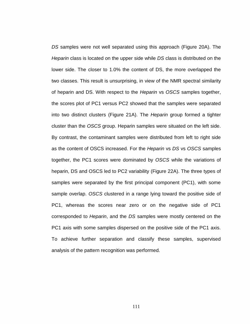
111
DS samples were not well separated using this approach (Figure 20A). The
Heparin class is located on the upper side while DS class is distributed on the
lower side. The closer to 1.0% the content of DS, the more overlapped the
two classes. This result is unsurprising, in view of the NMR spectral similarity
of heparin and DS. With respect to the Heparin vs OSCS samples together,
the scores plot of PC1 versus PC2 showed that the samples were separated
into two distinct clusters (Figure 21A). The Heparin group formed a tighter
cluster than the OSCS group. Heparin samples were situated on the left side.
By contrast, the contaminant samples were distributed from left to right side
as the content of OSCS increased. For the Heparin vs DS vs OSCS samples
together, the PC1 scores were dominated by OSCS while the variations of
heparin, DS and OSCS led to PC2 variability (Figure 22A). The three types of
samples were separated by the first principal component (PC1), with some
sample overlap. OSCS clustered in a range lying toward the positive side of
PC1, whereas the scores near zero or on the negative side of PC1
corresponded to Heparin, and the DS samples were mostly centered on the
PC1 axis with some samples dispersed on the positive side of the PC1 axis.
To achieve further separation and classify these samples, supervised
analysis of the pattern recognition was performed.

112
Figure 20. Scores plots for the model Heparin vs DS. (A) PCA; (B) PLS-DA.

113
Figure 21. Scores plots for the model Heparin vs OSCS. (A) PCA; (B) PLS-DA.

114
Figure 22. Scores plots for the model Heparin vs DS vs OSCS. (A) PCA; (B) PLS-DA.

115
4.2.2 Partial Least Squares Discriminant Analysis
To optimize separation between heparin and impure or contaminated
samples and to build predictive models for class identification, PLS-DA was
performed using the classes of Heparin, DS or OSCS as the y variables. The
scores plots of the first and the second latent variables are displayed in
Figures 20B, 21B and 22B. With PLS-DA, nearly all samples were in distinct
classes, and a clear discrimination of heparin samples from the DS impurity
and OSCS contaminant was observed. Here, the heparin samples appeared
in a more compact grouping, while the OSCS contaminated samples
exhibited a distribution similar to that in the PCA model. Applying PLS-DA, the
correct classification of these samples in three different groups was obtained
as shown in Figure 22B, where Heparin and DS were located in the upper-
and lower-left zones, respectively, while OSCS was distributed toward the
right side. This supervised clustering approach gave much improved
separation compared with the PCA model, and excellent class discrimination
was achieved between the different types of heparin samples.
After PLS data compression, PLS-DA classification models were built and
tested while increasing the number of PLS components starting at 1. The
number of correct classifications in both the training and test sets was taken
as a measure of performance. Figure 23 illustrates the evolution of the
misclassification rates in the training and test sets as a function of the number
of PLS components in the model. As expected for the training set, the number

116
of correct classifications increased with the number of dimensions (PCs). For
any model, the misclassification rates were small even with few PLS
components and reached a plateau at which all the rates approached zero
after 20 to 40 components.
A B
C D
Figure 23. Misclassification rate as a function of the number of PLS dimensions for the PLS-DA model. (A) Heparin vs DS; (B) Heparin vs OSCS; (C) Heparin vs [DS + OSCS]; (D) Heparin vs DS vs OSCS.

117
Leave-one-out cross-validation (LOO-CV) was employed to select the
model with the optimal number of PLS components that minimize the
misclassification rate. For LOO-CV, the data set was split into s segments:
the training was performed on the (s - 1) blocks, and the testing was
conducted on the objects belonging to the sth subset. To predict all the
objects, this process was repeated s times through block permutation [104,
145]. Classification rates of 85, 97 and 82% were obtained for Heparin vs DS,
Heparin vs OSCS, and Heparin vs [DS + OSCS] models, respectively. In
addition, a 75% classification rate was attained by the threefold Heparin vs
DS vs OSCS model. The majority of misclassifications between Heparin and
DS involved cases where the DS content was close to the 1.0% DS boundary
between the two classes, as measured by HPLC measurements.
The true test of the model depends on its performance when applied to an
external test set of samples that were not employed for building the model.
Consequently, the model was validated using an external test set of 60
samples. The results, plotted in Figure 23, point to the same conclusions as
described above for the LOO-CV. By increasing the number of PLS
components incrementally, it was observed that the classification rates were
optimal for the Heparin vs DS (84%), Heparin vs OSCS (100%), and Heparin
vs [DS + OSCS] (88%) models when the number of PCs = 2-6, 10-12, and 6-
10, respectively. Even for the threefold Heparin vs DS vs OSCS model, the
classification rate was 85% using 16 PCs.

118
Table 11. Number and Type of Misclassifications (Errors) by PLS-DA Classification
Model for Test Sets Using Different Number of Components
Components 1 2 4 6 8 10 12 14 16 18 20 __________________________________________________________________________________
Model
Heparin vs DS
Heparin errors / 28 samples 4 2 1 1 2 4 4 5 5 5 6
DS errors / 17 samples 5 5 6 6 6 6 7 7 7 8 8
Heparin vs OSCS
Heparin errors / 28 samples 0 0 0 0 0 0 0 1 1 1 1
OSCS errors / 15 samples 3 2 2 1 1 0 0 0 1 1 1
Heparin vs [DS + OSCS]
Heparin errors / 28 samples 3 4 2 1 2 2 3 3 4 5 8
[DS + OSCS] errors / 32 samples 9 6 7 6 5 5 5 5 5 6 8
Heparin vs DS vs OSCS
Heparin errors / 28 samples 4 3 1 1 1 2 3 3 3 3 4
DS errors / 17 samples 7 7 7 8 8 8 7 7 5 7 8
OSCS errors / 15 samples 6 6 5 4 2 1 1 1 1 1 2
The results for the corresponding test sets are presented in Table 11. For
the Heparin vs DS model using 4-6 PCs, misclassification of Heparin as DS
occurred only once and DS as Heparin six times. In nearly all of these cases
the DS content was 1.06-1.20%, i.e., near the 1.0% boundary specifying the
two classes. For the Heparin vs OSCS model using 1-12 PCs,
misclassification of Heparin as OSCS was zero (100% success rate) and
OSCS for Heparin varied from 0 to 3. The number of misclassifications was
zero (100% success rate) for the Heparin vs OSCS model using 10-12 PCs.

119
For the Heparin vs [DS + OSCS] model using 8-10 PCs, only two Heparin
samples and five samples in the [DS + OSCS] group were misclassified. As
noted for the Heparin vs DS model, in most cases these misclassifications
occurred when the DS content was near the 1.0% DS boundary defining the
Heparin and DS classes. The same interpretation applies to the threefold
Heparin vs DS vs OSCS model, where most of the misclassifications involved
samples near the 1.0% DS borderline between Heparin and DS. Notably, the
discrimination between the Heparin and OSCS samples was 100%.
4.2.3 Linear Discriminant Analysis
As an alternative approach, linear discriminant analysis (LDA) was
employed to classify the Heparin, DS and OSCS samples based on
predefined classes. For LDA analysis, the data matrix of variances-
covariances needs to be inverted, which would be impossible if the number of
samples is less than that of the variables [79, 93]. Therefore, a preliminary
variable reduction step is necessary so that the data matrix for each class
presents a high ratio between the number of training samples and the number
of variables. In order to select a subset of the original variables that affords
the maximum improvement of the discriminating ability between classes,
stepwise linear discriminant analysis (SLDA) was performed before LDA
analysis. Preliminary variable reduction using SLDA led to the selection of 20
variables (Table 12).

120
Table 12. Wilks’ Lambda ( v ) & F-to-enter (F) of Variables (V) for Various Models
__________________________________________________________________________________
Order Heparin vs DS Heparin vs OSCS Heparin vs [DS + OSCS] Hearin vs DS vs OSCS
V (ppm) v F V (ppm) v F V (ppm) v F V (ppm) v F
__________________________________________________________________________________
1 2.08 103.0 0.54 2.14 14.0 0.36 2.08 97.1 0.63 2.11 134.3 0.38
2 3.62 15.8 0.48 2.08 15.1 0.33 4.49 23.3 0.55 3.86 30.9 0.28
3 5.34 8.9 0.45 4.49 8.1 0.29 2.14 3.6 0.52 3.53 9.2 0.25
4 2.17 1.7 0.44 4.16 6.7 0.26 4.16 5.3 0.50 4.49 7.1 0.23
5 2.14 2.3 0.43 4.04 5.5 0.24 4.46 3.3 0.49 5.16 10.1 0.20
6 4.61 1.5 0.42 3.56 2.5 0.22 5.16 2.7 0.47 3.59 6.5 0.19
7 2.11 1.1 0.42 4.52 5.2 0.21 5.10 2.6 0.46 2.14 4.1 0.18
8 3.95 2.1 0.41 3.65 4.2 0.20 5.61 2.8 0.46 3.95 4.4 0.17
9 5.67 1.2 0.41 5.61 8.0 0.19 4.28 3.9 0.45 4.46 3.5 0.16
10 4.04 1.9 0.40 5.67 4.0 0.18 3.56 4.1 0.44 5.01 3.5 0.15
11 5.43 1.6 0.40 4.37 1.9 0.18 4.95 2.2 0.43 4.43 3.0 0.15
12 3.71 1.1 0.39 5.25 4.4 0.17 5.49 3.8 0.42 3.71 5.3 0.14
13 4.46 1.7 0.39 3.74 3.1 0.16 4.98 1.9 0.41 5.13 2.1 0.14
14 3.77 1.7 0.39 5.04 3.9 0.15 4.61 2.2 0.40 5.04 2.5 0.13
15 3.74 1.5 0.38 2.17 2.4 0.15 4.22 1.0 0.40 5.46 1.5 0.13
16 5.40 1.7 0.38 5.49 3.5 0.14 5.19 2.2 0.40 4.64 2.1 0.13
17 3.68 1.0 0.37 3.68 2.7 0.14 5.43 1.9 0.39 4.13 1.8 0.12
18 4.01 1.1 0.37 4.10 3.9 0.13 4.34 1.1 0.39 4.16 1.5 0.12
19 5.19 1.6 0.37 5.28 4.0 0.13 5.58 1.4 0.39 4.28 1.9 0.12
20 5.31 1.5 0.36 5.19 2.3 0.12 5.25 1.6 0.38 4.22 1.8 0.11 __________________________________________________________________________________
After variable selection and dimension reduction, LDA analysis was
conducted using the squared Mahalanobis distance from the centers of
gravity of each group for assigning the class affiliation of each sample. For
the training set, the success rates gradually rose with increasing the number
of variables (Table 13). The Heparin vs OSCS model required very few
variables to achieve 100% success rates due to the clear distinction in

121
Table 13. Performance of LDA Classification Models under Different Variables
Number of variables 2 4 6 8 10 12 14 16 18 20
Model
Heparin vs DS
Training set Errors / 87 samples 14 12 10 10 9 9 8 6 5 3
Success rates (%) 84 86 89 89 90 90 91 93 94 97
CV set Errors / 87 samples 15 13 12 12 10 10 12 13 14 14
Success rates (%) 83 85 86 86 89 89 86 85 84 84
Test set Errors / 45 samples 7 6 5 5 6 6 7 8 8 10
Success rates (%) 84 87 89 89 87 87 84 82 82 78
Heparin vs OSCS
Training set Errors / 85 samples 6 4 4 2 1 1 0 0 0 0
Success rates (%) 93 95 95 98 99 99 100 100 100 100
CV set Errors / 85 samples 6 5 4 4 2 0 1 2 3 5
Success rates (%) 93 94 95 95 98 100 99 98 97 94
Test set Errors / 43 samples 2 1 1 1 0 0 1 2 2 3
Success rates (%) 95 98 98 98 100 100 98 95 95 93
Heparin vs [DS + OSCS]
Training set Errors / 118 samples 17 15 14 14 13 13 12 10 9 9
Success rates (%) 86 87 88 88 89 89 90 92 93 93
CV set Errors / 118 samples 19 18 18 16 14 11 10 12 15 17
Success rates (%) 84 85 85 86 88 91 92 90 87 86
Test set Errors / 60 samples 7 6 5 5 4 5 6 6 6 8
Success rates (%) 88 90 92 92 93 92 90 90 90 87
Heparin vs DS vs OSCS
Training set Errors / 118 samples 26 24 21 19 16 14 12 12 10 8
Success rates (%) 78 80 82 84 86 88 90 90 92 93
CV set Errors / 118 samples 28 27 25 19 15 13 16 18 19 21
Success rates (%) 76 77 79 84 87 89 86 85 84 82
Test set Errors / 60 samples 12 11 10 9 6 6 8 8 10 10
Success rates 80 82 83 85 90 90 87 87 83 83

122
spectral features between heparin and OSCS. Cross validation and external
validation studies indicated that model performance reached a maximum
using an intermediate number of variables. LDA models typically include a set
of tunable parameters, the number of which increases with the number of
variables. While even models with complex relationships in the sample can
usually be fit quite well by using enough tunable parameters, this typically
leads to much higher error rates for the test set than for the training set as
occurred in the present instance.
The risks of over-fitting can be alleviated by selecting the optimal number
of variables, which was determined by the success rate of classifications
using LOO-CV and validation with external test sets. Optimal success rates,
varying from 89% to 100%, for the Heparin vs DS, Heparin vs OSCS, Heparin
vs [DS + OSCS] models were achieved using 6-14 variables depending on
the specific model and testing procedure (Table 13). In the same way, the
threefold Heparin vs DS vs OSCS model achieved an optimal success rate of
89% using 10-12 variables. Once again, the majority of misclassifications are
attributed to Heparin and DS samples in which the DS content was near the
1.0% boundary between the two classes.
With respect to classification of individual samples and overall success
rates, the performance of LDA was comparable to PLS-DA for the Heparin vs
OSCS model and superior to PLS-DA for other three models. For the external
test set under optimal conditions, the success rates for the Heparin vs DS,

123
Heparin vs [DS + OSCS], and Heparin vs DS vs OSCS models were
respectively 89, 93, and 90% using LDA compared to 84, 88 and 85% using
PLS-DA.
4.2.4 k-Nearest-Neighbor
The kNN method was implemented to evaluate its performance for
classification. Various k values (3, 5 or 7) were tested using the all-variable
data set, and the success rates for the training set, LOO-CV, and the test set
are summarized in Table 14. Overall, the results obtained were inferior for
kNN compared with LDA and PLS-DA. For example, the success rates for the
Heparin vs DS, Heparin vs OSCS, Heparin vs [DS + OSCS], and Heparin vs
DS vs OSCS models using k = 3 were respectively 69, 91, 82 and 68% for the
test set.
To obtain better classification results, the PCA scores were employed as
inputs to build the kNN models. Various combinations of PCs and k values
were investigated, and the results are summarized in Table 15. Unlike the
PLS-DA and LDA models where the misclassification rates for the training set
decreased monotonically to 0% as the number of PCs or variables increased,
the misclassification rates of the kNN models for the training set fluctuated
within a range of values. This fluctuating pattern is commonly observed with
kNN. The optimal performance of the kNN model was achieved using 15-25
PCs depending on the specific model.

124
Table 14. Performance of kNN Classification Models for Original Data
Model Hep vs DS Hep vs OSCS Hep vs [DS + OSCS] Hep vs DS vs OSCS
k = 3 Training set
Errors / samples 7 / 87 1 / 85 13 / 118 16 / 118
Success rate (%) 92 99 89 86
LOO-CV set
Errors / samples 16 / 87 4 / 85 25 / 118 32 / 118
Success rate (%) 82 95 79 73
Test set
Errors / samples 14 / 45 4 / 43 11 / 60 19 / 60
Success rate (%) 69 91 82 68
k = 5 Training set
Errors / samples 12 / 87 2 / 85 17 / 118 21 / 118
Success rate (%) 86 98 86 82
LOO-CV set
Errors / samples 17 / 87 5 / 85 25 / 118 30 / 118
Success rate (%) 81 94 79 75
Test set
Errors / samples 13 / 45 4 / 43 11 / 60 22 / 60
Success rate (%) 71 91 82 63
k = 7 Training set
Errors / samples 13 / 87 2 / 85 17 / 118 20 / 118
Success rate (%) 85 98 86 83
LOO-CV set
Errors / samples 14 / 87 5 / 85 27 / 118 33 / 118
Success rate (%) 84 94 77 72
Test set
Errors / samples 13 / 45 4 / 43 13 / 60 21 / 60
Success rate (%) 71 91 78 65

125
Table 15. Performance of PCA-kNN Classification Models under Different PCs
PCs 5 10 15 20 25 30 35 40 45 50 55 60
Heparin vs DS (k = 2)
Training set Errors / 87 samples 13 11 7 5 12 8 10 12 10 13 15 14
Success rates (%) 85 87 92 94 86 91 89 86 89 85 83 84
CV set Errors / 87 samples 25 20 17 20 25 25 27 22 29 34 31 33
Success rates (%) 71 77 80 77 71 71 69 75 67 61 64 62
Test set Errors / 45 samples 12 15 16 12 10 14 12 15 15 12 16 19
Success rates (%) 73 67 64 73 78 69 73 67 67 73 64 58
Heparin vs OSCS (k = 4)
Training set Errors / 85 samples 6 3 5 5 9 8 8 11 11 16 13 19
Success rates (%) 93 96 94 94 89 91 91 87 87 81 85 78
CV set Errors / 85 samples 10 13 11 10 14 18 19 25 22 24 25 26
Success rates (%) 88 85 87 88 84 79 78 71 74 72 71 69
Test set Errors / 43 samples 37 38 40 39 39 37 30 33 33 31 30 33
Success rates (%) 86 88 93 91 91 86 70 77 77 72 70 77
Heparin vs [DS + OSCS] (k = 3)
Training set Errors / 118 samples 17 10 13 17 19 11 16 14 18 17 19 25
Success rates (%) 86 92 89 86 84 91 86 88 85 86 84 79
CV set Errors / 118 samples 23 30 26 34 33 39 31 28 34 36 34 43
Success rates (%) 81 75 78 71 72 67 74 76 71 69 71 64
Test set Errors / 60 samples 13 13 12 9 17 15 17 19 23 22 22 21
Success rates (%) 78 78 80 85 72 75 72 68 62 63 63 65
Heparin vs DS vs OSCS (k = 3)
Training set Errors / 118 samples 18 13 19 23 22 17 21 21 23 23 25 32
Success rates (%) 85 89 84 81 81 86 82 82 81 81 78 73
CV set Errors / 118 samples 30 39 32 42 42 40 43 43 47 41 46 52
Success rates (%) 75 67 73 64 64 66 64 64 60 65 61 56
Test set Errors / 60 samples 21 19 18 15 20 23 23 23 25 24 27 27
Success rates 65 68 70 75 67 62 62 62 58 60 55 55

126
The misclassification rates for nearest neighbors k from 1 to 25 are plotted
in Figure 24. The black dots and the vertical bars represent the means as well
as mean ±1 standard error for the misclassification rates using LOO-CV. The
smallest LOO-CV error is depicted by a dotted horizontal line corresponding
to the position of the mean plus one standard error. For the training sets, the
misclassification rate was always zero for k = 1 and increased with larger k
values for all four models. The test sets showed a similar pattern, i.e., the
misclassification rates varied within a tight range, except the Heparin vs
OSCS model for which the rates rose for k > 4. The optimal k values of 2, 4, 3
and 3 respectively were for the Heparin vs DS, Heparin vs OSCS, Heparin vs
[DS + OSCS], and Heparin vs DS vs OSCS models.
When the predictive ability was evaluated for the external test set based
on the above analysis for different numbers of PCs and a series of k values,
the optimal success rates were 78, 93, 83 and 75% for the four models as
shown in Table 15. For the Heparin vs DS model, one heparin sample was
misclassified as DS but nine out of the seventeen DS test samples were
misclassified as Heparin. Unlike PLS-DA and LDA, kNN was unable to
completely discriminate Heparin and OSCS. For the Heparin vs [DS + OSCS]
model, three Heparin samples were misclassified as [DS + OSCS] while six
DS samples and one OSCS sample were misclassified as Heparin. Likewise
for the threefold Heparin vs DS vs OSCS model, kNN produced a total of
fifteen misclassifications.
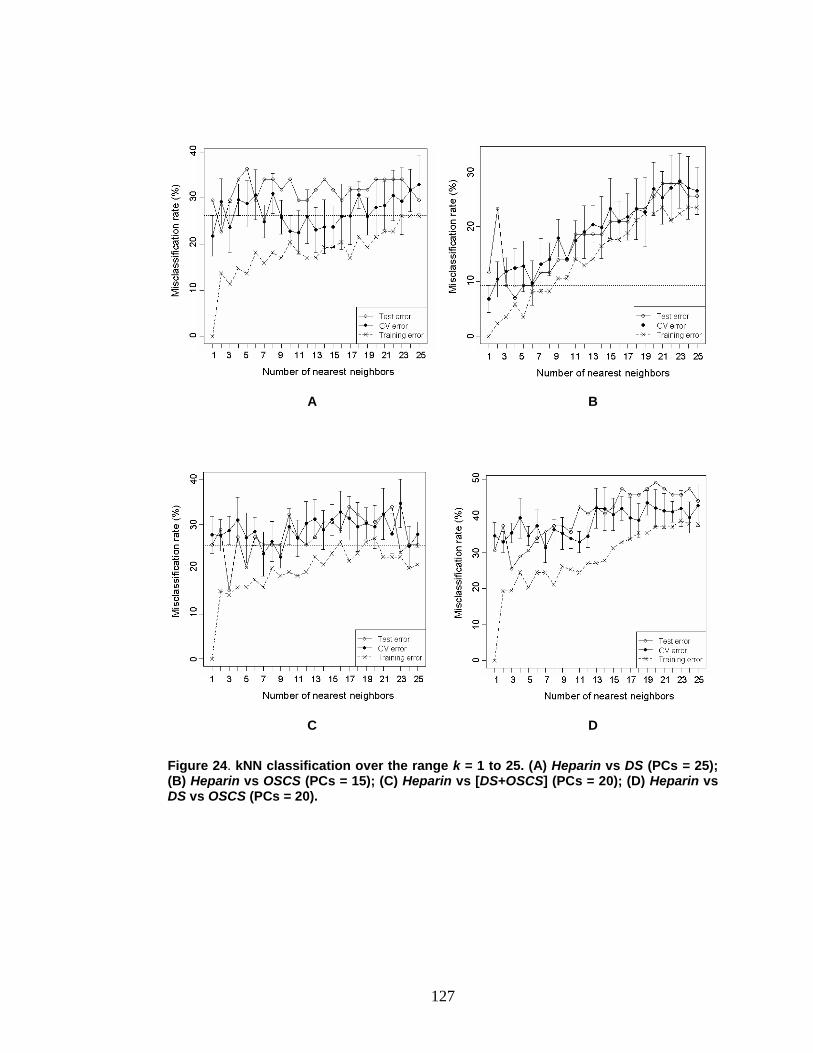
127
A B
C D
Figure 24. kNN classification over the range k = 1 to 25. (A) Heparin vs DS (PCs = 25); (B) Heparin vs OSCS (PCs = 15); (C) Heparin vs [DS+OSCS] (PCs = 20); (D) Heparin vs DS vs OSCS (PCs = 20).

128
4.2.5 Classification and Regression Tree
Classification tree models were built using the three data sets, composed
of 9, 65 and 74 variables corresponding to the three regions 1.95-2.20, 3.10-
5.70 and 1.95-5.70 ppm, respectively. The four known classes (Heparin, DS,
OSCS and [DS + OSCS]) were used as response variables. The trees were
grown and pruned using the Gini index as a splitting criterion and the optimal
size of the tree was determined using 10-fold cross validation (CV), in which
the samples are randomly divided into 10 segments, and then a model is built
on nine segments and the remaining one is used for evaluating the predictive
power until each segment has been used once as a test set. For Heparin vs
DS vs OSCS in the region of 1.95-2.20 ppm, the division of the samples by
the nodes of the classification tree is shown in Figure 25A. The data were
split according to 2.08 and 2.15 ppm, the characteristic chemical shifts of DS
and OSCS, respectively. It is observed that the first split is defined by variable
2.15 ppm that split the samples into two groups: (Heparin + DS) and OSCS,
and then variable 2.08 ppm divided the (Heparin + DS) samples into two
separate classes: Heparin and DS, leading to a classification tree with a
complexity of three nodes (Figure 25C).
Each terminal node represents the majority of the samples in a specified
class. The OSCS terminal node is called a pure node in that it contains only
samples of the OSCS class, i.e., all of the 31 OSCS samples are correctly
classified and no Heparin or DS samples are located in this terminal. The
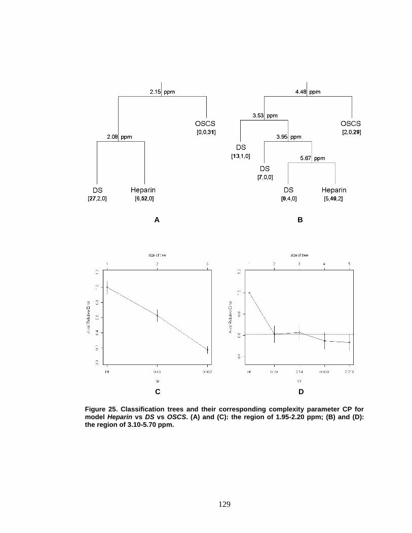
129
A B
C D
Figure 25. Classification trees and their corresponding complexity parameter CP for model Heparin vs DS vs OSCS. (A) and (C): the region of 1.95-2.20 ppm; (B) and (D): the region of 3.10-5.70 ppm.

130
(Heparin + DS) group was split into the DS and Heparin classes solely by the
chemical shift 2.08 ppm. Both of these terminal nodes contain
misclassifications. The DS node contains two Heparin samples, while the
Heparin node contains six DS samples. The classification rates, summarized
in Table 16, were 93.2% (110/118) for the training set (8 misclassifications)
and 90.0% (54/60) for the test set (6 misclassifications).
When modeling the data set of the 3.10-5.70 ppm region, the resulting tree
was slightly more complex, consisting of five terminal nodes (Figure 25B).
The variables splitting the data are 3.53, 3.95, 4.48 and 5.67 ppm. Variable
Table 16. Model Parameters and Classification Rates for CART
__________________________________________________________________________________
Model Region Nodes Variables Training Test
ppm ppm % % __________________________________________________________________________________
Heparin vs DS 1.95 - 5.70 2 2.08 90.8 (79/87) 88.9 (40/45)
1.95 - 2.20 2 2.08 90.8 (79/87) 88.9 (40/45)
3.10 - 5.70 3 3.53, 3.86 83.9 (73/87) 80.0 (36/45) Heparin vs OSCS 1.95 - 5.70 2 2.15 100 (85/85) 100 (43/43)
1.95 - 2.20 2 2.15 100 (85/85) 100 (43/43)
3.10 - 5.70 2 4.48 97.6 (83/85) 97.7 (42/43)
Heparin vs [DS + OSCS] 1.95 - 5.70 3 2.08, 2.15 91.5 (108/118) 90.0 (54/60)
1.95 - 2.20 3 2.08, 2.15 91.5 (108/118) 90.0 (54/60)
3.10 - 5.70 5 3.53, 3.95, 4.48, 5.67 89.8 (106/118) 78.3 (47/60)
3.10 - 5.70 4 3.53, 3.95, 4.48 88.1 (104/118) 83.3 (50/60) Heparin vs DS vs OSCS 1.95 - 5.70 3 2.08, 2.15 93.2 (110/118) 90.0 (54/60)
1.95 - 2.20 3 2.08, 2.15 93.2 (110/118) 90.0 (54/60)
3.10 - 5.70 5 3.53, 3.95, 4.48, 5.67 88.1 (104/118) 80.0 (48/60)
3.10 - 5.70 4 3.53, 3.95, 4.48 86.4 (102/118) 85.0 (51/60) __________________________________________________________________________________
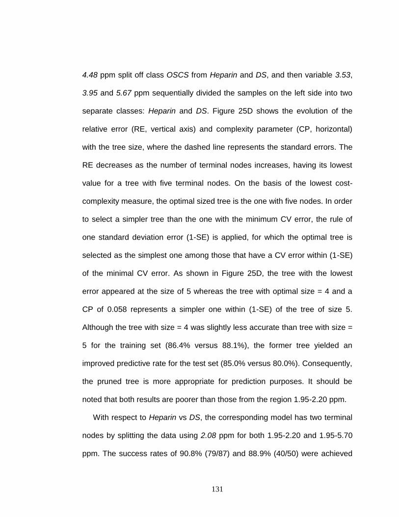
131
4.48 ppm split off class OSCS from Heparin and DS, and then variable 3.53,
3.95 and 5.67 ppm sequentially divided the samples on the left side into two
separate classes: Heparin and DS. Figure 25D shows the evolution of the
relative error (RE, vertical axis) and complexity parameter (CP, horizontal)
with the tree size, where the dashed line represents the standard errors. The
RE decreases as the number of terminal nodes increases, having its lowest
value for a tree with five terminal nodes. On the basis of the lowest cost-
complexity measure, the optimal sized tree is the one with five nodes. In order
to select a simpler tree than the one with the minimum CV error, the rule of
one standard deviation error (1-SE) is applied, for which the optimal tree is
selected as the simplest one among those that have a CV error within (1-SE)
of the minimal CV error. As shown in Figure 25D, the tree with the lowest
error appeared at the size of 5 whereas the tree with optimal size = 4 and a
CP of 0.058 represents a simpler one within (1-SE) of the tree of size 5.
Although the tree with size = 4 was slightly less accurate than tree with size =
5 for the training set (86.4% versus 88.1%), the former tree yielded an
improved predictive rate for the test set (85.0% versus 80.0%). Consequently,
the pruned tree is more appropriate for prediction purposes. It should be
noted that both results are poorer than those from the region 1.95-2.20 ppm.
With respect to Heparin vs DS, the corresponding model has two terminal
nodes by splitting the data using 2.08 ppm for both 1.95-2.20 and 1.95-5.70
ppm. The success rates of 90.8% (79/87) and 88.9% (40/50) were achieved
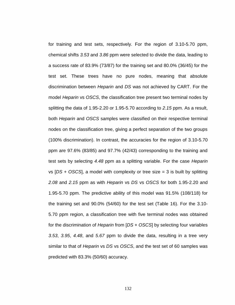
132
for training and test sets, respectively. For the region of 3.10-5.70 ppm,
chemical shifts 3.53 and 3.86 ppm were selected to divide the data, leading to
a success rate of 83.9% (73/87) for the training set and 80.0% (36/45) for the
test set. These trees have no pure nodes, meaning that absolute
discrimination between Heparin and DS was not achieved by CART. For the
model Heparin vs OSCS, the classification tree present two terminal nodes by
splitting the data of 1.95-2.20 or 1.95-5.70 according to 2.15 ppm. As a result,
both Heparin and OSCS samples were classified on their respective terminal
nodes on the classification tree, giving a perfect separation of the two groups
(100% discrimination). In contrast, the accuracies for the region of 3.10-5.70
ppm are 97.6% (83/85) and 97.7% (42/43) corresponding to the training and
test sets by selecting 4.48 ppm as a splitting variable. For the case Heparin
vs [DS + OSCS], a model with complexity or tree size = 3 is built by splitting
2.08 and 2.15 ppm as with Heparin vs DS vs OSCS for both 1.95-2.20 and
1.95-5.70 ppm. The predictive ability of this model was 91.5% (108/118) for
the training set and 90.0% (54/60) for the test set (Table 16). For the 3.10-
5.70 ppm region, a classification tree with five terminal nodes was obtained
for the discrimination of Heparin from [DS + OSCS] by selecting four variables
3.53, 3.95, 4.48, and 5.67 ppm to divide the data, resulting in a tree very
similar to that of Heparin vs DS vs OSCS, and the test set of 60 samples was
predicted with 83.3% (50/60) accuracy.

133
Analysis of the above results reveals that the predictive and discrimination
ability is much better with trees built from 1.95-2.20 and 1.95-5.70 ppm than
from 3.10-5.70 ppm. In addition, the discrimination results are exactly the
same using the entire region 1.95-5.70 ppm as using the local region 1.95-
2.20 ppm. Although 1.95-5.70 ppm region contains more variables (74) and
many more details in terms of chemical shifts, the CART model selected only
2.08 and 2.15 ppm as the splitting variables and ignored the 3.10-5.70 ppm
region entirely, suggesting the N-acetyl methyl proton chemical shifts (1.95-
2.20 ppm) play a critical role in discriminating heparin from its impurities and
contaminants for the CART model.
4.2.6 Artificial Neural Networks
A three-layer feed-forward network trained with a back propagation
algorithm was investigated to optimize separation between pure, impure and
contaminated heparin samples, and to build predictive models for class
identification. The input layer contained as many neurons as the independent
variables of the dataset, which are the chemical shifts with numbers of 9, 65
and 74 for the data sets of 1.95-2.20, 3.10-5.70 and 1.95-5.70 ppm,
respectively, and the output corresponded to the four classes Heparin, DS,
OSCS and [DS + OSCS]. The number of neurons in the hidden layer was
varied to assess its influence on network performance. Too few hidden
neurons will lead to poor generalization and the built model becomes
unstable, whereas if too many hidden neurons are used, the neural network

134
will overfit the training data. The sigmoid transfer function was exclusively
employed for activation in both hidden and output layers. The output from the
ANN is a prediction of the class membership in the samples of each class,
consisting of a matrix Ŷ with the same dimensions as the dependent variable
Y that contains the binary values of 1 or 0 for each class and comprises as
many columns as there are classes. The numeric value of element ŷij in Ŷ is
in an interval between 0 and 1, which can be regarded as an estimate of the
probability for assigning the ith sample to the jth class. If the output value is
close to 1, then the test sample is ascribed to the modeled class while the
sample is assigned to other classes if the value is close to 0.
For ANN, a commonly used error function is the cross entropy or deviance
defined in Equation 44 [36]:
Minimize: ij
n
i
k
j
ij yy ˆlogˆ1 1
(44)
Since ANN is very sensitive to overfitting, a regularization term, called weight
decay, is introduced. The modified criterion is given by Equation 45:
Minimize:
2
1 1
)(ˆlogˆ parametersyy ij
n
i
k
j
ij (45)
where “parameters” represents the values of all parameters that are used in
the ANN training. Therefore, the second term takes into account the
magnitude of all the parameters. The magnitude of the adjusting parameter λ
controls how much the constraint of shrinking the parameters should be
addressed. When the value of λ is zero (i.e., no weight decay) or small, the

135
boundary or edge between classes is rough or non-smooth, leading to
overfitting of the model, while a smoother boundary is yielded as the weight
decay increases.
For ANN classification, the number of hidden units and the weight decay
need to be optimized, which can be done through cross validation. Figure 26
shows the relationship between the misclassification rate of the classification
and the decay weight and the number of neurons for the training set, test set
and 10-fold CV process for Heparin vs DS vs OSCS with the data set of 1.95-
5.70 ppm. In order to investigate the influence of the size of neurons in the
hidden layer on the prediction accuracy, ANNs with neuron numbers ranging
from 3 to 30 were developed with the weight decay fixed at 0.1. The
prediction results are plotted as a function of the size of hidden units in Figure
26A that shows that 9 neurons in the hidden layer are optimal. The
dependency of the error rate on the weight decay λ for 9 hidden units is
depicted in Figure 26B.
The optimal values of these parameters and the results of the ANNs
analysis, performed by combining in various types of input data, are
presented in Table 17. For Heparin vs DS vs OSCS, with the optimal settings
of λ = 0.075 and neurons = 6, this specific ANN showed a classification rate
of 96.6% (114/118) and a prediction accuracy was 91.7% (55/60) with only
five samples misclassified in the test set for the 1.95-2.20 range. The
prediction accuracy for the training set and test set corresponded to 95.8%

136
A
B
Figure 26. The variations of misclassification errors from ANN with the hidden units and weight decay for the model Heparin vs DS vs OSCS for the data set in the 1.95-5.70 ppm range. (A) Fixing weight decay with λ = 0.1; (B) Fixing the number of hidden units at 9.

137
Table 17. Model Parameters and Classification Rates for ANN __________________________________________________________________________________
Model Region Hidden size Weight decay Training Test
ppm λ % % __________________________________________________________________________________
Heparin vs DS 1.95 - 5.70 9 5.0 × 10⁻¹
95.4 (83/87) 86.7 (39/45)
1.95 - 2.20 6 5.0 × 10⁻²
97.7 (85/87) 88.9 (40/45)
3.10 - 5.70 9 3.0 × 10⁻¹
96.6 (84/87) 84.4 (38/45) Heparin vs OSCS 1.95 - 5.70 9 1.0 × 10
-1 100 (85/85) 100 (43/43)
1.95 - 2.20 6 2.0 × 10⁻²
100 (85/85) 100 (43/43)
3.10 - 5.70 9 1.0 × 10⁻¹
100 (85/85) 100 (43/43) Heparin vs [DS + OSCS] 1.95 - 5.70 9 2.5 × 10
-1 94.9 (112/118) 91.7 (55/60)
1.95 - 2.20 6 3.0 × 10⁻²
99.2 (117/118) 91.7 (55/60)
3.10 - 5.70 9 2.0 × 10⁻¹
99.2 (117/118) 90.0 (54/60) Heparin vs DS vs OSCS 1.95 - 5.70 9 9.0 × 10
-1 95.8 (113/118) 88.3 (53/60)
1.95 - 2.20 6 7.5 × 10⁻²
96.6 (114/118) 91.7(55/60)
3.10 - 5.70 9 8.0 × 10⁻¹
93.2 (110/118) 86.7(52/60) __________________________________________________________________________________
(113/118) and 88.3% (53/60) for the 1.95-5.70 range and, similarly, with
93.2% (110/118) and 86.7% (52/60) for the 3.10-5.70 ppm range. This can be
shown by the number of misclassified samples indicated in Table 17. For
Heparin vs OSCS, the ANN model classified all members of the training and
tests sets correctly with 100% prediction accuracy. The prediction rates for
the Heparin vs DS model for the three regions are very close with 95.4-97.7%
for the training set and 84.4-88.9% for the test set. For the Heparin vs [DS +
OSCS] model, the prediction rates of the various networks were quite similar
at 90.0-91.7% for the three regions as summarized in Table 17. In general,
the performance of the models was slightly better for those built from the
1.95-2.20 ppm than from either the 3.10-5.70 or 1.95-5.70 ppm regions.

138
4.2.7 Support Vector Machine
Using the same training and test sets as for CART and ANN, the SVM
algorithm with the non-linear soft margin was employed to build classification
models. For SVM classification with the RBF kernel, the optimization requires
to specify two parameters, i.e., the width of the kernel function γ and the
regularization parameter C. Their combination determines the boundary
complexity and thus the classification performance, i.e., prediction ability.
Cross-validation (CV) is widely used to determine the parameters for
evaluating the performance of the model and minimizing the risk of overfitting.
The parameters C and γ are optimized by the user, and the optimal values
are obtained by performing an exhaustive grid search with 10-fold CV on the
training set using their various combinations. The set of C and γ values giving
the highest percentage accuracy or the lowest error rate is selected for further
analysis. In this study, a wide range of γ and C values were tuned
simultaneously in a 9 × 9 grid of 81 possible combinations for C from 1 to 108
and γ from 10−8 to 1. After all the combinations have been searched, a
contour plot is created in decimal logarithmic scales, which indicates the
prediction accuracy or classification error. Figure 27 presents the optimization
grids in terms of cross validation classification rate for the models Heparin vs
DS vs OSCS and Heparin vs OSCS. The two coarse grid plots of γ and C
values delineate regions where the optimal parameter settings might be
located. The two deep red “islands” in Figure 27A correspond to the lowest

139
prediction error for Heparin vs DS vs OSCS, reflecting the difficulty in tuning
the γ and C values to achieve optimal discrimination of Heparin, DS and
OSCS. In contrast, the large red stripe in Figure 27B reflects the relative ease
in tuning the γ and C values for optimal discrimination of Heparin vs OSCS. In
order to obtain high resolution, this range of γ and C values are further refined
to achieve the final SVM model. The SVM model of Heparin vs DS vs OSCS
with the optimum values C = 6.0 × 10⁴ and γ = 1.0 × 10⁻³ for 1.95-5.70 ppm
gave the best classification performance. For Heparin vs OSCS, the optimal
parameter settings C = 1.0 × 10³ and γ = 1.0 × 10⁻⁴ led to perfect
discrimination.
Using the optimal paired values of γ and C, the results from SVM are
summarized in Table 18. The prediction accuracy is > 90% in all cases for the
samples for all data sets. A larger number of samples were classified
correctly, and the models generally presented few (< 3-5) misclassifications. It
is worth noting that SVM achieved nearly identical results for both the 1.95-
2.20 ppm and 3.10-5.70 ppm regions, giving credence to its ability to
differentiate even subtle structural differences between pure, impure, and
contaminated heparin. In contrast, visual inspection of the Heparin, DS, and
OSCS spectra (Figure 13) clearly reveals distinctions in the 1.95-2.20 ppm
region but not in the 3.10-5.70 ppm region.

140
A
B
Figure 27. Contour plots in decimal logarithmic scales obtained from 9 × 9 grid search of the optimal values of γ and C for the SVM model. (A) Heparin vs DS vs OSCS for the 1.95-5.70 ppm region; (B) Heparin vs OSCS for the 1.95-5.70 ppm region.

141
Table 18. Model Parameters and Classification Rates for SVM __________________________________________________________________________________
Model Region C γ Training Test
ppm % % __________________________________________________________________________________
Heparin vs DS 1.95 - 5.70 2.0 × 10
3 1.0 × 10
-4 97.7 (85/87) 91.1 (41/45)
1.95 - 2.20 1.0 × 10⁴ 1.0 × 10
-3 96.6 (84/87) 93.3 (42/45)
3.10 - 5.70 1.8 × 10⁴ 1.0 × 10
-4 97.7 (85/87) 93.3 (42/45)
Heparin vs OSCS 1.95 - 5.70 1.0 × 10
3 1.0 × 10
-4 100 (85/85) 100 (43/43)
1.95 - 2.20 1.0 × 10³ 1.0 × 10
-4 100 (85/85) 100 (43/43)
3.10 - 5.70 1.0 × 10³ 1.0 × 10
-4 100 (85/85) 100 (43/43)
Heparin vs [DS + OSCS] 1.95 - 5.70 8.0 × 10
4 1.0 × 10
-5 98.3 (116/118) 95.0 (57/60)
1.95 - 2.20 1.0 × 10⁷ 2.0 × 10
-4 97.5 (115/118) 95.0 (57/60)
3.10 - 5.70 1.0 × 10⁵ 1.8 × 10
-5 98.3 (116/118) 95.0 (57/60)
Heparin vs DS vs OSCS 1.95 - 5.70 6.0 × 10
4 1.0 × 10
-3 97.5 (115/118) 95.0 (57/60)
1.95 - 2.20 2.0 × 10⁵ 1.0 × 10
-3 99.2 (117/118) 95.0 (57/60)
3.10 - 5.70 1.5 × 10⁵ 1.0 × 10
-5 98.3 (116/118) 95.0 (57/60)
__________________________________________________________________________________
4.2.8 Analysis of Misclassifications
As shown in Tables 16, 17 and 18, the predictive abilities of the
classification models built from CART, ANN and SVM were outstanding in
differentiating Heparin from DS and OSCS with few errors. In particular,
higher predictive accuracies or fewer misclassifications were attained for the
Heparin vs OSCS model than for Heparin vs DS, Heparin vs [DS + OSCS]
and Heparin vs DS vs OSCS models. While all three pattern recognition
approaches were able to completely discriminate Heparin and OSCS with
success rates of 100% under optimal conditions, for the other models it can
be seen by cross comparison from Tables 16 to 18 that using the same input

142
variables, the model generated from the SVM algorithm consistently
outperformed ANN, which in turn marginally outperformed CART. When the
entire chemical shift region was divided into two subsets (1.95-2.20 and 3.10-
5.70 ppm), better results were achieved for the former than the latter region.
The sole exception was SVM, which achieved nearly identical results from
both regions. SVM performed better in every aspect, as can be appreciated
by comparing the misclassified rates in Tables 16-18. Taking the Heparin vs
DS vs OSCS model for the region of 3.10-5.70 ppm as an example, the
success rates of the training set and test set were appreciably higher for SVM
(98.3% and 95.0%) than for CART (86.4% and 85.0%) and ANN (93.2% and
86.7%).
Tables 19-21 summarize the results of the classification matrices
evaluated by means of both training and test sets in the region of 1.95-5.70
ppm. All of the misclassified samples were between Heparin and DS: several
samples belonging to Heparin were predicted as DS, while some DS samples
were predicted as Heparin. Using SVM, only one Heparin sample was
misclassified as DS and three DS samples were misclassified as Heparin for
the Heparin vs DS model in the test set (Table 19). Misclassification of
Heparin as DS occurred only once and DS as Heparin twice for the Heparin
vs [DS + OSCS] model (Table 20). The same result occurred for the threefold
Heparin vs DS vs OSCS model, that is, SVM produced a total of three
misclassifications (Table 21).

143
When examining the misclassified samples, it was noted that in most
cases, these misclassifications occurred when the DS content of the sample
ranged from 0.90% to 1.20%, i.e., they were close to the DS = 1.0% impurity
limit defining the Heparin and DS classes, and it is hard to distinguish from
each other due to the similarity in the 1H NMR spectral patterns of Heparin
and DS samples on the borderline. When removing these borderline samples
from the data set, it was found that the overall performance of the model was
greatly improved and much better results with very few misclassifications
were achieved, especially for the SVM model, where only one sample was
misclassified in the test set (Tables 19-21).
Table 19. Classification Matrices for the Heparin vs DS Model in 1.95-5.70 ppm Region __________________________________________________________________________________
All samples After removing borderline samples ________________________ _______________________________
Training set Test set Training set Test set Heparin DS Heparin DS Heparin DS Heparin DS __________________________________________________________________________________
CART Heparin 52 6 25 2 48 3 23 0
DS 2 27 3 15 2 23 2 13
ANN Heparin 52 2 27 5 50 0 25 2
DS 2 31 1 12 0 26 0 11
SVM Heparin 53 1 27 3 50 0 25 1
DS 1 32 1 14 0 26 0 12 __________________________________________________________________________________

144
Table 20. Classification Matrices for the Heparin vs [DS + OSCS] Model
in the 1.95-5.70 ppm Region __________________________________________________________________________________
All samples After removing borderline samples ______________________________ _______________________________
Training set Test set Training set Test set Hep [DS + OSCS] Hep [DS + OSCS] Hep [DS + OSCS] Hep [DS + OSCS]
__________________________________________________________________________________
CART Heparin 49 5 24 2 46 3 23 0
[DS + OSCS] 5 59 4 30 4 54 2 28
ANN Heparin 52 4 27 4 50 0 24 2
[DS + OSCS] 2 60 1 28 0 57 1 26
SVM Heparin 52 1 27 2 50 0 25 1
[DS + OSCS] 2 63 1 30 0 57 0 27
__________________________________________________________________________________
Table 21. Classification Matrices for the Heparin vs DS vs OSCS Model
in the 1.95-5.70 ppm Region __________________________________________________________________________________
All samples After removing borderline samples ________________________________ ________________________________
Training set Test set Training set Test set Hep DS OSCS Hep DS OSCS Hep DS OSCS Hep DS OSCS __________________________________________________________________________________
CART Heparin 52 6 0 25 2 0 48 3 0 23 1 0
DS 2 27 0 3 14 0 2 23 0 2 12 0
OSCS 0 0 31 0 1 15 0 0 31 0 0 15
ANN Heparin 52 3 0 25 5 0 50 0 0 25 2 0
DS 2 30 0 3 12 0 0 26 0 0 11 0
OSCS 0 0 31 0 0 15 0 0 31 0 0 15
SVM Heparin 53 0 0 27 2 0 50 1 0 25 1 0
DS 1 33 0 1 15 0 0 25 0 0 12 0
OSCS 0 0 31 0 0 15 0 0 31 0 0 15 __________________________________________________________________________________

145
4.2.9 Classification Analysis of Heparin Spiked with other GAGs
Heparin APIs may contain GAG impurities other than dermatan sulfate
(DS), such as chondroitin sulfate A (CSA) and heparan sulfate (HS), and
other possible synthetic oversulfated contaminants that can mimic the
functions of heparin, could be found in heparin lots. In order to assess the
capability of the developed models to discriminate and detect a wide range of
potential GAG-like impurities and contaminants previously unseen in the
heparin samples, a series of blends was prepared by spiking heparin APIs
with native impurities CSA, DS and HS, as well as their partially- or fully-
oversulfated (OS) versions OS-CSA (i.e., OSCS), OS-DS, OS-HS and OS-
heparin at the 1.0%, 5.0% and 10.0% weight percent levels [15], and the
resulting multivariate statistical models were used to test their class
assignations for the Heparin vs DS vs OSCS model. The blend samples are
highly diverse in composition when compared to the clearly defined Heparin,
DS and OSCS classes, since they contain multiple components with varying
degrees of sulfation and concentration from 1% to 10% as shown in Table 22.
For exploratory purposes, agglomerative hierarchical cluster analysis
(HCA) was performed on the 30 blend samples. As an unsupervised
technique, HCA describes the nearness between objects, identifies specific
differences, finds natural groupings of the data set, and allows the
visualization of the relationships between objects in the form of a dendrogram
[112, 115, 146]. The procedure starts by setting each object in its own cluster,

146
and then two objects closest together are joined, followed by the next step in
which either a third object joins the just formed cluster, or two clusters join
together into a new cluster. Each step yields clusters with a number less than
the previous step. The iterative procedure repeats until all objects are merged
into a single cluster. HCA analysis was implemented using the Euclidean
distance for measuring the similarity among blend samples with average
linkage for merging the clusters. Figure 28 depicts the hierarchical clustering
of the blend samples in the 1.95-5.70 ppm region. From this dendrogram, two
distinct clusters can be observed, which were formed according to the content
of GAGs. The cluster on the left-side included samples with the low content of
GAGs (1%), while the high content of GAGs (i.e., 5% and 10%) comprised
the right-side cluster which consists of two sub-clusters, one is a cluster of the
native GAGs, i.e., CSA (B1 and B2), DS (B4 and B5) and HS (B7 and B8),
and another is made of oversulfated GAGs, where the samples with the same
GAG composition lay close to each other and clustered in pair.
The test results obtained in the identification of the blend samples using
the resulting models from CART, ANN and SVM are summarized in Table 22.
Blend samples B28-30 (blank or control samples), B4-6 (DS) and B10-12
(OS-CSA) correspond to the classes Heparin, DS and OSCS, respectively.
As expected, all of them were correctly classified into their respective classes.
All other blends, by nature, don‟t belong to any the designated class, but they
have to be assigned to a class. As can be seen, some blends containing low
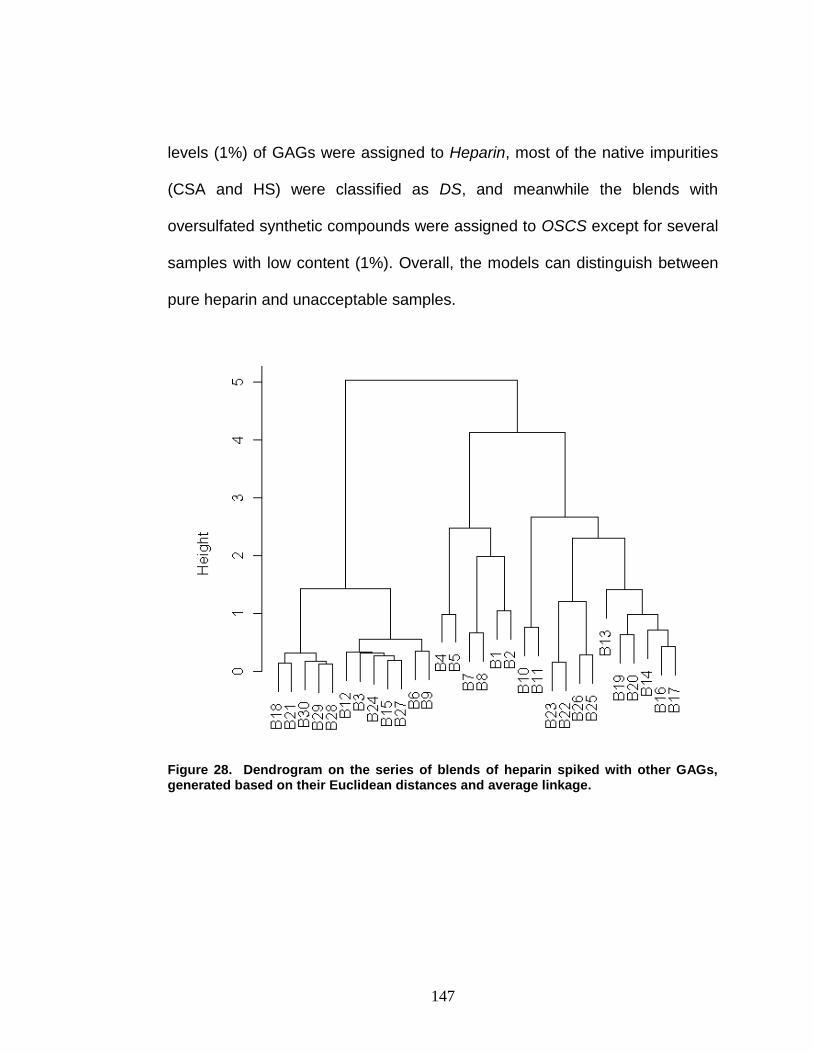
147
levels (1%) of GAGs were assigned to Heparin, most of the native impurities
(CSA and HS) were classified as DS, and meanwhile the blends with
oversulfated synthetic compounds were assigned to OSCS except for several
samples with low content (1%). Overall, the models can distinguish between
pure heparin and unacceptable samples.
Figure 28. Dendrogram on the series of blends of heparin spiked with other GAGs, generated based on their Euclidean distances and average linkage.

148
Table 22. Compositions of the Series of Blends of Heparin Spiked with other GAGs and
Test Results for Classification from SVM, CART and ANN in the 1.95-5.70 ppm Region __________________________________________________________________________________
ID GAGs Content (%) SVM CART ANN ___________________________________________
Classified as Heparin (H), DS (D) or OSCS (O) __________________________________________________________________________________
B1 CSA 10 D D D B2 CSA 5 D D D B3 CSA 1 D D D
B4 DS 10 D D D B5 DS 5 D D D B6 DS 1 D D D
B7 HS 10 D D D B8 HS 5 D D D B9 HS 1 H H H
B10 FS-CSA 10 O O O B11 FS-CSA 5 O O O B12 FS-CSA 1 O D D
B13 FS-DS 10 O O O B14 FS-DS 5 O O O B15 FS-DS 1 D D D
B16 OS-HS 10 O O O B17 OS-HS 5 O O O B18 OS-HS 1 H H H
B19 OS-Hep 10 O O O B20 OS-Hep 5 O O O B21 OS-Hep 1 H H H
B22 PS-CSA#1 10 O O O B23 PS-CSA#1 5 O O D B24 PS-CSA#1 1 D H H
B25 PS-CSA#2 10 O O O B26 PS-CSA#2 5 O O D B27 PS-CSA#2 1 D H H
B28 Blank - H H H B29 Blank - H H H B30 Blank - H H H __________________________________________________________________________________
CSA: chondroitin sulfate A; DS: dermatan sulfate; HS: heparan sulfate; FS: fully sulfated;
OS: oversulfated; PS: partially sulfated; Blank: control (pure heparin sample). The weight
percent sulfur for PS-CSA#1 and PS-CSA#2 is 11.01% and 11.14%, respectively.

149
4.3 Class Modeling for Discriminating Heparin Samples
Previously we explored the ability of pure classification methods, i.e.,
principal component analysis (PCA), partial least squares discriminant
analysis (PLS-DA), linear discriminant analysis (LDA), k-nearest neighbor
(kNN), classification and regression tree (CART), artificial neural network
(ANN), and support vector machine (SVM), to distinguish between pure,
impure and contaminated heparin samples based on evaluation of their 1H
NMR spectra. Class modeling techniques represent a substantially different
modeling strategy. Whereas pure discriminating methods focus on the
dissimilarity between classes, class modeling approaches emphasize the
similarity within each class. In this section, soft independent modeling of class
analogy (SIMCA) and unequal class modeling (UNEQ) were applied to
differentiate heparin samples that contain varying amounts of dermatan
sulfate (DS) impurities and oversulfated chondroitin sulfate (OSCS)
contaminants. The two methods enable the construction of individual models
for each class and the determination of the modeling ability of each variable in
a class.
4.3.1 SIMCA Analysis
In SIMCA, each class is modeled separately using principal component
analysis (PCA). Class boundaries which define the range of acceptable
samples at a selected confidence level are built around the PC model that
encloses the internal space. SIMCA is able to indicate the discriminant power

150
and modeling power for each variable when defining the similarity among the
members of a class of samples.
4.3.1.1 Analysis of Pure, Impure and Contaminated Heparin Samples
The SIMCA model was developed using a set of 1H NMR spectral data
with 168 samples corresponding to 72 heparin samples, 50 DS/heparin
samples and 46 OSCS/heparin samples with 74 variables. As defined above,
three classes, i.e., Heparin, DS, and OSCS were considered. An additional
fourth class, namely [DS + OSCS], was included to characterize samples that
contained DS > 1.0% or OSCS > 0%. For each class, only components with
eigenvalues greater than unity were employed to build the model. The
numbers of PCs used for the class models were twelve for the class Heparin,
and nine each for the DS, OSCS and [DS + OSCS] classes, accounting for
98.4, 99.3, 99.4, and 98.7% of the total variance, respectively. The results of
SIMCA modeling after separate category autoscaling and column centering
are reported in Table 23. It was observed that 16 of the 72 Heparin, 13 of the
50 DS, 7 of the 46 OSCS and 20 of the 96 [DS + OSCS] samples were
erroneously rejected by their specific category models by the SIMCA F-test at
the 95% confidence level, resulting in a SENS of 77.8%, 74.0%, 84.8% and
79.2% for the four classes, respectively. The class models built using SIMCA
exhibited high SPEC particularly for the OSCS class model. Both Heparin and
DS rejected all samples in OSCS, leading to a SPEC of 100%. OSCS also
rejected all samples in Heparin and accepted only one sample in DS. In

151
addition, the Heparin class model accepted the same five DS samples from
both DS and [DS + OSCS] classes; hence, the SPECs of Heparin for DS and
for [DS + OSCS] were 90.0% (45/50) and 94.8% (91/96), respectively. The
DS content in these five samples was in the range 1.06% to 1.20%, i.e., they
were nearby the borderline of the 1.0% acceptance criterion. The same
observation was ascribed as the cause of misclassifications in the previous
work [16, 147]. On the other hand, the DS and [DS + OSCS] class models
accepted 13 and 32 Heparin samples, respectively, corresponding to SPEC
values of 81.9% and 55.6%, respectively. The low SPEC value of the [DS +
OSCS] class model was due to its difficulty in discriminating Heparin samples
from DS samples in cases where the DS content was nearby the 1.0%
acceptance criterion for DS.
Table 23. Sensitivity and Specificity from SIMCA Modeling
__________________________________________________________________________________
Model Number Explained Sensitivity (%) Specificity (%) of PCs variance (%) __________________________________________________________________________________
Heparin 12 98.4 77.8 (56/72) 90.0 (45/50) for DS;
100 (46/46) for OSCS;
94.8 (91/96) for [DS + OSCS].
DS 9 99.3 74.0 (37/50) 81.9 (59/72) for Heparin;
100 (46/46) for OSCS.
OSCS 9 99.4 84.8 (39/46) 100 (72/72) for Heparin;
98.0 (49/50) for DS.
[DS + OSCS] 9 98.7 79.2 (76/96) 55.6 (40/72) for Heparin.
__________________________________________________________________________________

152
The results of class modeling can be displayed by means of Coomans
plots, which are a useful tool for visualizing the groupings [93, 99, 148]. In a
Coomans plot, two classes are drawn against one another, and each
category is plotted as a rectangle whose boundary corresponds to the
confidence limit defined by the class space. The distance of each sample
from both categories is measured by the coordinates in the axes [80, 97,
135]. The plot is divided into four areas by the boundary of 95% confidence
level for both categories. The samples accepted by only one model fall in two
areas of the Coomans plot: one is the left upper rectangle and another is the
right bottom rectangle. Samples located in the lower-left corner area, where
the two categories overlap, are accepted by both of the two classes. A
sample whose distance is beyond the critical limit for the class model is
rejected as an outlier for that specific class. Consequently, it is plotted outside
the area defining the class model. Samples rejected by both models are
plotted in the upper-right square.
The Coomans plots for different pairs of classes are displayed in Figure
29, in which each sample is represented by its category index. The
distribution of the samples from these models at the critical distance for 95%
confidence is shown. Most of the samples were correctly accepted by their
respective classes, with only few samples plotted beyond their critical limits.
Figure 29A shows the Coomans plot for the Heparin and OSCS classes,
which are located in the upper left quadrant and lower right quadrant of

153
A B
C D
Figure 29. Coomans plots for SIMCA class modeling. (A) Heparin vs OSCS; (B) Heparin vs DS; (C) Heparin vs [DS + OSCS]; (D) DS vs OSCS.

154
the plot, respectively. All the OSCS samples are clustered at the right side,
forming a tight group, and all are far from the lower left corner. Meanwhile no
Heparin sample fell into the bottom box. All of the OSCS samples were
completely separated from the Heparin class without any overlap between the
two classes, indicating 100% successful discrimination.
The Coomans plot for the Heparin and DS classes is shown in Figure 29B.
The upper left zone corresponds to the samples accepted by the Heparin
class model while the bottom right zone corresponds to the samples accepted
by the DS class model. Heparin samples with low DS content are far from the
bottom box, i.e., the DS class model, while samples with DS content close to
1.0% are located near or within the lower left square. One sample (with %DS
= 1.04) was accepted by the DS model and 12 samples (with %DS = 0.80-
1.02) appear in the overlapping area. Although 13 DS samples were rejected
by the DS class model, all of these samples fell close to the boundary.
Samples with high DS content are situated on the right side while samples
with low DS content are very close to the Heparin model. The samples
situated in the lower left square of the diagram are accepted by both models.
Unsurprisingly, a certain degree of overlap occurred between the models of
these two classes. The Heparin class model accepted five DS samples, while
the DS class model accepted 13 Heparin samples as indicated in the left
bottom square.

155
The Coomans plot for the Heparin and [DS + OSCS] classes is shown in
Figure 29C. Similar to Figure 29A and 29B, Figure 29C demonstrates that all
OSCS samples are located on the right side and five DS samples are in the
lower left square. Of the 72 samples belonging to the Heparin class, 32 are
plotted in the lower left quadrant belonging to both classes, revealing the low
degree of specificity of the [DS + OSCS] class model for the Heparin class.
In the Coomans plot for the DS and OSCS classes (Figure 29D), all of the
OSCS samples were significantly distant from the region of the left rectangle
corresponding to the DS class model and far from the critical distance of the
DS class model. No OSCS samples fell in the region for the DS model, thus
the specificity of DS with respect to OSCS was 100%. Likewise, the OSCS
model accepted only 1 of the 50 DS samples corresponding to 98%
specificity. Overall, excellent separation was achieved between the Heparin
and OSCS classes and between the DS and OSCS classes.
In SIMCA, a sample is classified according to its analogy with samples
belonging to a class defined by principal components (PCs). Classification is
carried out based on the orthogonal distance of the sample to the hyperplane
of the class model defined by the first few PCs. The classification
performance is evaluated in terms of prediction ability. Validation of the class
models was performed using a full leave-one-out cross-validation (LOO-CV)
approach, which recalculates the local models after each sample is
sequentially excluded from the model [99]. Training and prediction rates were

156
computed as the average of the classification rates for each class,
corresponding to the success rate in classifying the training set samples and
the success rate in classifying the test set samples. The results obtained for
the training and test sets are summarized in Table 24, recorded as the
classification matrix of the model indicating the correct predictions for each
class. The success rates for the training and test sets were 99.2% and 92.4%
for Heparin vs OSCS and 94.3% and 81.1% for Heparin vs DS. The number
of misclassifications was unevenly distributed among the different classes,
with higher number of errors occurring in the Heparin and DS classes. The
OSCS samples were sufficiently distant from the Heparin and DS class
models, and consequently none of the OSCS samples were misclassified as
either Heparin or DS. The OSCS samples were classified perfectly (no
misclassifications) both in the training and the validation phases. However,
this was not the case for other SIMCA class models. For Heparin vs OSCS, 3
of the 72 Heparin samples were misclassified as OSCS. For DS vs OSCS, 11
of the 50 DS samples were misclassified as OSCS.
Given the similarity in the 1H NMR spectra of heparin and DS, several
samples were misclassified for Heparin vs DS. Fifteen of the 72 Heparin
samples were misclassified as DS while 8 of the 50 DS samples were
misclassified as Heparin. A great number of Heparin samples were
misclassified for Heparin vs [DS + OSCS], in which 29 of the 72 Heparin
samples were assigned to [DS + OSCS] whereas 7 of the 96 [DS + OSCS]

157
samples assigned to Heparin, all of these 7 samples belonging to the DS
class.
Table 24. Classification Matrices and Success Rates from SIMCA Class Modeling
__________________________________________________________________________________
Model Training Prediction __________________________________________________________________________________
Heparin vs DS Hep DS Rate (%) Hep DS Rate (%)
Hep 68 4 94.4 57 15 79.2
DS 3 47 94.0 8 42 84.0
Total - - 94.3 - - 81.1
Heparin vs OSCS Hep OSCS Rate (%) Hep OSCS Rate (%)
Hep 71 1 98.6 63 9 87.5
OSCS 0 46 100 0 46 100
Total - - 99.2 - - 92.4
Heparin vs [DS + OSCS] Hep [DS + OSCS] Rate (%) Hep [DS + OSCS] Rate (%)
Hep 68 4 94.4 47 25 65.3
[DS + OSCS] 7 89 92.7 9 87 90.6
Total - - 93.5 - - 79.8
DS vs OSCS DS OSCS Rate (%) DS OSCS Rate (%)
DS 49 1 98.0 39 11 78.0
OSCS 0 46 100 0 46 100
Total - - 99.0 - - 88.5
Heparin vs DS vs OSCS Hep DS OSCS Rate (%) Hep DS OSCS Rate (%)
Hep 54 17 1 75.0 45 22 5 62.5
DS 0 49 1 98.0 5 36 9 72.0
OSCS 0 0 46 100 0 0 46 100
Total - - - 88.7 - - - 75.6 __________________________________________________________________________________

158
With regard to the three-class system Heparin vs DS vs OSCS, OSCS
yielded a 100% success rate in prediction ability on the test set. On the other
hand, 5 and 22 of the 72 samples from the Heparin class were misclassified
to OSCS and DS, respectively, while 5 and 9 of the 50 samples from the DS
class were misclassified to Heparin and OSCS, respectively. The expected
poor prediction ability of both Heparin and DS resulted in a modest overall
classification rate of 75.6%.
As a highly informative multivariate analysis technique, SIMCA allows the
discrimination between those variables which make great contributions to
distinguishing between classes and those which provide little useful
information [97]. The discriminant power (DP) of the variables indicates the
importance of each variable in discriminating the samples into different class
models [99]. DP is defined as the ratio of the residual standard deviation of
samples in one class when fitted to the other class to the residual standard
deviation of the samples when fitted to their own class [149]. For two classes
c and g, the squared DP for variable j is:
2
,
2
,
2
,
2
,2)()(
),(gjcj
gjcj
jss
csgsgcDP
(46)
where
c
n
i
ijccj ngegsc
/)()(1
22
,
(47)
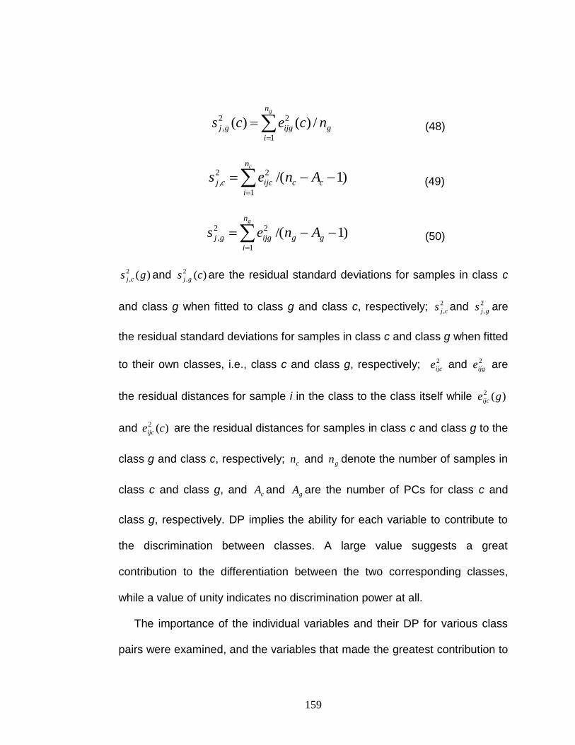
159
g
n
i
ijggj ncecsg
/)()(1
22
,
(48)
)1/(1
22
,
cc
n
i
ijccj Anesc
(49)
)1/(1
22
,
gg
n
i
ijggj Anesg
(50)
)(2
, gs cj and )(2
, cs gj are the residual standard deviations for samples in class c
and class g when fitted to class g and class c, respectively; 2
,cjs and 2
,gjs are
the residual standard deviations for samples in class c and class g when fitted
to their own classes, i.e., class c and class g, respectively; 2
ijce and 2
ijge are
the residual distances for sample i in the class to the class itself while )(2 geijc
and )(2 ceijc are the residual distances for samples in class c and class g to the
class g and class c, respectively; cn and gn denote the number of samples in
class c and class g, and cA and gA are the number of PCs for class c and
class g, respectively. DP implies the ability for each variable to contribute to
the discrimination between classes. A large value suggests a great
contribution to the differentiation between the two corresponding classes,
while a value of unity indicates no discrimination power at all.
The importance of the individual variables and their DP for various class
pairs were examined, and the variables that made the greatest contribution to

160
the class discrimination are listed in Table 25. When analyzing the
discriminating ability of the different variables, 2.08 ppm (DP = 8.29) was
found to be the chemical shift with the highest discriminating power, being
most effective in discriminating between the Heparin and DS classes.
Significant discriminating ability was also shown by 3.56 ppm (DP = 3.46),
4.46 ppm (DP = 3.05), 4.04 ppm (DP = 3.04) and 2.11 ppm (DP = 3.00). The
highest DP value in the Heparin vs OSCS, DS vs OSCS, Heparin vs [DS +
OSCS] and Heparin vs DS vs OSCS models was at 2.14 ppm, corresponding
to 61.88, 41.41, 38.63 and 34.86, respectively. The same chemical shift
contributed substantially to discriminating OSCS from all of the other classes.
Other variables showing a significant discriminating power were 4.07 ppm
(DP = 16.81), 2.20 ppm (DP = 15.19), 2.17 ppm (DP = 15.06), 5.01 ppm (DP
= 12.02) and 5.04 ppm (DP = 11.71) for Heparin vs OSCS; 2.17 ppm (DP =
15.64), 4.07 ppm (DP = 15.10), 3.80 ppm (DP = 13.95), 5.04 ppm (DP =
12.46), 3.95 ppm (DP = 12.34), 5.34 ppm (DP = 12.16) and 5.01 ppm (DP =
11.13) for Heparin vs [DS + OSCS]; and 4.31 ppm (DP = 12.80), 2.08 ppm
(DP = 12.32), 5.01 ppm (DP = 11.85) and 4.49 ppm (DP = 10.58) for DS vs
OSCS. For Heparin vs DS vs OSCS, the results in Table 25 show that the
variables with the greatest discriminating power are 2.14 ppm (DP = 34.86)
and 2.08 ppm (DP = 10.03), which are the characteristic chemical shifts of
OSCS and DS, respectively.

161
Table 25. Discriminant Powers (DP) of Variables (V) for Various Models
__________________________________________________________________________________
Order Hep vs DS Hep vs OSCS Hep vs [DS + OSCS] DS vs OSCS Hep vs DS vs OSCS
V (ppm) DP V (ppm) DP V (ppm) DP V (ppm) DP V (ppm) DP __________________________________________________________________________________
1 2.08 8.29 2.14 61.88 2.14 38.63 2.14 41.41 2.14 34.86
2 3.56 3.46 4.07 16.81 2.17 15.64 4.31 12.80 2.08 10.03
3 4.46 3.05 2.20 15.19 4.07 15.10 2.08 12.32 2.17 8.67
4 4.04 3.04 2.17 15.06 3.80 13.95 5.01 11.85 4.07 8.63
5 2.11 3.00 5.01 12.02 5.04 12.46 4.49 10.58 5.01 8.44
6 3.92 2.89 5.04 11.71 3.95 12.34 2.17 9.45 2.20 7.68
7 4.01 2.82 4.22 10.92 5.34 12.16 5.16 8.37 4.49 6.80
8 3.53 2.80 4.37 10.02 5.01 11.13 5.19 7.12 4.31 6.64
9 3.71 2.68 2.08 9.65 4.01 9.25 4.98 7.02 5.04 6.14
10 3.95 2.51 3.80 9.56 4.43 9.13 4.07 7.01 5.19 5.76
11 4.31 2.48 5.43 9.44 5.61 8.76 3.89 6.95 4.98 5.57
12 3.86 2.47 5.37 9.23 5.43 8.68 2.20 6.85 3.95 5.34
13 3.59 2.39 4.25 9.18 3.89 8.17 3.98 6.71 4.61 5.24
14 5.37 2.34 4.58 9.13 4.22 7.86 5.10 6.55 2.11 5.22
15 3.89 2.25 4.10 9.03 5.25 7.81 4.64 6.40 4.22 5.21
16 3.50 2.23 4.55 8.71 5.31 7.76 2.11 6.05 4.10 5.06
17 4.25 2.22 4.61 8.69 3.92 7.73 3.74 5.88 4.04 4.98
18 3.80 2.19 5.19 8.52 3.50 7.68 4.61 5.77 3.80 4.91
19 5.34 2.05 4.49 8.41 3.53 7.66 2.02 5.59 5.43 4.90
20 3.74 2.00 4.98 8.31 2.08 7.47 3.53 5.54 4.19 4.84
__________________________________________________________________________________
The SIMCA class distance is defined as the ratio of the sum of the residual
standard deviations for all variables within one class when fitted to the other
class to the sum of the residual standard deviations for all variables when
fitted to their own class [102]. The distance is used to measure how far two
models are from each other. The squared SIMCA class distance between
category c and category g is given by:

162
1
)(
))()((
),(2
,
2
,
1
2
,
2
,
12
gjcj
m
j
gjcj
m
j
ss
csgs
gcD (51)
When g = c, the first term is 1 and the distance between a category and itself
becomes 0. A class distance of less than 1 indicates that the two classes
overlap, while if a class distance is greater than 1 but smaller than 3, a partial
separation of the classes occurs. A model distance of greater than 3 indicates
separation of the classes. It was found that the SIMCA class distances were
4.9 for Heparin vs DS, 53.0 for Heparin vs OSCS, 35.2 for Heparin vs [DS +
OSCS], and 26.1 for DS vs OSCS. Therefore, DS was very close to Heparin
while OSCS was far from the Heparin, and not surprisingly, [DS + OSCS] was
intermediate between DS and OSCS.
4.3.1.2 Analysis of Heparin Samples Spiked with other GAGs
Heparin API can also contain GAGs other than DS, such as chondroitin
sulfate A (CSA) and heparan sulfate (HS). In addition, oversulfated version of
these GAGs other than CSA could be used to adulterate heparin in the future.
The methods described herein are expected to identify a wide range of
potential GAG-like contaminants in NMR data. To augment the usefulness of
the method, the blend samples of heparin spiked with non-, partially-, or fully
oversulfated CSA, DS and HS at the 1.0%, 5.0% and 10.0% weight percent
levels were tested for their class assignations from the built models, which

163
allowed us to investigate the capability of the models (e.g., Heparin, DS, and
OSCS) to accept or reject the blend samples, and hence to detect fraudulent
or contaminated products. The detailed compositions of the series of blends
as well as the test results from class modeling are summarized in Table 26.
As can be seen from Table 26, the blend samples were diverse when
compared to the Heparin, DS and OSCS classes. It covered multiple
components, including CSA, DS, heparan, crude and purified heparin with
varying degrees of sulfation and with component content ranging from 1% to
10%. The blend sample can be assigned to one or more classes if they are
situated within the statistical limits, and they can be considered to be outliers
if the distance is beyond the limits. Thus, a blend sample can be assigned to
a single class, more than one class, or none of the above defined classes.
Samples B28, B29 and B30 are blank ones, that is, they are pure heparin
samples. Therefore, it is not doubt that they are all accepted by the Heparin
class. In addition, the Heparin class accepts some samples with low content
(1%) of GAGs, such as B9 (1% HS), B18 (1% OS-HS), B21 (1% OS-Hep),
B24 (1% PS-CSA#1) and B27 (1% PS-CSA#2). The Heparin class rejects all
blend samples with high content of GAGs (5% and 10%) as well as four low
content samples, which are B3 (1% CSA), B6 (1% DS), B12 (1% FS-CSA)
and B15 (1% FS-DS).
Blends B4, B5 and B6 are heparin samples spiked with 10%, 5% and 1%
DS, respectively. As expected, they are all accepted by the DS class.

164
Table 26. The Compositions of the Series of Blends of Heparin Spiked with other
GAGs and Test Results from SIMCA Class Modeling
__________________________________________________________________________________
ID GAGs Content (%) Accepted (A) or Rejected (R) by the classes _________________________________________
Heparin DS OSCS __________________________________________________________________________________
B1 CSA 10 R R R
B2 CSA 5 R R R
B3 CSA 1 R R R
B4 DS 10 R A R
B5 DS 5 R A R
B6 DS 1 R A R
B7 HS 10 R R R
B8 HS 5 R R R
B9 HS 1 A A R
B10 FS-CSA 10 R R A
B11 FS-CSA 5 R R A
B12 FS-CSA 1 R R A
B13 FS-DS 10 R R R
B14 FS-DS 5 R R R
B15 FS-DS 1 R A R
B16 OS-HS 10 R R R
B17 OS-HS 5 R R R
B18 OS-HS 1 A A R
B19 OS-HEP 10 R R R
B20 OS-HEP 5 R R R
B21 OS-HEP 1 A R R
B22 PS-CSA#1 10 R R A
B23 PS-CSA#1 5 R R R
B24 PS-CSA#1 1 A R R
B25 PS-CSA#2 10 R R A
B26 PS-CSA#2 5 R R R
B27 PS-CSA#2 1 A R R
B28 Blank - A R R
B29 Blank - A R R
B30 Blank - A R R
__________________________________________________________________________________
CSA: Chondroitin Sulfate A; DS: Dermatan Sulfate ; HS: Heparan Sulfate; FS: Fully Sulfated;
OS: Over Sulfated; PS: Partially Sulfated; Blank: control (pure heparin sample).

165
Samples B13, B14 and B15 correspond to fully-sulfated DS with content of
10%, 5% and 1%, respectively. The DS class only accepts the low content of
sample (B15), and rejects B13 and B14. As with the Heparin class, samples
B9 (1% HS) and B18 (1%OS-HS) are also accepted into the DS class.
The OSCS class model accepts five blend samples, viz., B10, B11, B12,
B22, and B25. B10, B11 and B12 are heparin samples spiked with 10%, 5%
and 1% fully-sulfated CSA, i.e., OSCS, and hence they absolutely belong to
the OSCS class. Samples B22 and B25 contain 10% partially-sulfated CSA
and they present very similar structure to OSCS.
4.3.2 UNEQ Analysis
The heparin 1H NMR data set was also analyzed using the unequal class
modeling (UNEQ) method. UNEQ, similar to quadratic discriminant analysis
(QDA), is based on the assumption of multivariate normal distribution of the
measured or transformed variables for each class population. In general,
UNEQ represents each class by means of its centroid. In a specific class, the
category space or the distance of each sample from the barycenter (center of
mass) or centroid is calculated according to various measures that follow a
chi-squared distribution.
4.3.2.1 Stepwise LDA Variable Reduction
For UNEQ modeling, the data matrix of variances-covariances needs to be
inverted, which would be impossible if the number of samples is less than that

166
of the variables [79, 93]. Therefore, a preliminary variable reduction step is
necessary so that the data matrix for each category presents a high ratio
between the number of training samples and the number of variables. In
general, the number of samples is required to be at least three times greater
than that of variables. In order to select a subset of original variables that
affords the maximum improvement of the discriminating ability between
categories, stepwise linear discriminant analysis (SLDA) was performed
before UNEQ modeling.
In the present study, all variables entering the model had a threshold F-to-
enter value equal to or greater than the entry value, 1.0. If the number of
variables with F-to-enter ≥ 1.0 exceeds 1/3 (one third) of the samples, then
the number of variables retained in the model was taken as 1/3 of the sample
number. Preliminary variable reduction using stepwise LDA led to the
selection of 15, 14, 14 and 15 variables for Heparin vs DS, Heparin vs OSCS,
Heparin vs [DS + OSCS], and DS vs OSCS, respectively (Table 27). For
Heparin vs DS, chemical shift 2.08 ppm had the highest F-value (101.6), so it
was the most important variable for the differentiation of Heparin from DS.
The next most important variable was 3.53 ppm with F-value of 8.9. These
two variables (2.08 and 3.53 ppm) were also found to be highly discriminating
in SIMCA modeling. The variable 4.49 ppm was significant for Heparin vs
OSCS, Heparin vs [DS + OSCS] and DS vs OSCS with F-values of 14.0, 23.3
and 103.0, respectively. In addition, the variable 2.08 ppm was also important
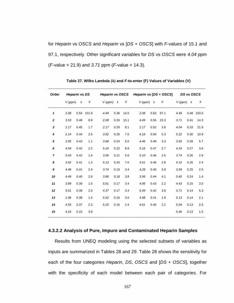
167
for Heparin vs OSCS and Heparin vs [DS + OSCS] with F-values of 15.1 and
97.1, respectively. Other significant variables for DS vs OSCS were 4.04 ppm
(F-value = 21.9) and 3.71 ppm (F-value = 14.3).
Table 27. Wilks Lambda (λ) and F-to-enter (F) Values of Variables (V)
__________________________________________________________________________________
Order Heparin vs DS Heparin vs OSCS Heparin vs [DS + OSCS] DS vs OSCS
V (ppm) λ F V (ppm) λ F V (ppm) λ F V (ppm) λ F
__________________________________________________________________________________
1 2.08 0.54 101.6 4.49 0.36 14.0 2.08 0.63 97.1 4.49 0.48 103.0
2 3.53 0.48 8.9 2.08 0.33 15.1 4.49 0.55 23.3 3.71 0.41 14.3
3 2.17 0.45 1.7 2.17 0.29 8.1 2.17 0.52 3.6 4.04 0.33 21.9
4 2.14 0.44 2.5 3.92 0.26 7.6 4.16 0.50 5.3 5.22 0.30 10.9
5 3.95 0.43 1.1 3.68 0.24 5.0 4.46 0.49 3.3 3.65 0.28 5.7
6 4.04 0.42 2.2 5.16 0.22 8.9 5.16 0.47 2.7 4.19 0.27 3.6
7 5.43 0.42 1.6 3.56 0.21 5.6 5.10 0.46 2.6 3.74 0.26 2.9
8 3.92 0.41 1.3 5.13 0.20 7.0 5.61 0.46 2.8 4.10 0.25 2.4
9 4.46 0.41 2.4 3.74 0.19 3.4 4.28 0.45 3.9 3.59 0.25 2.5
10 4.49 0.40 2.6 3.86 0.18 3.8 3.56 0.44 4.1 5.40 0.24 1.4
11 3.89 0.39 1.5 5.61 0.17 3.4 4.95 0.43 2.2 4.43 0.15 3.0
12 5.61 0.39 2.0 4.37 0.17 3.4 5.49 0.42 3.8 3.71 0.14 5.3
13 1.96 0.38 1.5 5.52 0.16 3.6 4.98 0.41 1.9 5.13 0.14 2.1
14 4.55 0.37 2.3 5.25 0.16 2.4 4.61 0.40 2.2 5.04 0.13 2.5
15 4.16 0.15 3.9 5.46 0.13 1.5
__________________________________________________________________________________
4.3.2.2 Analysis of Pure, Impure and Contaminated Heparin Samples
Results from UNEQ modeling using the selected subsets of variables as
inputs are summarized in Tables 28 and 29. Table 28 shows the sensitivity for
each of the four categories Heparin, DS, OSCS and [DS + OSCS], together
with the specificity of each model between each pair of categories. For

168
different systems, the subsets of selected variables were different, so that the
values of sensitivity and specificity varied within a certain range. The values
of sensitivity for Heparin, DS and OSCS were 84.7-87.5% (61-63/72), 80.0-
90.0% (40-45/50) and 87.0-91.3% (40-42/46), respectively. In all cases, the
sensitivity obtained using UNEQ was better than that evaluated with SIMCA
for which the values for Heparin, DS, OSCS and [DS + OSCS] were 77.8%
(56/72), 74.0% (37/50), 84.8% (39/46) and 79.2% (76/96), respectively.
Compared with SIMCA, UNEQ accepted 7 more Heparin, 8 more DS, 3 more
OSCS, and 5 more [DS + OSCS] samples by their specific category models
under optimal conditions. In the modeling of the category Heparin, 63 of the
72 samples were accepted by the category model built using UNEQ for
Heparin vs DS, while 56 of them were accepted by the SIMCA class model.
The differences between the two methods were far more marked when the
modeling of the other classes was considered. Of the 50 DS samples, 45
were correctly accepted by the UNEQ class model compared with 37 by the
SIMCA model. In addition, 42 out of the 46 OSCS samples and 81 out of the
96 [DS + OSCS] samples were correctly recognized by the UNEQ class
models compared with 39 out of 46 OSCS samples and 76 out of 96 [DS +
OSCS] samples by the SIMCA models.
Even though the sensitivity was greatly improved for the UNEQ model, a
corresponding decrease was observed in the specificity of UNEQ compared
to SIMCA. This is most evident by comparing the models for the Heparin and

169
DS classes as reported in Table 28. The specificity of the individual class
models was rather poor, most of the values being lower than 50%. The
classes DS and [DS + OSCS] accepted a large number of Heparin samples
(52/72 and 57/72, respectively), leading to significantly lower specificities
(27.8% and 20.8%) than the corresponding SIMCA values 81.9% (59/72) and
55.6% (40/72). The specificity of Heparin with respect to DS remarkably
decreased to 72.0% (36/50) from 90.0% (45/50), and that of Heparin to [DS +
OSCS] decreased to 82.3% (79/96) from 94.8% (91/96). Furthermore, the
UNEQ model showed a much poorer specificity for OSCS to Heparin and DS.
Table 28. Sensitivity and Specificity from UNEQ Class Modeling __________________________________________________________________________________
Model Sensitivity (%) Specificity (%) __________________________________________________________________________________
Heparin vs DS Heparin 87.5 (63/72) 72.0 (36/50) for DS
DS 80.0 (40/50) 27.8 (20/72) for Heparin
Heparin vs OSCS Heparin 84.7 (61/72) 100 (46/46) for OSCS
OSCS 87.0 (40/46) 26.4 (19/72) for Heparin
Heparin vs [DS + OSCS] Heparin 86.1 (62/72) 82.3 (79/96) for [DS + OSCS]
[DS + OSCS] 84.4 (81/96) 20.8 (15/72) for Heparin
DS vs OSCS DS 90.0 (45/50) 97.8 (45/46) for OSCS
OSCS 91.3 (42/46) 26.0 (13/50) for DS
Heparin vs DS vs OSCS Heparin 84.7 (61/72) 54.0 (27/50) for DS;
100 (46/46) for OSCS
DS 86.0 (43/50) 23.6 (17/72) for Heparin;
89.1 (41/46) for OSCS
OSCS 87.0 (40/46) 15.3 (11/72) for Heparin;
14.0 (7/50) for DS __________________________________________________________________________________

170
The values of the specificity for OSCS with respect to Heparin and DS
samples considerably decreased to 26.4% (19/72) and 26.0% (13/50) in
UNEQ compared with 100% (72/72) and 98.0% (49/50) in SIMCA. A major
exception was that of Heparin for OSCS, which remained perfect 100%
(46/46). The specificity of DS for OSCS was also high at 97.8% (45/46) for
UNEQ compared with 100% (46/46) for SIMCA.
The UNEQ class modeling results can be graphically visualized on the
Coomans plots as displayed in Figure 30. Compared with those correspon
ding to the SIMCA models, the Cooman‟s plots produced from the UNEQ
models revealed a large number of samples occupying the lower left quadrant
belonging to both classes. This outcome is a consequence of the low
specificity of the UNEQ class models.
Table 29 summarizes the results of the classification matrix evaluated by
means of leave-one-out cross-validation. Compared with SIMCA, the UNEQ
models exhibited better overall prediction ability. For example, the prediction
rates increased from 79.8% to 86.9% for Heparin vs [DS + OSCS] and from
75.6% to 84.5% for Heparin vs DS vs OSCS. Comparing these overall
abilities with those computed for the individual categories, it was noted that
the increase in the overall performance was mainly due to Heparin, and to a
lesser extent to DS, as the number of misclassified samples from these
classes was lower than in the corresponding SIMCA model. For Heparin vs
OSCS, Heparin vs [DS + OSCS] and Heparin vs DS vs OSCS, the prediction

171
A B
C D
Figure 30. Coomans plots for UNEQ class modeling. (A) Heparin vs OSCS; (B) Heparin vs DS; (C) Heparin vs [DS + OSCS]; (D) DS vs OSCS.
rates of the Heparin class increased from 87.5%, 65.3% and 62.5% for
SIMCA to 91.7%, 88.9% and 80.3% for UNEQ. For Heparin vs DS, DS vs
OSCS and Heparin vs DS vs OSCS, the prediction rates of DS class

172
increased from 84.0%, 78.0% and 72.0% in SIMCA to 86.0%, 88.0% and
78.0% in UNEQ.
Table 29. Classification Matrices from UNEQ Class Modeling
__________________________________________________________________________________
Model Training Prediction
__________________________________________________________________________________
Heparin vs DS Heparin DS Rate (%) Heparin DS Rate (%) Heparin 64 8 88.9 56 15 79.2
DS 3 47 94.0 7 43 86.0
Total - - 91.0 - - 81.8
Heparin vs OSCS Heparin OSCS Rate (%) Heparin OSCS Rate (%) Heparin 72 0 100 66 6 91.7
OSCS 0 46 100 1 45 97.8
Total - - 100 - - 94.9
Heparin vs [DS + OSCS] Heparin [DS + OSCS] Rate (%) Heparin [DS + OSCS] Rate (%) Heparin 72 0 100 64 8 88.9
[DS + OSCS] 14 82 85.4 14 82 85.4
Total - - 91.7 - - 86.9
DS vs OSCS DS OSCS Rate (%) DS OSCS Rate (%) DS 50 0 100 44 6 88.0
OSCS 0 46 100 2 44 95.7
Total - - 100 - - 91.7
Heparin vs DS vs OSCS Heparin DS OSCS Rate (%) Heparin DS OSCS Rate (%) Heparin 64 8 0 88.9 57 12 2 80.3
DS 4 46 0 92.0 8 39 3 78.0
OSCS 0 0 46 100 1 0 45 97.8
Total - - - 92.9 - - - 84.5
__________________________________________________________________________________

173
Chapter V
SUMMARY AND CONCLUSIONS
In order to differentiate heparin samples with varying amount of dermatan
sulfate (DS) impurities and oversulfated chondroitin sulfate (OSCS)
contaminants, proton NMR spectral data for heparin sodium active
pharmaceutical ingredient (API) samples from different manufacturers were
analyzed by multivariate chemometric methods for qualitative and quantitative
evaluation. The following conclusions were drawn based on multivariate
regression and pattern recognition separately.
5.1 Multivariate Regression for Predicting %Gal
In this study, the content of galactosamine (%Gal) in heparin (primarily
originating from the impurity dermatan sulfate, DS) was predicted from 1H
NMR spectral data by means of four multivariate analysis approaches, i.e.,
multiple linear regression (MLR), Ridge regression (RR), partial least squares
regression (PLSR), and support vector regression (SVR). Variable selection
was performed by genetic algorithms (GAs) or stepwise method in order to
build robust and reliable models. The results demonstrated that excellent
prediction performance was achieved in the determination of %Gal by all four
regression models under optimal conditions. Variable selection enhanced the
predictive ability substantially of all models, particularly the MLR model.

174
Simple models were obtained using a subset of selected variables that
predicted %Gal with high coefficients of determination and low prediction
errors.
In general, GA was superior to the stepwise method for variable selection.
Because GA can select any number of variables, a series of variables from 5
to 40 was selected to build predictive models. Over-fitted models based on
the training sets due to use of excessive variables led to poor predictive ability
on the test sets. Likewise, under-fitted models resulting from an insufficient
number of variables for model building led to statistically unstable models.
The optimal subsets for Datasets A and B were 10 and 30 variables,
respectively. After variable selection, the four regression models considered
in this study produced very similar results.
The range of %Gal in the samples influences many factors, i.e., the
selection of regression approach; the choice of variable selection method and
number of variables; and the interpretation of the models. Dataset A covered
the full range 0-10%Gal, while Dataset B was the subset covering 0-2%Gal.
As expected, Model A performed best for Dataset A while Model B was
preferred for Dataset B, indicating that a multi-stage modeling approach could
provide the best accuracy and range. Variable selection influenced the PLSR
and SVR models only slightly for Dataset A but was required to achieve
optimal results for Dataset B. All four MVR approaches (MLR, RR, PLSR, and
SVR) performed equally well and were robust under optimal conditions.

175
However, SVR was slightly superior to the other three regression approaches
when building models with Dataset B.
The present study offers assistance in selecting the appropriate MVR
approach to predict the %Gal in heparin based on analysis of 1D 1H-NMR
data. The results demonstrate that the combination of 1H NMR spectroscopy
and chemometric techniques provides a rapid and efficient way to
quantitatively determine the galactosamine content in heparin. More
generally, the present study underscores the importance in choosing the
appropriate regression method, variable selection approach, and fitting
parameters to build highly predictive regression models.
5.2 Classification for Pure, Impure and Contaminated Heparin Samples
To develop robust classification models for rapid screening of heparin
samples with varying amounts of dermatan sulfate (DS) impurities and
oversulfated chondroitin sulfate (OSCS) contaminants, several multivariate
statistical approaches, i.e., PCA, PLS-DA, LDA, kNN, CART, ANN and SVM,
were employed in combination with 1H NMR spectroscopy, and their
performance was compared using three data sets based on different chemical
shift regions (1.95-2.20, 3.10-5.70 and 1.95-5.70 ppm). It is shown that these
chemometric methods are useful tools for the exploration and visualization of
heparin NMR spectral data, and for the generation of classification models
with outstanding performance attributes. The large number of original
variables was reduced by chemometric methods into a much smaller number
176
of new variables (PCs, or latent variables) for effective clustering and
classification. The degree of success of the classification models in
discriminating the samples of pure heparin from those containing the impurity
DS and the contaminant OSCS depended on the specific chemometric
procedures for choosing the appropriate variables.
The well-known unsupervised chemometric method of PCA was used to
explore the similarities and differences in the complex pattern of overlapping
1H NMR signals found in the heparin spectra. The PCA results showed that
the samples were separated into two distinct clusters for the Heparin vs
OSCS groups, but the distinction between Heparin and DS was less evident.
Excellent discrimination of the Heparin samples from those samples
containing impurities (DS) and contaminants (OSCS) was achieved with the
supervised method PLS-DA.
The predictive performance of the models obtained from PLS-DA and LDA
were outstanding in differentiating Heparin from DS and OSCS with very few
misclassifications. In all cases, better classification rates (fewer
misclassifications) were attained for Heparin vs OSCS models than for
Heparin vs DS models regardless of the clustering and classification
approach. Under optimal conditions, success rates of 100% were frequently
achieved for discrimination between Heparin and OSCS samples. This
outcome is plausible, in view of the much closer similarity in the 1H NMR
spectral patterns between Heparin and DS than between Heparin and OSCS.

177
CART is a simple but powerful technique for class discrimination. It is able
to select the most relevant explanatory variables from the dataset and derive
classification rules on the basis of the reduced set of variables, so the tree-
structured models are easy to interpret and understand. For heparin and its
derivatives, the characteristic N-acetyl methyl proton chemical shifts are
located in the 1.95-2.20 ppm region. Specifically 2.08 and 2.15 ppm, the
characteristic chemical shifts of DS and OSCS, were found to possess the
greatest discriminating power for Heparin vs DS and Heparin vs OSCS,
respectively. After excluding the N-acetyl region, it was observed that the
classification and prediction rates in the local region 3.10-5.70 ppm were
evidently poor due to the lack of distinguishable characteristic peaks, implying
that the 2.0-2.2 ppm region plays an important role in discriminating heparin
from its impurities and contaminants for CART. Therefore, the variables or
chemical shifts selected in the CART analysis were interpretable and the
resulting trees were chemically justified.
As a widely applied learning approach, ANN is able to model highly
complex relationships with non-linear trends. Nevertheless, ANN modeling is
prone to overfitting and suffers difficulties with generalization since there are a
large number of model parameters to be optimized. By introducing the weight
decay in our study, the overfitting effect was greatly alleviated. As can be
seen from the obtained results, while the predictive performance of ANN
178
models on the test set is comparable to that of CART models for 1.95-2.20
ppm, it was slightly superior to CART in the 3.10-5.70 ppm region.
SVM represents a recent statistical learning technique and can model
complex non-linear boundaries through using adapted kernel functions. The
problem of overfitting can be effectively solved and remarkable generalization
performance can be achieved due to the high mapping power of the kernel,
resulting in a more highly predictive model. SVM can deal with high-
dimensional data with relatively few samples in the training set, and as a
consequence, no prior step of variable reduction is required. The SVM
algorithm does not provide the best solution automatically; model learning
requires optimization of the kernel parameter γ and the regularization
parameter C. The parameter tuning is a critical step, and the optimal values
are classically acquired by exhaustive search. In the present study, it was
quite easy to tune these parameters for Heparin vs OSCS, but for Heparin vs
DS, it needs to be very careful because it is difficult to discriminate Heparin
and DS owing to the similarity of samples on the 1.0% DS boundary. SVM
outperformed all other approaches for discrimination of the Heparin and DS
samples, and gave the best classification results in all cases (Figure 31). In
addition, it was found that the predictive rates for both 1.95-2.20 and 3.10-
5.70 ppm were very close to each other, indicating even minute structural
difference between heparin and DS can lead to remarkable discrimination
from SVM.

179
Heparin vs DS Heparin vs OSCS
Heparin vs [DS + OSCS] Heparin vs DS vs OSCS
Figure 31. Comparison of the classification performance of the six approaches.
The validated Heparin vs DS vs OSCS model was challenged for
classification of the blend samples in which the heparin APIs were spiked with
native or partially/fully oversulfated chondroitin sulfate A (CSA), dermatan

180
sulfate (DS) and heparan sulfate (HS) at the 1.0, 5.0, or 10.0 weight percent
levels. Overall, the results obtained from classification assignation on the
blends were excellent although the three multivariate pattern recognition
approaches are not class modeling techniques, which means that any object,
even a clear outlier, could be assigned to one class. We conclude that all of
the samples containing partially or fully oversulfated components, and the
potential GAG impurities, were readily distinguished from USP grade heparin
by the resulting models.
In summary, the present study reveals that 1H NMR spectroscopy, in
combination with multivariate chemometric methods, represent an effective
strategy for fast and reliable identification of impurities (DS) and contaminants
(OSCS) in heparin API samples. The pattern recognition approach applied
here may be useful in monitoring purity of other complex naturally derived
compounds.
5.3 Class Modeling Using SIMCA and UNEQ
In this work, two chemometric class-modeling techniques SIMCA and
UNEQ were employed to assess the quality of the heparin samples and to
perform pattern recognition among the various classes (pure heparin,
impurities and contaminants). Compared to pure classification techniques,
class-modeling approaches focus more on the analogies among the samples
from the same class than on the differences among the different classes;
hence, class modeling approaches allow us to explore the fundamental

181
details and individual characteristics of the classes. One of the advantages of
class modeling is that a sample can be recognized to be a member of one or
more classes, or none of the classes. The sensitivity, specificity and
prediction ability were computed as indicators of the quality of the models.
SIMCA can work on a small set of samples (as low as 10) per class and
does not apply any restriction on the number of measurement variables. This
is especially important because the number of variables is usually greater
than that of the analytical measurements (i.e. 1H NMR) of each sample. In
contrast, UNEQ requires variable reduction since the ratio of the number of
samples per class must be at least three-fold the number of variables in the
model. The computation of Wilks‟ lambda on the basis of stepwise linear
discriminant analysis (SLDA) enabled the selection of optimal subsets of
variables. The selected variables were useful for classification and
discrimination of the heparin samples by their origins. Depending on the
specific systems, the individual subsets of variables were different. The
subsets selected from two-class systems were more useful for discrimination
of the different classes.
For the heparin 1H NMR analytical data, significant differences were
observed between SIMCA and UNEQ analysis. The SIMCA models produced
excellent class separation between the Heparin and OSCS classes and
between the DS and OSCS classes, achieving nearly 100% specificity. On
the contrary, the UNEQ models produced excellent sensitivity but poor

182
specificity. Although the Heparin and DS classes rejected most of the OSCS
samples in UNEQ analysis, the OSCS class accepted a large number of
Heparin and DS samples, leading to extremely poor specificity. However,
when the computations were completed by UNEQ, the obtained models were
significantly better in terms of sensitivity and prediction ability. UNEQ
exhibited higher sensitivity with values of 88%, 90% and 91% for Heparin, DS
and OSCS compared to those of 78%, 74% and 85% from SIMCA.
The composition of the blend samples, in which the heparin APIs were
spiked with non-, partially-, or fully oversulfated chondroitin sulfate A (CSA),
dermatan sulfate (DS) and heparan sulfate (HS) at the 1.0%, 5.0% and 10.0%
weight percent levels, were highly diverse. These blend samples were
employed to challenge the Heparin, DS and OSCS class models. Overall, the
results obtained from SIMCA on the blends were excellent. The Heparin class
accepted pure heparin samples as well as some blends with low content (1%)
of GAGs, while the DS and OSCS classes accepted their respective GAG
blends. Importantly, some blends, such as OS-HS and OS-Hep, were
rejected by all the three class models. We conclude that all of the samples
containing partially or fully oversulfated components, and the potential GAG
impurities, were readily distinguished from USP grade heparin by the SIMCA
class models. The poor specificity (SPEC) of corresponding UNEQ class
models led to subpar performance metrics for the blend samples and,
therefore, were omitted here from detailed analysis.
183
According to USP specifications, the acceptance criterion for OSCS
content in heparin API and finished dose products is 0%. Although there are
no criteria for crude heparin products, it is desirable to use robust and
validated methods to identify and screen lots before they are fully processed.
The present study demonstrates that pattern recognition techniques, such as
SIMCA and UNEQ, are useful tools for discriminating pure and impure
heparin samples under investigation. The results reported here show that
through the employment of two chemometric class-modeling techniques,
namely SIMCA and UNEQ, it is possible to assess the quality of the samples.
In class modeling, it is important to consider the compromise between
sensitivity and specificity. Although it is significant to accept more samples
into their respective class models and achieve a higher sensitivity, these
models should not include too many samples from foreign classes, otherwise
the specificity will decline. It can be seen in the present study that the
specificities are higher for the SIMCA model while the sensitivities are greater
for the UNEQ model. The ability of UNEQ modeling to differentiate good
quality heparin from impure or contaminated samples was better than the
SIMCA modeling approach. However SIMCA modeling performed better in
distinguishing samples with high levels of DS from good quality heparin
compared to the UNEQ modeling.

184
Chapter VI
FUTURE DIRECTION FOR RESEARCH
Besides the proton NMR spectral data, the FDA also provided us with
strong-anion-exchange high-performance liquid chromatography (SAX-HPLC)
and near infrared (NIR) spectral data for a set of heparin samples obtained
from several foreign and domestic manufacturers.
During the heparin crisis, new tests and specifications were developed by
the US FDA and the USP in order to detect the contaminant as well as to
improve assurance of quality and purity of the drug product. In 2009, a new
USP monograph was put in place that included 1H NMR, a SAX-HPLC test,
and a percent galactosamine in total hexosamine measurement (% Gal),
which are assays orthogonal to each other [14, 15, 26, 58 ]. While the 1H
NMR spectra are primarily used to identify the presence or absence of
possible impurities or contaminants in heparin, SAX-HPLC data have
sufficiently resolved signals for the GAGs and have been used to quantify the
levels of DS or OSCS because the HPLC method is more sensitive and
robust for measurement of these GAGs in heparin. Figure 32 shows the
overlaid chromatograms of a heparin API spiked with CSB or OS-CSB at the
1.0%, 5.0% or 10.0% level. The CSB, heparin, and OS-CSB components
elute at 16.2, 20.4 and 22.5 min, respectively.
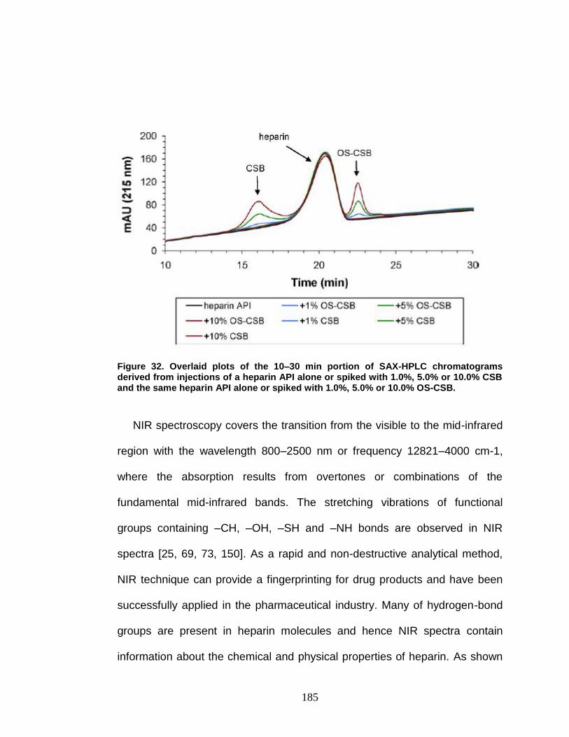
185
Figure 32. Overlaid plots of the 10–30 min portion of SAX-HPLC chromatograms derived from injections of a heparin API alone or spiked with 1.0%, 5.0% or 10.0% CSB and the same heparin API alone or spiked with 1.0%, 5.0% or 10.0% OS-CSB.
NIR spectroscopy covers the transition from the visible to the mid-infrared
region with the wavelength 800–2500 nm or frequency 12821–4000 cm-1,
where the absorption results from overtones or combinations of the
fundamental mid-infrared bands. The stretching vibrations of functional
groups containing –CH, –OH, –SH and –NH bonds are observed in NIR
spectra [25, 69, 73, 150]. As a rapid and non-destructive analytical method,
NIR technique can provide a fingerprinting for drug products and have been
successfully applied in the pharmaceutical industry. Many of hydrogen-bond
groups are present in heparin molecules and hence NIR spectra contain
information about the chemical and physical properties of heparin. As shown

186
in Figure 33, absorption bands at 5200 and 6900 cm-1 agree with Raman
spectrum studies. Heparin displays an irregular peak at 4730 cm-1 and a
shoulder at 6500 cm-1 which distinguish it from dermatan sulfate. OSCS has
two small peaks in the region around 4730 cm-1, another peak at 5800 cm-1
and a third peak at 7000 cm-1. The presence of OSCS as a contaminant in
heparin is expected to shift the large heparin peak at 6900 cm-1 to higher
energy.
Figure 33. Near infrared spectra of 108 heparin samples that contain DS impurities and OSCS contaminants.
In the future research, the use of 1H NMR, SAX-HPLC and NIR data in
combination with multivariate chemometric approaches is proposed to
conduct the following qualitative and quantitative analysis:

187
(1) Classification of samples for discriminating pure heparin, impurities
and contaminants according to the SAX-HPLC chromatographic data to
qualify raw materials and to control final products;
(2) Pattern recognition investigation for the three major components
heparin, DS and OSCS based on the NIR spectral data to demonstrate
the feasibility of NIR to identify contamination of heparin;
(3) Quantification of both DS and OSCS compositions in heparin sodium
by the specific signals in 1H NMR spectra coupled with multivariate
regression methods;
(4) Establishing calibration models by correlating NIR spectra of individual
heparin samples with the DS and OSCS content determined by SAX-
HPLC.

188
References
[1] Ampofo SA, Wang HM, Linhardt RJ. Disaccharide compositional analysis of heparin and heparan sulfate using capillary zone electrophoresis. Analytical Biochemistry. 1991, 199:249-255.
[2] Rabenstein DL. Heparin and heparan sulfate: structure and function.
Natural Product Report. 2002, 19:312-331.
[3] Casu B. Heparin structure. Haemostasis. 1990, 20:62-73.
[4] Sudo M, Sato K, Chaidedgumjorn A, Toyoda H, Toida T, Imanari T. 1H nuclear magnetic resonance spectroscopic analysis for determination of glucuronic and iduronic acids in dermatan sulfate, heparin, and heparan sulfate. Analytical Biochemistry. 2001, 297:42-51.
[5] Linhardt RJ. Hepairn: An important drug enters its seventh decade. Chemistry and Industry. 1991, 2:45-50.
[6] Lepor NE. Anticoagulation for acute coronary syndromes: from heparin to direct thrombin inhibitors. Reviews in Cardiovascular Medicine. 2007, 8 (suppl. 3):S9-S17.
[7] Fischer KG. Essentials of anticoagulation in hemodialysis. Hemodialysis International. 2007, 11:178-189.
[8] Maruyama T, Toida T, Imanari T, Yu G, Linhardt RJ. Conformational changes and anticoagulant activity of chondroitin sulfate following its O-sulfonation. Carbohydrate Research. 1998, 306:35-43.
[9] Guerrini M, Bisio A, Torri G. Combined quantitative 1H and 13C nuclear magnetic resonance spectroscopy for characterization of heparin preparations. Seminars in Thrombosis and Hemostasis. 2001, 27:473-482.
[10] Toida T, Maruyama T, Ogita Y, Suzuki A, Toyoda H, Imanari T, Linhardt RJ. Preparation and anticoagulant activity of fully O-sulphonated glycosaminoglycans. International Journal of Biological Macromolecules. 1999, 26:233-241.
[11] Griffin CC, Linhardt RJ, Van Gorp CL, Toida T, Hileman RE, Schubert RL, Brown SE. Isolation and characterization of heparan sulfate from crude porcine intestinal mucosal peptidoglycan heparin. Carbohydrate Research. 1995, 276:183-197.

189
[12] Pervin A, Gallo C, Jandik KA, Han XJ, Linhardt RJ. Preparation and
structural characterization of large heparin-derived oligosaccharides. Glycobiology. 1995, 5:83-95.
[13] Guerrini M, Zhang Z, Shriver Z, Naggi A, Masuko S, Langer R, Casu B,
Linhardt RJ, Torri G, Sasisekharan R. Orthogonal analytical approaches to detect potential contaminants in heparin. Proceedings of the National Academy of Sciences. 2009, 106(40):16956-16961.
[14] Keire DA, Trehy ML, Reepmeyer JC, Kolinski RE, Ye W, Dunn J,
Westenberger BJ, Buhse LF. Analysis of crude heparin by 1H NMR, capillary electrophoresis, and strong-anion-exchange-HPLC for contamination by over sulfated chondroitin sulfate. Journal of Pharmaceutical and Biomedical Analysis. 2010, 51:921-926.
[15] Keire DA, Mans DJ, Ye H, Kolinski RE, Buhse LF. Assay of possible economically motivated additives or native impurities levels in heparin by 1H NMR, SAX-HPLC, and anticoagulation time approaches. Journal of Pharmaceutical and Biomedical Analysis. 2010, 52:656-664.
[16] Zang Q, Keire DA, Wood RD, Buhse LF, Moore CMV, Nasr M, Al-Hakim A, Trehy ML, Welsh WJ. Determination of Galactosamine impurities in Heparin samples by multivariate regression analysis of their 1H NMR spectra. Analytical and Bioanalytical Chemistry. 2011, 399(2):635-649.
[17] Beyer T, Matz M, Brinz D, Rädler O, Wolf B, Norwig J, Abumann K,
Alban S, Holzgrabe U. Composition of OSCS-contaminated heparin occuring in 2008 in batches on the German market. European Journal of Pharmaceutical Sciences. 2010, 40:297-304.
[18] Korir AK, Larive CK. Advances in the separation, sensitive detection,
and characterization of heparin and heparan sulfate. Analytical and Bioanalytical Chemistry. 2009, 393:155-169.
[19] Casu B, Guerrini M, Naggi A, Torri G, De-Ambrosi L, Boveri G, Gonella
S, Cedro A, Ferró L, Lanzarotti E et al. Characterization of sulfation patterns of beef and pig mucosal heparins by nuclear magnetic resonance spectroscopy. Arzneimittelforschung. 1996, 46:472-477.
[20] Eldridge SL, Korir AK, Gutierrez SM, Campos F, Limtiaco JFK, Larive CK. Heterogeneity of depolymerized heparin SEC fractions: to pool or not to pool?. Carbohydrate Research. 2008, 343:2963-2970.
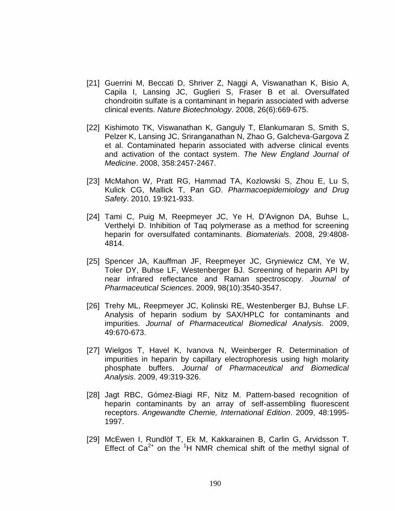
190
[21] Guerrini M, Beccati D, Shriver Z, Naggi A, Viswanathan K, Bisio A,
Capila I, Lansing JC, Guglieri S, Fraser B et al. Oversulfated chondroitin sulfate is a contaminant in heparin associated with adverse clinical events. Nature Biotechnology. 2008, 26(6):669-675.
[22] Kishimoto TK, Viswanathan K, Ganguly T, Elankumaran S, Smith S, Pelzer K, Lansing JC, Sriranganathan N, Zhao G, Galcheva-Gargova Z et al. Contaminated heparin associated with adverse clinical events and activation of the contact system. The New England Journal of Medicine. 2008, 358:2457-2467.
[23] McMahon W, Pratt RG, Hammad TA, Kozlowski S, Zhou E, Lu S,
Kulick CG, Mallick T, Pan GD. Pharmacoepidemiology and Drug Safety. 2010, 19:921-933.
[24] Tami C, Puig M, Reepmeyer JC, Ye H, D‟Avignon DA, Buhse L,
Verthelyi D. Inhibition of Taq polymerase as a method for screening heparin for oversulfated contaminants. Biomaterials. 2008, 29:4808-4814.
[25] Spencer JA, Kauffman JF, Reepmeyer JC, Gryniewicz CM, Ye W, Toler DY, Buhse LF, Westenberger BJ. Screening of heparin API by near infrared reflectance and Raman spectroscopy. Journal of Pharmaceutical Sciences. 2009, 98(10):3540-3547.
[26] Trehy ML, Reepmeyer JC, Kolinski RE, Westenberger BJ, Buhse LF. Analysis of heparin sodium by SAX/HPLC for contaminants and impurities. Journal of Pharmaceutical Biomedical Analysis. 2009, 49:670-673.
[27] Wielgos T, Havel K, Ivanova N, Weinberger R. Determination of impurities in heparin by capillary electrophoresis using high molarity phosphate buffers. Journal of Pharmaceutical and Biomedical Analysis. 2009, 49:319-326.
[28] Jagt RBC, Gómez-Biagi RF, Nitz M. Pattern-based recognition of heparin contaminants by an array of self-assembling fluorescent receptors. Angewandte Chemie, International Edition. 2009, 48:1995-1997.
[29] McEwen I, Rundlöf T, Ek M, Kakkarainen B, Carlin G, Arvidsson T. Effect of Ca2+ on the 1H NMR chemical shift of the methyl signal of

191
oversulphated chondroitin sulphate, a contaminant in heparin. Journal of Pharmaceutical and Biomedical Analysis. 2009, 49:816-819.
[30] Beyer T, Diehl B, Randel G, Humpfer E, Schäfer H, Spraul M, Schollmayer C, Holzgrabe U. Quality assessment of unfractionated heparin using 1H nuclear magnetic resonance spectroscopy. Journal of Pharmaceutical and Biomedical Analysis. 2008, 48:13-19.
[31] Zhang Z, Weïwer M, Li B, Kemp MM, Daman TH, Linhardt RJ. Oversulfated chondroitin sulfate: impact of a heparin impurity, associated with adverse clinical events, on low-molecular-weight heparin preparation. Journal of Medicinal Chemimstry. 2008, 51(18):5498-5501.
[32] Bigler P, Brenneisen R. Improved impurity fingerprinting of heparin by high resolution 1H NMR Spectroscopy. Journal of Pharmaceutical and Biomedical Analysis. 2009, 49:1060-1064.
[33] Sitkovwki J, Bednarek E, Bocian W, Kozerski L. Assessment of oversulfated chondroitin sulfate in low molecular weight and unfractioned heparins diffusion ordered nuclear magnetic resonance spectroscopy methods. Journal Medicinal Chemistry. 2008, 51:7663-7665.
[34] King JT, Desai UR. A capillary electrophoretic method for fingerprinting low molecular weight heparins. Analytical Biochemistry. 2008, 380:229-234.
[35] Domanig R, Jöbstl W, Gruber S, Freudemann T. One-dimensional cellulose acetate plate electrophoresis - A feasible method for analysis of dermatan sulfate and other glycosaminoglycan impurities in pharmaceutical heparin. Journal of Pharmaceutical and Biomedical Analysis. 2009, 49:151-155.
[36] Varmuza K, Filzmoser P. Introduction to Multivariate Statistical Analysis in Chemometrics. Boca Raton: CRC Press; 2009.
[37] Welsh WJ, Lin W, Tersigni SH, Collantes E, Duta R, Carey MS, Zielinski WL, Brower J, Spencer JA, Layloff TP. Pharmaceutical Fingerprinting: evaluation of neural networks and chemometric techniques for distinguishing among same-product manufacturers. Analytical Chemistry. 1996, 68(19):3473-3482.

192
[38] Tetko IV, Villa AEP, Aksenova TI, Zielinski WL, Brower J, Collantes ER, Welsh WJ. Application of a pruning algorithm to optimize artificial neural networks for pharmaceutical fingerprinting. Journal of Chemical Information and Computer Sciences. 1998, 38(4):660-668.
[39] Berrueta LA, Alonso-Salces RM, Héberger K. Supervised pattern
recognition in food analysis. Journal of Chromatography A. 2007, 1158:196-214.
[40] Rudd TR, Skidmore MA, Guimond SE, Cosentino C, Torri G, Fernig
DG, Lauder RM, Guerrini M, Yates EA. Glycosaminoglycan origin and structure revealed by multivariate analysis of NMR and CD spectra. Glycobiology. 2009, 19(1):52-67.
[41] Constantinou MA, Papakonstantinou E, Spraul M, Sevastiadou S, Costalos C, Koupparis MA, Shulpis K, Tsantili-Kakoulidou A, Mikros E. 1H NMR-based metabonomics for the diagnosis of inborn errors of metabolism in urine. Analytica Chimica Acta. 2005, 542:169-177.
[42] Keun HC, Ebbels TMD, Antti H, Bollard ME, Beckonert O, Holmes E,
Lindon JC, Nicholson JK. Improved analysis of multivariate data by variable stability scaling: application to NMR-based metabolic profiling. Analytica Chimica Acta. 2003, 490:265-276.
[43] Bailey NJC, Wang Y, Sampson J, Davis W, Whitcombe I, Hylands PJ,
Croft SL, Holmes E. Prediction of anti-plasmodial activity of Artemisia annua extracts: application of 1H NMR spectroscopy and chemometrics. Journal of Pharmaceutical and Biomedical Analysis. 2004, 35:117-126.
[44] Ruiz-Calero V, Saurina J, Galceran MT, Hernández-Cassou S,
Puignou L. Potentiality of proton nuclear magnetic resonance and multivariate calibration methods for the determination of dermatan sulfate contamination in heparin samples. Analyst. 2000, 125:933-938.
[45] Ruiz-Calero V, Saurina J, Hernández-Cassou S, Galceran MT, Puignou L. Proton nuclear magnetic resonance characterization of glycosaminolgycans using chemometric techniques. Analyst. 2002, 127:407-415.
[46] Ruiz-Calero V, Saurina J, Galceran MT, Hernández-Cassou S, Puignou L. Estimation of the composition of heparin mixtures from various origins using proton nuclear magnetic resonance and

193
multivariate calibration methods. Analytical and Bioanalytical Chemistry. 2002, 373:259-265.
[47] Holmes E, Antti H. Chemometric contributions to the evolution of
metabonomics: mathematical solutions to characterising and interpreting complex biological NMR spectra. Analyst. 2002:127, 1549-1557.
[48] Waters NJ, Holmes E, Waterfield CJ, Farrant RD, Nicholson JK. NMR
and pattern recognition studies on liver extracts and intact livers from rats treated with α-naphthylisothiocyanate. Biochemical Pharmacology. 2002, 64:67-77.
[49] Brereton RG. Chemometrics for pattern recognition. West Sussex: A
John Wiley and Sons, Ltd.; 2009.
[50] El-Abassy RM, Donfack P, Materny A. Visible Raman spectroscopy for the discrimination of olive oils from different vegetable oils and the detection of adulteration. Journal of Raman Spectroscopy. 2009, 40:1284-1289.
[51] Gurdeniz G, Ozen B. Detection of adulteration of extra-virgin olive oil
by chemometric analysis of mid-infrared spectral data. Food Chemistry. 2009, 116:519-525.
[52] Reid LM, O‟Donnell CP, Downey G. Potential of SPME-GC and
chemometrics to detect adulteration of soft fruit purées. Journal of Agricultural Food Chemistry. 2004, 52:421-427.
[53] de Veij M, Vandenabeele P, Hall KA, Fernandez FM, Green MD, White
NJ, Dondorp AM, Newton PN, Moens L. Fast detection and identification of counterfeit antimalarial tablets by Raman spectroscopy. Journal of Raman Spectroscopy. 2007, 38:181-187.
[54] de Veij M, Deneckere A, Vandenabeele P, de Kaste D, Moens L.
Detection of counterfeit Viagra with Raman spectroscopy. Journal of Pharmaceutical and Biomedical Analysis. 2008, 46:303-309.
[55] Storme-Paris I, Rebiere H, Matoga M, Civade C, Bonnet PA, Tissier
MH, Chaminade P. Challenging near infrared spectroscopy discriminating ability for counterfeit pharmaceuticals detection. Analytica Chimica Acta. 2010, 658:163-174.

194
[56] Zhang Z, Li B, Suwan J, Zhang F, Wang Z, Liu H, Mulloy B, Linhardt RJ. Analysis of pharmaceutical heparins and potential contaminants using 1H-NMR and PAGE. Journal of Pharmaceutical Sciences. 2009, 98(11):4017-4026.
[57] Rudd TR, Guimond SE, Skidmore MA, Duchesne L, Guerrini M, Torri
G, Cosentino C, Brown A, Clarke DT, Turnbull JE, Fernig DG, Yates EA. Influence of substitution pattern and cation binding on conformation and activity in heparin derivatives. Glycobiology. 2007, 17(9):983-993.
[58] Perlin AS, Sauriol F, Cooper B, Folkman J. Dermatan sulfate in
pharmaceutical heparins. Thrombbosis and Haemostasis. 1987, 58:792-793.
[59] Alban S, Lühn S, Schiemann S, Beyer T, Norwig J, Schilling C, Rädler
O, Wolf B, Matz M, Baumann K, Holzgrabe U. Comparison of established and novel purity tests for the quality control of heparin by means of a set of 177 heparin samples. Analytical and Bioanalytical Chemistry. 2011, 399(2):605-620.
[60] Keire DA, Ye H, Trehy ML, Ye W, Kolinski RE, Westenberger BJ,
Buhse LF, Nasr M, Al-Hakim A. Characterization of currently marketed heparin products: key tests for quality assurance. Analytical and Bioanalytical Chemistry. 2011, 399(2):581-591.
[61] Laurencin CT, Nair L. The FDA and safety – beyond the heparin crisis.
Nature Biotechnology. 2008, 26(6):621-623.
[62] Guerrini M, Shriver Z, Bisio A, Naggi A, Casu B, Sasisekharan R, Torri G. The tainted heparin story: an update. Thrombosis Haemostasis. 2009, 102:907-911.
[63] Beni S, Limtiaco JFK, Larive CK. Analysis and characterization of
heparin impurities. Analytical and Bioanalytical Chemistry. 2011, 399(2):527-539.
[64] Brustkern AM, Buhse LF, Nasr M, Al-Hakim A, Keire DA.
Characterization of currently marketed heparin products: reversed-phase ion-pairing liquid chromatography mass spectrometry of heparin digests. Analytical Chemistry. 2010, 82:9865-9870.

195
[65] Limtiaco JF, Jones CJ, Larive CK. Characterization of heparin impurities with HPLC-NMR using weak anion exchange chromatography. Analytical Chemistry. 2009, 81:10116-10123.
[66] Üstün B, Sanders KB, Dani P, Kellenbach ER. Quantification of
chondroitin sulfate and dermatan sulfate in danaparoid sodium by 1H NMR spectroscopy and PLS regression. Analytical and Bioanalytical Chemistry. 2011, 399:629-634.
[67] McEwen I, Mulloy B, Hellwig E, Kozerski L, Beyer T, Holzgrabe U,
Rodomonte A, Wanko R, Spieser JM. Determination of oversulphated chondroitin sulphate and dermatan sulphate in unfractioned heparin by 1H NMR. Pharmeuropa Bio/ the Biological Standardisation Programme. 2008, 1:31-39
[68] Mutihac L, Mutihac R. Mining in chemometrics. Analytica Chimica
Acta. 2008, 612:1-18.
[69] Roggo Y, Chalus P, Maurer L, Lema-Martinez C, Edmond A, Jent N. A review of near infrared spectroscopy and chemometrics in pharmaceutical technologies. Journal of Pharmaceutical and Biomedical Analysis. 2007, 44:683-700.
[70] Estienne F, Massart DL, Zanier-Szydlowski N, Marteau P. Multivariate
calibration with Raman spectroscopic data: a case study. Analytica Chimica Acta. 2000, 424:185-201.
[71] Leardi R. Genetic algorithms in chemometrics and chemistry: a review.
Journal of Chemometrics. 2001, 15:559-569.
[72] Jouan-Rimbaud D, Massart D, Leardi R, De Noord OE. Genetic algorithms as a tool for wavelength selection in multivariate calibration. Analytical Chemistry. 1995, 67:4295-4301.
[73] Liebmann B, Friedl A, Varmuza K. Determination of glucose and
ethanol in bioethanol production by near infrared spectroscopy and chemometrics. Analytica Chimica Acta. 2009, 642:171-178.
[74] Carneiro RL, Braga JWB, Bottoli CBG, Poppi RJ. Application of genetic
algorithm for selection of variables for the BLLS method applied to determination of pesticides and metabolites in wine. Analytica Chimica Acta. 2007, 595:51-58.

196
[75] Gourvénec S, Capron X, Massart DL. Genetic algorithms (GA) applied to the orthogonal projection approach (OPA) for variable selection. Analytica Chimica Acta. 2004, 519:11-21.
[76] Forshed J, Schuppe-Koistinen I, Jacobsson SP. Peak alignment of
NMR signals by means of a genetic algorithm. Analytica Chimica Acta. 2003, 487:189-199.
[77] Üstün B, Melssen WJ, Oudenhuijzen M, Buydens LMC. Determination
of optimal support vector regression parameters by genetic algorithms and simplex optimization. Analytica Chimica Acta. 2005, 544:292-305.
[78] Broadhurst D, Goodacre R, Jones A, Rowland JJ, Kell DB. Genetic
algorithms as a method for variable selection in multiple linear regression and partial least squares regression with applications to pyrolysis mass spectrometry. Analytica Chimica Acta. 1997, 348:71-86.
[79] Forina M, Oliveri P, Lanteri S, Casale M. Class-modeling techniques
classic and new for old and new problems. Chemometrics and Intelligent Laboratory Systems. 2008, 93:132-148.
[80] Marini F, Magri AL, Balestrieri F, Fabretti F, Marini D. Supervised
pattern recognition applied to the discrimination of the floral origin of six types of Italian honey samples. Analytica Chimica Acta. 2004, 515:117-125.
[81] Pérez-Magariño S, Ortega-Heras M, González-San José ML, Boger Z.
Comparative study of artificial neural network and multivariate methods to classify Spanish DO rose wines. Talanta. 2004, 62:983-990.
[82] Huang J, Brennan D, Sattler L, Alderman J, Lane B, O‟Mathuna C. A
comparison of calibration methods based on calibration data size and robustness. Chemometrics and Intelligent Laboratory Systems. 2002, 62:25-35.
[83] Czekaj T, Wu W, Walczak B. About kernel latent variable approaches
and SVM. Journal of Chemometrics. 2005, 19:341-354.
[84] Tistaert C, Dejaegher B, Nguyen Hoai N, Chataigné G, Riviere C, Nguyen Thi Hong V, Chau Van M, Quetin-Leclercq J, Vander Heyden Y. Potential antioxide compounds in Mallotus species fingerprints. Part I: Indication using linear multivariate calibration techniques. Analytica Chimica Acta. 2009, 649:24-32.

197
[85] Liu H, Zhang R, Yao X, Liu M, Hu Z, Fan B. Prediction of electrophoretic mobility of substituted aromatic acids in different aqueous-alcoholic solvents by capillary zone electrophoresis based on support vector machine. Analytica Chimica Acta. 2004, 525:31-41.
[86] Vapnik V. The nature of Statistical Learning Theory. New York:
Springer-Verlag; 1995.
[87] Vapnik V. Statistical Learning Theory. New York: John Wiley & Sons; 1998.
[88] Li H, Liang Y, Xu Q. Support vector machines and its applications in
chemistry. Chemometrics and Intelligent Laboratory Systems. 2009, 95:188-198.
[89] Thissen U, Pepers M, Üstün B, Melssen WJ, Buydens LMC.
Comparing support vector machines to PLS for spectral regression applications. Chemometrics and Intelligent Laboratory Systems. 2004, 73:169-179.
[90] Pan Y, Jiang J, Wang R, Cao H. Advantages of support vector
machine in QSPR studies for predicting auto-ignition temperatures of organic compounds. Chemometrics and Intelligent Laboratory Systems. 2008, 92:169-178.
[91] Collantes ER, Duta R, Welsh WJ, Zielinski WL, Brower J.
Preprocessing of HPLC trace impurity patterns by wavelet packets for pharmaceutical fingerprinting using artificial neural networks. Analytical Chemistry. 1997, 69(7):1392-1397.
[92] Zielinski WL, Brower JF, Welsh WJ, Collantes E, Layloff TP. A strategy
for developing consistent HPLC data for assessing sameness and difference in consistency of pharmaceutical products. American Pharmaceutical Review. 1998, 1:44-54.
[93] Marini F, Bucci R, Magrì AL, Magrì AD. Authentication of Italian CDO
wines by class-modeling techniques. Chemometrics and Intelligent Laboratory Systems. 2006, 84:164-171.
[94] Forina M, Oliveri P, Casale M, Lanteri S. Multivariate range modeling,
a new technique for multivariate class modeling: The uncertainty of the estimates of sensitivity and specificity. Analytica Chimica Acta. 2008, 622:85-93.

198
[95] Sáiz-Abajo MJ, González-Sáiz JM, Pizarro C. Near infrared spectroscopy and pattern recognition methods applied to the classification of vinegar according to raw material and elaboration process. Journal Near Infrared Spectroscopy. 2004, 12:207-219.
[96] Casale M, Armanino C, Casolino C, Forina M. Combining information
from headspace mass spectrometry and visible spectroscopy in the classification of the Ligurian olive oils. Analytica Chimica Acta. 2007, 589:89-95.
[97] Meléndez ME, Sánchez MS, Íñiguez M, Sarabia LA, Ortiz MC.
Psychophysical parameters of color and the chemometric characterization of wines of the certified denomination of origin „Rioja‟. Analytica Chimica Acta. 2001, 446:159-169.
[98] Sáiz-Abajo M, González-Sáiz J, Pizarro C. Classification of wine and
alcohol vinegar samples based on near-infrared spectroscopy, Feasibility study on the detection of adulterated vinegar samples. Journal of Agricultural and Food Chemistry. 2004, 52:7711-7719.
[99] Marinia F, Magria AL, Buccia R, Balestrierib F, Marini D. Class-
modeling techniques in the authentication of Italian oils from Sicily with a Protected Denomination of Origin (PDO). Chemometrics and Intelligent Laboratory Systems. 2006, 80:140-149.
[100] Nicholson JK, Connelly J, Lindon JC, Holmes E. Metabonomics: a
platform for studying drug toxicity and gene function. Nature Reviews Drug Discovery. 2002, 1:153-161.
[101] Ramadan Z, Jacobs D, Grigorov M, Kochhar S. Metabolic profiling
using principal component analysis, discriminant partial least squares, and genetic algorithms. Talanta. 2006, 68:1683-1691.
[102] Foot M, Mulholland M. Classification of chondroitin sulfate A,
chondroitin sulfate C, glucosamine hydrochloride and glucosamine 6 sulfate using chemometric techniques. Journal of Pharmaceutical and Biomedical Analysis. 2005, 38:397-407.
[103] Rezzi S, Axelson DE, Héberger K, Reniero F, Mariani C, Guillou C.
Classification of olive oils using high throughput flow 1H NMR fingerprinting with principal component analysis, linear discriminant analysis and probabilistic neural networks. Analytica Chimica Acta. 2005, 552:13-24.

199
[104] Kemsley EK. Discriminant analysis of high-dimensional data: a comparison of principal components analysis and partial least squares data reduction methods. Chemometrics and Intelligent Laboratory Systems. 1996, 33:47-61.
[105] Eriksson L, Antti H, Gottfries J, Holmes E, Johansson E, Lindgren F,
Long I, Lundstedt T, Trygg J, Wold S. Using chemometrics for navigating in the large data sets of genomics, proteomics, and metabonomics. Analytical and Bioanalytical Chemistry. 2004, 380:419-429.
[106] Whelehan OP, Earll ME, Johansson E, Toft M, Eriksson L. Detection of
ovarian cancer using chemometric analysis of proteomic profiles. Chemometrics and Intelligent Laboratory Systems. 2006, 84:82-87.
[107] Zhou J, Xu B, Huang J, Jia X, Xue J, Shi X, Xiao L, Li W. 1H-NMR-
based metabonomic and pattern recognition analysis for detection of oral squamous cell carcinoma. Clinica Chimica Acta. 2009, 401:8-13.
[108] Chevallier S, Bertrand D, Kohler A, Courcoux P. Application of PLS-DA
in multivariate image analysis. Journal of Chemometrics. 2006, 20:221-229.
[109] Ballabio D, Skov T, Leardi R, Bro R. Classification of GC-MS
measurements of wines by combining data dimension reduction and variable selection techniques. Journal of Chemometrics. 2008, 22:457-463.
[110] Pereira GE, Gaudillere JP, van Leeuwen C, Hilbert G, Maucourt M,
Deborde C, Moing A, Rolin D. 1H NMR metabolite fingerprints of grape berry: Comparison of vintage and soil effects in Bordeaux grapevine growing areas. Analytica Chimica Acta. 2006, 563:346-352.
[111] Domingo C, Arcis RW, Osorio E, Toledao M, Saurina J. Principal
component analysis and cluster analysis for the characterization of dental composites. Analyst. 2000, 125:2044-2048.
[112] Beckonert O, Bollard ME, Ebbels TMD, Keun HC, Antti H, Holmes E,
Lindon JC, Nicholson JK. NMR-based metabonomic toxicity classification: hierarchical cluster analysis and k-nearest-neighbor approaches. Analytica Chimica Acta. 2003, 490:3-15.

200
[113] Sikorska E, Gorecki T, Khmelinskii IV, Sikorski M, Koziol J. Classification of edible oils using synchronous scanning fluorescence spectroscopy. Food Chemistry. 2005, 89:217-225.
[114] Caetano S, Aires-de-Sousa J, Daszykowski M, Vander Heyden Y.
Prediction of enantioselectivity using chirality codes and classification and regression trees. Analytica Chimica Acta. 2005, 544:315-326.
[115] Questier F, Put R, Coomans D, Walczak B, Vander Heyden Y. The use
of CART and multivariate regression trees for supervised and unsupervised feature selection. Chemometrics and Intelligent Laboratory Systems. 2005, 76:45-54.
[116] Deconinck E, Hancock T, Coomans D, Massart DL, Vander Heyden Y.
Classification of drugs in absorption classes using the classification and regression trees (CART) methodology. Journal of Pharmaceutical and Biomedical Analysis. 2005, 39:91-103.
[117] Caetano S, Üstun B, Hennessy S, Smeyers-Verbeke J, Melssen W,
Downey G, Buydens L, Heyden YV. Geographical classification of olive oils by the application of CART and SVM to their FT-IR. Journal of Chemometrics. 2007, 21:324-334.
[118] Marini F. Artificial neural networks in foodstuff analyses: trends and
perspectives, a review. Analytica Chimica Acta. 2009, 635:121-131. [119] Agatonovic-Kustrin S, Beresford R. Basic concepts of artificial neural
network (ANN) modeling and its application in pharmaceutical research. Journal of Pharmaceutical and Biomedical Analysis. 2000, 22:717-727.
[120] Ginoris YP, Amaral AL, Nicolau A, Coelho MAZ, Ferreira EC.
Recognition of protozoa and metazoa using image analysis tools, discriminant analysis, neural networks and decision trees. Analytica Chimica Acta, 2007. 595:160-169.
[121] Hernández-Caraballo EA, Rivas F, Pérez AG, Marcó-Parra LM.
Evaluation of chemometric techniques and artificial neural networks for cancer screening using Cu, Fe, Se and Zn concentrations in blood serum. Analytica Chimica Acta. 2005, 533:161-168.
[122] Ma Q, Yan A, Hu Z, Li Z, Fan B. Principal component analysis and
artificial neural networks applied to the classification of Chinese pottery of neolithic age. Analytica Chimica Acta. 2000, 406:247-256.

201
[123] Belousov AI, Verzakov SA, von Frese J. Applicational aspects of aspects of support vector machines. Journal of Chemometrics. 2002, 16:482-489.
[124] Xu Y, Zomer S, Brereton RG. Support vector machines: a recent method for classification in chemometrics. Critical Review in Analytical Chemimstry. 2006, 36:177-188.
[125] Devos O, Ruckebusch C, Durand A, Duponchel L, Huvenne JP. Support vector machines (SVM) in near infrared (NIR) spectroscopy: focus on parameters optimization and model interpretation. Chemometrics and Intelligent Laboratory Systems. 2009, 96:27-33.
[126] Chen Q, Guo Z, Zhao J. Identification of green tea‟s (Camellia sinensis (L.)) quality level according to measurement of main catechins and caffeine contents by HPLC and support vector classification pattern recognition. Journal of Pharmaceutical and Biomedical Analysis. 2008, 48:1321-1325.
[127] Amendolia SR, Cossu G, Ganadu ML, Golosio B, Masala GL, Mura GM. A comparative study of k-nearest neighbour, support vector machine and multi-layer perceptron for thalassemia screening. Chemometrics and Intelligent Laboratory Systems. 2003, 69:13-20.
[128] Zomer Z, Guillo C, Brereton RG, Hanna-Brown M. Toxicological classification of urine samples using pattern recognition techniques and capillary electrophoresis. Analytical and Bioanalytical Chemistry. 2003, 378:2008-2020.
[129] Zheng L, Watson DG, Johnston BF, Clark RL, Edrada-Ebel R, Elseheri W. A chemometric study of chromatograms of tea extracts by correlation optimization warping in conjunction with PCA, support vector machines and random forest data modeling. Analytica Chimica Acta. 2009, 642:257-265.
[130] Fernández Piernz JA, Baeten V, Michotte Renier A, Cogdill RP, Dardenne P. Combination of support vector machines (SVM) and near-infrared (NIR) imaging spectroscopy for the detection of meat and bone meal (MBM) in compound feeds. Journal of Chemometrics. 2004, 18:341-349.
[131] Yao XJ, Panaye A, Doucet JP, Chen HF, Zhang RS, Fan BT, Liu MC, Hu ZD. Comparative classification study of toxicity mechanisms using support vector machines and radial basis function neural networks. Analytica Chimica Acta. 2005, 535:259-273.

202
[132] Ren Y, Liu H, Xue C, Yao X, Liu M, Fan B. Classification study of skin sensitizers based on support vector machine and linear discriminant analysis. Analytica Chimica Acta. 2006, 572:272-282.
[133] Zhang Q, Yoon S, Welsh WJ. Improved method for predicting β-turn
suing support vector machine. Bioinformatics. 2005, 21(10):2370-2374. [134] Zang Q, Keire DA, Wood RD, Buhse LF, Moore CMV, Nasr M, Al-
Hakim A, Trehy ML, Welsh WJ. Class modeling analysis of heparin 1H NMR spectral data using the soft independent modeling of class analogy and unequal class modeling techniques. Analytical Chemistry. 2011, 83(3):1030-1039.
[135] Parisi D, Magliulo M, Nanni P, Casale M, Forina M, Roda A. Analysis
and classification of bacteria by matrix-assisted laser desorption/ ionization time-of-flight mass spectrometry and a chemometric approach. Analytical and Bioanalytical Chemistry. 2008, 391:2127-2134.
[136] Candolfi A, De Maesschalck R, Massart DL, Hailey PA, Harrington
ACE. Identification of pharmaceutical excipients using NIR spectroscopy and SIMCA. Journal of Pharmaceutical and Biomedical Analysis. 1999, 19:923-935.
[137] Alonso-Salces RM, Herrero C, Barranco A, Berrueta LA, Gallo B,
Vicente F. Classification of apple fruits according to their maturity state by the pattern recognition analysis of their polyphenolic compositions. Food Chemistry. 2005, 93:113-123.
[138] Weljie AM, Newton J, Mercier P, Carison E, Slupsky CM. Targeted
profiling: quantitative analysis of 1H NMR metabolomics data. Analytical Chemistry. 2006, 78:4430-4442.
[139] R: software, a language and environment for statistical computing. R
Development Core Team, Foundation for Statistical Computing, www.r-project.org.
[140] Maindonald J, Braun J. Data analysis and graphics using R.
Cambridge (UK): Cambridge University Press; 2003. [141] Wehrens R. Chemometrics with R: multivariate data analysis in the
natural sciences and life sciences. Berlin Heidelberg: Springer-Verlag; 2011.
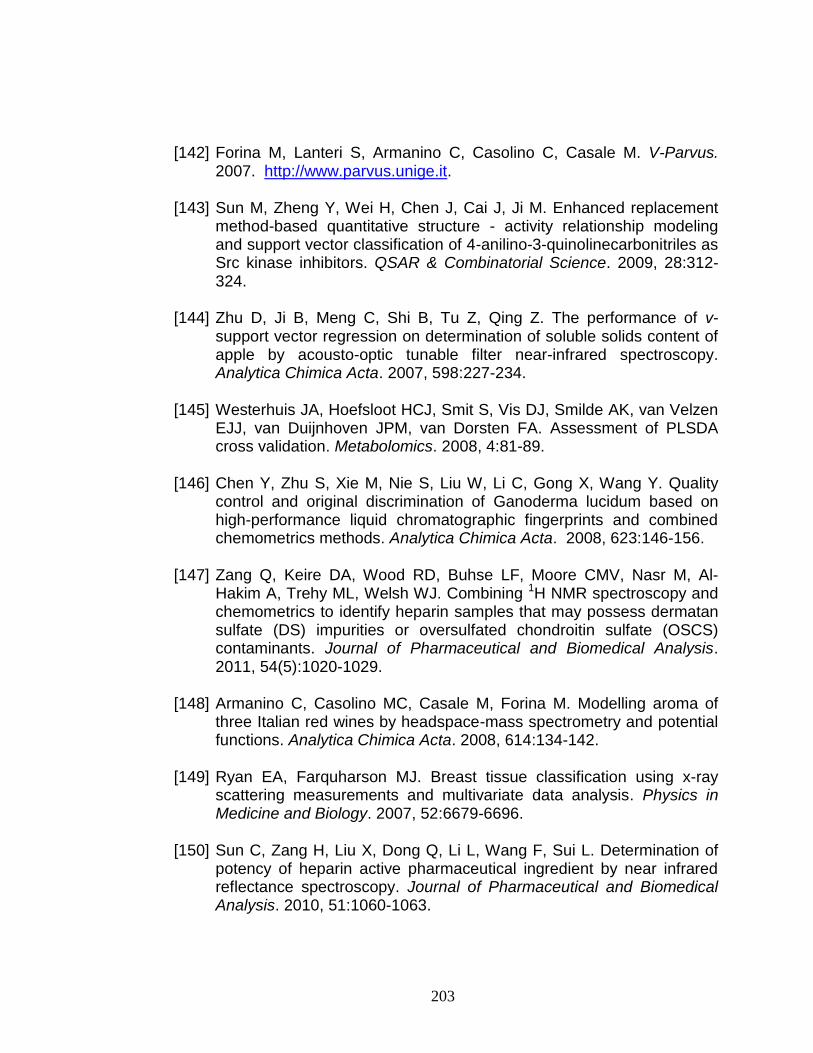
203
[142] Forina M, Lanteri S, Armanino C, Casolino C, Casale M. V-Parvus. 2007. http://www.parvus.unige.it.
[143] Sun M, Zheng Y, Wei H, Chen J, Cai J, Ji M. Enhanced replacement
method-based quantitative structure - activity relationship modeling and support vector classification of 4-anilino-3-quinolinecarbonitriles as Src kinase inhibitors. QSAR & Combinatorial Science. 2009, 28:312-324.
[144] Zhu D, Ji B, Meng C, Shi B, Tu Z, Qing Z. The performance of v-
support vector regression on determination of soluble solids content of apple by acousto-optic tunable filter near-infrared spectroscopy. Analytica Chimica Acta. 2007, 598:227-234.
[145] Westerhuis JA, Hoefsloot HCJ, Smit S, Vis DJ, Smilde AK, van Velzen
EJJ, van Duijnhoven JPM, van Dorsten FA. Assessment of PLSDA cross validation. Metabolomics. 2008, 4:81-89.
[146] Chen Y, Zhu S, Xie M, Nie S, Liu W, Li C, Gong X, Wang Y. Quality
control and original discrimination of Ganoderma lucidum based on high-performance liquid chromatographic fingerprints and combined chemometrics methods. Analytica Chimica Acta. 2008, 623:146-156.
[147] Zang Q, Keire DA, Wood RD, Buhse LF, Moore CMV, Nasr M, Al-
Hakim A, Trehy ML, Welsh WJ. Combining 1H NMR spectroscopy and chemometrics to identify heparin samples that may possess dermatan sulfate (DS) impurities or oversulfated chondroitin sulfate (OSCS) contaminants. Journal of Pharmaceutical and Biomedical Analysis. 2011, 54(5):1020-1029.
[148] Armanino C, Casolino MC, Casale M, Forina M. Modelling aroma of
three Italian red wines by headspace-mass spectrometry and potential functions. Analytica Chimica Acta. 2008, 614:134-142.
[149] Ryan EA, Farquharson MJ. Breast tissue classification using x-ray
scattering measurements and multivariate data analysis. Physics in Medicine and Biology. 2007, 52:6679-6696.
[150] Sun C, Zang H, Liu X, Dong Q, Li L, Wang F, Sui L. Determination of
potency of heparin active pharmaceutical ingredient by near infrared reflectance spectroscopy. Journal of Pharmaceutical and Biomedical Analysis. 2010, 51:1060-1063.

204
Appendix A: Abbreviations
ANN: artificial neural network APIs: active pharmaceutical ingredients BIC: Bayes information criterion CART: classification and regression tree CE: capillary electrophoresis CSA: chondroitin sulfate A CSB: chondroitin sulfate B CSC: chondroitin sulfate C CV: cross validation DP: discriminant power DPA: Division of Pharmaceutical Analysis DS: dermatan sulfate DSS: 4, 4-dimethyl-4-silapentane-1-sulfonic acid FDA: the US Food and Drug Administration GAG: glycosaminoglycan GAs: genetic algorithms GCV: generalized cross-validation HA: hyaluronic acid HCA: hierarchical cluster analysis HPLC: high-performance liquid chromatography HS: heparan sulfate

205
kNN: k-nearest neighbors
LDA: linear discriminant analysis LOO-CV: leave-one-out cross-validation MLR: multiple linear regression MSEP: mean squared error for prediction MVR: multivariate regression NIR: near infrared NMR: nuclear magnetic resonance OSCS: oversulfated chondroitin sulfate PC: principal component PCA: principal component analysis PE: processing element PLS-DA: partial least squares discriminant analysis PLSR: partial least squares regression PRESS: predictive error sum of squares QDA: quadratic discriminant analysis RBF: radial basis function RMSE: root mean squared error RR: Ridge regression RSD: relative standard deviation RSE: relative standard error RSS: residual sum of squares

206
SAX-HPLC: strong-anion-exchange high-performance liquid chromatography SEP: standard error of prediction SIMCA: soft-independent modeling of class analogy SLDA: stepwise linear discriminant analysis SVM: support vector machine SVR: support vector regression TNs: terminal nodes UNEQ: unequal dispersed classes USP: the United States Pharmacopeia

207
Appendix B: Index
Active pharmaceutical ingredients (APIs): 2, 5, 6, 9, 11, 21, 22, 32, 70, 72-75, 77, 78, 148, 165, 177, 183, 184, 186, 187, 189, 190 Allergic: 5, 25, 26 Anaphylactic reaction: 2, 25 Anticoagulant: 1, 4, 16, 17, 21-24, 27 Artificial neural network (ANN): 3, 13, 57-59, 80, 136-141, 144-147, 149, 151, 180, 182 Bayes information criterion (BIC): 84-87 Blend: 15, 75, 148-151, 165-168, 183, 186, 187 Calibration: 11, 33, 34, 39, 42, 68, 74, 80, 87, 88, 92, 192 Capillary electrophoresis (CE): 6, 7, 27, 31, 32, 70, 72, 111 Carbohydrate: 4, 16, 17, 28 Centroid: 66, 67, 169 Chemical shift: 13, 76, 78, 79, 131, 132, 135, 136, 145, 163, 170, 180-182 Chemometric: 2, 3, 7-12, 14-16, 33, 35, 41, 46, 48, 67, 70, 71, 73, 78- 80, 111, 177, 179, 180, 183, 185, 187, 191 Chi-squared distribution: 66, 169 Chondroitin sulfate: 1, 2, 4-6, 18, 19, 21, 22, 27, 30, 32, 70, 75, 148, 151, 165, 168, 183, 186 Class modeling: 14, 15, 47, 48, 63, 67, 80, 152, 155, 157, 160, 166, 168, 172, 173, 175, 176, 183, 185, 187 Classification: 3, 4, 9, 10, 12-15, 33, 43, 46, 47, 50, 51, 53-57, 60, 62, 72, 73, 80, 83, 111, 112, 117-120, 124-133, 135, 138, 140-142, 144-148, 151, 152, 158-161, 174, 175, 179-181, 183-185, 192

208
Classification and regression tree (CART): 3, 13, 54, 55, 131, 133, 135, 136, 141, 144-147, 149, 151, 180-182 Cluster: 13, 46, 49, 50, 112, 113, 148, 149, 156, 180 Clustering: 2, 12, 46, 117, 180, 181 Coefficient of determination: 12, 80, 102, 109, 178 Collinearity: 40, 98, 102, 103 Confidence level: 49, 64, 65, 67, 89, 152, 153, 155, 179 Contaminant: 2, 4-7, 9, 11, 13, 15, 16, 24-27, 29, 31, 67-69, 71, 75, 113, 117, 130, 136, 148, 152, 165, 177, 179-181, 183, 185, 189, 191, 192 Coomans plot: 155-158, 173, 176 Cost complexity parameter: 56, 134 Cost function: 43, 44, 108 Covariance: 37, 38, 42, 52, 66, 67, 122, 169 Cross entropy: 137 Cross validation (CV): 54, 57, 63, 99, 100, 104, 108, 123, 125, 128, 131, 134, 138, 141 Dendrogram: 148-150 Dermatan sulfate (DS): 1, 2, 4-7, 9, 10, 12-14, 15, 18, 19, 21, 22, 28-31, 67, 68, 70, 72-76, 78, 86, 89, 111, 113, 114, 116-121, 123-136, 138-140, 142-154, 156-161, 163-168, 170-177, 179-181, 183, 184, 186-189, 191, 192 Deviance: 137 Dimension: 7, 13, 18, 27, 42, 46, 48-50, 52, 53, 61, 63, 79, 103, 107, 111, 112, 118, 121, 122, 137, 182 Disaccharide: 4-6, 9, 17, 19, 20, 29, 30, 76 Discriminant power (DP): 161-164

209
Euclidean distance: 43, 53, 61, 64, 66, 149, 150 Feature space: 42, 45, 48, 61, 107 Fingerprint: 3, 9, 10, 11, 16, 28, 190 Galactosamine: 1, 5, 7, 11, 12, 18, 28, 29, 32, 72, 74, 76, 83, 189 Galactosamine content (%Gal): 1-3, 5, 7, 8, 11, 12, 15, 73-75, 81, 83, 87, 89, 92, 94-98, 105, 107, 109, 177-179 Gaussian: 46, 48, 63 Generalization: 61, 63, 108, 136, 182 Generalized cross-validation (GCV): 99, 100 Genetic algorithms (GAs): 3, 8, 12, 35, 36, 80, 83, 87-102, 104-107, 109, 110, 177, 178 Gini index: 55, 131 Glycosaminoglycan (GAG): 1, 4, 6, 11, 16-18, 20-22, 32, 75, 148-151, 165-168, 183, 187, 189 Grid search: 108, 141, 143 Heparan sulfate (HS): 4, 15, 19, 21, 22, 75, 148-151, 165-168, 183, 186, 187 Hexosamine: 17, 18, 32, 73, 189 Hexuronic acid: 17 Hidden layer: 58-60, 136-138 Hierarchical cluster analysis (HCA): 13, 46, 148, 149 High performance liquid chromatography (HPLC): 1, 6, 7, 11, 12, 27, 32, 74, 75, 81, 92, 94, 97, 119, 189-192 Hyaluronic acid (HA): 5, 21 Hyperplane: 60-62, 158,

210
Impure: 2, 3, 11, 72, 73, 78, 83, 111, 117, 136, 142, 152, 153, 171, 179, 187, 188 Impurity: 1, 2, 4-6, 9, 13, 21, 22, 30, 31, 46, 67, 73, 75, 111, 113, 117, 136, 146, 148, 150, 152, 177, 179-181, 183, 185, 187, 189, 191, 192 Inner product: 45 Input: 42, 50, 58-61, 78, 87, 107, 126, 136, 138, 144, 171 Kernel function: 42, 45, 46, 61-63, 92, 107-110, 141, 178, 182 k-nearest-neighbor (kNN): 3, 13, 53, 114, 126-130, 152, 180 Lagrange multiplier: 44, 107 Latent variable: 41, 42, 51, 103, 117, 180 Leave-one-out cross-validation (LOO-CV): 14, 42, 82, 103, 119, 124, 126, 127, 129, 158, 174 Linear discriminant analysis (LDA): 3, 13, 52, 53, 80, 114, 121-126, 129, 152, 181, 189 Loss function: 42, 43 Mahalanobis distance: 52, 66, 67, 121, 122 Mapping function: 45, 62, 182 Margin: 60-62, 108, 141 Mean squared error for prediction (MSEP): 99 Misclassification: 53, 55, 57, 62, 117-121, 124, 126, 128, 129, 133, 139, 142, 144-146, 154, 159, 181 Model parameter: 93, 98, 101, 106, 110, 133, 140, 144, 182 Multiple linear regression (MLR): 3, 8, 12, 39-41, 83, 86, 92, 93, 96, 98, 102, 103, 107, 177-179 Multivariate: 3, 7-15, 33, 34, 39, 41, 48-51, 67, 68, 72-74, 78, 80, 83, 87, 92, 103, 107, 111, 148, 161, 169, 177, 180, 183, 191, 192

211
Multivariate regression (MVR): 3, 12, 34, 39, 41, 72, 83, 92, 107, 177, 192 Near infrared (NIR): 70, 71, 189-192 Normal distribution: 39, 48, 66, 67, 169 Nuclear magnetic resonance (NMR): 1-3, 6-16, 27-29, 31, 32, 48, 49, 67, 68, 71, 72, 74-78, 83, 87, 92, 94, 96, 97, 100, 107, 111-113, 146, 152, 153, 159, 165, 169, 177, 179-181, 183, 185, 186, 189, 191, 192 Objective function: 62 One standard deviation: 129, 134 Optimization: 33-35, 44, 62, 87, 108, 141, 182 Output: 51, 54, 58-60, 89, 136, 137 Overfitting: 13, 53, 54, 62, 63, 92, 102, 108, 109, 124, 137, 138, 141, 178, 182 Oversulfated chondroitin sulfate (OSCS): 2, 6, 7, 9-16, 19, 25, 27, 28, 30-32, 67-73, 75-78, 111, 113, 115-136, 138-145, 147-161, 163-168, 170-177, 179-184, 186, 187, 189-192 Partial least squares discriminant analysis (PLS-DA): 3, 13, 50-53, 68, 80, 112, 114-121, 124, 126, 129, 152, 180, 181 Partial least squares regression (PLSR): 3, 8, 12, 41, 70, 71, 80, 83, 86, 103-107, 109, 177-179 Pattern recognition: 2, 7, 10, 11, 46, 47, 52, 57, 60, 72, 78, 111, 114, 121, 144, 177, 183, 184, 185, 187, 192 Polysaccharide: 4, 17, 20, 21 Predictive error sum of squares (PRESS): 103 Principal components (PC): 49, 50, 63, 64, 68, 69, 103, 105, 106, 112, 113, 118-121, 126, 128-130, 152-154, 158, 162, 180 Principal components analysis (PCA): 3, 13, 46, 48-51, 63, 68-70, 112, 114-117, 126, 128, 152, 180

212
Quadratic discriminant analysis (QDA): 48, 66, 169 Radial basis function (RBF): 45, 46, 62, 108, 109, 141 Regression coefficient: 39-44, 98-100, 102, 108 Regularization parameter: 41, 43, 62, 92, 108, 141, 182 Relative standard deviation (RSD): 80, 81, 93, 101, 102, 105, 106, 110 Relative standard error (RSE): 105 Residual standard deviation: 64, 161, 162, 164 Residual sum of squares (RSS): 40, 84 Ridge regression (RR): 3, 8, 12, 40, 41, 80, 83, 86, 92, 98-102, 177 Root mean squared error (RMSE): 80, 81, 93, 96, 101, 102, 105-107, 110 Screening: 2, 9, 15, 27, 31, 70-72, 111, 179 Sensitivity: 14, 27, 65, 154, 171-173, 185-187 Slack variable: 43, 62 Soft-independent modeling of class analogy (SIMCA): 3, 14, 15, 48, 63-65, 67, 152-154, 157-161, 164, 165, 171-174, 185-188 Specificity: 14, 65, 154, 158, 171-174, 185-187 Spectra: 2, 3, 6, 9-11, 16, 28, 29, 48, 49, 68, 70, 71, 75-79, 112, 113, 142, 152, 159, 180, 189-191 Spectral data: 39, 69, 72, 74, 83, 112, 177, 180, 189, 192 Standard error of prediction (SEP): 103-105 Stepwise linear discriminant analysis (SLDA): 14, 37, 122, 169, 185 Stepwise selection: 12, 83, 95, 96 Strong anion exchange (SAX): 6, 7, 11, 32, 119, 189-192
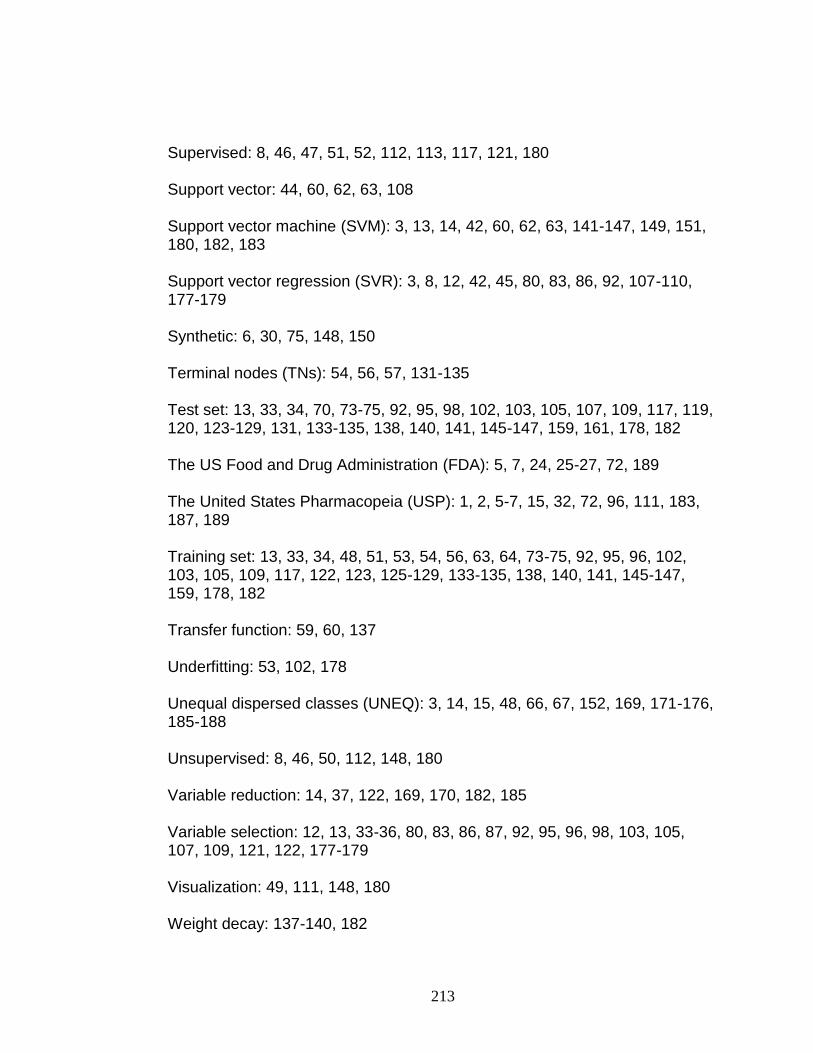
213
Supervised: 8, 46, 47, 51, 52, 112, 113, 117, 121, 180 Support vector: 44, 60, 62, 63, 108 Support vector machine (SVM): 3, 13, 14, 42, 60, 62, 63, 141-147, 149, 151, 180, 182, 183 Support vector regression (SVR): 3, 8, 12, 42, 45, 80, 83, 86, 92, 107-110, 177-179 Synthetic: 6, 30, 75, 148, 150 Terminal nodes (TNs): 54, 56, 57, 131-135 Test set: 13, 33, 34, 70, 73-75, 92, 95, 98, 102, 103, 105, 107, 109, 117, 119, 120, 123-129, 131, 133-135, 138, 140, 141, 145-147, 159, 161, 178, 182 The US Food and Drug Administration (FDA): 5, 7, 24, 25-27, 72, 189 The United States Pharmacopeia (USP): 1, 2, 5-7, 15, 32, 72, 96, 111, 183, 187, 189 Training set: 13, 33, 34, 48, 51, 53, 54, 56, 63, 64, 73-75, 92, 95, 96, 102, 103, 105, 109, 117, 122, 123, 125-129, 133-135, 138, 140, 141, 145-147, 159, 178, 182 Transfer function: 59, 60, 137 Underfitting: 53, 102, 178 Unequal dispersed classes (UNEQ): 3, 14, 15, 48, 66, 67, 152, 169, 171-176, 185-188 Unsupervised: 8, 46, 50, 112, 148, 180 Variable reduction: 14, 37, 122, 169, 170, 182, 185 Variable selection: 12, 13, 33-36, 80, 83, 86, 87, 92, 95, 96, 98, 103, 105, 107, 109, 121, 122, 177-179 Visualization: 49, 111, 148, 180 Weight decay: 137-140, 182