discrete-time stochastic models, sdes, and numerical methods

DISCRETE-TIME STOCHASTIC MODELS, SDEs, ANDNUMERICAL METHODS

Ed Allen

NIMBioS Tutorial: Stochastic Models With BiologicalApplications

University of Tennessee, Knoxville

March, 2011

ACKNOWLEDGEMENT

I thank all the participants for their time and their interest

in stochastic modeling in biology.

I thank Professor Louis Gross and Professor Suzanne Lenhart

for requesting and funding this tutorial.

STOCHASTIC DIFFERENTIAL EQUATIONS AREBECOMING INCREASINGLY MORE POPULAR

(1) Random effects in biological, physical, and financial prob-lems can be modeled using stochastic differential equations.

(2) Stochastic models are considered to be more realistic formany problems.

(3) A procedure for deriving accurate stochastic differentialequation models is useful to understand.

(4) For simulating stochastic differential equations, computa-tional procedures are generally necessary.

This Lecture Is Divided Into Several Parts

(1) A procedure is described for deriving a stochastic differen-tial equation from an associated discrete stochastic model.

(2) Stochastic differential equation systems are derived for sev-eral population problems. (Modeling with SDEs continues inthe second lecture.)

(3) Commonly used numerical procedures are described forcomputationally solving systems of stochastic differential equa-tions.

To Introduce SDE Modeling, Consider The Birth-DeathProcess

Let u(t) be the population size and let b and d be birth and deathrates. The dynamics of the birth-death process is representedexactly by:

u(t + (∆t)t) = u(t) + (∆u)t, u(0) = a

where (∆t)t is the time interval to the next birth or death aftertime t, (∆u)t = 1 with probability b/(b + d), and (∆u)t = −1 withprobability d/(b + d).

In addition, (∆t)t is exponentially distributed and if βt is arandom number uniform on [0, 1], then

(∆t)t = − log (βt)/((b + d)u(t)).

The above is suitable for Monte Carlo computations, but theseequations give little insight into the birth-death process.

A Deterministic ODE Model Is Often Used For TheBirth-Death Process

Since E(u(t + ∆t)) = E(u(t)) + (b − d)E(u(t))∆t for small ∆t, it fol-lows that

dv(t)

dt= (b − d)v(t), v(0) = a.

where v(t) = E(u(t)).

This ODE is so common and so well-accepted that it is oftenforgotten that there are two important assumptions:

(1) v(t) is not the population size; it is the mean size, and

(2) v(t) varies continuously, i.e., the population size can havefractional values.

In this model, we have lost information about the randomnessin the birth-death process and about the population’s integersize values.

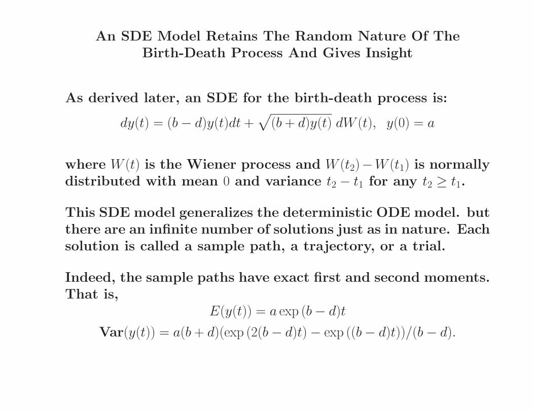
An SDE Model Retains The Random Nature Of TheBirth-Death Process And Gives Insight

As derived later, an SDE for the birth-death process is:

dy(t) = (b − d)y(t)dt +√

(b + d)y(t) dW (t), y(0) = a

where W (t) is the Wiener process and W (t2)−W (t1) is normallydistributed with mean 0 and variance t2 − t1 for any t2 ≥ t1.

This SDE model generalizes the deterministic ODE model. butthere are an infinite number of solutions just as in nature. Eachsolution is called a sample path, a trajectory, or a trial.

Indeed, the sample paths have exact first and second moments.That is,

E(y(t)) = a exp (b − d)t

Var(y(t)) = a(b + d)(exp (2(b − d)t) − exp ((b − d)t))/(b − d).

Calculations Indicate That An SDE For The Birth-DeathProcess Is Very Reasonable

0 1 2 3 40

20

40

60

80

100

Time t

Po

pu

latio

n S

ize

A Monte Carlo Path, An SDE Path, and the Average Path

0 1 2 3 40

20

40

60

80

100

Time t

Po

pu

latio

n S

ize

A Monte Carlo Path, An SDE Path, and the Average Path

Figure 1: Calculated Sample Paths for a Birth-Death Process where b=1.0 and d=0.5

The SDE captures the random behavior of the birth-death pro-cess even though the population values are not integers.

For SDEs, It Is Very Useful To Understand Wiener Processes

The Wiener process satisfies certain properties:

(a) W (0) = 0,

(b) W (t) ∼ N(0, t), that is, W (t) is distributed normally withmean 0 and variance t for each t,

(c) W (t + ∆t) − W (t) ∼ N(0, ∆t) for each t and each ∆t,

(d) the Wiener process can be generated by the recurrence:

W ((k+1)∆t) = W (k∆t)+√

∆t ηk for k = 0, 1, 2, . . . and ηk ∼ N(0, 1),

(e) W (t3) − W (t2) is independent of W (t2) − W (t1) for t1 < t2 < t3.Indeed,

E(W (t3)−W (t2))(W (t2)−W (t1)) = 0 but E(W (t2)−W (t1))2 = t2−t1.

(f) the Wiener process is continuous but nowhere differen-tiable.

Generation of a Wiener process gives some understanding

A sample path of a Wiener process W (t) can be easily gener-ated at a finite number of points.

Suppose that a Wiener process trajectory is desired on the in-terval [t0, tN ] at the points {ti}N

i=0 where t0 = 0. Then, W (t0) = 0and

W (ti) = W (ti−1) + ηi−1

√

ti − ti−1, for i = 1, 2, . . . , N,

where ηi−1 are independent normally distributed numbers.

The values W (ti), i = 0, 1, . . . , N , determine a Wiener samplepath at the points {ti}N

i=0.

(Note that the normally distributed random numbers, ηi−1 fori = 1, 2, . . . , N , are generally found using pseudo-random numbergenerators.)

Two Sample Paths (Or Trajectories) Of The Wiener ProcessIllustrate Its Random Behavior

0 0.2 0.4 0.6 0.8 1−2

−1.5

−1

−0.5

0

0.5

1

1.5

2

Time t

Wie

ner P

roce

sses

Figure 2: Two Wiener Processes On [0,1]

SDEs Are Defined From Stochastic Integrals

The Ito integral∫ b

a f (t) dW (t) is defined to be

∫ b

a

f (t) dW (t) = limm→∞

m−1∑

i=0

f (ti)(

W (ti+1) − W (ti))

where ti = a + i∆t and ∆t = (b − a)/m.

Two useful properties are:

(1) E(∫ b

a f (t) dW (t)) = 0

(2) E(∫ b

a f (t) dW (t))2 =∫ b

a E(f (t))2 dt

In addition, if X(t) =∫ t

0 f (t) dt +∫ t

0 g(t) dW (t), we say that X(t)satisfies the Ito SDE:

dX(t)

dt= f (t) + g(t)

dW (t)

dtor dX(t) = f (t) dt + g(t) dW (t).

Ito Stochastic Differential Equations Are Popular

An Ito SDE has the form

X(t) = X(0) +

∫ t

0

f (s, X(s)) ds +

∫ t

0

g(s, X(s)) dW (s)

for 0 ≤ t ≤ T where X(0) is given.

In differential form,

dX(t) = f (t, X(t)) dt + g(t, X(t)) dW (t)

where f is called the drift coefficient and g is called the diffu-sion coefficient.

To prove existence and uniqueness, it is often assumed that fand g satisfy:

Condition (a): |f (t, x)−f (s, y)|2 ≤ k(|t−s|+ |x−y|2) for 0 ≤ s, t ≤ Tand x, y ∈ R.

Condition (b): |f (t, x)|2 ≤ k(1 + |x|2) for 0 ≤ t ≤ T and x ∈ R.

Solutions of the SDE are Bounded and Continuous

Assuming that f and g satisfy (a) and (b) then there are con-stants c1 and c2 such that:

Boundedness:

E|X(t)|2 ≤ c1 for 0 ≤ t ≤ T.

Continuity:

E|X(t) − X(r)|2 ≤ c2|t − r| for 0 ≤ r, t ≤ T.

(So, given ε > 0 there is a δ > 0 such that (E|X(t)−X(r)|2)1/2 < εwhen |t − r| < δ.)

Ito’s Formula Is Very Useful To Understand

Ito’s formula says that a smooth function, F (t, X(t)), of thestochastic process X(t) also satisfies an SDE.

Consider the Ito SDE in differential form:

dX(t) = f (t, X(t)) dt + g(t, X(t)) dW (t) for 0 ≤ t ≤ T.

Let F be a smooth function. Ito’s formula says:

dF (t, X(t)) =

(

∂F (t,X)

∂t+ f (t, X)

∂F (t, X)

∂x+

1

2g2(t,X)

∂2F (t, X)

∂x2

)

dt

+ g(t, X)∂F (t, X)

∂xdW (t).

Ito’s formula helps us, for example, determine exact solutionsor moments for certain SDEs. In doing this, useful is:

E

(∫ t

0

G(t, X(t)) dW (t)

)

= 0.

SKETCH OF A PROOF OF ITO’S FORMULA

The proof of Ito’s formula relies on using the Taylor seriesexpansion to o(∆t):

F (t + ∆t, X(t + ∆t)) − F (t, X(t)) ≈ ∂F (t, X)

∂t∆t +

+∂F (t,X)

∂X(X(t + ∆t) − X(t)) +

1

2

∂2F (t, X)

∂X2(X(t + ∆t) − X(t))2.

Dividing by ∆t and using, also to order o(∆t), the approxima-tion:

X(t + ∆t) − X(t) =

∫ t+∆t

t

f (s)ds +

∫ t+∆t

t

g(s)dW (s) ≈ f (t)∆t + g(t)∆W,

we obtain that:

dF (t, X(t))

dt=

∂F (t, X)

∂t+

∂F (t, X)

∂X

(

f (t) + g(t)dW (t)

dt

)

+1

2

∂2F (t, X)

∂X2g2(t)

where we used

E(∆W )2 = E(W (t + ∆t) − W (t))2 = ∆t.

Example: Finding Exact Moments For An SDE

Consider the SDE:

dX(t) = −1

4X3(t) dt +

1

2X2(t) dW (t) with X(0) =

1

2.

In this example, E(X(t)) and E(X3(t)) are to be determined ex-actly.

First,

dE(X(t)) = −1

4E(X3(t)) dt with E(X(0)) =

1

2so E(X3(t)) is needed in order to find E(X(t)). Applying Ito’sformula to the SDE gives

dX3(t) =

[

−3

4X5(t) +

3

4X5(t)

]

dt +3

2X4(t) dW (t) =

3

2X4(t) dW (t)

with E(X3(0)) =1

8.

Thus, E(X3(t)) =1

8and it follows that E(X(t)) =

1

2− 1

32t.

Example: Finding Exact Moments For An SDE

Consider the stochastic differential equation

dX(t) =

[

1

3X1/3(t) + 6X2/3(t)

]

dt + X2/3(t) dW (t) with X(0) = 1.

In this example, we wish to determine E(X(t)) and E(X2(t))exactly. First notice that

dE(X(t)) 6=[

1

3

(

E(X(t)))1/3

+ 6(

E(X(t)))2/3

]

dt

so an appropriate change of variables is required to find themoments. Let

Yn(t) = (X(t))n/3 for n = 0, 1, 2, . . . , 6.

Next, applying Ito’s formula, the stochastic differentials areobtained

dYn(t) =

[

1

18(n2 − n)X

n−23 (t) + 2nX

n−13 (t)

]

dt +[n

3X

n−13 (t)

]

dW (t)

with Yn(0) = 1 for n = 0, 1, 2, . . . , 6. Then,

dYn(t) =

[

1

18(n2 − n)Yn−2(t) + 2nYn−1(t)

]

dt +[n

3Yn−1(t)

]

dW (t)

for n = 0, 1, 2, . . . , 6.

Letting Zn(t) = E(Yn(t)) = E((X(t))n/3), then the initial-value sys-tem is:

dZn(t)

dt=

1

18(n2 − n)Zn−2(t) + 2nZn−1(t) for n = 1, 2, . . . , 6

with Zn(0) = 1 for n = 1, 2, . . . , 6 and Z0(t) = 1. Solving this gives

Z1(t) = E((X(t))1/3) = 2t + 1

Z2(t) = E((X(t))2/3) = 4t2 +37

9t + 1

Z3(t) = E((X(t)) = 8t3 +38

3t2 +

19

3t + 1

Z6(t) = E((X(t))2) = 64t6 +656

3t5 +

2660

9t4 +

49145

243t3 +

665

9t2 +

41

3t + 1.

In particular, E(X(1)) = 28.0 and E(X2(1)) = 869.0206.

Example: Finding The Exact Solution Of An SDE

Consider the SDE (Ornstein-Uhlenbeck):

dX(t) = β(Xe − X(t)) dt + α dW (t), X(0) = X0

where β, α, Xe, and X0 are constants. Let F (t, X) = eβtX(t). ByIto’s formula,

d(

eβtX(t)))

=[

βeβtX(t) + βeβt(Xe − X(t)]

dt + αeβt dW (t)

Thus,

eβtX(t) − X0 = eβtXe − Xe +

∫ t

0

eβsα dW (s).

So the exact solution is

X(t) = Xe + (X0 − Xe)e−βt + e−βt

∫ t

0

eβsα dW (s)

and, at large time t, X(t) is approximately normally distributedwith mean Xe and variance α2/(2β).

Example: Finding The Exact Solution Of An SDE


dX(t) = f (t)X(t) dt + g(t)X(t) dW (t), X(0) = X0

where X0 is a constant. For this problem, the exact solutionhas the form

X(t) = X0 exp

(∫ t

0

(

f (s) − 1

2g2(s)

)

ds +

∫ t

0

g(s) dW (s)

)

.

To see this, let F (t, X) = ln(X(t)). Applying Ito’s formula,

d(ln(X(t))) =[

f (t) − 1

2g2(t)

]

dt + g(t) dW (t).

Thus,

ln(X(t)) − ln(X0) =

∫ t

0

(

f (s) − 1

2g2(s)

)

ds +

∫ t

0

g(s) dW (s)

which yields the solution.

The Forward Kolmogorov Equation Is Useful To Understand

The probability distribution of solutions to a discrete-valuedcontinuous stochastic process satisfies a system of differentialequations called the forward Kolmogorov equations. An anal-ogous result holds for the probability distribution of solutionsto an SDE. The probability distribution of solutions to an SDEsatisfies a PDE called the forward Kolmogorov equation.


dX(t) = f (t, X(t)) dt + g(t, X(t)) dW (t).

By applying Ito’s formula, it can be shown that the probabilitydensity for solutions to the SDE satisfies:

∂p(t, x)

∂t= −∂(p(t, x)f (t, x))

∂x+

1

2

∂2(p(t, x)g2(x, t))

∂2x.

In particular, P (a < X(t) < b) =∫ b

a p(x, t) dx.

SKETCH OF A PROOF OF THE FORWARD KOLMOGOROV EQUA-

TION


dX(t) = f (t, X(t)) dt + g(t, X(t)) dW (t)

and let F ∈ C∞0 (R). Applying Ito’s formula to F (X) gives

dF (X) =

(

f (t, X)∂F (t, X)

∂x+

1

2g2(t,X)

∂2F (t, X)

∂x2

)

dt

+ g(t, X)∂F (t, X)

∂xdW (t).

Because

E

∫ t

0

g(s, X(s))∂F (X(s))

∂xdW (s) = 0,

thendE(F )

dt= E

[

∂F

∂xf +

1

2g2∂

2F

∂x2

]

.

Let p(t, x) be probability density for solutions to the SDE. Then,

d

dt

∫ ∞

−∞p(t, x)F (x) dx =

∫ ∞

−∞p(t, x)

[

∂F

∂xf +

1

2g2∂

2F

∂2x

]

dx.

Integrating by parts the right-hand side yields∫ ∞

−∞F (x)

[

∂p(t, x)

∂t+

∂(p(t, x)f (t, x))

∂x− 1

2

∂2(p(t, x)g2(t, x))

∂2x

]

dx = 0.

As the above integral holds for every function F ∈ C∞0 (R), this

implies that

∂p(t, x)

∂t= −∂(p(t, x)f (t, x))

∂x+

1

2

∂2(p(t, x)g2(x, t))

∂2x.

This equation is the forward Kolmogorov equation or Fokker-Planck equation for the probability distribution of solutions tothe SDE.

Also, the forward Kolmogorov equation for a system of SDEsis:

∂p(t, ~x)

∂t= −

d∑

i=1

∂[

p(t, ~x)fi(t, ~x)]

∂xi

+1

2

d∑

i=1

d∑

j=1

m∑

l=1

∂2

∂xi∂xj

[

gi,l(t, ~x)gj,l(t, ~x)p(t, ~x)]

.

EXAMPLE: SOLUTION OF A FORWARD KOLMOGOROV EQUATION

Consider the stochastic differential equation{

dX(t) = a dt + b dW (t)X(0) = x0.

The probability density of the solutions satisfies the forwardKolmogorov equation

∂p(t, x)

∂t= −∂(ap(t, x))

∂x+

b2

2

∂2(p(t, x))

∂2xp(0, x) = δ(x − x0).

The solution to this partial differential equation is

p(t, x) =1√

2πb2texp

(−(x − at − x0)2

2b2t

)

.

Numerical Methods To Approximate SDEs Are Valuable

The exact solution to an SDE is generally difficult to obtainso methods to approximate the solution are important. TheEuler-Maruyama method is the most commonly used numeri-cal method.

The Euler-Maruyama method has the form

Xi+1 = Xi + f (ti, Xi)∆t + g(ti, Xi)∆Wi, X0 = X(0)

for i = 0, 1, 2, . . . , N − 1 where Xi ≈ X(ti), ti = i∆t, ∆t = T/N ,∆Wi = (W (ti+1) − W (ti)) ∼ N(0, ∆t).

To study the error in this method, we approximate the solu-tion for all t ∈ [0, T ] and not just at the nodal points ti. Toaccomplish this, let X(t) ≈ X(t) be defined as

X(t) = Xi +

∫ t

ti

f (ti, Xi) ds +

∫ t

ti

g(ti, Xi) dW (s)

for ti ≤ t ≤ ti+1 and i = 0, 1, . . . , N − 1. Notice that X is identicalto Euler’s method approximation at the nodal points, that is,X(ti) = Xi for i = 0, 1, . . . , N .

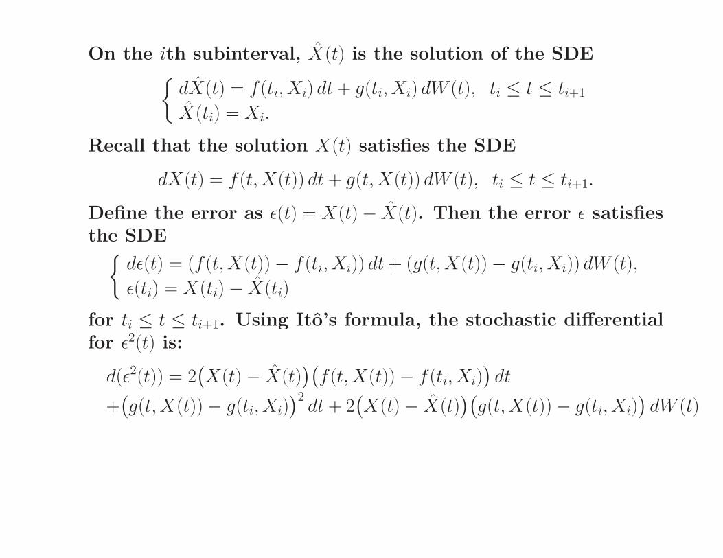
On the ith subinterval, X(t) is the solution of the SDE{

dX(t) = f (ti, Xi) dt + g(ti, Xi) dW (t), ti ≤ t ≤ ti+1

X(ti) = Xi.

Recall that the solution X(t) satisfies the SDE

dX(t) = f (t, X(t)) dt + g(t, X(t)) dW (t), ti ≤ t ≤ ti+1.

Define the error as ε(t) = X(t) − X(t). Then the error ε satisfiesthe SDE

{

dε(t) = (f (t, X(t)) − f (ti, Xi)) dt + (g(t, X(t)) − g(ti, Xi)) dW (t),

ε(ti) = X(ti) − X(ti)

for ti ≤ t ≤ ti+1. Using Ito’s formula, the stochastic differentialfor ε2(t) is:

d(ε2(t)) = 2(

X(t) − X(t))(

f (t, X(t)) − f (ti, Xi))

dt

+(

g(t, X(t)) − g(ti, Xi))2

dt + 2(

X(t) − X(t))(

g(t, X(t)) − g(ti, Xi))

dW (t)

Hence, E(ε2(ti+1)) satisfies

E(ε2(ti+1)) = E(ε2(ti)) + E

∫ ti+1

ti

(

g(t, X(t)) − g(ti, Xi))2

dt

+ E

∫ ti+1

ti

2(

X(t) − X(t))(

f (t, X(t)) − f (ti, Xi))

dt

+ E

∫ ti+1

ti

2(

X(t) − X(t))(

g(t, X(t)) − g(ti, Xi))

dW (t)

Using the inequality |2ab| ≤ a2 + b2 and properties of stochasticintegrals,

E(ε2(ti+1)) ≤ E(ε2(ti)) +

∫ ti+1

ti

E(X(t) − X(t))2 dt

+

∫ ti+1

ti

E(f (t, X(t)) − f (ti, Xi))2 dt +

∫ ti+1

ti

E(g(t, X(t)) − g(ti, Xi))2 dt.

But

|f (t, X(t)) − f (ti, Xi)|2 ≤ 2|f (t, X(t)) − f (ti, X(ti))|2+2|f (ti, X(ti)) − f (ti, Xi)|2

≤ 2k|t − ti| + 2k|X(t) − X(ti)|2 + 2k|X(ti) − Xi|2

and similarly for g. Hence,

E(ε2(ti+1)) ≤ E(ε2(ti)) +

∫ ti+1

ti

E(X(t) − X(t))2 dt

+4k(1 + c)

∫ ti+1

ti

(t − ti) dt + 4k

∫ ti+1

ti

E(ε2(ti)) dt

using E|X(t) − X(ti)|2 ≤ c|t − ti|. Therefore,

E(ε2(ti+1)) ≤ E(ε2(ti))(1 + 4k∆t) + 2k(1 + c)(∆t)2 +

∫ ti+1

ti

E(ε2(s)) ds.

By Bellman-Gronwall inequality with b(t) = E(ε2(ti))(1 + 4k∆t)+2k(1 + c)(∆t)2,

E(ε2(ti+1)) ≤ E(ε2(ti))(1 + 4k∆t) + 2k(1 + c)(∆t)2

+

∫ ti+1

ti

e(ti+1−t)[

E(ε2(ti))(1 + 4k∆t) + 2k(1 + c)(∆t)2]

dt

= e∆t[

E(ε2(ti))(1 + 4k∆t) + 2k(1 + c)(∆t)2]

.

Letting ai = E(ε2(ti)), R = e∆t(1 + 4k∆t), and S = e∆t2k(1 + c)(∆t)2,then

ai+1 ≤ Rai + S for i = 0, 1, 2, . . . , N − 1.

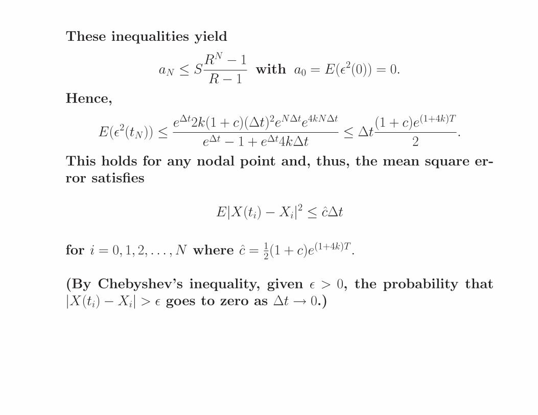
These inequalities yield

aN ≤ SRN − 1

R − 1with a0 = E(ε2(0)) = 0.

Hence,

E(ε2(tN)) ≤ e∆t2k(1 + c)(∆t)2eN∆te4kN∆t

e∆t − 1 + e∆t4k∆t≤ ∆t

(1 + c)e(1+4k)T

2.

This holds for any nodal point and, thus, the mean square er-ror satisfies

E|X(ti) − Xi|2 ≤ c∆t

for i = 0, 1, 2, . . . , N where c = 12(1 + c)e(1+4k)T .

(By Chebyshev’s inequality, given ε > 0, the probability that|X(ti) − Xi| > ε goes to zero as ∆t → 0.)

Milstein’s Method Is A Well-Known Higher-Order Method

Higher order numerical methods for SDEs are similar to higherorder methods for ODEs. For example, there are explicit orimplicit multistep methods and Runge-Kutta methods.

A popular second-order method is Milstein’s method and hasmean square error proportional to (∆t)2 rather than ∆t. Mil-stein’s method has the form

Xi+1 = Xi + f (ti, Xi)∆t + g(ti, Xi)∆Wi

+1

2g(ti, Xi)

∂g(ti, Xi)

∂x[(∆Wi)

2 − ∆t]

for i = 0, 1, 2, . . . , N − 1 with X0 = X(0, ), where Xi ≈ X(ti),∆Wi = (W (ti+1) − W (ti)) ∼ N(0, ∆t), ti = i∆t, ∆t = T/N .

Milstein’s method has an additional term at each step in com-parison with Euler’s method.

Example: Approximation Of An SDE By Euler-MaruyamaAnd By Milstein


dX(t) =

[

1

3X1/3(t) + 6X2/3(t)

]

dt + X2/3(t) dW (t), X(0) = 1.

It was shown earlier that E(X(1)) = 28.0 and E(X2(1)) = 869.0206.For this problem, Euler’s method has the form:

Xi+1 = Xi +

[

1

3X

1/3i + 6X

2/3i

]

∆t + X2/3i

√∆t ηi where ηi ∼ N(0, 1)

for i = 0, 1, 2, . . . , N − 1 with X0 = 1, ti = i∆t, and ∆t = 1/N .Milstein’s method has the form

Xi+1 = Xi +

[

1

3X

1/3i + 6X

2/3i

]

∆t + X2/3i

√∆t ηi +

1

3X

1/3i (η2

i − 1)∆t

where ηi ∼ N(0, 1).

The calculational results for the mean square error E|X(1)−XN |2are given in the table for 10,000 sample paths for each valueof N .

Value of N Euler Error Milstein Error

29 2.80 × 10−2 1.61 × 10−2

210 1.04 × 10−2 4.03 × 10−3

211 4.20 × 10−3 1.01 × 10−3

212 1.89 × 10−3 2.53 × 10−4

213 8.76 × 10−4 6.24 × 10−5

214 4.12 × 10−4 1.60 × 10−5

Notice that the mean square errors are approximately propor-tional to ∆t = 1/N for Euler’s method and to (∆t)2 = 1/N 2 forMilstein’s method.

0 0.2 0.4 0.6 0.8 10

5

10

15

20

25

30

Time

Mea

n an

d O

ne S

ampl

e P

ath

Figure 3: Mean solution and one sample path

The mean and one sample path are plotted in the figure forthis problem.

Next, for this example, E(X(1)) and E(X(1))2 were estimated us-

ing E(X(1)) ≈∑100,000

j=1 X(j)N /100, 000 and E(X(1))2 ≈

∑100,000j=1 (X

(j)N )2/100, 000

where X(j)N is the estimate of X(1) for the jth sample path using

N intervals.

In the table, the errors are given in parentheses. Recall thatE(X(1)) = 28.0 and E(X2(1)) = 869.0206 are the exact values. No-tice that the errors in the mean values are proportional to ∆tfor either numerical method. In particular, the errors in Eu-ler’s method when estimating mean values are proportional to∆t rather than (∆t)1/2.

Value of N Euler Estimate Milstein Estimate

26 27.07 (0.93) 27.08 (0.92)27 27.56 (0.44) 27.56 (0.44)28 27.79 (0.21) 27.79 (0.21)

Value of N Euler Estimate Milstein Estimate

26 810.15 (58.87) 810.18 (58.84)27 840.89 (28.13) 840.93 (28.09)28 855.33 (13.69) 855.31 (13.71)

There Are Two Forms of Approximation: Strong And Weak

This example illustrates that are two kinds of approximationin computational solution of SDEs.

A method is a strong approximation of order γ if

(E(X(T ) − XN)2)1/2 ≤ c(∆t)γ

where X(T ) is the exact solution at time T and XN is the ap-proximate solution.Euler’s and Milstein’s methods have strong orders 1

2 and 1.

However, if expectations of functions for an SDE are desiredand not necessarily the pathwise approximation of a strong ap-proximation, then a weak numerical method may be sufficient.

An approximation XN is said to converge weakly with order βif

|E(F (X(T ))) − E(F (XN))| ≤ c(∆t)β

for all smooth functions F .Euler’s and Milstein’s method both have weak order 1.

Richardson Extrapolation Can Increase The Accuracy OfWeak Approximations

Both Euler’s or Milstein’s method have weak-error expansionsof the correct form for applying Richardson extrapolation.

The weak error for Euler’s or Milstein’s method has the form

E(F (X(T ))) − E(F (XN)) = c1∆t + c2(∆t)2 + c3(∆t)3 + . . . ,

where ∆t = T/N and c1, c2, c3, . . . are independent of ∆t.

Several approximations with different values of N can be ap-plied to obtain a higher order approximation. Suppose thatE(F (XN)), E(F (X2N)), and E(F (X4N)) are three approximationsto E(F (X(T ))) using step lengths of T/N , T/2N , and T/4N inEuler’s or in Milstein’s method.

To obtain an approximation to E(F (X(T ))) of order (∆t)2, let

E(F (X(T ))) −[

2E(F (X2N)) − E(F (XN))]

= c2(∆t)2 + c3(∆t)3 + . . . .

To obtain an approximation to E(F (X(T ))) of order (∆t)3, let

E(F (X(T )))−[

8E(F (X4N))−6E(F (X2N))+E(F (XN))]

/3 = c3(∆t)3+. . . .

An Example Illustrates Richardson Extrapolation

For the previous example, the following approximations toE((X(1))2) are obtained using the Euler-Maruyama method:

E((X64)2) = 810.15, E((X128)

2) = 840.89, and E((X256)2) = 855.33.

To obtain O((∆t)2) and O((∆t)3) approximations, respectively, toE((X(1))2) we calculate

2E((X128)2) − E((X64)

2) = 871.63

and[8E((X256)

2) − 6E((X128)2) + E((X64)

2)]/3 = 869.15.

As E((X(1))2) = 869.02 exactly, the original Euler approximationsare much improved through extrapolation.

Systems Of SDEs Can Be Treated In A Similar Manner

Ito’s formula and numerical methods can be extended to sys-tems. Let

~X(t) = [X1(t), X2(t), . . . , Xd(t)]T

~W (t) = [W1(t),W2(t), . . . , Wm(t)]T

~f : [0, T ] × Rd → R

d and g : [0, T ] × Rd → R

d×m,

where Wi(t), 1 ≤ i ≤ m are independent Wiener processes.

Then a system of stochastic differential equations has the form

d ~X(t) = ~f (t, ~X(t)) dt + g(t, ~X(t)) d ~W (t).

In component form, the system is

Xi(t) = Xi(0) +

∫ t

0

fi(s, ~X(s)) ds +

m∑

j=1

∫ t

0

gi,j(s, ~X(s)) dWj(s)

for i = 1, 2, . . . , d.

Ito’s Formula Generalizes For Systems Of SDEs

Let

~F : [0, T ] × Rd → R

k and let ~Y (t, ω) = ~F (t, ~X(t, ω)).

Then the pth component of ~Y (t, ω) satisfies:

dYp(t) =

∂Fp

∂t+

d∑

i=1

fi∂Fp

∂xi+

d∑

i=1

d∑

j=1

m∑

l=1

1

2gi,lgj,l

∂2Fp

∂xi∂xj

dt

+

m∑

l=1

d∑

i=1

gi,l∂Fp

∂xidWl(t)

for p = 1, 2, . . . , k.

Example of Ito’s Formula For An SDE With d = 1 and m = 2

Consider the SDE:{

dX(t) = t2X(t) dt + t dW1(t) + X(t) dW2(t), 0 ≤ t ≤ TX(0) = 1,

where d = 1 and m = 2.

For this problem, f1 = t2X, g1,1 = t, and g1,2 = X.

Consider using Ito’s formula to find the SDE for F = X2. Ap-plying Ito’s formula,{

d(X2(t)) =[

2t2X2(t) + t2 + X2(t)]

dt + 2tX(t) dW1(t) + 2X2(t) dW2(t)X2(0) = 1.

The Euler-Maruyama And Milstein Methods Extend ToSystems

Euler’s method for systems has the form

~Xn+1(ω) = ~Xn(ω) + ~f (tn, ~Xn(ω))∆t + g(tn, ~Xn(ω))∆ ~Wn(ω)

for n = 0, 1, 2, . . . , N , where ~Xn(ω) ≈ ~X(tn, ω), ∆t = T/N , ∆ ~Wn =~W (tn+1) − ~W (tn).

In component form, Euler’s method is:

Xi,n+1(ω) = Xi,n(ω) + fi(tn, ~Xn(ω))∆t +

m∑

j=1

gi,j(tn, ~Xn(ω))∆Wj,n(ω)

for i = 1, 2, . . . , d, where ∆Wj,n ∼ N(0, ∆t).

Milstein’s method for multidimensional SDEs involves the dou-ble stochastic integral

In(j1, j2) =

∫ tn+∆t

tn

∫ s

tn

dWj1(r) dWj2(s).

Milstein’s method has the componentwise form

Xi,n+1(ω) = Xi,n(ω) + fi(tn, ~Xn(ω))∆t +

m∑

j=1

gi,j(tn, ~Xn(ω))∆Wj,n(ω)

+

m∑

j1=1

m∑

j2=1

d∑

l=1

gl,j1

∂gi,j2

∂xlIn(j1, j2)

for i = 1, 2, . . . , d.

An Example Of Approximation Of An SDE With d = 1 Andm = 2

Consider the SDE;{

dX(t) = t2X(t)dt + tdW1(t) + X(t)dW2(t), 0 ≤ t ≤ TX(0) = 1,

where d = 1 and m = 2.

For this problem, Euler’s method has the form{

Xn+1 = Xn + t2nXn∆t + tn∆W1,n + Xn∆W2,n

X0 = 1,

for n = 0, 1, 2, . . . , where ∆W1,n, ∆W2,n ∼ N(0, ∆t) and tn = n∆t.

Milstein’s method has the form{

Xn+1 = Xn + t2nXn∆t + tn∆W1,n + Xn∆W2,n + tnIn(1, 2) + XnIn(2, 2)X0 = 1,

for n = 0, 1, 2, . . . .

It is useful to note that

In(j1, j1) =

∫ tn+∆t

tn

∫ s

tn

dWj1(r) dWj1(s) =1

2

(

(∆Wj1,n)2 − ∆t

)

but In(j1, j2) for j1 6= j2 does not have an analytical form andmust be approximated.

This multiple integral can be approximated by a Fourier seriesexpansion. Also, if [tn, tn+1] is divided into M equal intervalswith tj,n = tn + j∆t/M for j = 0, 1, . . . , M, then

In(j1, j2) ≈ In(j1, j2) =

M−1∑

j=0

[Wj1(tj,n) − Wj1(t0,n)][Wj2(tj+1,n) − Wj2(tj,n)].

It can be shown that E|In − In|2 = (∆t)2/(2M).

A Procedure For Deriving Accurate SDE Models Is Useful

The derivation procedure is analogous to that used for manyODEs models. Basically,

(1) The process is studied for a small time interval ∆t.

(2) The changes in the process leads to a differential equationmodel.

For example, consider deriving an ODE model for the temper-ature of an object immersed in a liquid held at temperatureTL. Suppose for interval ∆t, the change in the temperature isproportional to the difference between the object’s tempera-ture T (t) and the liquid’s temperature TL.

Based on this, ∆T = α(TL − T (t))∆t where α is a constant.

Setting ∆T = T (t + ∆t) − T (t) and letting ∆t → 0, one obtainsNewton’s Law of Cooling:

dT

dt= α(TL − T ).

The Procedure For Deriving Accurate SDE Models Is Useful

The derivation procedure can be applied to randomly varyingdynamical systems in physics, engineering, and biology and issimilar to stochastic modeling procedures used in chemistry.

In the procedure, a finite ∆t produces a discrete stochasticmodel. The discrete stochastic model then leads to a stochas-tic differential equation model as ∆t → 0. Specifically:

(1) A discrete stochastic model is developed for the randomdynamical system. In particular, for a small time interval ∆t,the possible changes with their corresponding transition prob-abilities are determined.

(2) The expected changes and the covariance matrix for thechanges are determined for the discrete stochastic process.

(3) A stochastic differential equation model is inferred by sim-ilarities in the forward Kolmogorov equations between the dis-crete and continuous stochastic processes.

S1(t) S

2(t)

1 2 3 4

5

6

7 8

THE PROCEDURE IS ILLUSTRATED FOR ATWO-STATE PROBLEM

Let S1(t) and S2(t) represent the values of two states at time t.

It is assumed that in a small time interval ∆t, state S1 canchange by −λ1, 0, or +λ1 and state S2 can change by −λ2, 0, or+λ2 where λ1, λ2 ≥ 0. Let ∆~S = [S1, S2]

T be the change in a smalltime interval ∆t.

The changes and probabilities are listed in the table.

For example, change 1 represents a loss of λ1 in S1(t) with prob-ability d1∆t.

Change 5 represents a transfer of λ1 out of state S1 with a cor-responding transfer of λ2 into state S2 with probability m12∆t.

Change 7 represents a simultaneous reduction in both statesS1 and S2.

Change Probability

∆~S(1) = [−λ1, 0]T p1 = d1(t, S1, S2)∆t

∆~S(2) = [λ1, 0]T p2 = b1(t, S1, S2)∆t

∆~S(3) = [0,−λ2]T p3 = d2(t, S1, S2)∆t

∆~S(4) = [0, λ2]T p4 = b2(t, S1, S2)∆t

∆~S(5) = [−λ1, λ2]T p5 = m12(t, S1, S2)∆t

∆~S(6) = [λ1,−λ2]T p6 = m21(t, S1, S2)∆t

∆~S(7) = [−λ1,−λ2]T p7 = m11(t, S1, S2)∆t

∆~S(8) = [λ1, λ2]T p8 = m22(t, S1, S2)∆t

∆~S(9) = [0, 0]T p9 = 1 −∑8

i=1 pi

Derivation Of An SDE For A Two-State Problem Continues

We calculate the expected change and the covariance matrixfor the change ∆~S = [∆S1, ∆S2]

T . Using the table,

E(∆~S) =

9∑

j=1

pj∆~S(j) =

(−d1 + b1 − m12 + m21 + m22 − m11)λ1

(−d2 + b2 + m12 − m21 + m22 − m11)λ2

∆t

and

E(∆~S(∆~S)T ) =

9∑

j=1

pj(∆~S(j))(∆~S(j))T =

=

(d1 + b1 + ma)λ21 (−m12 − m21 + m22 + m11)λ1λ2

(−m12 − m21 + m22 + m11)λ1λ2 (d2 + b2 + ma)λ22

∆t

where ma = m12 + m21 + m22 + m11.

Let ~µ(t, S1, S2) = E(∆~S)/∆t and V (t, S1, S2) = E(∆~S(∆~S)T )/∆t.

As ∆t is small and E(∆~S)(E(∆~S))T = O((∆t)2), the covariance

matrix V is set equal to E(∆~S(∆~S)T )/∆t. Finally, define thesquare root of the covariance matrix V as B:

B(t, S1, S2) = (V (t, S1, S2))1/2 and thus, B2(t, S1, S2) = V (t, S1, S2).

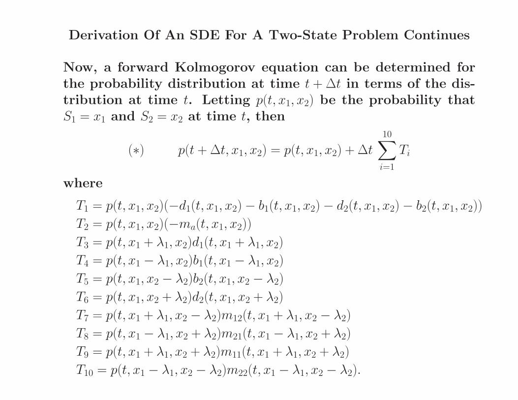
Derivation Of An SDE For A Two-State Problem Continues

Now, a forward Kolmogorov equation can be determined forthe probability distribution at time t + ∆t in terms of the dis-tribution at time t. Letting p(t, x1, x2) be the probability thatS1 = x1 and S2 = x2 at time t, then

(∗) p(t + ∆t, x1, x2) = p(t, x1, x2) + ∆t10

∑

i=1

Ti

where

T1 = p(t, x1, x2)(−d1(t, x1, x2) − b1(t, x1, x2) − d2(t, x1, x2) − b2(t, x1, x2))

T2 = p(t, x1, x2)(−ma(t, x1, x2))

T3 = p(t, x1 + λ1, x2)d1(t, x1 + λ1, x2)

T4 = p(t, x1 − λ1, x2)b1(t, x1 − λ1, x2)

T5 = p(t, x1, x2 − λ2)b2(t, x1, x2 − λ2)

T6 = p(t, x1, x2 + λ2)d2(t, x1, x2 + λ2)

T7 = p(t, x1 + λ1, x2 − λ2)m12(t, x1 + λ1, x2 − λ2)

T8 = p(t, x1 − λ1, x2 + λ2)m21(t, x1 − λ1, x2 + λ2)

T9 = p(t, x1 + λ1, x2 + λ2)m11(t, x1 + λ1, x2 + λ2)

T10 = p(t, x1 − λ1, x2 − λ2)m22(t, x1 − λ1, x2 − λ2).

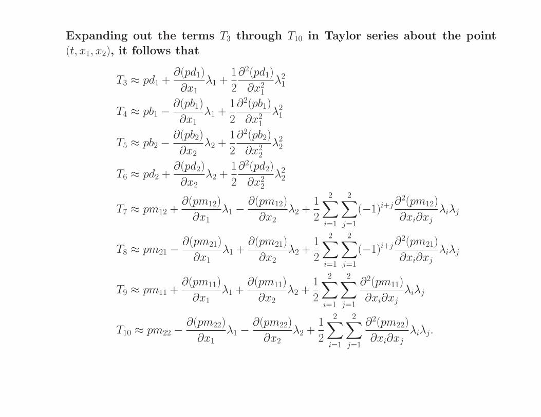
Expanding out the terms T3 through T10 in Taylor series about the point

(t, x1, x2), it follows that

T3 ≈ pd1 +∂(pd1)

∂x1λ1 +

1

2

∂2(pd1)

∂x21

λ21

T4 ≈ pb1 −∂(pb1)

∂x1λ1 +

1

2

∂2(pb1)

∂x21

λ21

T5 ≈ pb2 −∂(pb2)

∂x2λ2 +

1

2

∂2(pb2)

∂x22

λ22

T6 ≈ pd2 +∂(pd2)

∂x2λ2 +

1

2

∂2(pd2)

∂x22

λ22

T7 ≈ pm12 +∂(pm12)

∂x1λ1 −

∂(pm12)

∂x2λ2 +

1

2

2∑

i=1

2∑

j=1

(−1)i+j∂2(pm12)

∂xi∂xjλiλj

T8 ≈ pm21 −∂(pm21)

∂x1λ1 +

∂(pm21)

∂x2λ2 +

1

2

2∑

i=1

2∑

j=1

(−1)i+j∂2(pm21)

∂xi∂xjλiλj

T9 ≈ pm11 +∂(pm11)

∂x1λ1 +

∂(pm11)

∂x2λ2 +

1

2

2∑

i=1

2∑

j=1

∂2(pm11)

∂xi∂xjλiλj

T10 ≈ pm22 −∂(pm22)

∂x1λ1 −

∂(pm22)

∂x2λ2 +

1

2

2∑

i=1

2∑

j=1

∂2(pm22)

∂xi∂xjλiλj.

Substituting these expressions into (∗) and assuming that ∆t, λ1, and λ2 are

small, then p(t, x1, x2) approximately solves the Fokker-Planck equation

∂p(t, x1, x2)

∂t= −

2∑

i=1

∂

∂xi[µi(t, x1, x2)p(t, x1, x2)]

+1

2

2∑

i=1

2∑

j=1

∂2

∂xi∂xj

[

2∑

k=1

bi,k(t, x1, x2)bj,k(t, x1, x2)p(t, x1, x2)

]

,

where µi is the ith component of ~µ and bi,j = (B)i,j for 1 ≤ i, j ≤ 2.

However, the probability distribution p(t, x1, x2) that exactly satisfies this

PDE is identical to the distribution of solutions to the SDE system{

d~S(t) = ~µ(t, S1, S2) dt + B(t, S1, S2) d ~W (t)~S(0) = ~S0,

where ~W (t) = [W1(t), W2(t)]T .

Therefore, the discrete stochastic model is closely related to an SDE. In

particular, the drift and diffusion terms, ~µ and B, of the SDE are equal to

the expected change divided by ∆t and the square root of the covariance

matrix divided by ∆t from the discrete stochastic model.

DERIVATION OF ACCURATE SDE MODELS

In summary, the derivation procedure in deriving an SDE requires three

steps:

First, a discrete stochastic model for the process is developed by carefully

listing the possible changes along with the corresponding probabilities for

a short time step ∆t.

Second, the expected change and covariance matrix for the change is cal-

culated for the discrete stochastic process.

Third, the stochastic differential equation system is obtained by letting the

expected change divided by ∆t be the drift coefficient and the square root

of the covariance matrix divided by ∆t be the diffusion coefficient.

Note that the derivation procedure provides an Ito SDE rather than, for

example, a Stratonovich SDE.

AN ITO OR A STRATONOVICH SDE

There have been discussions regarding whether an Ito or a Stratonovich

SDE is most appropriate for a given random dynamical system. Whether

the SDE is regarded as Ito or Stratonovich is important. For example, if

dX(t) = λX(t) dt + µX(t) dW (t)

is regarded as Ito, then X(t) → X(0) exp((λ−µ2/2)t) w.p.1 as t → ∞ and, thus,

X(t) → 0 with probability 1 if λ < µ2/2. On the other hand, if this SDE is

Stratonovich, then the equivalent Ito SDE is

dX(t) = (λ + µ2/2)X(t) dt + µX(t) dW (t).

In this case, X(t) → X(0) exp(λt) w.p.1 as t → ∞ and, thus, X(t) → 0 with

probability 1 if λ < 0. Thus, specification of the SDE model as Ito or

Stratonovich is important.

In the derivation procedure, a discrete stochastic model is first developed.

An Ito SDE is then inferred by the similarities between the forward Kol-

mogorov equations of the discrete-time and the continuous-time models.

However, if desired, the Ito SDE can be transformed into a Stratonovich

SDE.

CALCULATING SQUARE ROOTS OF MATRICES

The derivation procedure produces a term in the SDE system that involves

the square root of a symmetric positive definite matrix, that is, B = V 1/2.

Solution of the stochastic system involves computation of square roots of

matrices.

For a 2 × 2 matrix, the square root can be readily calculated. Indeed,

V 1/2 =

a b

b c

1/2

=1

d

a + w b

b c + w

,

where w =√

ac − b2 and d =√

a + c + 2w. However, for a general n × n sym-

metric positive definite matrix V with n ≥ 3, there is no formula for V 1/2

and it must be calculated numerically.

If V is put in the canonical form V = P TDP , where P TP = I and dii > 0

for i = 1, 2, . . . , n, then V 1/2 = P TD1/2P . However, for a large matrix, it is

computationally intensive to accurately compute all of the eigenvalues and

eigenvectors of V which are needed to determine P and D. Fortunately,

there are available many numerical procedures for computing V 1/2 directly.

AN ALTERNATIVE TO SQUARE ROOTS OF MATRICES

Often, the square root of the covariance matrix B = V 1/2 can be avoided by

including additional Wiener processes in the stochastic system.

Consider a stochastic problem that involves N states S1, S2, . . . , SN with a

total of M ≥ N possible random changes to these states at each time step

∆t. Suppose that the probabilities of the changes are pj∆t = pj(t, ~S)∆t for

j = 1, 2, . . . , M where the jth change alters the ith state by the amount λji

for i = 1, 2, . . . , N . The ith element of vector ~µ for this problem is then

µi =

M∑

j=1

pjλji for i = 1, 2, . . . , N.

The covariance matrix, V , can also be computed and the i, l entry of V has

the form

vil =

M∑

j=1

pjλjiλjl for 1 ≤ i, l ≤ N.

However, it is generally difficult to compute the N × N matrix V 1/2 in the

SDE system

d~S = ~µ dt + V 1/2 d ~W (t),

where ~W (t) is a vector consisting of N independent Wiener processes.

AN ALTERNATIVE TO SQUARE ROOTS OF MATRICES

However, an N ×M matrix C can be found such that V = CCT and the SDE

system can be modified to:

d~S = ~µ dt + C d ~W ∗(t),

where ~W ∗(t) is a vector consisting M independent Wiener processes.

Indeed, Ito’s formula and the forward Kolmogorov equation are identical

for both SDE systems. The entries of matrix C have the form:

cij = λjip1/2j for 1 ≤ i ≤ N, 1 ≤ j ≤ M.

To verify this formula, notice that

(CCT )il =

M∑

j=1

cijclj =

M∑

j=1

λjip1/2j λjlp

1/2j = vil for 1 ≤ i, l ≤ N.

For chemically reacting systems, the SDE system with Cd ~W ∗(t) replacing

V 1/2d ~W (t) is referred to as the chemical Langevin equation.

Alternate SDE models are studied more later.

REVIEW OF SDE MODEL OF TWO INTERACTING POPULATIONS

Consider two interacting populations.

The populations may be of the same species or they may be different

species.

Populations of the same species may differ, for example, by geographic

location or by status in an epidemic such as infective or susceptible. Pop-

ulations of the same species may interact, respectively, by migration or by

transmitting and recovering from a disease.

Let the sizes of the two populations be x1(t) and x2(t). Important parame-

ters are b1, d1, b2, d2, m12, and m21.

bi and di are per capita birth and death rates for population i.

mij is the rate population i is transformed to population j. (For geographi-

cally isolated populations, mij may represent the migration rate of popula-

tion i to j.)

Each parameter may depend on population sizes x1 and x2 and time t, i.e.,

bi = bi(t, x1, x2), di = di(t, x1, x2), and mij = mij(t, x1, x2).

x1(t) x

2(t)

b1

d1

b2

d2

m12

m21

Figure 4: A diagram of two interacting populations


The dynamics of two interacting populations is illustrated in the figure.

In a small time interval ∆t, there are seven possibilities for a population

change ∆~x.


For small ∆t, there are seven possibilities for a population change ∆~x. These

possibilities are listed the table along with their corresponding probabilities.

For example, ∆~x2 = [−1, 1]T represents the movement of one individual from

population x1 to population x2 during time interval ∆t and the probability

of this event is proportional to the size of population x1 and the time in-

terval ∆t, that is, p2 = m12x1∆t.

As a second example, ∆~x4 = [0, 1]T represents a birth in population x2 with

probability p4 = b2x2∆t.

Notice that∑7

i=1 pi = 1.

Change Probability

∆~x1 = [−1, 0]T p1 = d1x1∆t

∆~x2 = [−1, 1]T p2 = m12x1∆t

∆~x3 = [0,−1]T p3 = d2x2∆t

∆~x4 = [0, 1]T p4 = b2x2∆t

∆~x5 = [1,−1]T p5 = m21x2∆t

∆~x6 = [1, 0]T p6 = b1x1∆t

∆~x7 = [0, 0]T p7 = 1 −∑6

i=1 pi


The mean change E(∆~x) and the covariance matrix E(∆~x(∆~x)T ) are deter-

mined as:

E(∆~x) =

7∑

j=1

pj∆~xj =

b1x1 − d1x1 − m12x1 + m21x2

b2x2 − d2x2 − m21x2 + m12x1

∆t

and

E(∆~x(∆~x)T ) =

7∑

j=1

pj∆~xj(∆~xj)T

=

b1x1 + d1x1 + m12x1 + m21x2 −m12x1 − m21x2

−m12x1 − m21x2 b2x2 + d2x2 + m12x1 + m21x2

∆t.

The vector ~µ and the matrix V are defined as

~µ = E(∆~x)/∆t =

b1x1 − d1x1 − m12x1 + m21x2

b2x2 − d2x2 − m21x2 + m12x1

and

V =

b1x1 + d1x1 + m12x1 + m21x2 −m12x1 − m21x2

−m12x1 − m21x2 b2x2 + d2x2 + m12x1 + m21x2

.


Matrix V is positive definite and hence has a positive definite square root

B = V 1/2. For this two-dimensional system, B = V 1/2 is given by

B = V 1/2 =1

d

a + w b

b c + w

,

where w =√

ac − b2 and d =√

a + c + 2w with

a = d1x1 + m12x1 + m21x2 + b1x1,

b = −m12x1 − m21x2,

c = m12x1 + d2x2 + b2x2 + m21x2.

Therefore, the SDE for the dynamics of two interacting populations is:

d~x = ~µ(t, x1, x2) dt + B(t, x1, x2) d ~W (t)

where ~W (t) is the two-dimensional Wiener process, i.e. ~W (t) = [W1(t), W2(t)]T .

This is an SDE system that describes the population dynamics. Notice

that if matrix B is set equal to zero, then this system reduces to a standard

deterministic model for the population dynamics. Of course, ~µ = ~µ(x1, x2, t)

and B = B(x1, x2, t) as the parameters bi, di, mij may all depend on x1, x2, and t.

For a single population, this system reduces to

dx1 = (b1x1 − d1x1) dt +√

b1x1 + d1x1 dW1(t)

which is commonly seen in population dynamics.

SPECIAL CASE: EPIDEMIC MODEL

Consider an epidemic consisting of susceptible and infected sub-populations.

Consider an SIS epidemic model for a single species. In this model, suscep-

tible individuals become infected, recover, and become susceptible again.

There is no immunity to the disease.

A deterministic form of the SIS model is:

dS

dt= γI − αIS/N

dI

dt= −γI + αIS/N,

where S(0) + I(0) = N and therefore S(t) + I(t) = N for t ≥ 0.

In this model, S(t) is the susceptible population size, I(t) is the infected

population size, α is the contact rate, and γ is the removal rate.


In terms of previous parameters,

x1(t) = S(t), x2(t) = I(t), d1 = d2 = b1 = b2 = 0,

m12 = αI/(I + S) = αx2/(x1 + x2), and m21 = γ.

Therefore, the stochastic SIS model has the form

dx1 = (−m12x1 + m21x2)dt +

√

m12x1 + m21x2

2

(

dW1 − dW2

)

dx2 = (m12x1 − m21x2)dt +

√

m12x1 + m21x2

2

(

− dW1 + dW2

)

and thus, for this problem,

B =

m12x1 + m21x2 −m12x1 − m21x2

−m12x1 − m21x2 m12x1 + m21x2

/√

2(m12x1 + m21x2).

Note that the sum x1(t) + x2(t) is constant for t ≥ 0 in the stochastic model

as well as in the deterministic model.


For a computational example, let α = 0.04, γ = 0.01, with S(0) = 950, and

I(0) = 50. Let the final time be t = 100.

In the table, some calculational results are given in solving the SDE system

using 10,000 sample paths.

Also listed in the table are values calculated using a Monte Carlo approach.

In the Monte Carlo procedure, each individual in the population is checked

after each time step of ∆t = 1/5 to determine whether a susceptible indi-

vidual contracts the disease or if an infected individual recovers. These

calculations continue until time t = 100 for 10,000 sample paths.

As can be seen in the table, close agreement is obtained between the SDE

and Monte Carlo.

Estimate SDE Model Results Monte Carlo Results

E(S(100)) 561.7 562.2

E(I(100)) 438.7 437.8

σ((S(100))) 41.5 41.0

σ((I(100))) 41.5 41.0

0 20 40 60 80 1000

200

400

600

800

1000

Time

Popu

latio

n Si

zes

S(t)

I(t)

Figure 5: Expected population sizes (dashed lines) and one sample path for susceptible and infected

For this example, one sample path and the average of 100 sample paths for

the SIS stochastic differential equation model are displayed.

SPECIAL CASE: PREDATOR-PREY MODEL

As a second example of two interacting populations, consider the two

species predator-prey system. A deterministic model for the predator and

prey populations takes the form:

dx1(t) =(

b1(x1, x2)x1(t) − d1(x1, x2)x1(t))

dt

dx2(t) =(

b2(x1, x2)x2(t) − d2(x1, x2)x2(t))

dt,

where x1(t) is the population size of the prey and x2(t) is the population size

of the predator.

For example, in the standard Lotka-Volterra model:

b1(x1, x2) = b1, d1(x1, x2) = c1x2,

b2(x1, x2) = c2x1, and d2(x1, x2) = d2.

In this case, the predator-prey equations have the equilibrium solution

x1(t) = d2/c2 and x2(t) = b1/c1. The solutions form closed curves in the x1x2-

plane about the equilibrium point (d2/c2, b1/c1).

SPECIAL CASE: PREDATOR-PREY MODEL

Now, consider the SDE model of the predator-prey system. For this prob-

lem, as m12 = 0 = m21, the covariance matrix V is diagonal and the square

root matrix B is then also diagonal. Therefore, the stochastic predator-

prey equations have the form:

dx1 = (b1(x1, x2) − d1(x1, x2))x1dt +√

(b1(x1, x2) + d1(x1, x2))x1dW1

dx2 = (b2(x1, x2) − d2(x1, x2))x2dt +√

(b2(x1, x2) + d2(x1, x2))x2dW2

for either the Lotka-Volterra model or a Lotka-Volterra model with logistic

growth.

A Few Comments On The SDE Project:

Persistence Time Calculations For Biological Systems

Persistence times for several biological problems are studied computation-

ally.

A computer code is given that performs exit time calculations for two-

species biological systems such as predator-prey and competition systems.

In the program, Euler’s method is used to solve the SDE system for many

sample paths.

For each sample path, the populations start at specified initial sizes. The

calculations continue until either population size is less than unity or a

specified maximum time is reached.

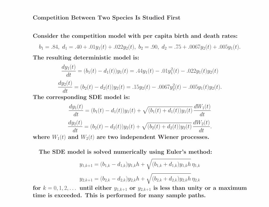
Competition Between Two Species Is Studied First

Consider the competition model with per capita birth and death rates:

b1 = .84, d1 = .40 + .01y1(t) + .022y2(t), b2 = .90, d2 = .75 + .0067y2(t) + .005y1(t).

The resulting deterministic model is:

dy1(t)

dt= (b1(t) − d1(t))y1(t) = .44y1(t) − .01y2

1(t) − .022y1(t)y2(t)

dy2(t)

dt= (b2(t) − d2(t))y2(t) = .15y2(t) − .0067y2

2(t) − .005y1(t)y2(t).

The corresponding SDE model is:

dy1(t)

dt= (b1(t) − d1(t))y1(t) +

√

(b1(t) + d1(t))y1(t)dW1(t)

dt

dy2(t)

dt= (b2(t) − d2(t))y2(t) +

√

(b2(t) + d2(t))y2(t)dW2(t)

dt.

where W1(t) and W2(t) are two independent Wiener processes.

The SDE model is solved numerically using Euler’s method:

y1,k+1 = (b1,k − d1,k)y1,kh +√

(b1,k + d1,k)y1,kh η1,k

y2,k+1 = (b2,k − d2,k)y2,kh +√

(b2,k + d2,k)y2,kh η2,k

for k = 0, 1, 2, . . . until either y1,k+1 or y2,k+1 is less than unity or a maximum

time is exceeded. This is performed for many sample paths.

Calculational Results Illustrate A Difference Between Deterministic And

Stochastic Models

For the deterministic model, the first species always out-competes the sec-

ond species.

For the stochastic model, the second species out-competes the first species

about 44% of the time.

0 20 40 600

5

10

15

Pop. y1

Pop.

y2

Deterministic

0 50 1000

20

40

60

Time t

Pops

. 1 a

nd 2

Deterministic

0 20 400

10

20

30

40

Pop. y1

Pop.

y2

0 10 200

10

20

30

40

Time t

Pops

. 1 a

nd 2

Figure 6: Calculational Results For The Deterministic And Stochastic Models For A Competition System

In The Project, Five Systems Are Studied

Two Competition Systems

A Predator-Prey System

An Epidemic System (SIS)

A System of Your Choice

discrete-time stochastic models, sdes, and numerical methods

Documents