discrete time fourier transform (dtft) - prod … · properties are very similar to the discrete...
TRANSCRIPT

Discrete Time Fourier Transform(DTFT)

Discrete Time Fourier Transform (DTFT)
The DTFT is the Fourier transform of choice for analyzing infinite-length signals and systems
Useful for conceptual, pencil-and-paper work, but not Matlab friendly (infinitely-long vectors)
Properties are very similar to the Discrete Fourier Transform (DFT) with a few caveats
We will derive the DTFT as the limit of the DFT as the signal length N →∞
2

Recall: DFT (Unnormalized)
Analysis (Forward DFT)
• Choose the DFT coefficients X[k] such that the synthesis produces the signal x
• The weight X[k] measures the similarity between x and the harmonic sinusoid sk
• Therefore, X[k] measures the “frequency content” of x at frequency k
Xu[k] =
N−1∑n=0
x[n] e−j2πN kn
Synthesis (Inverse DFT)
• Build up the signal x as a linear combination of harmonic sinusoids sk weighted by the
DFT coefficients X[k]
x[n] =1
N
N−1∑k=0
Xu[k] ej 2πN kn
3

The Centered DFT
Both x[n] and X[k] can be interpreted as periodic with period N , so we will shift the intervals ofinterest in time and frequency to be centered around n, k = 0
−N2≤ n, k ≤ N
2− 1
The modified forward and inverse DFT formulas are
Xu[k] =
N/2−1∑n=−N/2
x[n] e−j2πN kn, −N
2≤ k ≤ N
2− 1
x[n] =1
N
N/2−1∑k=−N/2
Xu[k] ej 2πN kn − N
2≤ n ≤ N
2− 1
4

Recall: DFT Frequencies
Xu[k] =
N/2−1∑n=−N/2
x[n] e−j2πN kn, −N
2≤ k ≤ N
2− 1
Xu[k] measures the similarity between the time signal x and the harmonic sinusoid sk
Therefore, Xu[k] measures the “frequency content” of x at frequency
−π ≤ ωk =2π
Nk < π
−15 −10 −5 0 5 10 150
5
k
|X[k]|
5
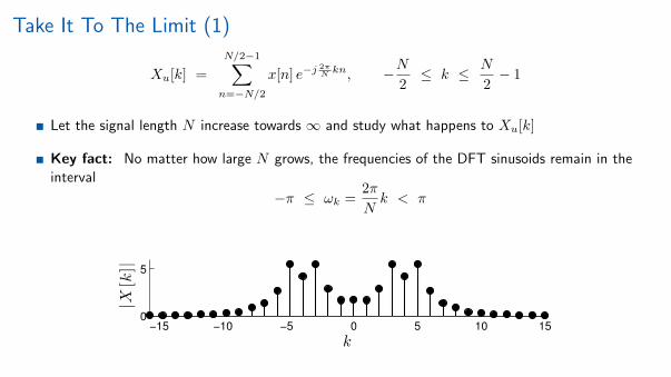
Take It To The Limit (1)
Xu[k] =
N/2−1∑n=−N/2
x[n] e−j2πN kn, −N
2≤ k ≤ N
2− 1
Let the signal length N increase towards ∞ and study what happens to Xu[k]
Key fact: No matter how large N grows, the frequencies of the DFT sinusoids remain in theinterval
−π ≤ ωk =2π
Nk < π
−15 −10 −5 0 5 10 150
5
k
|X[k]|
6

Take It To The Limit (2)Xu[k] =
N/2−1∑n=−N/2
x[n] e−j2πN kn
N time signal x[n] DFT X[k]
32−15 −10 −5 0 5 10 15
−1
0
1
n−15 −10 −5 0 5 10 15
0
5
k
64−30 −20 −10 0 10 20 30
−1
0
1
n−30 −20 −10 0 10 20 30
0
5
k
128−60 −40 −20 0 20 40 60
−1
0
1
n−60 −40 −20 0 20 40 60
0
5
k
256−100 −50 0 50 100
−1
0
1
n−100 −50 0 50 100
0
5
k
7

Discrete Time Fourier Transform (Forward)
As N →∞, the forward DFT converges to a function of the continuous frequency variable ωthat we will call the forward discrete time Fourier transform (DTFT)
N/2−1∑n=−N/2
x[n] e−j2πN kn −→
∞∑n=−∞
x[n] e−jωn = X(ω), − π ≤ ω < π
Recall: Inner product for infinite-length signals
〈x, y〉 =
∞∑n=−∞
x[n] y[n]∗
Analysis interpretation: The value of the DTFT X(ω) at frequency ω measures the similarityof the infinite-length signal x[n] to the infinite-length sinusoid ejωn
8
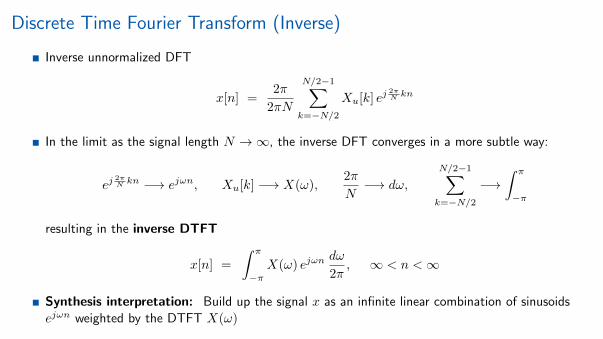
Discrete Time Fourier Transform (Inverse)
Inverse unnormalized DFT
x[n] =2π
2πN
N/2−1∑k=−N/2
Xu[k] ej 2πN kn
In the limit as the signal length N →∞, the inverse DFT converges in a more subtle way:
ej2πN kn −→ ejωn, Xu[k] −→ X(ω),
2π
N−→ dω,
N/2−1∑k=−N/2
−→∫ π
−π
resulting in the inverse DTFT
x[n] =
∫ π
−πX(ω) ejωn
dω
2π, ∞ < n <∞
Synthesis interpretation: Build up the signal x as an infinite linear combination of sinusoidsejωn weighted by the DTFT X(ω)
9
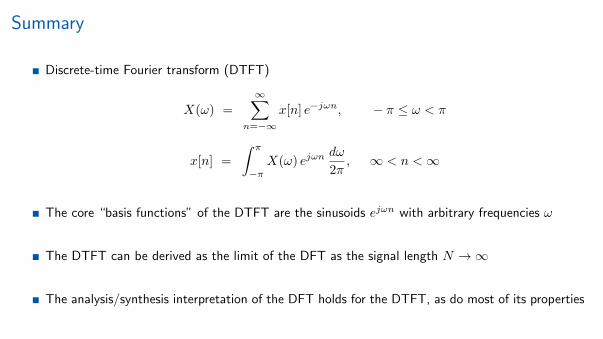
Summary
Discrete-time Fourier transform (DTFT)
X(ω) =
∞∑n=−∞
x[n] e−jωn, − π ≤ ω < π
x[n] =
∫ π
−πX(ω) ejωn
dω
2π, ∞ < n <∞
The core “basis functions” of the DTFT are the sinusoids ejωn with arbitrary frequencies ω
The DTFT can be derived as the limit of the DFT as the signal length N →∞
The analysis/synthesis interpretation of the DFT holds for the DTFT, as do most of its properties
10

Eigenanalysis ofLTI Systems(Infinite-Length Signals)
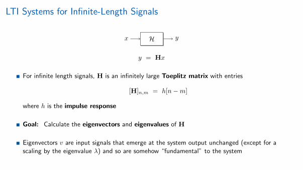
LTI Systems for Infinite-Length Signals
x H y
y = Hx
For infinite length signals, H is an infinitely large Toeplitz matrix with entries
[H]n,m = h[n−m]
where h is the impulse response
Goal: Calculate the eigenvectors and eigenvalues of H
Eigenvectors v are input signals that emerge at the system output unchanged (except for ascaling by the eigenvalue λ) and so are somehow “fundamental” to the system
2

Eigenvectors of LTI Systems
Fact: The eigenvectors of a Toeplitz matrix (LTI system) are the complex sinusoids
sω[n] = ejωn = cos(ωn) + j sin(ωn), −π ≤ ω < π, −∞ < n <∞
−8 −6 −4 −2 0 2 4 6−1
0
1
cos(ωn)
n
−8 −6 −4 −2 0 2 4 6−4
−2
0
2
4
λω cos(ωn)
nsω H λωsω
−8 −6 −4 −2 0 2 4 6−1
0
1
sin(ωn)
n
−8 −6 −4 −2 0 2 4 6−4
−2
0
2
4
λω sin(ωn)
n
3

Sinusoids are Eigenvectors of LTI Systems
sω H λωsω
Prove that harmonic sinusoids are the eigenvectors of LTI systems simply by computing theconvolution with input sω and applying the periodicity of the sinusoids (infinite-length)
sω[n] ∗ h[n] =
∞∑m=−∞
sω[n−m]h[m] =
∞∑m=−∞
ejω(n−m) h[m]
=
∞∑m=−∞
ejωn e−jωm h[m] =
( ∞∑m=−∞
h[m] e−jωm
)ejωn
= λω sω[n] X
4

Eigenvalues of LTI SystemsThe eigenvalue λω ∈ C corresponding to the sinusoid eigenvector sω is called the frequencyresponse at frequency ω since it measures how the system “responds” to sk
λω =
∞∑n=−∞
h[n] e−ωn = 〈h, sω〉 = H(ω) (DTFT of h)
Recall properties of the inner product: λω grows/shrinks as h and sω become more/less similar
−8 −6 −4 −2 0 2 4 6−1
0
1
cos(ωn)
n
−8 −6 −4 −2 0 2 4 6−4
−2
0
2
4
λω cos(ωn)
nsω H λωsω
−8 −6 −4 −2 0 2 4 6−1
0
1
sin(ωn)
n
−8 −6 −4 −2 0 2 4 6−4
−2
0
2
4
λω sin(ωn)
n
5

Eigendecomposition and Diagonalization of an LTI System
x H y
y[n] = x[n] ∗ h[n] =
∞∑m=−∞
h[n−m]x[m]
While we can’t explicitly display the infinitely large matrices involved, we can use the DTFT to“diagonalize” an LTI system
Taking the DTFTs of x and h
X(ω) =
∞∑m=−∞
x[n] e−ωn, H(ω) =
∞∑m=−∞
h[n] e−ωn
we have thatY (ω) = X(ω)H(ω)
and then
y[n] =
∫ π
−πY (ω) ejωn
dω
2π
6
Summary
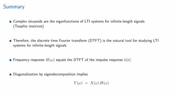
Complex sinusoids are the eigenfunctions of LTI systems for infinite-length signals(Toeplitz matrices)
Therefore, the discrete time Fourier transform (DTFT) is the natural tool for studying LTIsystems for infinite-length signals
Frequency response H(ω) equals the DTFT of the impulse response h[n]
Diagonalization by eigendecomposition implies
Y (ω) = X(ω)H(ω)
7

Discrete Time Fourier TransformExamples

Discrete Time Fourier Transform
X(ω) =
∞∑n=−∞
x[n] e−jωn, − π ≤ ω < π
x[n] =
∫ π
−πX(ω) ejωn
dω
2π, ∞ < n <∞
The Fourier transform of choice for analyzing infinite-length signals and systems
Useful for conceptual, pencil-and-paper work, but not Matlab friendly (infinitely-long vectors)
2

DTFT of the Unit Pulse (1)
Compute the DTFT of the symmetrical unit pulse p[n] =
{1 −M ≤ n ≤M0 otherwise
Note: Duration Dx = 2M + 1 samples
Example for M = 3
−15 −10 −5 0 5 10 150
0.5
1
p[n ]
n
Forward DTFT
P (ω) =
∞∑n=−∞
p[n] e−jωn =
M∑n=−M
e−jωn . . .
3

DTFT of the Unit Pulse (2)
Apply the finite geometric series formula
P (ω) =
∞∑n=−∞
p[n] e−jωn =
M∑n=−M
e−jωn =
M∑n=−M
(e−jω
)n=
ejωM − e−jω(M+1)
1− e−jω
This is an answer but it is not simplified enough to make sense, so we continue simplifying
P (ω) =ejωM − e−jω(M+1)
1− e−jω =e−jω/2
(ejω
2M+12 − e−jω 2M+1
2
)e−jω/2
(ejω/2 − e−jω/2
)=
2j sin(ω 2M+1
2
)2j sin
(ω2
)
4

DTFT of the Unit Pulse (3)
Simplified DTFT of the unit pulse of duration Dx = 2M + 1 samples
P (ω) =sin(2M+1
2 ω)
sin(ω2
)This is called the Dirichlet kernel or “digital sinc”
• It has a shape reminiscent of the classical sinx/x sinc function, but it is 2π-periodic
If p[n] is interpreted as the impulse response of the moving average system, then P (ω) is thefrequency response (eigenvalues) (low-pass filter)
−15 −10 −5 0 5 10 150
0.5
1
p[n ]
n−π −π/2 0 π/2 π
−0.5
0
0.5
1
ω
P (ω)
5

DTFT of a One-Sided Exponential
Recall the impulse response of the recursive average system: h[n] = αn u[n], |α| < 1
Compute the frequency response H(ω)
Forward DTFT
H(ω) =
∞∑n=−∞
h[n] e−jωn =
∞∑n=0
αn e−jωn =
∞∑n=0
(α e−jω)n =1
1− α e−jω
Recursive system with α = 0.8 is a low-pass filter
−8 −6 −4 −2 0 2 4 6 80
0.5
1
h[n ] = αn u[n ], α = 0.8
n−π −π/2 0 π/2 π0
2
4
6
ω
|H (ω)|
6

Impulse Response of the Ideal Lowpass Filter (1)
The frequency response H(ω) of the ideal low-pass filter passes low frequencies (near ω = 0)but blocks high frequencies (near ω = ±π)
H(ω) =
{1 −ωc ≤ ω ≤ ωc0 otherwise
Compute the impulse response h[n] given this H(ω)
Apply the inverse DTFT
h[n] =
∫ π
−πH(ω) ejωn
dω
2π=
∫ ωc
−ωc
ejωndω
2π=
ejωn
jn
∣∣∣∣ωc
−ωc
=ejωcn − e−jωcn
jn= 2ωc
sin(ωcn)
ωcn
7
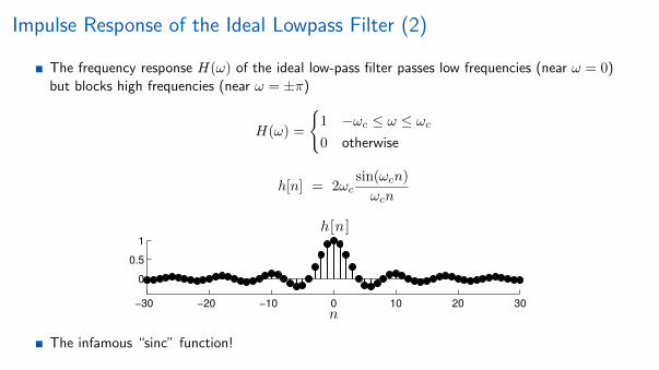
Impulse Response of the Ideal Lowpass Filter (2)
The frequency response H(ω) of the ideal low-pass filter passes low frequencies (near ω = 0)but blocks high frequencies (near ω = ±π)
H(ω) =
{1 −ωc ≤ ω ≤ ωc0 otherwise
h[n] = 2ωcsin(ωcn)
ωcn
−30 −20 −10 0 10 20 30
0
0.5
1
h[n ]
n
The infamous “sinc” function!
8

Summary
DTFT of a rectangular pulse is a Dirichlet kernel
DTFT of a one-sided exponential is a low-frequency bump
Inverse DTFT of the ideal lowpass filter is a sinc function
Work some examples on your own!
9

Discrete Time Fourier Transformof a Sinusoid

Discrete Fourier Transform (DFT) of a Harmonic Sinusoid
Thanks to the orthogonality of the length-N harmonic sinusoids, it is easy to calculate the DFTof the harmonic sinusoid x[n] = sl[n] = ej
2πN ln/
√N
X[k] =
N−1∑n=0
sl[n]e−j
2πN kn
√N
= 〈sl, sk〉 = δ[k − l]
0 5 10 15 20 25 30−0.2
0
0.2
s4[n]
n0 5 10 15 20 25 30
0
0.5
1
S4[k ]
n
So what is the DTFT of the infinite length sinusoid ejω0n?
2
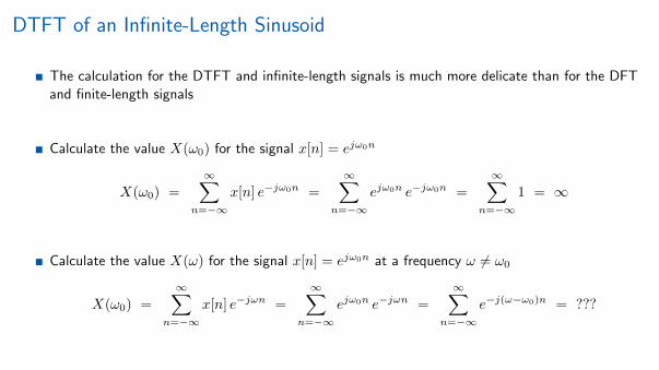
DTFT of an Infinite-Length Sinusoid
The calculation for the DTFT and infinite-length signals is much more delicate than for the DFTand finite-length signals
Calculate the value X(ω0) for the signal x[n] = ejω0n
X(ω0) =
∞∑n=−∞
x[n] e−jω0n =
∞∑n=−∞
ejω0n e−jω0n =
∞∑n=−∞
1 = ∞
Calculate the value X(ω) for the signal x[n] = ejω0n at a frequency ω 6= ω0
X(ω0) =∞∑
n=−∞x[n] e−jωn =
∞∑n=−∞
ejω0n e−jωn =∞∑
n=−∞e−j(ω−ω0)n = ???
3
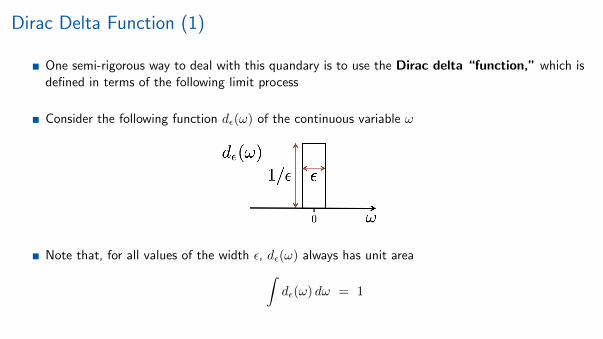
Dirac Delta Function (1)
One semi-rigorous way to deal with this quandary is to use the Dirac delta “function,” which isdefined in terms of the following limit process
Consider the following function dε(ω) of the continuous variable ω
Note that, for all values of the width ε, dε(ω) always has unit area∫dε(ω) dω = 1
4
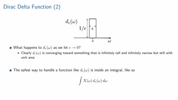
Dirac Delta Function (2)
What happens to dε(ω) as we let ε→ 0?
• Clearly dε(ω) is converging toward something that is infinitely tall and infinitely narrow but still with
unit area
The safest way to handle a function like dε(ω) is inside an integral, like so∫X(ω) dε(ω) dω
5

Dirac Delta Function (3)
As ε→ 0, it seems reasonable that∫X(ω) dε(ω) dω
ε→0−→ X(0)
and ∫X(ω) dε(ω − ω0) dω
ε→0−→ X(ω0)
So we can think of dε(ω) as a kind of “sampler” that picks out values of functions from inside anintegral
We describe the results of this limiting process (as ε→ 0) as the Dirac delta “function” δ(ω)
6

Dirac Delta Function (4)
Dirac delta “function” δ(ω)
We write ∫X(ω) δ(ω) dω = X(0)
and ∫X(ω) δ(ω − ω0) dω = X(ω0)
Remarks and caveats
• Do not confuse the Dirac delta “function” with the nicely behaved discrete delta function δ[n]• The Dirac has lots of “delta,” but it is not really a “function” in the normal sense (it can be made
more rigorous using the theory of generalized functions)• Colloquially, engineers will describe the Dirac delta as “infinitely tall and infinitely narrow”
7
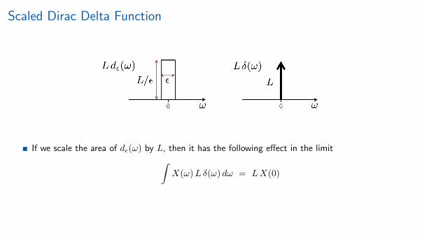
Scaled Dirac Delta Function
If we scale the area of dε(ω) by L, then it has the following effect in the limit∫X(ω)Lδ(ω) dω = LX(0)
8

And Now Back to Our Regularly Scheduled Program . . .
Back to determining the DTFT of an infinite length sinusoid
Rather than computing the DTFT of a sinusoid using the forward DTFT, we will show that aninfinite-length sinusoid is the inverse DTFT of the scaled Dirac delta function 2πδ(ω − ω0)∫ π
−π2πδ(ω − ω0) e
jωn dω
2π= ejω0n
Thus we have the (rather bizarre) DTFT pair
ejω0n DTFT←→ 2π δ(ω − ω0)
9

DTFT of Real-Valued Sinusoids
Since
cos(ω0n) =1
2
(ejω0n + e−jω0n
)we can calculate its DTFT as
cos(ω0n)DTFT←→ π δ(ω − ω0) + π δ(ω + ω0)
Since
sin(ω0n) =1
2j
(ejω0n − e−jω0n
)we can calculate its DTFT as
sin(ω0n)DTFT←→ π
jδ(ω − ω0) +
π
jδ(ω + ω0)
10

Summary
The DTFT would be of limited utility if we could not compute the transform of an infinite-lengthsinusoid
Hence, the Dirac delta “function” (or something else) is a necessary evil
The Dirac delta has infinite energy (2-norm); but then again so does an infinite-length sinusoid
11

Discrete Time Fourier TransformProperties

Recall: Discrete-Time Fourier Transform (DTFT)
Forward DTFT (Analysis)
X(ω) =
∞∑n=−∞
x[n] e−jωn, − π ≤ ω < π
Inverse DTFT (Synthesis)
x[n] =
∫ π
−πX(ω) ejωn
dω
2π, ∞ < n <∞
DTFT pair
x[n]DTFT←→ X(ω)
2

The DTFT is Periodic
We defined the DTFT over an interval of ω of length 2π, but it can also be interpreted asperiodic with period 2π
X(ω) = X(ω + 2πk), k ∈ Z
Proof
X(ω + 2πk) =
∞∑n=−∞
x[n] e−j(ω+2πk)n =
∞∑n=−∞
x[n] e−jωn e−j2πkn = X(ω) X
−3π −2π −π 0 π 2π 3π−0.5
0
0.5
1
ω
X (ω)
3

DTFT Frequencies
X(ω) =
∞∑n=−∞
x[n] e−jωn, − π ≤ ω < π
X(ω) measures the similarity between the time signal x and and a sinusoid ejωn of frequency ω
Therefore, X(ω) measures the “frequency content” of x at frequency ω
−π −π/2 0 π/2 π−0.5
0
0.5
1
ω
X (ω)
4

DFT Frequencies and Periodicity
Periodicity of DFT means we can treat frequencies mod 2π
X(ω) measures the “frequency content” of x at frequency (ω)2π
−3π −2π −π 0 π 2π 3π−0.5
0
0.5
1
ω
X (ω)
5
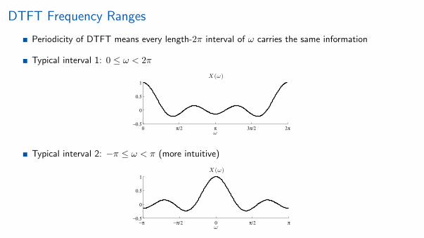
DTFT Frequency Ranges
Periodicity of DTFT means every length-2π interval of ω carries the same information
Typical interval 1: 0 ≤ ω < 2π
0 π/2 π 3π/2 2π−0.5
0
0.5
1
ω
X (ω)
Typical interval 2: −π ≤ ω < π (more intuitive)
−π −π/2 0 π/2 π−0.5
0
0.5
1
ω
X (ω)
6
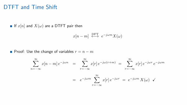
DTFT and Time Shift
If x[n] and X(ω) are a DTFT pair then
x[n−m]DFT←→ e−jωmX(ω)
Proof: Use the change of variables r = n−m∞∑
n=−∞x[n−m] e−jωn =
∞∑r=−∞
x[r] e−jω(r+m) =
∞∑r=−∞
x[r] e−jωr e−jωm
= e−jωm∞∑
r=−∞x[r] e−jωr = e−jωmX(ω) X
7
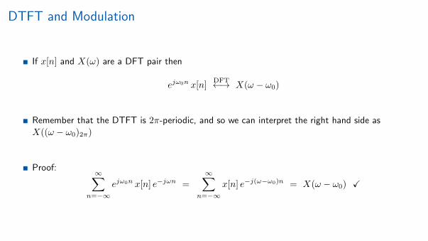
DTFT and Modulation
If x[n] and X(ω) are a DFT pair then
ejω0n x[n]DFT←→ X(ω − ω0)
Remember that the DTFT is 2π-periodic, and so we can interpret the right hand side asX((ω − ω0)2π)
Proof:∞∑
n=−∞ejω0n x[n] e−jωn =
∞∑n=−∞
x[n] e−j(ω−ω0)n = X(ω − ω0) X
8

DTFT and Convolution
x h y
y[n] = x[n] ∗ h[n] =
∞∑m=−∞
h[n−m]x[m]
Ifx[n]
DTFT←→ X(ω), h[n]DTFT←→ H(ω), y[n]
DTFT←→ Y (ω)
thenY (ω) = H(ω)X(ω)
Convolution in the time domain = multiplication in the frequency domain
9

The DTFT is Linear
It is trivial to show that if
x1[n]DTFT←→ X1(ω) x2[n]
DTFT←→ X2(ω)
then
α1x1[n] + α2x[2]DFT←→ α1X1(ω) + α2X2(ω)
10

DTFT Symmetry Properties
The sinusoids ejωn of the DTFT have symmetry properties:
Re(ejωn
)= cos (ωn) (even function)
Im(ejωn
)= sin (ωn) (odd function)
These induce corresponding symmetry properties on X(ω) around the frequency ω = 0
Even signal/DFTx[n] = x[−n], X(ω) = X(−ω)
Odd signal/DFTx[n] = −x[−n], X(ω) = −X(−ω)
Proofs of the symmetry properties are identical to the DFT case; omitted here
11

DFT Symmetry Properties Table
x[n] X(ω) Re(X(ω)) Im(X(ω)) |X(ω)| ∠X(ω)
real X(−ω) = X(ω)∗ even odd even odd
real & even real & even even zero even
real & odd imaginary & odd zero odd even
imaginary X(−ω) = −X(ω)∗ odd even even odd
imaginary & even imaginary & even zero even even
imaginary & odd imaginary & odd odd zero even
12
Summary
DTFT is periodic with period 2π
Convolution in time becomes multiplication in frequency
DTFT has useful symmetry properties
13

Acknowledgements
c© 2014 Richard Baraniuk, All Rights Reserved
2