Theoretical Computer Sceince, to appear

Discrete Random Variables Over Domains

Michael Mislove 1

Department of Mathematics

Tulane University

New Orleans, LA 70118

Abstract

In this paper we initiate the study of discrete random variables over domains. Ourwork is inspired by work of Daniele Varacca, who devised indexed valuations asmodels of probabilistic computation within domain theory. Our approach relieson new results about commutative monoids defined on domains that also allowactions of the non-negative reals. Using our approach, we define two such familiesof real domain monoids, one of which allows us to recapture Varacca’s constructionof the Plotkin indexed valuations over a domain. Each of these families leads tothe construction of a family of discrete random variables over domains, the secondof which forms the object level of a continuous endofunctor on the categories RB

(domains that are retracts of bifinite domains), and on FS (domains where theidentity map is the directed supremum of deflations finitely separated from theidentity). The significance of this last result lies in the fact that there is no knowncategory of continuous domains that is closed under the probabilistic power domain,which forms the standard approach to modeling probabilistic choice over domains.The fact that RB and FS are Cartesian closed and also are closed under a powerdomain of discrete random variables means we can now model, e.g., the untypedlambda calculus extended with a probabilistic choice operator, implemented viarandom variables.

1 Introduction

Domain theory, perhaps the most widely used method for assigning deno-tational meanings to programming languages, has recently seen its influencebroaden to other areas of computation and mathematics. It provides a broadrange of constructors for modeling data types, nondeterminism, functionalprogramming, and several other constructs needed in semantics. Domain the-ory also admits a number of Cartesian closed categories, the fundamental

1 This work supported by the US National Science Foundation and the US Office of NavalResearch

Preprint submitted to Elsevier Preprint 17 August 2006

Mislove

objects needed to model the lambda calculus. Even probabilistic computationadmits a model in the theory, although truth to tell, this particular construc-tor has proven to be very difficult to unravel. Of particular interest is thequestion

Is there a Cartesian closed category of domainsthat is closed under the probabilistic power domain?

There have been many attempts to resolve this, but the most we know to dateis contained in [12], where it is shown that the probabilistic power domain ofa finite tree is in RB, that the probabilistic power domain of a finite reversedtree is in FS, and that RB is closed under the probabilistic power domain ifthe probabilistic power domain of every finite poset is in RB. But, other thanfinite trees, the only finite posets whose probabilistic power domain is knownto be in RB is the class of flat posets, whose probabilistic power domains arebounded complete (the continuous analogs of Scott domains).

We do not contribute to settling this question here, but we do provide analternative construction—what we call the power domain of discrete ×-randomvariables, which we show defines a continuous endofunctor on the category RB,as well as on FS and on CDOM, the category of coherent domains.

Objects in RB are retracts of bifinite domains, those that can be expressedas bilimits of finite posets under embedding–projection pairs. This categoryis Cartesian closed, and it also is closed under the various power domains fornondeterminism [7]. With the addition of a mechanism to model probabilisticchoice, RB provides virtually all the tools required to support semantic mod-eling. Furthermore, playing off results of Varacca [23,24], we show that theformation of the power domain of discrete ×-random variables over RB yieldsa monad that enjoys a distributive law with respect to each of the powerdomain monads, and this in turn implies that each of these power domainmonads lifts to a monad on the category RB that are also algebras for thediscrete ×-random variable power domain monad. These laws are enumer-ated in Definition 4.8. In short, we can now form domain-theoretic modelsof computation that respect the laws of discrete ×-random variables as wellas any of the laws we choose for nondeterminism: angelic, demonic or convexchoice.

The outline of the rest of the paper is as follows. In the next section weprovide some background about domains and about the constructions we need.We then review briefly a construction by Varacca [24] which inspired our work,and that Varacca calls the Plotkin indexed valuations. In the following section,we investigate bag domains—domain-theoretic models for multisets, and wealso explore the structure of bag domains that also admit an action of the non-negative reals. We single out two such constructs, which are distinguished byhow the least element acts. In the first, ⊥ is the identity of the monoid, as wellas being the image of 0 under the action of R≥0. We define a functor whichproduces the initial such algebra over a bag domain, and this in turn is what we

2

Mislove

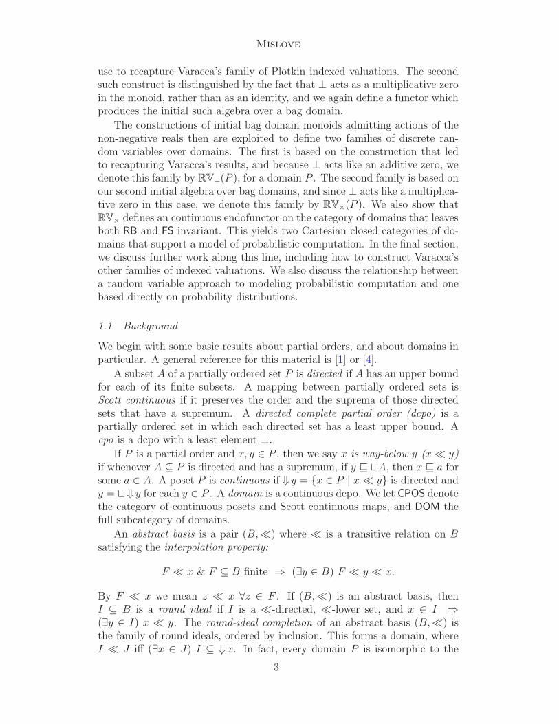
use to recapture Varacca’s family of Plotkin indexed valuations. The secondsuch construct is distinguished by the fact that ⊥ acts as a multiplicative zeroin the monoid, rather than as an identity, and we again define a functor whichproduces the initial such algebra over a bag domain.

The constructions of initial bag domain monoids admitting actions of thenon-negative reals then are exploited to define two families of discrete ran-dom variables over domains. The first is based on the construction that ledto recapturing Varacca’s results, and because ⊥ acts like an additive zero, wedenote this family by RV+(P ), for a domain P . The second family is based onour second initial algebra over bag domains, and since ⊥ acts like a multiplica-tive zero in this case, we denote this family by RV×(P ). We also show thatRV× defines an continuous endofunctor on the category of domains that leavesboth RB and FS invariant. This yields two Cartesian closed categories of do-mains that support a model of probabilistic computation. In the final section,we discuss further work along this line, including how to construct Varacca’sother families of indexed valuations. We also discuss the relationship betweena random variable approach to modeling probabilistic computation and onebased directly on probability distributions.

1.1 Background

We begin with some basic results about partial orders, and about domains inparticular. A general reference for this material is [1] or [4].

A subset A of a partially ordered set P is directed if A has an upper boundfor each of its finite subsets. A mapping between partially ordered sets isScott continuous if it preserves the order and the suprema of those directedsets that have a supremum. A directed complete partial order (dcpo) is apartially ordered set in which each directed set has a least upper bound. Acpo is a dcpo with a least element ⊥.

If P is a partial order and x, y ∈ P , then we say x is way-below y (x≪ y)if whenever A ⊆ P is directed and has a supremum, if y ⊑ ⊔A, then x ⊑ a forsome a ∈ A. A poset P is continuous if ⇓ y = {x ∈ P | x ≪ y} is directed andy = ⊔⇓ y for each y ∈ P . A domain is a continuous dcpo. We let CPOS denotethe category of continuous posets and Scott continuous maps, and DOM thefull subcategory of domains.

An abstract basis is a pair (B,≪) where ≪ is a transitive relation on Bsatisfying the interpolation property:

F ≪ x & F ⊆ B finite ⇒ (∃y ∈ B) F ≪ y ≪ x.

By F ≪ x we mean z ≪ x ∀z ∈ F . If (B,≪) is an abstract basis, thenI ⊆ B is a round ideal if I is a ≪-directed, ≪-lower set, and x ∈ I ⇒(∃y ∈ I) x ≪ y. The round-ideal completion of an abstract basis (B,≪) isthe family of round ideals, ordered by inclusion. This forms a domain, whereI ≪ J iff (∃x ∈ J) I ⊆ ⇓ x. In fact, every domain P is isomorphic to the

3

Mislove

round-ideal completion of an abstract basis, namely P is isomorphic to theround ideal completion of (P,≪) under the mapping sending a point x to ⇓ x,whose inverse is the mapping that sends a round ideal to its supremum.

One of the fundamental results about dcpos is that the family of Scottcontinuous maps between two dcpos is another dcpo in the pointwise order.Since it’s easy to show that the finite product of a family of continuous posetsis another such, and the one-point poset is a terminal object, a central questionis under what conditions is the family of Scott continuous selfmaps [D → E]between domains also continuous, i.e., which categories of dcpos and Scottcontinuous maps are Cartesian closed? This is true of DCPO, the categoryof dcpos and Scott continuous maps, but not of DOM. Still, there are severalfull subcategories of DOM that are Cartesian closed. Among the notable suchcategories are the following: 2

BCD Bounded complete domains, in which every subset having an upper boundhas a least upper bound; equivalently, every non-empty subset has a greatestlower bound.

RB Domains which are retracts of bifinite domains, themselves bilimits of fam-ilies of finite posets under embedding-projection maps; these are pairs ofScott continuous mappings e : P → Q and p : Q → P satisfying p ◦ e = 1P

and e ◦ p ≤ 1Q.

FS Domains D satisfying the property that the identity map is the directedsupremum of Scott-continuous selfmaps f : D → D each finitely separatedfrom the identity: i.e., for each f there is a finite subset Mf ⊆ D with theproperty that, for each x ∈ D, there is some m ∈Mf with f(x) ≤ m ≤ x.

Actually, BCD is a full subcategory of RB, which in turn is a full subcategoryof FS, and FS is a maximal ccc of domains. An interesting (some might sayfrustrating) open question is whether RB and FS are equal. The objects in allof these categories are coherent, 3 but the category CDOM of coherent domainsand Scott continuous maps is not a ccc.

We also recall some facts about categories. A monad or triple on a categoryA is a a 3-tuple 〈T, µ, η〉 where T : A → A is an endofunctor, and µ : T 2 .

−→ Tand η : 1A

.−→ T are natural transformations satisfying the laws:

µ ◦ Tµ = µ ◦ µT and µ ◦ ηT = T = µ ◦ Tη.

Equivalently, if F : A → B is left adjoint to G : B → A with unit η : 1A

·−→ GF

and counit ǫ : FG·

−→ 1B, then 〈GF,GǫF, η〉 forms a monad on A, and everymonad arises in this fashion.

If 〈T, µ, η〉 is a monad, then a T -algebra is a pair (a, h), where a ∈ A andh : Ta→ a is an A-morphism satisfying h ◦ ηa = 1a and h ◦ Th = h ◦ µa.

For example, domain theory provides three models for nondeterminism, thelower power domain PL,which assigns to a domain the family of Scott-closed

2 See [1] for details about these categories.3 A domain is coherent if its Lawson topology is compact; cf. [1]

4

Mislove

lower sets with union as the semilattice operation, the upper power domain,PU which assigns to a domain the family of Scott-compact upper sets withunion as the operation, but with reverse inclusion as the order, and the convexpower domain, PC , which assigns to a (coherent) domain the family of sets thatcan be expressed as the intersection of a Scott-closed lower set and a Scott-compact upper set, with the Egli-Milner order, where the “sum” of sets is thesmallest such set containing their union (cf. [1] for details here). Each of thesedefines a monad on DCPO (cf. [7]), whose algebras are ordered semilattices;another example is the probabilistic power domain V whose algebras satisfyequations that characterize the probability measures over P (cf. [10]).

One goal of domain theory is to provide a setting in which all of the con-structors needed to model a given programming language can be combined. Ifthe aim is to model both nondeterminism and probabilistic choice, then oneneeds to combine the appropriate nondeterminism monad with the probabilis-tic power domain monad, so that the laws of each constructor are preserved inthe resulting model. This is the function of a distributive law, which is a nat-ural transformation d : ST

.−→ TS between monads S and T on A satisfying

several identities—cf. [2]. The significance of distributive laws is the followingtheorem of Beck:

Theorem 1.1 (Beck [2]) Let (T, ηT , µT ) and (S, ηS, µS) be monads on thecategory A. Then there is a one-to-one correspondence between

(i) Distributive laws d : ST.

−→ TS;

(ii) Multiplications µ : TSTS.

−→ TS, satisfying• (TS, ηTηS, µ) is a monad;• the natural transformations ηTS : S

.−→ TS and TηS : T

.−→ TS are

monad morphisms;• the following middle unit law holds:

TSTηSηT S

//

IdTS

&&L

L

L

L

L

L

L

L

L

L

L

L

L

L

TSTS

µ

��

TS

(iii) Liftings T of the monad T to AS, the category of S-algebras in A. 2

So, one way to know that the combination of the probabilistic power do-main and one of the power domains for nondeterminism provides a modelsatisfying all the needed laws would be to show there is a distributive law ofone of these monads over the probabilistic power domain monad. Unfortu-nately, it was shown by Plotkin and Varacca [23] that there is no distributivelaw of V over PX , or of PX over V for any of the nondeterminism monads PX .This led to the work we report on next.

5

Mislove

2 Indexed Valuations

We now recall some of the work of Varacca [24] that was motivated by prob-lems associated with trying to support both nondeterminism and probabilisticchoice within the same model. Once it was shown that there is no distributivelaw between V and any of the nondeterminism monads, Varacca consideredthe simpler situation of sets, where the model of nondeterminism is the powerset monad, and, in the finite case, the probabilistic monad is the family ofsimple measures on the set. A theorem of Gautam shows why the distributivelaw doesn’t hold in this setting:

Theorem 2.1 (Gautam [3]) A necessary and sufficient condition for anequational theory to extend from a model X to its power set is that everylaw of the theory mentions each variable at most once on each side of theequation. 2

Since finite posets are domains, this implies that, even ifX is a probabilisticalgebra, the operations on X cannot be extended to P(X) to satisfy thesame laws. In fact, both the nondeterminism monad over a set X and theprobabilistic monad over X violate the conditions of the theorem. For thenondeterminism monad, it is the law x ⊕ x = x, while for the probabilisticmonad, it is the law pA⊕(1−p)A = A. 4 Then Varacca realized that weakeningone of the laws of probabilistic choice could result in a monad that enjoys adistributive law with respect to a monad for nondeterminism. For 0 < p < 1and A a domain element,Varacca weakened the law pA + (1 − p)A = A inthree ways:

pA+ (1 − p)A ⊒ A, (1)

pA+ (1 − p)A ⊑ A, (2)

pA+ (1 − p)A and A not necessarily related by order. (3)

He called the monad he constructed satisfying (1) the Hoare indexed valua-tions, the one satisfying (2) the Smyth indexed valuations and the one satisfy-ing (3), the Plotkin indexed valuations. We exploit this last construction—theso-called Plotkin indexed valuations over a domain—in the construction of apower domain of discrete random variables.

2.1 Plotkin Indexed Valuations

Definition 2.2 An indexed valuation over the poset P is a tuple (ri, pi)i∈I

where I is an index set, 5 each ri ≥ 0 is a non-negative real number andpi ∈ P for each i ∈ I.

4 The operator pA ⊕ (1 − p)A models probabilistic choice where the left branch is chosenwith probability 0 ≤ p ≤ 1 and the right branch is chosen with probability 1 − p.5 For our discussion, we can assume I is always finite.

6

Mislove

Two indexed valuations satisfy (ri, pi)I ≃1 (sj , qj)J if |I| = |J | and thereis a permutation φ ∈ S(|I|) 6 with rφ(i) = si and pφ(i) = qi for each i.

If I ′ = {i ∈ I | ri 6= 0} and similarly for J , then (ri, pi)I ≃ (sj , qj)J if(ri, pi)I′ ≃1 (sj , qj)J ′ . Then, ≃ is an equivalence relation on indexed valua-tions, and we let 〈ri, pi〉I denote the equivalence class of the indexed valuation(ri, pi)I modulo ≃.

Next, let R≥0 denote the extended non-negative real numbers, with theusual order. Then given a domain P , Varacca defines a relation ≪IVP

on thefamily {〈ri, pi〉I | ri ∈ R≥0 & pi ∈ P} of indexed valuations over P by

〈ri, pi〉I ≪IVP〈sj, qj〉J iff (|I| = |J |) & (∃φ ∈ S(|I|)) (4)

ri ≪ sφ(i) & pi ≪P qφ(i) (∀i ∈ I).6

This forms an abstract basis whose round ideal completion is the family ofPlotkin indexed valuations over P . We denote this domain by IVP (P ).

We also can “add” indexed valuations 〈ri, pi〉I and 〈sj , qj〉J by

〈ri, xi〉i∈I ⊕ 〈sj, yj〉j∈J = 〈tk, zk〉k∈K

where K = I·

∪ J and

(tk, zk) =

{(ri, xi) if k = i ∈ I

(sj, yj) if k = j ∈ J.

This operation of concatenating tuples and taking the equivalence class of the

resulting I·

∪ J-tuple forms a continuous operation on indexed valuations thatis commutative, by construction. We let R≥0 act on 〈ri, pi〉I by r · 〈ri, pi〉I =〈r · ri, pi〉I . Varacca’s main result for the family of Plotkin indexed valuationscan be summarized as follows:

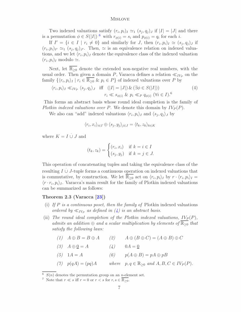
Theorem 2.3 (Varacca [23])

(i) If P is a continuous poset, then the family of Plotkin indexed valuationsordered by ≪IVP

as defined in (4) is an abstract basis.

(ii) The round ideal completion of the Plotkin indexed valuations, IVP (P ),admits an addition ⊕ and a scalar multiplication by elements of R≥0 thatsatisfy the following laws:

(1) A⊕B = B ⊕ A (2) A⊕ (B ⊕ C) = (A⊕ B) ⊕ C

(3) A⊕ 0 = A (4) 0A = 0

(5) 1A = A (6) p(A⊕ B) = pA⊕ pB

(7) p(qA) = (pq)A where p, q ∈ R≥0 and A,B,C ∈ IVP (P ).

6 S(n) denotes the permutation group on an n-element set.7 Note that r ≪ s iff r = 0 or r < s for r, s ∈ R≥0.

7

Mislove

(iii) IVP defines the object level of an endofunctor which is monadic overDOM, and that satisfies a distributive law with respect to each of thepower domain monads. 2

A coherent domain is one whose Lawson topology is compact; it is a stan-dard result of domain theory is that the Plotkin power domain applied toa coherent domain yields another such (cf. [1] for details). A corollary ofTheorem 2.3 is that the composition PP ◦ IVP defines a monad on CDOM,the category of coherent domains, whose algebras satisfy the laws listed inTheorem 2.3(i) and the laws of the Plotkin power domain:

(i) X + Y = Y +X

(ii) X +X = X

(iii) X + (Y + Z) = (X + Y ) + Z

In other words, PP (IVP (P )) is the initial domain semilattice algebra over Pthat also satisfies the laws listed in Theorem 2.3(ii).

3 Bag domains

In this section we develop some results that are fundamental for our mainconstruction. More details about these results are contained in [17]. The ear-liest comments in the literature about bag domains—domains whose elementsare bags or multisets from an underlying domain, are in [20] where Exercise103 discusses them; Poigne [21] also comments on the existence of free bagdomains. But the first paper devoted to bag domains is apparently [6], wherea topological approach to their construction is investigated. There is the workof Vickers [25] and of Johnstone [8,9], but these works were inspired by prob-lems in database theory, and the focus is on abstract categorical construction,not on domains as we consider them. To be sure, we also are interested incategorical aspects, but our aim is more in the spirit of [6], which includesanalyzing the internal structure of these objects. Our results also allow us tocapture the constructions of Varacca [23] more concretely. We begin with asimple result about posets:

Definition 3.1 Let P be a poset and let n ∈ N. For φ ∈ S(n), define amapping

φ : P n → P n by φ(d)i = dφ−1(i). (5)

Then φ permutes the components of d according to φ’s permutation of theindices i = 1, . . . , n. Next, define a preorder �n on P n by

d �n e iff (∃φ ∈ S(n)) φ(d) ≤ e iff (∃φ ∈ S(n)) dφ−1(i) ≤ ei (∀i = 1 . . . , n).(6)

Finally, we define the equivalence relation ≡n on P n by

≡n = �n ∩ �n, (7)

8

Mislove

and we note that (P n/≡n,⊑n) is a partial order. We denote by [d] the imageof d ∈ P n in P n/≡n.

Lemma 3.2 Let P be a poset, let n ∈ N, and let d, e ∈ P n. Then the followingare equivalent:

(i) d ⊑n e,

(ii) ↑{φ(d) | φ ∈ S(n)} ⊇ ↑{φ(e) | φ ∈ S(n)}.

Proof. For (i) implies (ii), we note that, if φ ∈ S(n) satisfies dφ−1(i) ≤ ei, thendi ≤ eφ(i) for each i = 1, . . . , n, so φ−1(e) ∈ ↑ d, and then ψ(e) ∈ ↑{(φ(d) | φ ∈S(n)} for each ψ ∈ S(n) by composing permutations, from which (ii) follows.Conversely, (ii) implies (i) is clear. 2

We also need a classic result due to M.-E. Rudin (cf. Lemma III-3.3 of[4].

Lemma 3.3 (Rudin) Let P be a poset and let {↑Fi | i ∈ I} be a filter basisof non-empty, finitely-generated upper sets. Then there is a directed subsetA ⊆ ∪iFi with A ∩ Fi 6= ∅ for all i ∈ I. 2

Next, let P be a dcpo and let n > 0. We can apply the lemma above toderive the following:

Proposition 3.4 Let P be a dcpo, and let n > 0.

• If A ⊆ P n/≡n is directed, then there is a directed subset B ⊆⋃

[a]∈A{φ(a) |

φ ∈ S(n)} satisfying

↑{φ(⊔B) | φ ∈ S(n)} =⋂

a∈A

↑{φ(a) | φ ∈ S(n)} and [⊔B] = ⊔A. (8)

• In particular, (P n/≡n,⊑) is a dcpo, and the mapping x 7→ [x] : P n → P n/≡n

is Scott continuous.

Proof. If A ⊆ P n/≡n is directed, then Lemma 3.2 implies that {∪φ∈S(n) ↑φ(a) |[a] ∈ A} is a filter basis of finitely generated upper sets, and so by Lemma 3.3there is a directed set B ⊆

⋃[a]∈A{φ(a) | φ ∈ S(n)} with B ∩ {φ(a) | φ ∈

S(n)} 6= ∅ for each [a] ∈ A. Since B ⊆ P n is directed, we have x = ⊔B exists.If [a] ∈ A, then B ∩{φ(a) | φ ∈ S(n)} 6= ∅ means there is some φ ∈ S(n) withφ(a) ∈ B, so φ(a) ≤ x by Lemma 3.2. Hence [a] ⊑ [x] for each [a] ∈ A, so [x]is an upper bound for A.

We also note that, since ⊔B = x,

⋂

b∈B

↑{φ(b) | φ ∈ S(n)} = ↑{φ(x) | φ ∈ S(n)}.

Indeed, the right hand side is clearly contained in the left hand side sinceb ≤ x for all b ∈ B. On the other hand, if y is in the left hand side, then b ⊑ yfor each b ∈ B. Now, since S(n) is finite, there is some φ0 ∈ S(n) and somecofinal subset B′ ⊆ B with φ0(b) ≤ y for each b ∈ B′. But then ⊔B′ = ⊔B,

9

Mislove

and so ⊔{φ0(b) | b ∈ B′} = φ0(x), from which we conclude that φ0(x) ≤ y.Thus y is in the right hand side, so the sets are equal.

Now, if y ∈ P n satisfies [a] ⊑ [y] for each [a] ∈ A, then since B ⊆⋃[a]∈A{φ(a) | φ ∈ S(n)}, it follows that [b] ⊑ [y] for each b ∈ B. Then

y ∈⋂

b∈B ↑{φ(b) | φ ∈ S(n)} = ↑{φ(x) | φ ∈ S(n)}, and so [x] ⊑ [y]. Thus[x] = ⊔A in the order ⊑n. This also shows that

⋂[a]∈A ↑{φ(a) | φ ∈ S(n)} =

↑{φ(x) | φ ∈ S(n)}.

It is clear now that P n/≡n is a dcpo, and the argument we just gave showsthat directed sets B ⊆ P n satisfy [⊔B] = ⊔b∈B [b] . This concludes the proof.2

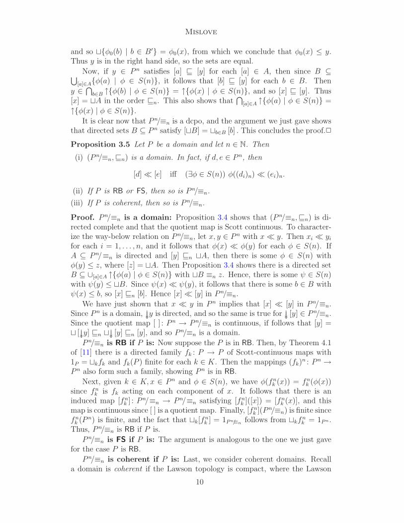
Proposition 3.5 Let P be a domain and let n ∈ N. Then

(i) (P n/≡n,⊑n) is a domain. In fact, if d, e ∈ P n, then

[d] ≪ [e] iff (∃φ ∈ S(n)) φ((di)n) ≪ (ei)n.

(ii) If P is RB or FS, then so is P n/≡n.

(iii) If P is coherent, then so is P n/≡n.

Proof. P n/≡n is a domain: Proposition 3.4 shows that (P n/≡n,⊑n) is di-rected complete and that the quotient map is Scott continuous. To character-ize the way-below relation on P n/≡n, let x, y ∈ P n with x≪ y. Then xi ≪ yi

for each i = 1, . . . , n, and it follows that φ(x) ≪ φ(y) for each φ ∈ S(n). IfA ⊆ P n/≡n is directed and [y] ⊑n ⊔A, then there is some φ ∈ S(n) withφ(y) ≤ z, where [z] = ⊔A. Then Proposition 3.4 shows there is a directed setB ⊆ ∪[a]∈A ↑{φ(a) | φ ∈ S(n)} with ⊔B ≡n z. Hence, there is some ψ ∈ S(n)with ψ(y) ≤ ⊔B. Since ψ(x) ≪ ψ(y), it follows that there is some b ∈ B withψ(x) ≤ b, so [x] ⊑n [b]. Hence [x] ≪ [y] in P n/≡n.

We have just shown that x ≪ y in P n implies that [x] ≪ [y] in P n/≡n.Since P n is a domain, ↓↓y is directed, and so the same is true for ↓↓ [y] ∈ P n/≡n.Since the quotient map [ ] : P n → P n/≡n is continuous, if follows that [y] =⊔ [↓↓y] ⊑n ⊔↓↓ [y] ⊑n [y], and so P n/≡n is a domain.

P n/≡n is RB if P is: Now suppose the P is in RB. Then, by Theorem 4.1of [11] there is a directed family fk : P → P of Scott-continuous maps with1P = ⊔kfk and fk(P ) finite for each k ∈ K. Then the mappings (fk)

n : P n →P n also form such a family, showing P n is in RB.

Next, given k ∈ K, x ∈ P n and φ ∈ S(n), we have φ(fnk (x)) = fn

k (φ(x))since fn

k is fk acting on each component of x. It follows that there is aninduced map [fn

k ] : P n/≡n → P n/≡n satisfying [fnk ]([x]) = [fn

k (x)], and thismap is continuous since [ ] is a quotient map. Finally, [fn

k ](P n/≡n) is finite sincefn

k (P n) is finite, and the fact that ⊔k[fnk ] = 1P n/≡n

follows from ⊔kfnk = 1P n.

Thus, P n/≡n is RB if P is.

P n/≡n is FS if P is: The argument is analogous to the one we just gavefor the case P is RB.

P n/≡n is coherent if P is: Last, we consider coherent domains. Recalla domain is coherent if the Lawson topology is compact, where the Lawson

10

Mislove

topology has the family of sets {U \ ↑F | F ⊆ P finite & U Scott open} for abasis. Now, if x ∈ P n, then {φ(x) | φ ∈ S(n)} is finite, and so if F ⊆ P n/≡n

is finite, then [↑F ]−1 = ∪[x]∈F ↑{φ(x) | φ ∈ S(n)} is finitely generated. Itfollows that [ ] : P n → P n/≡n is Lawson continuous, so if P is coherent, thenso are P n and P n/≡n. 2

Definition 3.6 Let P and Q be domains, and let f : P → Q be Scott con-tinuous. We let

(i) Bn(P ) = (P n/≡n,⊑n) denote the domain of n-bags over P . If n = 0,we identify P 0 with [〈〉], the equivalence class of the empty word overP . We also let Bn(f) : Bn(P ) → Bn(Q) be the induced map satisfyingBn(f)([d]P ) = [fn(d)]Q for all d ∈ P n, where [ ]P : P n → P n/≡n is thequotient map, and likewise for [ ]Q.

(ii) B(P ) =·

∪n Bn(P ) denote the disjoint sum 8 of the Bn(P ). We also let

B(f) =·

∪n Bn(f).

(iii) B⊥(P ) = ⊕nBn(P ) denote the separated sum 9 of the Bn(P ). We alsolet B⊥(f) be the extension of B(f) that sends ⊥ to ⊥.

Recall that if A is a category of dcpos, then A⊥ denotes the full subcat-egory of cpos in A, while A⊥,! denotes the subcategory of A⊥ of strict Scott-continuous maps, i.e., those that preserve least elements. We call A⊥,! thepointed subcategory determined by A.

Proposition 3.7

(i) Bn defines a continuous endofunctor on the categories DCPO, DOM,CDOM, RB and FS for each n ∈ N. Bn also defines a continuous endo-functor of the pointed subcategory determined by each of these categoriesof dcpos.

(ii) B defines a continuous endofunctor on DCPO and DOM.

(iii) B⊥ defines a continuous endofunctor on CPO!, the category of cpos andstrict Scott-continuous maps, and on CDOM⊥,!, RB⊥,! and FS⊥,!.

Proof. Ad (i): Proposition 3.5 shows that Bn(P ) is a domain if P is one. Iff : P → Q is Scott continuous, then so is fn : P n → Qn, and it is routine toshow that the mapping [d]P 7→ [fn(d)]Q, d ∈ P n is well-defined and continuous.Thus Bn is an endofunctor on CDOM, and it is defined as a compositionof constructors that define continuous endofunctors on each of the indicatedcategories, so it is continuous. Clearly [(⊥, . . . ,⊥)] is the least element ofBn(P ) if ⊥ is the least element of P , from which the claim about pointedsubcategories follows.

Ad (ii): For B, we must add the countable separated sum constructor,which it is easy to show leaves DCPO and DOM invariant.

8 The disjoint sum of dcpos is their disjoint union.9 The separated sum of (d)cpos is their disjoint union with a (new) bottom element added.

11

Mislove

Ad (iii): It is obvious that B⊥ leaves CPO invariant. A proof that each ofthe other pointed categories is closed under coalesced sums can be found in[1]. 2

3.1 Commutative domain monoids

By a domain monoid we mean a domain S equipped with a monoid operation· : S × S → S which is Scott continuous. For example, it is well known that

the family of finite words over P , P ∗ =def (·

∪P n, ·) where · is concatenation,is the free monoid over P , and hence the free domain monoid over P , if P isa domain. Of course, our interest is in commutative domain monoids – oneswhere the monoid operation is commutative.

Notation 3.8 We let CDM denote that category of commutative domainmonoids and Scott continuous monoid homomorphisms.

Theorem 3.9 Then B : DOM → CDM is left adjoint to the forgetful functor.

Proof. It is routine to show that B(P ) is a commutative monoid with respectto concatenation, with the empty word as the identity. Is (S, ∗) is any com-mutative monoid and f : P → S is Scott continuous, then there is a uniqueScott continuous monoid homomorphism f : P ∗ → S since (P ∗, ·) is the free

domain monoid over P . But since S is commutative, the mapping f |P n factorsthrough the family Bn(P ) for each n ≥ 0, and so there is a unique inducedmonoid homomorphism B(f) : B(P ) → S. 2

The interesting question is how to proceed in the case of B⊥(P ), the sep-arated sum of the family of Bn(P ). There are two “obvious” ways to extendthe monoid operation on B(P ) to include the new least element:

(+) Define ⊥ ·x = x, so that ⊥ acts like an additive 0, or

(×) Define ⊥ ·x =⊥, so that ⊥ acts like a multiplicative 0.

In the first case, we would identify ⊥ with the equivalence class of the emptyword, [〈 〉], and the effect is to make the empty word the least element ofB⊥(P ). We denote this monoid by B+(P ). As we will see, the order on B+(P )is too coarse to support this monoid structure, so it has to be refined. Butit plays a crucial role in recapturing Varacca’s indexed valuations using ourtechniques.

Definition 3.10 If P is a domain, we let B+(P ) = ⊕n>0Bn(P ) denote theseparated sum of the family {Bn(P ) | n > 0}, in the order given by

[(di)m] ⊑ [(ej)n] iff (∃ι : m → n) 10 di ≤ eι(i) for i ∈ m, (9)

with the semigroup operation of B(P ) extended so that ⊥ ·x = x for allx ∈ B+(P ).

10 We identify m with the set {0, . . . , m − 1}, and similarly for n.

12

Mislove

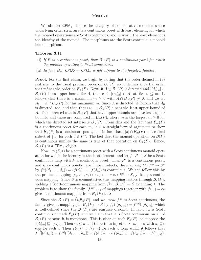
We also let CPM+ denote the category of commutative monoids whoseunderlying order structure is a continuous poset with least element, for whichthe monoid operations are Scott continuous, and in which the least element isthe identity of the monoid. The morphisms are the Scott-continuous monoidhomomorphisms.

Theorem 3.11

(i) If P is a continuous poset, then B+(P ) is a continuous poset for whichthe monoid operation is Scott continuous.

(ii) In fact, B+ : CPOS → CPM+ is left adjoint to the forgetful functor.

Proof. For the first claim, we begin by noting that the order defined in (9)restricts to the usual product order on Bn(P ), so it defines a partial orderthat refines the order on B⊥(P ). Next, if A ⊆ B+(P ) is directed and [(di)m] ∈B+(P ) is an upper bound for A, then each [(ai)n] ∈ A satisfies n ≤ m. Itfollows that there is a maximum m ≥ 0 with A ∩ Bm(P ) 6= ∅, and we letA0 = A ∩ Bm(P ) for this maximum m. Since A is directed, it follows that A0

is directed, too, and then that ⊔A0 ∈ Bm(P ) also is the least upper bound ofA. Thus directed sets in B+(P ) that have upper bounds are have least upperbounds, and these are computed in Bm(P ), where m is the largest m ≥ 0 forwhich the directed set intersects Bm(P ). From this and the fact that Bm(P )is a continuous poset for each m, it is a straightforward argument to showthat B+(P ) is a continuous poset, and in fact that ↓↓[d] ∩ Bm(P ) is a cofinalsubset of ↓↓[d] for each d ∈ Pm. The fact that the monoid operation on B(P )is continuous implies the same is true of that operation on B+(P ). Hence,B+(P ) is a CPM+-object.

Now, let (S, ∗) be a continuous poset with a Scott continuous monoid oper-ation for which the identity is the least element, and let f : P → S be a Scottcontinuous map with P a continuous poset. Then P n is a continuous poset,and since continuous posets have finite products, the mapping fn : P n → Sn

by fn((d1, . . . , dn)) = (f(d1), . . . , f(dn)) is continuous. We can follow this bythe product mapping (s1, . . . , sn) 7→ s1 ∗ · · · ∗ sn : Sn → S, yielding a contin-uous mapping. Since S is commutative, this mapping factors through Bn(P ),yielding a Scott-continuous mapping from f [n] : Bn(P ) → S extending f . Theproblem is to show the family {f [n]}n≥1 of mappings together with f(⊥) = ǫSgives a continuous mapping from B+(P ) to S.

Since the B+(P ) =·

∪nBn(P ), and we know f [n] is Scott continuous, thefamily gives a mapping f+ : B+(P ) → S by f+([(di)m]) = f [m]([(di)m]) whichis well-defined since the Bn(P )s are pairwise disjoint. In fact, f+ is Scottcontinuous on each Bn(P ), and we claim that it is Scott continuous on all ofB+(P ) because it is monotone. This is clear on each Bn(P ), so suppose the[(di)m] ⊑ [(ej)n]. Then m ≤ n and there is an injection ι : m → n with di ⊑P

eι(i) for each i. Then f(di) ⊑S f(eι(i)) for each i, from which it follows thatf+([(di)m]) = f [m]([(d1, . . . , dm]) = f(d1) ∗ · · · ∗ f(dm) ⊑S f(eι(1)) ∗ · · · f(eι(m)).

13

Mislove

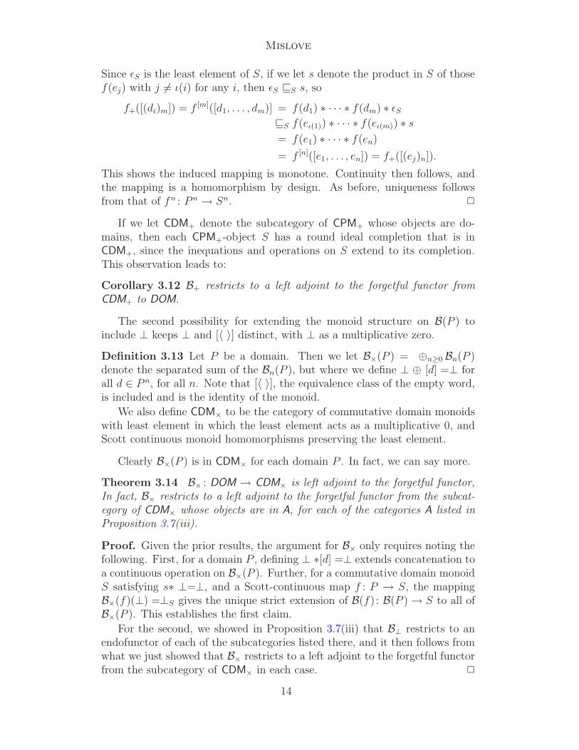
Since ǫS is the least element of S, if we let s denote the product in S of thosef(ej) with j 6= ι(i) for any i, then ǫS ⊑S s, so

f+([(di)m]) = f [m]([d1, . . . , dm)] = f(d1) ∗ · · · ∗ f(dm) ∗ ǫS⊑S f(eι(1)) ∗ · · · ∗ f(eι(m)) ∗ s

= f(e1) ∗ · · · ∗ f(en)

= f [n]([e1, . . . , en]) = f+([(ej)n]).

This shows the induced mapping is monotone. Continuity then follows, andthe mapping is a homomorphism by design. As before, uniqueness followsfrom that of fn : P n → Sn. 2

If we let CDM+ denote the subcategory of CPM+ whose objects are do-mains, then each CPM+-object S has a round ideal completion that is inCDM+, since the inequations and operations on S extend to its completion.This observation leads to:

Corollary 3.12 B+ restricts to a left adjoint to the forgetful functor fromCDM+ to DOM.

The second possibility for extending the monoid structure on B(P ) toinclude ⊥ keeps ⊥ and [〈 〉] distinct, with ⊥ as a multiplicative zero.

Definition 3.13 Let P be a domain. Then we let B×(P ) = ⊕n≥0 Bn(P )denote the separated sum of the Bn(P ), but where we define ⊥ ⊕ [d] =⊥ forall d ∈ P n, for all n. Note that [〈 〉], the equivalence class of the empty word,is included and is the identity of the monoid.

We also define CDM× to be the category of commutative domain monoidswith least element in which the least element acts as a multiplicative 0, andScott continuous monoid homomorphisms preserving the least element.

Clearly B×(P ) is in CDM× for each domain P . In fact, we can say more.

Theorem 3.14 B× : DOM → CDM× is left adjoint to the forgetful functor,In fact, B× restricts to a left adjoint to the forgetful functor from the subcat-egory of CDM× whose objects are in A, for each of the categories A listed inProposition 3.7(iii).

Proof. Given the prior results, the argument for B× only requires noting thefollowing. First, for a domain P , defining ⊥ ∗[d] =⊥ extends concatenation toa continuous operation on B×(P ). Further, for a commutative domain monoidS satisfying s∗ ⊥=⊥, and a Scott-continuous map f : P → S, the mappingB×(f)(⊥) =⊥S gives the unique strict extension of B(f) : B(P ) → S to all ofB×(P ). This establishes the first claim.

For the second, we showed in Proposition 3.7(iii) that B⊥ restricts to anendofunctor of each of the subcategories listed there, and it then follows fromwhat we just showed that B× restricts to a left adjoint to the forgetful functorfrom the subcategory of CDM× in each case. 2

14

Mislove

Example 3.15 We have shown that several Cartesian closed categories ofdomains are closed under the action of the functor B and its relatives. Hereis an example that demonstrates that the Cartesian closed category of Scottdomains does not enjoy this property. Let P = {⊥, a, b,⊤} be the four-element lattice with a and b incomparable, then P 2/≡2 is not in BCD: the pair[a,⊥], [b,⊥] has [a, b] and [⊤,⊥] as minimal upper bounds. 11

4 Reconstructing IVP (P )

We next use our results on bag domains to reconstruct Varacca’s Plotkin in-dexed valuations. We begin by considering how to introduce the non-negativereals into the picture. In fact, what we really want are commutative domainmonoids on which the non-negative reals act, so they should be modules overthe non-negative reals.

4.1 R+-spaces

The set R+ of positive reals is a continuous poset in the usual order. We saya continuous poset P is an R+-continuous poset if there is a Scott continuousmapping · : R+ × P → P satisfying mixed associativity: r · (s · p) = (rs) · p,for p ∈ P and r, s ∈ R+, and identity: 1 · p = p for all p ∈ P . We let CPOSR+

denote the category of R+-continuous posets and Scott continuous mappingsthat preserve the action: f(r · p) = r · f(p) for each r ∈ R+ and p ∈ P . Forany continuous poset P , its easy to create a continuous poset that contains Pand on which R+ acts:

Proposition 4.1 We define the functor BR+ : CPOS → CPOSR+ by BR+(P ) =R+ × P and for f : P → Q, BR+(f)(r, p) = (r, f(p)). Then BR+ is left adjointto the forgetful functor.

Moreover, if we let CPM denote the category of continuous posets whichare commutative monoids and whose morphisms are Scott-continuous monoidmaps, and if CPMR+ denotes the subcategory of CPM whose objects also admitR+ actions and whose morphisms respect that action, then BR+ restricts to aleft adjoint to the forgetful functor from CPMR+ to CPM.

Proof. The only interesting point is that the unit is the mapping p 7→(1, p) : P → R+ × P , which is guaranteed by the identity axiom. 2

4.2 Varacca’s indexed valuations

We now investigate two possibilities for how the identity of a commutativedomain monoid and the least element of the domain relate to one another: inone they are identified with one another, and in the other, they are distinct

11 Thanks to one of the anonymous referees for this example.

15

Mislove

elements; in the latter case we also treat the least element as a multiplica-tive zero. The first case allows us to recapture Varacca’s Plotkin indexedvaluations, as we now show.

Definition 4.2 Let P be a continuous poset. We define

BR

+(P ) = B+(R+ × P ) = ⊕n>0Bn(R+ × P )

to be the separated sum of the family {Bn(R+×P ) | n > 0}, and we define themonoid operation on BR

+(P ) to be the semigroup operation of B+(P ) extendedso that the new least element, ⊥, is the identity as well as the least element.We define an action of R≥0 on BR

+(P ) by

r · [(ri, di)m] = [(rri, di)m] and 0 · [(ri, di)m] = 0· ⊥ = r· ⊥ = ⊥,

for [(ri, di)m] ∈ BR

+(P ) and r ∈ R+. Then BR

+(P ) is a commutative monoidwhose underlying order structure is a continuous poset, on which R≥0 actsScott continuously.

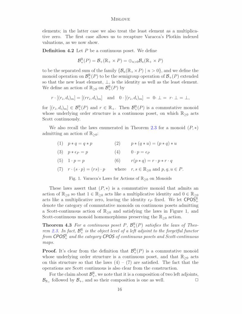
We also recall the laws enumerated in Theorem 2.3 for a monoid (P, ∗)admitting an action of R≥0:

(1) p ∗ q = q ∗ p (2) p ∗ (q ∗ u) = (p ∗ q) ∗ u

(3) p ∗ ǫP = p (4) 0 · p = ǫP

(5) 1 · p = p (6) r(p ∗ q) = r · p ∗ r · q

(7) r · (s · p) = (rs) · p where r, s ∈ R≥0 and p, q, u ∈ P .

Fig. 1. Varacca’s Laws for Actions of R≥0 on Monoids

These laws assert that (P, ∗) is a commutative monoid that admits anaction of R≥0 so that 1 ∈ R≥0 acts like a multiplicative identity and 0 ∈ R≥0

acts like a multiplicative zero, leaving the identity ǫP fixed. We let CPOSR

+

denote the category of commutative monoids on continuous posets admittinga Scott-continuous action of R≥0 and satisfying the laws in Figure 1, andScott-continuous monoid homomorphisms preserving the R≥0 action.

Theorem 4.3 For a continuous poset P , BR

+(P ) satisfies the laws of Theo-rem 2.3. In fact, BR

+ is the object level of a left adjoint to the forgetful functorfrom CPOSR

+ and the category CPOS of continuous posets and Scott-continuousmaps.

Proof. It’s clear from the definition that BR

+(P ) is a commutative monoidwhose underlying order structure is a continuous poset, and that R≥0 actson this structure so that the laws (4) – (7) are satisfied. The fact that theoperations are Scott continuous is also clear from the construction.

For the claim about BR

+, we note that it is a composition of two left adjoints,BR+ followed by B+, and so their composition is one as well. 2

16

Mislove

Remark 4.4 Recall that a continuous poset P can be completed into a do-main by taking its round-ideal completion, Id(P ). The resulting structurehas the same way-below relation as the underlying continuous poset, and infact it also has the same Scott topology. An equivalent way of realizing thisconstruction is to take the sobrification of P in its Scott topology.

Corollary 4.5 For a domain P , IVP (P ) ≃ Id(BR

+(P )).

Proof. One proof follows by noting that the mapping 〈ri, pi〉n 7→ [(ri, pi)n]and 0 7→⊥ defines a bijection of the indexed valuations over P onto BR

+(P )that takes ≪ in IVP (P ) to ≪ on BR

+(P ). Since they have isomorphic bases,the domains IVP (P ) and Id(BR

+(P )) are also isomorphic.

A perhaps more elegant proof follows by noting that BR

+(P ) satisfies thesame laws as IVP (P ), and both are initial objects over P according to Theo-rems 2.3 and 4.3. 2

Corollary 4.6 IdBR

+ generates a monad on DOM, and each of the powerdomain monads PX lifts to a monad on IdBR

+-algebras.

Proof. For each of the power domain monads, PX , Varacca showed that thereis a distributive law of IVP over PX in [23], and this implies that PX lifts toa monad on the class of IdBR

+-algebras by Beck’s Theorem 1.1 [2] and byTheorem 4.5. In fact, we can easily recover the distributive law that Varaccaobtains in [24] as follows: For a domain P , a power domain monad PX andan element [(ri, Xi)n] ∈ BR

+PX(P ), the distributive law on the basis elementsin BR

+(P ) is

d : BR

+PX.

−→ PXBR

+ by dP ([(ri, Xi)n]) = 〈[(ri, xi)n] | xi ∈ Xi ∈ PX(P )〉,

where 〈− 〉 denotes the element of PXBR

+(P ) generated by ∪i≤n{[(ri, xi)n] |xi ∈ Xi ∈ PX(P )}. The result follows from Beck’s Theorem 1.1 [2]. 2

Remark 4.7 For all its attractiveness, the shortcoming of Varacca’s indexedvaluations approach is that it is not clear whether it leaves any ccc’s of do-mains invariant. There is some relevant literature here: Poigne [21] showsthat there are no left adjoints for commutative semigroups or commutativeidempotent monoids over domains, if one includes a least element in the dis-cussion. Gordon Plotkin has also commented in a personal communicationthat he once showed that the free commutative semigroup with least elementtakes one out of the largest ccc of ω-algebraic domains, but that the argumentwould fail in the continuous case. Finally, Heckmann [6] has shown that thereis a lower bag domain construction that does not leave any ccc of algebraicdomains invariant, but again his arguments rely on the characterization ofbifinite domains, and it is not clear if they can be generalized to the settingwhere one is dealing with continuous objects.

So, this issue remains unresolved for Varacca’s construction. In the nextsection, we present an alternative that sacrifices one of the laws of Theorem 2.3,but gains the property of staying within ccc’s of domains.

17

Mislove

4.3 Real domain monoids

We now turn our attention to the action of R+ on other possible commutativedomain monoids with least element, namely ones in which the monoid identityis not the least element. Here is a weakening of Varacca’s laws to address thissituation.

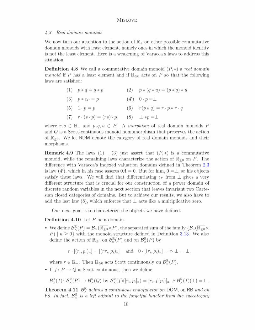
Definition 4.8 We call a commutative domain monoid (P, ∗) a real domainmonoid if P has a least element and if R≥0 acts on P so that the followinglaws are satisfied:

(1) p ∗ q = q ∗ p (2) p ∗ (q ∗ u) = (p ∗ q) ∗ u

(3) p ∗ ǫP = p (4′) 0 · p =⊥

(5) 1 · p = p (6) r(p ∗ q) = r · p ∗ r · q

(7) r · (s · p) = (rs) · p (8) ⊥ ∗p =⊥

where r, s ∈ R+ and p, q, u ∈ P . A morphism of real domain monoids Pand Q is a Scott-continuous monoid homomorphism that preserves the actionof R≥0. We let RDM denote the category of real domain monoids and theirmorphisms.

Remark 4.9 The laws (1) – (3) just assert that (P, ∗) is a commutativemonoid, while the remaining laws characterize the action of R≥0 on P . Thedifference with Varacca’s indexed valuation domains defined in Theorem 2.3is law (4′), which in his case asserts 0A = 0. But for him, 0 =⊥, so his objectssatisfy these laws. We will find that differentiating ǫP from ⊥ gives a verydifferent structure that is crucial for our construction of a power domain ofdiscrete random variables in the next section that leaves invariant two Carte-sian closed categories of domains. But to achieve our results, we also have toadd the last law (8), which enforces that ⊥ acts like a multiplicative zero.

Our next goal is to characterize the objects we have defined.

Definition 4.10 Let P be a domain.

• We define BR

×(P ) = B×(R≥0×P ), the separated sum of the family {Bn(R≥0×P ) | n ≥ 0} with the monoid structure defined in Definition 3.13. We alsodefine the action of R≥0 on BR

n (P ) and on BR

×(P ) by

r · [(ri, pi)n] = [(rri, pi)n] and 0 · [(ri, pi)n] = r· ⊥ = ⊥,

where r ∈ R+. Then R≥0 acts Scott continuously on BR

×(P ).

• If f : P → Q is Scott continuous, then we define

BR

×(f) : BR

×(P ) → BR

×(Q) by BR

×(f)([ri, pi]n) = [ri, f(pi)]n ∧ BR

×(f)(⊥) =⊥ .

Theorem 4.11 BR

× defines a continuous endofunctor on DOM, on RB and onFS. In fact, BR

× is a left adjoint to the forgetful functor from the subcategory

18

Mislove

of real domain monoids of each of these categories.

Proof. The arguments are similar to those given in the proof of Theorem 4.3,with the distinguishing feature of this construction that the least element isnot the monoid identity, but instead acts like a multiplicative zero relative tothe monoid operation, and that 0 · x =⊥ for all x ∈ BR

×(P ). 2

Remark 4.12

(i) For a poset P , the difference between BR

+(P ) and BR

×(P ) is that the leastelement of BR

+(P ) acts like a multiplicative identity, while in BR

×(P ), itacts as a multiplicative zero.

(ii) We have seen that BR

+(P ) allows us to recapture Varacca’s Plotkin in-dexed valuations over P . In so doing, we must form an ideal completion,because the order on BR

+(P ) is incomplete, even if P is a dcpo. Thisis because elements of the form [(ri, di)m] and [(sj , ej)n] can compare inBR

+(P ) even if m 6= n. In fact, it is easy to show that BR

+(P ) is directed,and so there is a largest element in its round ideal completion. It wouldbe interesting to study what role this element plays in the structure ofthe object.

(iii) On the other hand, BR

×(P ) is a domain if P is one, so no completionis necessary. Its least element is distinct from the monoid identity, andthe order prevents elements of the form [(ri, di)m] and [(sj, ej)n] fromcomparing unless m = n.

5 Discrete random variables over domains

We now show how to construct two power domains of discrete random variablesover a domain, one for each of our constructions, BR

+ and BR

×. We also showthat the second of these leaves some Cartesian closed categories of domainsinvariant.

To begin, recall that a random variable is a function f : (X,µ) → (Y,Σ)where (X,µ) is a probability space, (Y,Σ) is a measure space, and f is ameasurable function, which means f−1(A) is measurable in X for every A ∈ Σ,the specified σ-algebra of subsets of Y . Most often random variables take theirvalues in R, equipped with the usual Borel σ-algebra. For us, X will be acountable, discrete space, and Y will be a domain, where Σ will be the Borelσ-algebra generated by the Scott-open subsets.

Given a random variable f : X → Y , the usual approach is to “push theprobability measure µ forward” onto Y by defining fµ (A) = µ(f−1(A)) foreach measurable subset A of Y . But this defeats one of the attractions ofrandom variables: namely, that there may be several points x ∈ X which ftakes to the same value y ∈ Y . This is ‘attractive’ because it means that therandom variable f makes distinctions that the probability measure fµ doesnot, and we would like to exploit this fact. Varacca makes exactly this point

19

Mislove

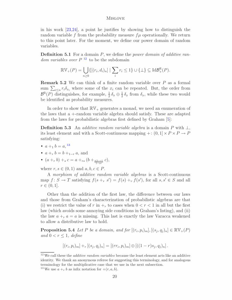
in his work [23,24], a point he justifies by showing how to distinguish therandom variable f from the probability measure fµ operationally. We returnto this point later. For the moment, we define our power domain of randomvariables.

Definition 5.1 For a domain P , we define the power domain of additive ran-dom variables over P 12 to be the subdomain

RV+(P ) =⋃

n≥0

{[(ri, di)n] |∑

i

ri ≤ 1} ∪ {⊥} ⊆ IdBR

+(P ).

Remark 5.2 We can think of a finite random variable over P as a formalsum

∑i≤n riδxi

where some of the xi can be repeated. But, the order from

BR(P ) distinguishes, for example, 12δx ⊕ 1

2δx from δx, while these two would

be identified as probability measures.

In order to show that RV+ generates a monad, we need an enumeration ofthe laws that a +-random variable algebra should satisfy. These are adaptedfrom the laws for probabilistic algebras first defined by Graham [5]:

Definition 5.3 An additive random variable algebra is a domain P with ⊥,its least element and with a Scott-continuous mapping +: (0, 1]×P ×P → Psatisfying:

• a+1 b = a, 13

• a+r b = b+1−r a, and

• (a+r b) +s c = a+rs (b+ s(1−r)1−sr

c),

where r, s ∈ (0, 1) and a, b, c ∈ P .

A morphism of additive random variable algebras is a Scott-continuousmap f : S → T satisfying f(s +r s

′) = f(s) +r f(s′), for all s, s′ ∈ S and allr ∈ (0, 1].

Other than the addition of the first law, the difference between our lawsand those from Graham’s characterization of probabilistic algebras are that(i) we restrict the value of r in +r to cases when 0 < r < 1 in all but the firstlaw (which avoids some annoying side conditions in Graham’s listing), and (ii)the law a +r a = a is missing. This last is exactly the law Varacca weakenedto allow a distributive law to hold.

Proposition 5.4 Let P be a domain, and for [(ri, pi)m], [(sj , qj)n] ∈ RV+(P )and 0 < r ≤ 1, define

[(ri, pi)m] +r [(sj , qj)n] = [(rri, pi)m]⊕ [((1 − r)sj, qj)n] .

12 We call these the additive random variables because the least element acts like an additiveidentity. We thank an anonymous referee for suggesting this terminology, and for analogousterminology for the multiplicative case that we use in the next subsection.13 We use a +r b as infix notation for +(r, a, b).

20

Mislove

Then:

(i) RV+(P ) is an additive random variable algebra, and

(ii) [(r, p)] = [(1, p)]+r ⊥ for all p ∈ P and all r ∈ (0, 1), and

[(r1, p1), . . . , (rm, pm)] = [(1, p1)] +r1 [(r2

(1 − r1), p2), . . . , (

rm

(1 − r1), pm)]

for all [(r1, p1), . . . , (rm, pm)] ∈ RV+(P ).

Proof. Given a domain P , we can define +: (0, 1] × BR(P )2 → BR(P ) by

+(r, [(ri, pi)m], [(sj, qj)n] = [(rri, pi)m]⊕ [((1 − r)sj, qj)n] .

Because R+ acts continuously on BR

+(P ) and because ⊕ is continuous, + is acontinuous operation. RV+(P ) is the subfamily of IdBR

+(P ) whose real compo-nents are bounded by 1, and this family is clearly invariant under the action ofR+, so this defines a continuous mapping +: (0, 1]×RV+(P )2 → RV+(P ). Us-ing the abbreviation that [(ri, pi)m] +r [(sj , qj)n] = [(rri, pi)m]⊕ [((1 − r)sj, qj)n],it also is routine to verify that the laws of Definition 5.3 are satisfied.

The results in (ii) are simple calculations. 2

We now characterize the initial additive random variable algebra over adomain.

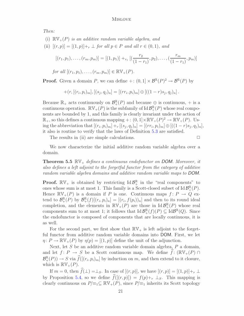
Theorem 5.5 RV+ defines a continuous endofunctor on DOM. Moreover, italso defines a left adjoint to the forgetful functor from the category of additiverandom variable algebra domains and additive random variable maps to DOM.

Proof. RV+ is obtained by restricting IdBR

+ in the “real components” toones whose sum is at most 1. This family is a Scott-closed subset of IdBR

+(P ).Hence RV+(P ) is a domain if P is one. Continuous maps f : P → Q ex-tend to BR

+(P ) by BR

+(f)[(ri, pi)n] = [(ri, f(pi))n] and then to its round idealcompletion, and the elements in RV+(P ) are those in IdBR

+(P ) whose realcomponents sum to at most 1; it follows that IdBR

+(f)(P ) ⊆ IdBR(Q). Sincethe endofunctor is composed of components that are locally continuous, it isas well.

For the second part, we first show that RV+ is left adjoint to the forget-ful functor from additive random variable domains into DOM. First, we letη : P → RV+(P ) by η(p) = [(1, p)] define the unit of the adjunction.

Next, let S be an additive random variable domain algebra, P a domain,and let f : P → S be a Scott continuous map. We define f : (RV+(P ) ∩

BR

+(P )) → S via f([(ri, pi)m] by induction on m, and then extend to it closure,which is RV+(P ).

If m = 0, then f(⊥) =⊥S. In case of [(r, p)], we have [(r, p)] = [(1, p)]+r ⊥

by Proposition 5.4, so we define f([(r, p)]) = f(p)+r ⊥S. This mapping isclearly continuous on P/≡1⊆ RV+(P ), since P/≡1 inherits its Scott topology

21

Mislove

from that of RV+(P ). This is also the unique such function on P/≡1 satisfying

f ◦ η = f .

Continuing the definition of f by induction, assume that we have definedf on ∪k≤n(P

k/≡k) uniquely so that it is continuous and satisfies f ◦ η = f .Let [(r1, p1), . . . , (rm+1, pm+1)] ∈ Pm+1/≡m+1, and then define

f([(r1, p1), . . . , (rm+1, pm+1)]) = f(p1) +r1 f([(r2

1 − r1, p2), . . . , (

rm+1

1 − r1, pm+1)].

This is well-defined by Proposition 5.4(ii), and it is the composition of con-

tinuous functions, so it is continuous. It also satisfies f ◦ η = f because it’srestriction to P/≡1 does by definition. Finally, Proposition 5.4(ii) again showsit is the unique such function.

This shows that RV+ is left adjoint to the forgetful functor from randomvariable algebras into DOM, so it generates a monad on DOM. 2

Corollary 5.6 Each of the power domain monads PX lifts to a monad onRV+-algebras.

Proof. The distributive law given in the proof of Corollary 4.6 clearly restrictsto one for RV+. 2

This corollary means we can solve domain equations such as P ≃ PX ◦RV+(P ) for each of the power domain monads PX . The resulting domain Pwill be a PX -algebra and simultaneously a RV+-algebra.

5.1 Discrete random variables for Cartesian closed categories

We now use our functor BR

× to define a second construction of random variablesover domains. This one has the advantage of leaving some Cartesian closedcategories of domains invariant. Since the results parallel those of the lastsubsection, with BR

× replacing BR

+, we confine the proofs to pointing out thosearguments that vary from the ones in the last subsection.

Definition 5.7 For a domain P , we define the power domain of multiplicativerandom variables over P to be the subdomain

RV×(P ) =⋃

n≥0

{[(ri, di)n] |∑

i

ri ≤ 1} ∪ {⊥} ⊆ BR

×(P ).

The laws that a multiplicative random variable algebra should satisfy varyonly slightly from those for additive random variable algebras from the lastsubsection:

Definition 5.8 A multiplicative random variable algebra is a domain P with0, its identity element and with a Scott-continuous mapping +: (0, 1] × P ×P → P satisfying:

• ⊥ +r a =⊥ for all 0 < r ≤ 1,

22

Mislove

• a+1 b = a,

• a+r b = b+1−r a, and

• (a+r b) +s c = a+rs (b+ s(1−r)1−sr

c),

where r, s ∈ (0, 1) and a, b, c ∈ P .

A morphism of multiplicative random variable algebras is a Scott-continuousmap f : S → T satisfying f(0S) = 0T , f(⊥S) =⊥T and f(s +r s

′) = f(s) +r

f(s′), for all s, s′ ∈ S and all r ∈ (0, 1].

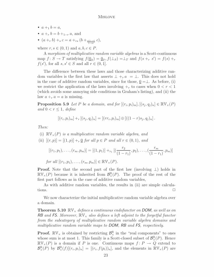
The difference between these laws and those characterizing additive ran-dom variables is the first law that asserts ⊥ +r a = ⊥. This does not holdin the case of additive random variables, since for those, 0 =⊥. As before, (i)we restrict the application of the laws involving +r to cases when 0 < r < 1(which avoids some annoying side conditions in Graham’s listing), and (ii) thelaw a+r a = a is missing.

Proposition 5.9 Let P be a domain, and for [(ri, pi)m], [(sj , qj)n] ∈ RV×(P )and 0 < r ≤ 1, define

[(ri, pi)m] +r [(sj , qj)n] = [(rri, pi)m]⊕ [((1 − r)sj, qj)n] .

Then:

(i) RV×(P ) is a multiplicative random variable algebra, and

(ii) [(r, p)] = [(1, p)] +r 0 for all p ∈ P and all r ∈ (0, 1), and

[(r1, p1), . . . , (rm, pm)] = [(1, p1)] +r1 [(r2

(1 − r1), p2), . . . , (

rm

(1 − r1), pm)]

for all [(r1, p1), . . . , (rm, pm)] ∈ RV×(P ).

Proof. Note that the second part of the first law (involving ⊥) holds inRV×(P ) because it is inherited from BR

×(P ). The proof of the rest of thefirst part follows as in the case of additive random variables,

As with additive random variables, the results in (ii) are simple calcula-tions. 2

We now characterize the initial multiplicative random variable algebra overa domain.

Theorem 5.10 RV× defines a continuous endofunctor on DOM, as well as onRB and FS. Moreover, RV× also defines a left adjoint to the forgetful functorfrom the subcategory of multiplicative random variable algebra domains andmultiplicative random variable maps to DOM, RB and FS, respectively.

Proof. RV× is obtained by restricting BR

× in the “real components” to oneswhose sum is at most 1. This family is a Scott-closed subset of BR

×(P ). HenceRV×(P ) is a domain if P is one. Continuous maps f : P → Q extend toBR

×(P ) by BR

×(f)[(ri, pi)n] = [(ri, f(pi))n], and the elements in RV×(P ) are

23

Mislove

those in BR

×(P ) whose real components sum to at most 1; it follows thatBR

×(f)(P ) ⊆ BR(Q). Since the endofunctor is composed of components thatare locally continuous, it is as well.

For the second part, we first show that RV× is left adjoint to the forgetfulfunctor from multiplicative random variable domains into DOM. First, we letη : P → RV×(P ) by η(p) = [(1, p)] define the unit of the adjunction.

Next, let S be a multiplicative random variable domain algebra, P a do-main, and let f : P → S be a Scott continuous map. We define f : (RV×(P )∩

BR

×(P )) → S via f([(ri, pi)m] by induction on m, just as in the case of RV+(P ),and the argument is virtually the same.

This shows that RV× is left adjoint to the forgetful functor from randomvariable algebras into DOM, so it generates a monad on DOM. We have alreadyshown that RV×(P ) is in RB or FS if P is, so RV× has restrictions to thesesubcategories that also define monads. 2

Corollary 5.11 Each of the power domain monads PX lifts to a monad onRV×-algebras. 2

As in the case of RV×, we can solve domain equations such as P ≃ PX ◦RV×(P ) for each of the power domain monads PX . The resulting domain Pwill be a PX -algebra and simultaneously a RV×-algebra. What’s true now,though, is that these domain equations can be solved within Cartesian closedcategories of domains.

5.2 Random variables and probability measures

One might also ask about the relationship between our construction and thetraditional probabilistic power domain over a domain. The following providesthe answer.

Theorem 5.12 If P is a domain, then there is an epimorphism F lat : RV+(P )→ V(P ), the domain of subprobability measures over P . Similarly, there is anepimorphism F lat : RV×(P ) → V(P ).

Proof. In both cases, the mapping is F lat([ri, di]n) =∑

i≤n riδdi, where in

V(P ), summands with the same support are identified. This is easily seen todefine a Scott-continuous map in both cases. It is an epimorphism of domainsbecause the simple valuations are dense [10], and clearly they are the range ofF lat. 2

6 Summary and Future Work

We have presented two power domains for discrete random variables, andshown that each of them defines a monad on domains that enjoy distribu-tive laws with respect to each of the power domain monads. Moreover, our

24

Mislove

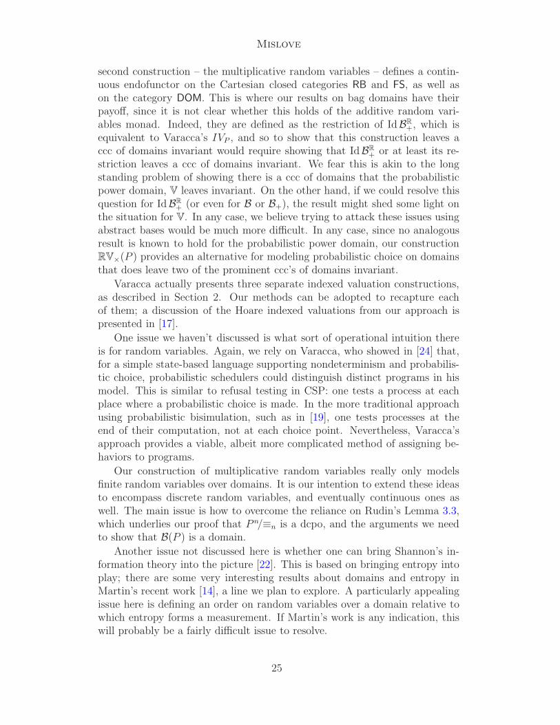
second construction – the multiplicative random variables – defines a contin-uous endofunctor on the Cartesian closed categories RB and FS, as well ason the category DOM. This is where our results on bag domains have theirpayoff, since it is not clear whether this holds of the additive random vari-ables monad. Indeed, they are defined as the restriction of IdBR

+, which isequivalent to Varacca’s IVP , and so to show that this construction leaves accc of domains invariant would require showing that IdBR

+ or at least its re-striction leaves a ccc of domains invariant. We fear this is akin to the longstanding problem of showing there is a ccc of domains that the probabilisticpower domain, V leaves invariant. On the other hand, if we could resolve thisquestion for IdBR

+ (or even for B or B+), the result might shed some light onthe situation for V. In any case, we believe trying to attack these issues usingabstract bases would be much more difficult. In any case, since no analogousresult is known to hold for the probabilistic power domain, our constructionRV×(P ) provides an alternative for modeling probabilistic choice on domainsthat does leave two of the prominent ccc’s of domains invariant.

Varacca actually presents three separate indexed valuation constructions,as described in Section 2. Our methods can be adopted to recapture eachof them; a discussion of the Hoare indexed valuations from our approach ispresented in [17].

One issue we haven’t discussed is what sort of operational intuition thereis for random variables. Again, we rely on Varacca, who showed in [24] that,for a simple state-based language supporting nondeterminism and probabilis-tic choice, probabilistic schedulers could distinguish distinct programs in hismodel. This is similar to refusal testing in CSP: one tests a process at eachplace where a probabilistic choice is made. In the more traditional approachusing probabilistic bisimulation, such as in [19], one tests processes at theend of their computation, not at each choice point. Nevertheless, Varacca’sapproach provides a viable, albeit more complicated method of assigning be-haviors to programs.

Our construction of multiplicative random variables really only modelsfinite random variables over domains. It is our intention to extend these ideasto encompass discrete random variables, and eventually continuous ones aswell. The main issue is how to overcome the reliance on Rudin’s Lemma 3.3,which underlies our proof that P n/≡n is a dcpo, and the arguments we needto show that B(P ) is a domain.

Another issue not discussed here is whether one can bring Shannon’s in-formation theory into the picture [22]. This is based on bringing entropy intoplay; there are some very interesting results about domains and entropy inMartin’s recent work [14], a line we plan to explore. A particularly appealingissue here is defining an order on random variables over a domain relative towhich entropy forms a measurement. If Martin’s work is any indication, thiswill probably be a fairly difficult issue to resolve.

25

Mislove

Acknowledgment We wish to thank several people for their comments aboutthis work. The list includes Samson Abramsky, Gavin Lowe, Keye Martin,Dusko Pavlovic, Bill Roscoe and James Worrell. We also would like to thankanonymous referees both of this paper and of its predecessor [18] for manyvaluable suggestions.

References

[1] Abramsky, S. and A. Jung, “Domain Theory,” in: Handbook of Logic inComputer Science, S. Abramsky and D. M. Gabbay and T. S. E. Maibaum,editors, Clarendon Press, 1994, pp. 1—168.

[2] Beck, J., Distributive laws, in: Seminar on Triples and Categorical Homology

Theory, 1969, pp. 119–140.

[3] Gautam, N. D., The validity of equations of complex algebras, Archiv furMathematische Logik und Grundlagenforschung 3 (1957), pp. 117–124.

[4] Gierz, G., K. H. Hofmann, K. Keimel, J. Lawson, M. Mislove and D. Scott,“Continuous Lattices and Domains,” Cambridge University Press, 2003.

[5] Graham, S. K., Closure properties of a probabilistic domain construction, LectureNotes in Computer Science 298 (1985), pp. 213–233.

[6] Heckmann, Reinhold, Lower bag domains. Fundamenta Informaticae 24 (1995),pp. 259–281.

[7] Hennessy, M. and G. D. Plotkin, Full abstraction for a simple parallel

programming language, Lecture Notes in Computer Science 74 (1979), pp. 108–120.

[8] Johnstone, P. T., Partial products, bag domains and hyperlocal toposes, LMSLecture Notes Series 77 (1992), pp. 315–339.

[9] Johnstone, P. T., Variations on a bagdomain theme, Theoretical ComputerScience 136 (1994), pp. 3–20.

[10] Jones, C., “Probabilistic Nondeterminism,” PhD Dissertation, University ofEdinburgh, Scotland, 1989.

[11] Jung, A., “Cartesian Closed Categories of Domains,” CWI Tracts 66 (1989),Centrum voor Wiskunde en Informatica, Amsterdam.

[12] Jung, A. and R. Tix, The troublesome

probabilistic power domain, Electronic Notes in Theoretical Computer Science13 (1999), http://www.elsevier.com/locate/entcs/volume13.html

[13] Lowe, G., “Probabilities and Priorities in Timed CSP,” DPhil Thesis, OxfordUniversity, 1993.

[14] Martin, K. Entropy as a fixed point, Proceedings of ICALP 2004, LNCS 3142,2004.

26

Mislove

[15] Mislove, M. Algebraic posets, algebraic cpos and models of concurrency,

Proceedings of the Oxford Symposium on Topology, G. M. Reed, A. W. Roscoeand R. Wachter, editors, Oxford University Press, 75 – 111.

[16] Mislove, M. Nondeterminism and probabilistic choice: Obeying the laws, LectureNotes in Computer Science 1877 (2000), pp. 350–364.

[17] Mislove, M. Monoids over domains, Mathematical Structures for Computer

Science, to appear.

[18] Mislove, M., Discrete random variables over domains, Proceedings of ICALP2005, Lecture Notes in Computer Science 3580 (2005), pp. 1006–1017.

[19] Mislove, M., J. Ouaknine and J. B. Worrell, Axioms for probability and

nondeterminism, Proceedings of EXPRESS 2003, Electronic Notes in TheoreticalComputer Science 91(3), Elsevier.

[20] Plotkin, G. D., “Domains,” The Pisa Notes, 1983, available at URLhttp://homepages.inf.ed.ac.uk/gdp/publications/.

[21] Poigne, A., A remark on variations of power domains, Bulletin of the EATCS31 (1987), pp. 38–41.

[22] Shannon, C., A mathematical theory of information, Bell Systems TechnicalJournal 27 (1948), pp. 379–423 & 623–656.

[23] Varacca, D., The powerdomain of indexed valuations, Proceedings 17th IEEESymposium on Logic in Computer Science (LICS 2002), IEEE Press, 2002.

[24] Varacca, D., “Probability, Nondeterminism and Concurrency: Two Denotation-al Models for Probabilistic Computation,” PhD Dissertation, Aarhus University,Aarhus, Denmark, 2003.

[25] Vickers, S. Geometric theories and databases, LMS Lecture Notes Series 77(1992), pp. 288–314.

27