Discrete Morphology with Line Structuring Elements

C.L. Luengo Hendriks, L.J. van Vliet

Pattern Recognition GroupDepartment of Applied PhysicsDelft University of Technology

Lorentzweg 1, 2628 CJ Delft, The Netherlandscris@ph.tn.tudelft.nl

Keywords: interpolation, skewing, Bresenham line, periodic line, band-limited line, image processing

Abstract

Discrete morphological operations with line seg-ments are notoriously hard to implement. In this pa-per we study different possible implementations of theline structuring element, compare them, and exam-ine their rotation and translation invariance in thecontinuous-domain sense. That is, we are interestedin obtaining a morphological operator that is invari-ant to rotations and translations of the image beforesampling.

1 Introduction

Morphological operations use a structuring ele-ment (SE), which plays the role of a neighborhoodor convolution kernel in other image-processing oper-ations. Often, these SEs are composed of line seg-ments. For example, the square, hexagon and oc-tagon, which are increasingly accurate approxima-tions of the disk, can be decomposed into two, threeand four line segments respectively [11, 12]. Thus,it is possible to create an arbitrarily accurate approxi-mation of a disk by increasing the number of line seg-ments used. The advantage of using line segmentsinstead of N-dimensional structuring elements is areduction in the computational complexity. Further-more, it is possible to implement a dilation or erosionby a line segment under an arbitrary angle with only3 comparisons per pixel, irrespective of the length ofthe line segment, using a recursive algorithm [17, 13].

Adams [1] showed how to create an optimal dis-crete disk using dilations with line segments. Thesedisks are only approximations of the sampled Eu-clidean disk. The optimality is a trade-off betweenaccuracy and efficiency. For multi-scale closingswith these disks, however, absorption does not hold.Jones and Soille [5] improved on this by using peri-

odic lines, so that the absorption property is satisfied.Nonetheless, these SEs sacrifice accuracy to gain im-plementation efficiency. The actual implementationof the line structuring element is not very important,since the result is an approximation anyway.

Our reason to study the implementation of the lineSE is to improve on the result of morphological op-erations used to detect and measure linear features inimages. Examples are roads in airborne images [3, 6],grid patterns on stamped metal sheets [16], and struc-ture orientation estimation [14, 15]. We also use lineSEs in RIA Morphology [9, 10].

This paper is organized as follows. We start withan introduction to Bresenham lines, the basic discretelines. The most simple implementation of the di-lation uses a Bresenham line as SE. For efficiencypurposes, one might compute regional maxima overa Bresenham line across the image (using the recur-sive algorithm mentioned above). The drawback isthat this operation is not even translation-invariant inthe discrete sense (i.e. invariant over integer pixelshifts). Jones and Soille [5] introduced periodic lines,which are studied in Section 3. Using periodic lines,it is possible to construct recursive dilations that aretranslation-invariant in the discrete sense. After thatwe introduce operations obtained by interpolating theimage to obtain regional maxima over line segments(Sections 4 and 5), and a grey-value SE that imple-ments an approximately band-limited line segment(Section 6).

All of these approaches are compared in Sec-tion 7. We then test the two best methods for rotation-invariance and translation-invariance. Note that whenwe talk about translation-invariance, we actuallymean invariance to (sub-pixel) shifts of the samplinggrid; that is, translation-invariance in the continuous-domain sense (unless explicitly stated otherwise).

1

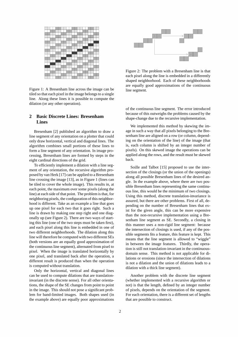
Figure 1: A Bresenham line across the image can betiled so that each pixel in the image belongs to a singleline. Along these lines it is possible to compute thedilation (or any other operation).

2 Basic Discrete Lines: BresenhamLines

Bresenham [2] published an algorithm to draw aline segment of any orientation on a plotter that couldonly draw horizontal, vertical and diagonal lines. Thealgorithm combines small portions of these lines toform a line segment of any orientation. In image pro-cessing, Bresenham lines are formed by steps in theeight cardinal directions of the grid.

To efficiently implement a dilation with a line seg-ment of any orientation, the recursive algorithm pro-posed by van Herk [17] can be applied to a Bresenhamline crossing the image [13], as in Figure 1 (lines canbe tiled to cover the whole image). This results in, ateach point, the maximum over some pixels (along theline) at each side of that point. The problem is that, forneighboring pixels, the configuration of this neighbor-hood is different. Take as an example a line that goesup one pixel for each two that it goes right. Such aline is drawn by making one step right and one diag-onally up (see Figure 2). There are two ways of start-ing this line (one of the two steps must be taken first),and each pixel along this line is embedded in one oftwo different neighborhoods. The dilation along thisline will therefore be computed with two different SEs(both versions are an equally good approximation ofthe continuous line segment), alternated from pixel topixel. When the image is translated horizontally byone pixel, and translated back after the operation, adifferent result is produced than when the operationis computed without translation.

Only the horizontal, vertical and diagonal linescan be used to compute dilations that are translation-invariant (in the discrete sense). For all other orienta-tions, the shape of the SE changes from point to pointin the image. This should not pose a significant prob-lem for band-limited images. Both shapes used (inthe example above) are equally poor approximations

Figure 2: The problem with a Bresenham line is thateach pixel along the line is embedded in a differentlyshaped neighborhood. Each of these neighborhoodsare equally good approximations of the continuousline segment.

of the continuous line segment. The error introducedbecause of this outweighs the problems caused by theshape-change due to the recursive implementation.

We implemented this method by skewing the im-age in such a way that all pixels belonging to the Bre-senham line are aligned on a row (or column, depend-ing on the orientation of the line) of the image (thatis, each column is shifted by an integer number ofpixels). On this skewed image the operations can beapplied along the rows, and the result must be skewedback.

Soille and Talbot [15] proposed to use the inter-section of the closings (or the union of the openings)along all possible Bresenham lines of the desired an-gle. In the example above, where there are two pos-sible Bresenham lines representing the same continu-ous line, this would be the minimum of two closings.Using this method, discrete translation-invariance isassured, but there are other problems. First of all, de-pending on the number of Bresenham lines that ex-ist for the given angle, this can be more expensivethan the non-recursive implementation using a Bre-senham line segment as SE. Secondly, a closing inthis manner uses a non-rigid line segment: becausethe intersection of closings is used, if any of the pos-sible segments fits a feature, this feature is kept. Thismeans that the line segment is allowed to “wiggle”in between the image features. Thirdly, the opera-tion is still not translation-invariant in the continuous-domain sense. This method is not applicable for di-lations or erosions (since the intersection of dilationsis not a dilation and the union of dilations leads to adilation with a thick line segment).

Another problem with the discrete line segment(whether implemented with a recursive algorithm ornot) is that the length, defined by an integer numberof pixels, depends on the orientation of the segment.For each orientation, there is a different set of lengthsthat are possible to construct.

2

Figure 3: The problem of the Bresenham line can besolved by using only a limited number of pixels onthe line. This way, each neighborhood is the same,although it is no longer connected. This is a periodicline.

⊕ =

Figure 4: By dilating a periodic line segment with asmall SE, it is possible to join up the SE. This lim-its the available lengths of the SE to multiples of theperiod.

3 Periodic Lines

Periodic lines were introduced by Jones andSoille [5] as a remedy to the (discrete) translation-invariance of the morphological operations along Bre-senham lines. A periodic line is composed of onlythose points of the continuous line that fall exactly ona grid point, see Figure 3. These lines are thus formedof disconnected pixels, except for lines of one of thethree cardinal orientations. When considering onlythese points, it is possible to use a recursive imple-mentation along the periodic lines that is translation-invariant in the discrete sense. However, because ofthe sparseness of the points along such a line, theyare not useful except in constructing more complexstructuring elements. For example, by dilating a pe-riodic line segment with a small connected segment,one creates a connected line segment, as in Figure 4.Thus, to implement a (discrete) translation-invariantdilation, one would compute a dilation with a periodicline segment, and on the result apply another dilationwith a small connected line segment (which does notneed to be implemented recursively because it is sosmall).

The drawbacks of this method are the small num-ber of orientations for which it is useful (there areonly few orientations that produce a short periodic-ity; for longer periodicities the line segment neededto connect the periodic line is longer as well), andthe limited number of lengths that can be created (thelength is a multiple of the periodicity, which dependson the orientation).

Because the result of this implementation is thesame as that obtained by a direct (non-recursive) im-

Skew

Figure 5: After skewing the image, horizontal linescorrespond to lines under a certain angle with respectto the image data. Some of the original image samplesfall exactly on these lines (·), but most samples used(◦) lie in between original grid points. The value atthese points is obtained by interpolation.

plementation using a Bresenham line segment as SE,we do not consider it separately in the comparison ofSection 7.

4 Interpolated Lines by Skewing of theImage

We mentioned above that operations along a Bre-senham line can be implemented by skewing the im-age, applying the operation along a column (or row),and skewing the image back. In this section we con-sider image skews with interpolation (that is, the rowsor columns of the image are not shifted by an integernumber of pixels, but by a real value). See Figure 5.

The interpolation method used is an important fac-tor in the correctness of the output. The better themethod is, the smaller the error will be. We used cubicconvolution [7] to implement the skews. This methodis a good compromise between accuracy, computa-tional cost and window size.1

The lines obtained in this way are interpolated,but have the same number of samples as the Bre-senham line of the same parameters. It is expectedthat these result in a somewhat better translation-invariance. The mayor drawback is that the resultneeds to be skewed back. As stated before, morpho-logical operations do not produce band-limited im-ages, and therefore the results are not sampled prop-erly. Interpolating the result of a morphological oper-ation is questionable at best.

The reason we need to interpolate in the resultingimage is that the result of the morphological operationis computed at the points along the continuous linelaid across the image, and not at the grid points ofthe output image. There are few columns (as manyas there are points in the periodic line representationfor the selected orientation) with zero or integer shift.

1Remember that the image is not infinite in size, and thereforeit is not possible to use the ideal interpolator. The window size isimportant because it determines the portion of the image affectedby the border.

3

Figure 6: At the expense of some extra computations,it is possible to directly compute each of the outputcolumns, so that the inverse skew is not required. Nothaving to interpolate in the result of a morphologicaloperation is the safest way.

For these columns, no interpolation of the output isrequired, and the result is at its best.

To improve the result on the other columns, itmight be interesting to sample the lines more denselybefore applying the morphological operation. Thismakes the inverse skew more accurate because thealiasing introduced by the operation will be less se-vere. In [8] we also used interpolation to increase theaccuracy of morphological operations.

5 True Interpolated Lines

The interpolated lines presented above are at theirbest on only a few columns (or rows) of the image.It is, of course, also possible to accomplish the sameaccuracy for all output pixels. In this case, for eachoutput pixel, samples along a line that goes exactlythrough it are computed by interpolation, as in Fig-ure 6. On these computed samples the operation isperformed.

To compute these lines somewhat efficiently, weresort again to the skew. By changing the offset of theimage for the skew, it is possible to select which groupof columns gets an integer shift. After performing theskew many times, different images are obtained. Eachof the columns of the input image is represented withinteger shift in one of these skewed images. After ap-plying the operation on the rows of these images, thecolumns with integer shifts can be extracted and usedto construct the output image. No interpolation needsto be performed in the output images of the opera-tion. The number of skews that need to be computedis equal to the periodicity of the periodic line acrossthe image.

Again, as for all discrete line segments mentionedup to now, the number of samples used in the com-putation of the morphological operation depends onboth the length of the segment and the orientation.Line segments along the grid are the densest, and di-agonal segments have the least number of samples.Thus, for some orientations it is more probable tomiss a local maximum (i.e. the maximum falls in

Figure 7: An approximately band-limited line seg-ment constructed with Equation (1).

between samples) than for others. This makes thecontinuous-domain translation-invariance better forhorizontal and vertical lines than for diagonal lines,and also has repercussions for the rotation-invariance.Ideally, one would like to sample each of these linesequally densely. To do so, it would be necessary toadd columns to the image when skewing. As men-tioned above, this also enables the creation of sub-pixel segment lengths, in a similar fashion to the in-terpolation used in [8] to increase the accuracy of theisotropic closing.

Alternatively, rotating the image instead of skew-ing it also alleviates this problem. However, whenrotating, only a limited set of samples falls exactlyon output samples, and in the worst case this happensonly for the sample in the origin of the rotation. Thismeans that a larger number of operations is requiredto compute the result of the operation at all outputpixels.

We have not corrected for the number of samplesalong the line segment in the comparison below.

6 Band-Limited Lines

A last option when implementing morphologywith discrete line segments is to use grey-value SEs,which allows to construct band-limited lines. Such asegment is rotation and translation invariant, and doesnot have a limited set of available lengths. The draw-back is that the line is thicker, but this should not be aproblem for band-limited images, since it should con-tain only thick lines as well.

A Gaussian function, as well as its integral, areband-limited in good approximation, and can be sam-pled at a rate of σ with a very small error [18]. Anapproximately band-limited line segment can be gen-erated using the error-function along the length of thesegment, and using the Gaussian function in the otherdimensions.

Let us define a two-dimensional image L(�,σ), to be

4

used as a structuring element, by

L(�,σ)(x,y) = A · exp

(−y2

2σ 2

)·

12

{1− erf

(�−2 |x|

2σ

)}, (1)

where � is the length of the line segment, x is the co-ordinate axis in the direction of the segment, and yis the coordinate axis perpendicular to it. Again, set-ting σ to 1 is enough to obtain a correctly sampledSE. Figure 7 shows an example of such a band-limitedline segment. Of course, generating line segments inhigher-dimensional images is trivial: y needs to besubstituted by a vector. Note that the grey-value of thesegment is 0, and the background has a value of −A.A is the scaling of the SE image, and should dependon the grey-value range in the image to be processed.

It is not directly clear, however, how to scale thisimage L(�,σ). It is obvious that the height A of the linesegment must be larger than the range of grey-valuesin the image. If it is not, the edge of the image used asSE will influence the morphological operation, whichis not desirable. But this height will also influence theshape of the segment. Even though the line segmentis approximately band-limited for any A, its slopes arenot invariant to this grey-value scaling. Since mor-phological operations can be written as an interactionbetween slopes [4], it follows that this scaling defi-nitely has an influence on the result of the operation.By relating the value of A to the range of grey-valuesin the image, the operation is invariant to grey-valuescaling of the image, but not invariant to e.g. impulsenoise (which increases the grey-value range), or grey-value scaling of individual objects in the image. Weobtained the best results by setting A just a little largerthan the image grey-value range. We used the factor1.0853, which sets the region of the SE that can inter-act with the image to |x| ≤ �/2+ σ .

7 Comparison of Discrete LineImplementations

We have implemented the following versions ofthe dilation and the opening with a line segment SE:– Method 1: with a Bresenham line segment as SE.– Method 2: along Bresenham lines across the image

(Section 2).– Method 3: with periodic lines (Section 3).– Method 4: along interpolated lines across the im-

age (Section 4).– Method 5: with true interpolated lines (Section 5).– Method 6: with an approximately band-limited line

segment as SE (Section 6).Figure 8 shows the dilation with each of these

methods applied to an image with a discrete deltapulse and a Gaussian blob. This figure gives an idea

Figure 8: Sample dilation with different implementa-tions of the line segment SE. This gives an idea aboutthe shape of the SE used. Top row, from left to right:methods 1 and 2. Middle row: methods 3 and 4. Bot-tom row: methods 5 and 6.

about the shape used in the operation. Methods 1and 2 produce discrete line segments, whereas meth-ods 4 and 5 produce line segments with grey-valuesthat do not exist in the input image. As expected, us-ing a periodic line produces a disjoint collection ofpoints. Finally, method 6 produces the thickest, butalso the smoothest, line segment.

To compare these different methods, an image wasgenerated that contains many line segments of fixedlength and orientation, but varying sub-pixel position.They were drawn using (1). Openings were applied tothis image, changing both the length and orientationof the SE, and using each of the implemented meth-ods. The result of each operation is integrated (takingthe sum of the pixel values), and plotted in a graph(see Figure 9). It is expected that this results in a valueof 1 for the openings in which the angle of the SEmatches that of the segments in the input image, andthe length � is smaller or equal to the length of thesesegments. The result should be 0 for any other param-eter of the SE. The more the result approximates thisideal situation, the better the specificity of the opera-tor is.

There are a couple of things that readily come tomind when comparing these graphs:

– All methods produce a similar result, with the ex-

5

Anlge of SE

Leng

th o

f SE

0.3 0.4 0.5

38

39

40

41

42

43

44

45

46

Anlge of SE

Leng

th o

f SE

0.3 0.4 0.5

38

39

40

41

42

43

44

45

46

Anlge of SE

Leng

th o

f SE

0.3 0.4 0.5

38

39

40

41

42

43

44

45

46

Anlge of SE

Leng

th o

f SE

0.3 0.4 0.5

38

39

40

41

42

43

44

45

46

Anlge of SE

Leng

th o

f SE

0.3 0.4 0.5

38

39

40

41

42

43

44

45

46

Anlge of SE

Leng

th o

f SE

0.3 0.4 0.5

38

39

40

41

42

43

44

45

46

Figure 9: Comparison of different implementations of the opening with a line segment SE. See text for details. Theinput image has line segments of length 42 pixels, under an angle of 0.4 rad. Top row, from left to right: methods 1,2 and 3. Bottom row: methods 4, 5 and 6.

ception of the periodic lines (method 3). This isdue to the fact that the periodic line segment isdisjoint, and therefore can “fit” inside two imagefeatures at once. For most of the orientations, theperiodic line segment consists of only 2 points.

– The two discrete, non-interpolated implementa-tions (methods 1 and 2), never reach values ap-proximating 1. The interpolated and grey-valuemethods (methods 4, 5 and 6) reach higher values,closer to the ideal value of 1.

– The three methods that work along lines across theimage (methods 2, 4 and 5) show a stair-like de-pendency on the length. This is because of thediscretized lengths of these segments. Note thatthe actual length of the SE depends on the angle.This dependency is less obvious in method 1 be-cause there both the length and the angle are dis-crete. When slightly changing the length, the anglechanges slightly as well. This results in a less or-dered pattern, which masks this dependency. In theother methods, first an angle is set, then the lengthis rounded to the nearest integer.

– There are very few differences between the two in-terpolated methods (methods 4 and 5).

– The result of the grey-value method (method 6) isvery smooth, but shows some “ringing”. This can

be explained by the sampling of the SE and the im-age: morphological filtering uses the maximum orminimum value in a neighborhood, and it dependson whether a sample exactly hits such a maximumor minimum that it can be found or not. By mod-ifying slightly the angle of the line, a different setof samples will sit close to maxima or minima (i.e.the ridge of the line).

Taking these observations into account, it can besaid that the interpolated methods and the grey-valuemethod produce results more consistent with the ex-pectations than the discrete methods. Also, it does notappear to be necessary to use method 5, since it pro-duces a result very similar to method 4. Method 4 is,of course, much simpler and computationally cheaper.

To further examine the interpolated method(method 4), the experiment was repeated changingthe length and orientation of the line segments in theimage. The results are shown in Figures 10 and 11.When changing the length, it becomes obvious that itis not possible to distinguish between lengths of 42and 42.5 pixels. The reason is that the SE length isrounded to an integer value after skewing. This meansthat for each orientation, there is a different set of pos-sible lengths, as can be seen in the graphs obtained by

6

Anlge of SE

Leng

th o

f SE

0.3 0.4 0.5

38

39

40

41

42

43

44

45

Anlge of SE

Leng

th o

f SE

0.3 0.4 0.5

38

39

40

41

42

43

44

45

46

Anlge of SE

Leng

th o

f SE

0.3 0.4 0.5

39

40

41

42

43

44

45

46

Figure 10: Evaluation of method 4 (opening along an interpolated line). These graphs were obtained by changingthe length of the line segments in the input image. From left to right: 41.5, 42.0 and 42.5 pixels long.

Anlge of SE

Leng

th o

f SE

0.1 0.2 0.3

38

39

40

41

42

43

44

45

46

Anlge of SE

Leng

th o

f SE

0.3 0.4 0.5

38

39

40

41

42

43

44

45

46

Anlge of SE

Leng

th o

f SE

0.6 0.7 0.8

38

39

40

41

42

43

44

45

46

Figure 11: Evaluation of method 4 (opening along an interpolated line). These graphs were obtained by changingthe angle of the line segments in the input image. From left to right: 0.2, 0.4 and 0.7 rad.

Anlge of SE

Leng

th o

f SE

0.1 0.2 0.3

38

39

40

41

42

43

44

45

46

Anlge of SE

Leng

th o

f SE

0.3 0.4 0.5

38

39

40

41

42

43

44

45

46

Anlge of SE

Leng

th o

f SE

0.6 0.7 0.8

38

39

40

41

42

43

44

45

46

Figure 12: Evaluation of method 6 (opening using a grey-value line segment). These graphs were obtained bychanging the angle of the line segments in the input image. From left to right: 0.2, 0.4 and 0.7 rad.

7

changing the orientation of the line segments in theimage (Figure 11). The angle of the steps in thesegraphs change with the selected angles.

This does not happen with the grey-value morphol-ogy (see Figure 12). The only thing that changes inthese graphs is the strength of the ringing effect. Thesmaller the angle, the larger this effect, because therewill be larger sections of the ridge far away from anysample.

8 Conclusion

In this paper we reviewed some common meth-ods to implement morphological operations with linestructuring elements on digitized images. Besidesthese methods we also proposed some methods thatuse interpolation, under the assumption that thiswill increase the similarity of the operator to itscontinuous-domain counterpart. We also investigatethe use of an approximately band-limited line seg-ment as a grey-value structuring element.

After comparing these methods, we conclude thatusing interpolation indeed improves the performanceof the operator. However, we also note that the avail-able lengths are still discrete and depend on the orien-tation of the line segment. Using a grey-value struc-turing element produces satisfactory results as well,and removes the discreteness of the length and angleof the structuring element.

References

[1] R. Adams. Radial decomposition of discs andspheres. CVGIP: Graphical Models and ImageProcessing, 55(5):325–332, 1993.

[2] J. E. Bresenham. Algorithm for computer con-trol of a digital plotter. IBS Systems Journal,4(1):25–30, 1965.

[3] J. Chanussot and P. Lambert. An applicationof mathematical morphology to road networkextractions on SAR images. In MathematicalMorphology and its Applications to Image andSignal Processing, pages 399–406, Dordrecht,1998. Kluwer Academic Publishers.

[4] L. Dorst and R. van den Boomgaard. Morpho-logical Signal Processing and the Slope Trans-form. Signal Processing, 38:79–98, 1994.

[5] R. Jones and P. Soille. Periodic lines: Defi-nition, cascades, and application to granulome-tries. Pattern Recognition Letters, 17(10):1057–1063, 1996.

[6] A. Katartzis, V. Pizurica, and H. Sahli. Applica-tions of mathematical morphology and Markovrandom field theory to the automatic extractionof linear features in airborne images. In Math-ematical Morphology and its Applications to

Image and Signal Processing, pages 405–414,Boston, 2000. Kluwer Academic Publishers.

[7] R. G. Keys. Cubic convolution interpolation fordigital image processing. IEEE Transactionson Acoustics, Speech, and Signal Processing,29(6):1153–1160, 1981.

[8] C. L. Luengo Hendriks and L. J. van Vliet.Morphological scale-space to differentiate mi-crostructures of food products. In Proceedingsof the 6th Annual Conference of ASCI, pages289–293, Lommel, Belgium, 2000.

[9] C. L. Luengo Hendriks and L. J. van Vliet.Segmentation-free estimation of length distri-butions using sieves and RIA morphology. InProceedings Third International Conference,Scale-Space 2001, LNCS 2106, pages 389–406.Springer, Berlin, 2001.

[10] C. L. Luengo Hendriks and L. J. van Vliet.A rotation-invariant morphology for shape anal-ysis of anisotropic objects and structures. InProceedings 4th International Workshop on Vi-sual Form, IWVF4, LNCS 2059, pages 378–387. Springer, Berlin, 2001.

[11] G. Matheron. Random Sets and Integral Geom-etry. Wiley, New York, 1975.

[12] J. Serra. Image Analysis and Mathematical Mor-phology. Academic Press, London, 1982.

[13] P. Soille, E. J. Breen, and R. Jones. Recursiveimplementation of erosions and dilations alongdiscrete lines at arbitrary angles. IEEE Trans-actions on Pattern Analysis and Machine Intel-ligence, 18(5):562–567, 1996.

[14] P. Soille and H. Talbot. Image structure orienta-tion using mathematical morphology. In Pro-ceedings of the 14th International Conferenceon Pattern Recognition, volume 1, pages 1467–1469. Los Alamitos, 1998.

[15] P. Soille and H. Talbot. Directional mor-phological filtering. IEEE Transactions onPattern Analysis and Machine Intelligence,23(11):1313–1329, 2001.

[16] A. Tuzikov, P. Soille, D. Jeulin, H. Bruneel, andM. Vermeulen. Extraction of grid patterns onstamped metal sheets using mathematical mor-phology. In Proceedings of the 11th Interna-tional Conference on Pattern Recognition, vol-ume 1, pages 425–428, The Hague, 1992.

[17] M. van Herk. A fast algorithm for local min-imum and maximum filters on rectangular andoctagonal kernels. Pattern Recognition Letters,13:517–521, 1992.

[18] L. J. van Vliet. Grey-Scale Measurements inMulti-Dimensional Digitized Images. PhD the-sis, Pattern Recognition Group, Delft Universityof Technology, Delft, 1993.

8