1

Discrete Geometric Optimal Control on Lie GroupsMarin Kobilarov and Jerrold E. Marsden

Abstract—We consider the optimal control of mechanicalsystems on Lie groups and develop numerical methods whichexploit the structure of the state space and preserve the systemmotion invariants. Our approach is based on a coordinate-freevariational discretization of the dynamics leading to structure-preserving discrete equations of motion. We construct necessaryconditions for optimal trajectories corresponding to discretegeodesics of a higher order system and develop numericalmethods for their computation. The resulting algorithms aresimple to implement and converge to a solution in very fewiterations. A general software implementation is provided andapplied to two example systems: an underactuated boat and asatellite with thrusters.

I. INTRODUCTION

We consider the optimal control of mechanical systemsevolving on a finite dimensional Lie group. Our primarymotivation is the control of autonomous vehicles modeled asrigid bodies. The goal is to actuate the system to move fromits current state to a desired state in an optimal way, e.g. withminimum control effort or time.

The standard way to solve such problems is to first derivethe continuous nonlinear equations of motion, for exampleusing a variational principle such as Lagrange-d’Alembert.Two general methods, termed direct and indirect, are thenavailable to compute a minimum-cost trajectory [1]. In thedirect method, the differential equations are discretized (orrepresented using a finite set of parameters) and enforced as al-gebraic constraints in a nonlinear optimization program. Sucha formulation is then computationally solved using a pack-age such as sequential quadratic programming. The indirectmethod is to derive necessary conditions for optimality, i.e.using Pontryagin-maximum principle by formulating anothervariational problem based on the original continuous equationsand cost function. The necessary conditions are expressedthrough the evolution of additional adjoint variables satisfyinga set of ordinary differential and transversality equations.These equations are then discretized and solved iteratively, e.g.using Newton’s method, in order to compute an approximatenumerical solution.

The framework proposed in this work uses a differentcomputational strategy. It employs the theory of discretemechanics based on a discrete variational formulation. Inparticular, we employ a discrete Lagrange-d’Alembert (DLA)variational principle yielding a set of discrete trajectories thatapproximately satisfy the dynamics and that respect the statespace structure. Among these trajectories we find the extremalone without any further discretization or approximation. This

Marin Kobilarov and Jerrold Marsden are with the Department of Controland Dynamical Systems, California Institute of Technology, Pasadena, CA,91125 USA (e-mail: marin@cds.caltech.edu, marsden@cds.caltech.edu).

Manuscript received June 11, 2010; revised March 29, 2011.

is achieved by formulating a higher order variational problemto be solved through a repeated application of the DLAprinciple to obtain the optimal control trajectory. Such aconstruction enables the preservation of important propertiesof the mechanical system–group structure, momentum, andsymplectic structure–and results in algorithms with provableaccuracy and stability.

Our approach is designed for accurate and numerically sta-ble computation and is especially suited for nonlinear systemsthat require iterative optimal control solvers. We construct ageneral optimization framework for systems on Lie groupsand demonstrate its application to rigid body motion groupsas well as to any real matrix subgroup. Finally, in addition todeveloping a computational control theory for Lie groups, wespell out the details necessary for a practical implementation.

The Lagrangian Mechanical System

We consider mechanical systems evolving on an n-dimensional Lie group G. The fundamental property of Liegroups is that each tangent vector on the manifold can begenerated by translating a unique tangent vector at the iden-tity using the group operation. More formally, each vectorg ∈ TgG at configuration g ∈ G corresponds to a uniquevector ξ ∈ g through g = gξ, where g := TeG denotes theLie algebra and e ∈ G is the group identity.

In view of this structure the dynamics can be derivedthrough the reduced Lagrangian ` : G × g → R definedby `(g, ξ) = L(g, gξ) where L : TG → R is the standardLagrangian. As we will show working with the reduced state(g, ξ) has important implications for constructing numericaloptimization schemes.

In this work we employ general Lagrangians of the form

`(g, ξ) = K(ξ)− V (g), (1)

where K : g → R and V : G → R are given kinetic andpotential energy functions. The kinetic energy Hessian ∂2ξKis assumed non-singular over the control problem domain.

The system is actuated using a control force f(t) ∈ g∗

defined in the body reference frame1. We will begin ourdevelopment with fully actuated systems, i.e. such that f canact in any direction of the linear space g∗. We will thenconsider underactuated systems with control parameters, i.e.systems such that f =

∑ci=1 f

i(φ)ui, where f i ∈ g∗ definethe allowed control directions (covectors) which depend onthe controllable parameters φ ∈ M ⊂ Rm. Here, u ∈ U ⊂ Rcdenotes the control inputs. The control input set U and thecontrol shape space M are bounded vector spaces. The reader

1In the Lagrangian setting a force is an element of the Lie algebra dualg∗, i.e. a one-form 〈f, ·〉 that pairs with velocity vectors to produce the totalwork

∫ T0 〈f, ξ〉dt done by the force along a path between g(0) and g(T ).

2

can also consult e.g. [2], [3], [4] regarding standard notationas well as more formal introduction to Lie groups and robotdynamics.

The Optimization problem

The system is required to move from a fixed initial state(g(0), ξ(0)) to a fixed final state (g(T ), ξ(T )) during a timeinterval [0, T ]. The problem is to find the optimal control u∗ =argminu J(u, T ) where the cost function J is defined by

J(u, T ) =1

2

∫ T

0

‖u(t)‖2dt, (2)

subject to the dynamics and boundary state conditions.

Related work

Our approach is based on recently developed structure-preserving numerical integration and optimal control methods.While standard optimization methods are based on shooting,multiple shooting, or collocation techniques, recent work onDiscrete Mechanics and Optimal Control (DMOC) [5] em-ploys variational integrators [6], [7] that are derived from thediscretization of variational principles such as Hamilton’s prin-ciple for conservative systems or the Lagrange-D’Alembertprinciple for dissipative systems. Momentum preservation andsymplecticity are automatically enforced, avoiding numericalissues (like numerical dissipation) that generic algorithmsoften possess.

Structure preservation plays an especially important rolefor systems on manifolds such as Lie groups which has ledto a number of geometric integration methods for ordinarydifferential equations [8]. Symplectic-momentum integratorson Lie groups [9], [10] are a particular class of such methodsthat were combined with ideas developed in the context ofLie group methods [11] to construct more general and higherorder integrators on Lie groups [12], [13], [14].

The optimal control problem considered in this work has arich history both in the analytical exploration of its interestinggeometric structure as well as in its numerical treatment. Inparticular, finding trajectories extremizing an action similarto (2) can be equivalently stated as computing geodesicsfor a higher-order system known as Riemannian cubics [15].Riemannian cubics are generalizations of straight lines on amanifold for which, roughly speaking, the higher-order systemvelocity corresponds to the acceleration of the original system.When the manifold is a Lie group, such cubics can be reducedby symmetry to Lie quadratics (since the resulting curves arequadratic in the Lie algebra, while the cubics are cubic inthe manifold tangent bundle). General optimality conditionsas well as insightful geometric invariants have been derived(e.g. [15], [16], [17]) with particular attention to rigid bodyrotation problems on SO(3) while other works [18], [19],[20] have focused on a more practically computable approachapplicable to SE(3).

Note that such works focused on the deriving optimalityconditions of the two-state boundary value problem in thestandard continuous setting. In contrast, we focus on develop-ing numerical algorithms for computing high-quality solutions.

Existing numerical implementations were mainly restricted tosimple systems, e.g. ones possessing bi-invariant metrics orfully actuated ones.

Necessary conditions resulting from (Pontryagin’s) opti-mality principle have been derived for simple mechanicalsystems [4] and for systems on Lie groups [21]. Our workreformulates these problems through a discrete geometricframework in order to directly obtain an algorithm for comput-ing optimal solutions with provable numerical properties. Ourapproach, partially documented in [22], is based on necessaryconditions formulated in a manner similar to [23], [24] whichstudy optimal control of rigid bodies. The main difference isthat our framework is applicable to any Lie group (not justthe Euclidean groups) and offers greater flexibility by allowingdifferent numerical parametrizations as well as underactuation.This generality is accomplished through the formulation ofdiscrete necessary conditions in the spirit of the Riemanniancubics [15] employed in the continuous setting. In essence,optimal trajectories are derived as discrete geodesics of ahigher-order action. Following this approach, the numericalformulation requires only the very basic ingredients–the La-grangian, group structure, control basis, and external forces–and can automatically obtain a solution. Thus, both the regularand higher-order problems are solved using the same generaldiscrete variational approach leading to structure-preservingdynamics and symplectic necessary conditions. Our approachis also linked to the symplectic derivation of optimal controlstudied in [25] to address the more generic case of an explicitdiscrete control system evolving in a vector space.

Finally, we point out that group structure and symme-tries play an important role in robotic dynamics and motioncontrol [26]. Variational integrators have been used in aninteresting way [27] to derive the dynamics of complex multi-body systems through recursive differentiation rather thanexplicitly computing equations of motion. Various controlmethods have been developed, e.g. [28], [29], to numeri-cally compute optimal trajectories for systems such as thesnakeboard or the robotic eel. In relation to such methods,our proposed approach is unique since it builds on a unifieddiscrete variational framework for both deriving the dynamicsas well as computing the optimal controls. Note that whilethis work deals with systems evolving on Lie groups, itcan be extended to multi-body systems with nonholonomicconstraints following the construction proposed in [30].

ContributionsThis paper provides a simple numerical recipe for com-

puting optimal controls driving a mechanical system betweentwo given boundary conditions on pose and velocity. Theframework is general and can automatically generate opti-mal trajectories for any system on a given Lie group byproviding its Lagrangian, group structure, and description ofacting forces. There are several practical benefits over existingstandard methods:• the algorithm does not require choosing coordinates and

avoids issues with expensive chart switching that causesudden jumps or singularities, e.g. due to gimbal lock,that prevent convergence in iterative optimization;

3

• the optimization is based on minimum reduced dimensionand does not require Lagrange multipliers enforcing, e.g.matrix orthogonality constraints or quaternion unit norms;

• the discrete mechanics approach guarantees symplecticstructure and momentum preservation as well as energyapproximation which is close to the true energy. Thecombination of these factors leads to an accurate andnumerically robust approximation of the dynamics andoptimality conditions as a function of the time step(formal and numerical comparisons to standard methodscan be found in [7], [31], [14], [32], [30], [27]);

• predictable computation even at lower resolutions allowsincreased run-time efficiency.

Since the dynamics are nonlinear, an optimal solution gen-erally does not exist in closed-form and must be computedusing iterative root-finding. Numerical tests show that ourproposed iterative scheme converges to a solution in surpris-ingly few iterations irrespective of the chosen resolution, evenwhen applied to an underactuated system with external non-conservative forces.

Outline.

After a quick review of regular variational integrators in §II,we present in §III a formal, general treatment of the discretevariational principle used to formulate the numerical optimalcontrol problem for systems on Lie groups. We then presentthe resulting optimal control algorithms first for fully actuatedsystems (§IV) and then for underactuated systems with con-trol parameters (§V). The explicit expressions necessary forimplementation are given in §VI for any system on the groupsSE(2), SO(3), or SE(3), as well as on any general real matrixsubgroup. Specific cases of a boat and a satellite are detailedas concrete examples in §VII. We also point out issues relatedto controllability in the underactuated case and on numericalimplementation in §VIII.

II. BACKGROUND ON VARIATIONAL INTEGRATORS

A mechanical integrator advances a dynamical system for-ward in time. Such numerical algorithms are typically con-structed by directly discretizing the differential equations thatdescribe the trajectory of the system, resulting in an updaterule to compute the next state in time. In contrast, variationalintegrators [7] are based on the idea that the update rule fora discrete mechanical system (i.e., the time stepping scheme)should be derived directly from a variational principle ratherthan from the resulting differential equations. This concept ofusing a unifying principle from which the equations of motionfollow (typically through the calculus of variations [33])has been favored for decades in physics. Chief among thevariational principles of mechanics is Hamilton’s principlewhich states that the path q(t) (with endpoint q(t0) and q(t1))taken by a mechanical system extremizes the action integral∫ t1t0L(q, q)dt, i.e., the state variables (q, q) evolve such that

the time integral of the Lagrangian L of the system (equal tothe kinetic minus potential energy) is extremized. A numberof properties of the Lagrangian have direct consequences onthe mechanical system. For instance, a symmetry of the system

(i.e., a transformation that preserves the Lagrangian) leads toa momentum preservation.

Although this variational approach may seem more mathe-matically motivated than numerically relevant, integrators thatrespect variational properties exhibit improved numerics andremedy many practical issues in physically based simula-tion and animation. First, variational integrators automaticallypreserve (linear and angular) momenta exactly (because ofthe invariance of the Lagrangian with respect to translationand rotation) while providing good energy conservation overexponentially long simulation times for non-dissipative sys-tems. Second, arbitrarily accurate integrators can be obtainedthrough a simple change of quadrature rules. Finally, theypreserve the symplectic structure of the system, resulting ina much-improved treatment of damping that is essentiallyindependent of time step [31].

Practically speaking, variational integrators based on Hamil-ton’s principle first approximate the time integral of the con-tinuous Lagrangian by a quadrature rule. This is accomplishedusing a “discrete Lagrangian,” which is a function of twoconsecutive states qk and qk+1 (corresponding to time tk andtk+1, respectively):

Ld(qk, qk+1) ≈∫ tk+1

tk

L(q(t), q(t))dt.

One can now formulate a discrete principle over the wholepath {q0, ..., qN} defined by the successive position at timestk = kh. This discrete principle requires that

δ

N−1∑k=0

Ld(qk, qk+1) = 0,

where variations are taken with respect to each position qkalong the path. Thus, if we use Di to denote the partialderivative w.r.t the ith variable, we must have

D2Ld(qk−1, qk) +D1Ld(qk, qk+1) = 0

for every three consecutive positions qk−1, qk, qk+1 of themechanical system. This equation thus defines an integrationscheme which computes qk+1 using the two previous positionsqk and qk−1.

Simple Example: Consider a continuous, typical La-grangian of the form L(q, q) = 1

2 qTMq − V (q) (V be-

ing a potential function) and define the discrete LagrangianLd(qk, qk+1) =hL

(qk+ 1

2, (qk+1 − qk)/h

), using the notation

qk+ 12

:= (qk + qk+1)/2. The resulting update equation is:

Mqk+1 − 2qk + qk−1

h2= −1

2(∇V (qk− 1

2) +∇V (qk+ 1

2)),

which is a discrete analog of Newton’s law Mq = −∇V (q).This example can be easily generalized by replacing qk+1/2

by qk+α = (1 − α) qk + α qk+1 as the quadrature point usedto approximate the discrete Lagrangian, leading to variantsof the update equation. For controlled (i.e., non conservative)systems, forces can be added using a discrete version ofLagrange-d’Alembert principle in a similar manner [34].

4

III. DISCRETE MECHANICS ON LIE GROUPS

Variational integration on Lie groups requires additionaldevelopment since a Lie group is a nonlinear space withspecial structure. We first recall the standard variational prin-ciple for mechanical systems on Lie groups and state theresulting differential equations of motion. A discrete structure-preserving dynamics update scheme is then constructed. It willserve as a basis for developing the proposed optimal controlalgorithms.

A. The Continuous Setting

The state trajectory is formally defined as (g, ξ) : [0, T ]→G× g while the control force takes the form f : [0, T ]→ g∗.In most practical cases one can regard g as a matrix, ξ asa column vector, and f as a row vector which “pairs” withvelocities through a product 〈·, ·〉 such as the standard dotproduct. The Lagrange-d’Alembert principle requires that

δ

∫ T

0

[K(ξ)− V (g)] dt+

∫ T

0

〈f, g−1δg〉 = 0, (3)

where ξ = g−1g. The curve ξ(t) describes the body-fixed ve-locity determined from the dynamics of the system. Variationsof the velocity ξ and the configuration g are related through

δξ = η + adξ η, for η = g−1δg ∈ g,

where the Lie bracket operator for matrix groups ad : g×g→gis defined by

adξ η = ξη − ηξ,for given ξ, η ∈ g. The continuous equations of motion become(see e.g. [35], [4])

µ− ad∗ξ µ = −g∗∂gV (g) + f, (4a)

µ = ∂ξK(ξ), (4b)g = gξ. (4c)

These equations2 are called the controlled Euler-Poincareequations and µ ∈ g∗ denotes the system momentum. Giveninitial conditions, the momentum µ evolves according to (4a).The velocity ξ can be computed in terms of µ using (4b)since ∂2ξK is non-singular allowing the inversion of ∂ξK. Theconfiguration then evolves according to (4c).

B. Trajectory Discretization

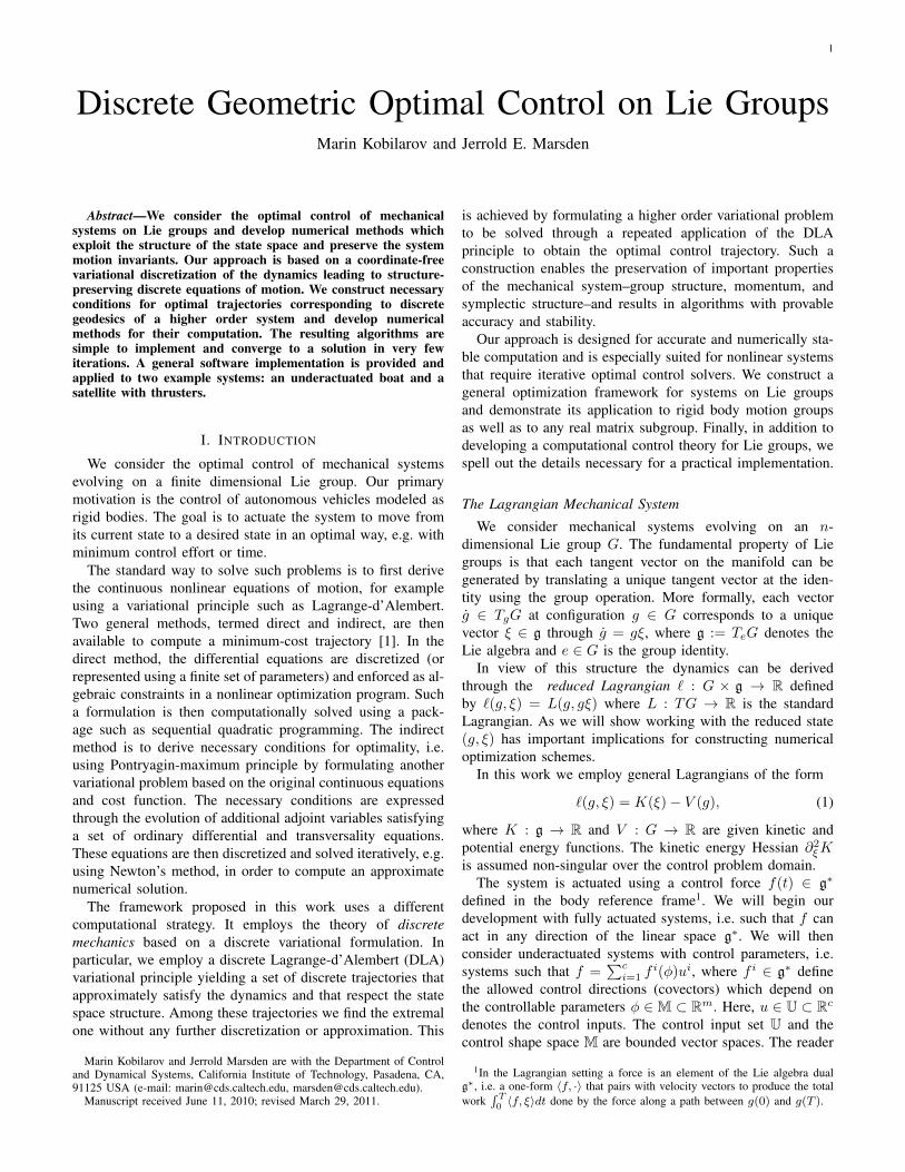
A trajectory is represented numerically using a set of N+1equally spaced in time points denoted g0:N := {g0, ..., gN},where gk ≈ g(kh) ∈ G and h = T/N denotes the time-step. The section between each pair of points gk and gk+1

is interpolated by a short curve that must lie on the manifold(Fig. 1). The simplest way to construct such a curve is througha map τ : τ : g → G and Lie algebra element ξk ∈ g suchthat ξk = τ−1(g−1k gk+1)/h. The map is defined as follows.

Definition III.1. The retraction map τ : g → G is a C2-diffeomorphism around the origin such that τ(0) = e. It is usedto express small discrete changes in the group configurationthrough unique Lie algebra elements.

2ad∗ξ µ is defined by 〈ad∗ξ µ, η〉 = 〈µ, adξ η〉, for some η ∈ g.

Thus, if ξk were regarded as an average velocity betweengk and gk+1 then τ is an approximation to the integral flow ofthe dynamics. The important point, from a numerical point ofview, is that the difference g−1k gk+1 ∈ G, which is an elementof a nonlinear space, can now be represented uniquely by thevector ξk in order to enable unconstrained optimization in thelinear space g for optimal control purposes.

G

gk−1

gk

gk+1

ξk = τ−1(g−1k gk+1)/hg

e

ξk

ξk−1

τ

τ

Fig. 1. A trajectory (solid) on the Lie group G discretized using a sequence ofarcs (dashed) represented by Lie algebra vectors ξk ∈ g through the retractionmap τ .

Next, we define the following operators related to τ .

Definition III.2. [11], [14] Given a map τ : g→ G, its right-trivialized tangent dτ ξ : g → g and its inverse dτ−1ξ : g → gare such that, for a some g = τ(ξ) ∈ G and η ∈ g, thefollowing holds

∂ξτ(ξ) · η = dτ ξ ·η · τ(ξ), (5)

∂ξτ−1(g) · η = dτ−1ξ · (η · τ(−ξ)) . (6)

Note that it can be shown by differentiating the expressionτ−1(τ(ξ)) = ξ that

dτ−1ξ · dτξ · η = η,

to confirm that these linear maps are indeed the inverse ofeach other.

Intuitively, after the derivative in the direction η is taken,i.e. ∂ξτ(ξ) · η, the resulting vector (at point τ(ξ)) is translatedback to the origin using right-multiplication by τ(−ξ) [14].In practice, as will be shown, these maps are easily derivedas n× n matrices. Finally, we require the tangent maps to benonsingular over the optimization domain, defined next.

Definition III.3. The optimization domain Dτ ⊂ g is aconnected open set containing the origin e ∈ g such that dτhξ(and dτ−1hξ ) are non-singular for every ξ ∈ Dτ .

The numerical algorithms proposed in the paper are re-stricted to operate over Dτ , i.e. the time-step h and velocitiesξk are chosen to satisfy hξk ∈ Dτ for all k = 0, ..., N − 1.

Retraction Map (τ ) Choices: a)The exponential mapexp : g → G, defined byexp(ξ) = γ(1), with γ : R → Gis the integral curve through theidentity of the vector field asso-ciated with ξ ∈ g (hence, withγ(0) = ξ). The right-trivialized derivative of the map exp

5

and its inverse are defined as

dexpx y =

∞∑j=0

1

(j + 1)!adjx y, (7a)

dexp−1x y =

∞∑j=0

Bjj!

adjx y, (7b)

where Bj are the Bernoulli numbers. Typically, these ex-pressions are truncated in order to achieve a desired orderof accuracy. The first few Bernoulli numbers are B0 = 1,B1 = −1/2, B2 = 1/6, B3 = 0 (see [8]).

b) The Cayley map cay : g → G is defined by cay(ξ) =(I−ξ/2)−1(I +ξ/2) and is valid for a general class forquadratic groups that include the groups of interest in thepaper. Based on this simple form, the derivative maps become([8], §IV.8.3)

dcayx y =(e− x

2

)−1y(e+

x

2

)−1, (8a)

dcay−1x y =(e− x

2

)y(e+

x

2

). (8b)

The third choice is to use canonical coordinates of the secondkind (ccsk) [8] which are based on the exponential map andare not considered in this paper.

C. Discrete Variational Formulation

With a discrete trajectory in place we follow the approachtaken in [10], [9] in order to construct a structure-preserving(i.e. group, momentum, and symplectic) integrator of the dy-namics. We make a simple extension to include potential andcontrol forces through a trapezoidal quadrature approximation.In particular, the action in (3) is approximated along eachdiscrete segment between points gk and gk+1 through∫ (k+1)h

kh

[K(ξ)−V (g)]dt≈h[K(ξk)− V (gk)+V (gk+1)

2

], (9a)∫ (k+1)h

kh

〈f, g−1δg〉≈ h2

[〈fk, g−1k δgk〉+〈fk+1, g−1k+1δgk+1〉

]. (9b)

Variations of Lie algebra elements are related to variationson the group through the following expression which may beobtained through differentiation and application of (6),

δξk = δτ−1(g−1k gk+1)/h = dτ−1hξk(−ηk + Adτ(hξk) ηk+1)/h,

where ηk = g−1k δgk. The operator Adg : g → g can beregarded as a change of basis with respect to the argumentg ∈ G (see [3], [35]) and is defined by

Adg ξ = gξg−1.

The discrete variational principle which will form the basisfor our discrete optimal control framework can now be stated.The following result is a straightforward extension from [10],[9]. The only difference is that we consider Lagrangians ofthe form (1) and employ a trapezoidal discretization:

Proposition 1. A mechanical system on Lie group G withkinetic energy K, potential energy V , subject to forces f ,satisfies the following equivalent conditions:

1. The discrete reduced Lagrange-d’Alembert principle holds

δ

N−1∑k=0

[K(ξk)− V (gk) + V (gk+1)

2

]

+

N−1∑k=0

1

2

[〈fk, g−1k δgk〉+ 〈fk+1, g

−1k+1δgk+1〉

]= 0,

(10)

where ξk = τ−1(g−1k gk+1)/h.2. The discrete reduced Euler-Poincare equations of motion

hold

µk −Ad∗τ(hξk−1)µk−1 = h (−g∗k∂gV (gk) + fk) , (11a)

µk = (dτ−1hξk)∗∂ξK(ξk), (11b)

gk+1 = gkτ(hξk). (11c)

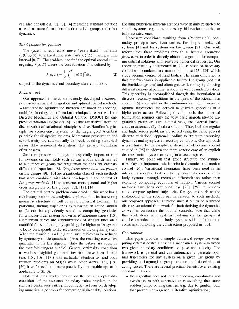
Equations (11) can be considered as a discrete approx-imation to (4). The discrete Euler-Poincare equation (11a)corresponds to (4a). Eq. (11b) is the discrete Legendre trans-form corresponding to (4b), while (11c) is the discretereconstruction analogous to (4c). These equations can be usedto compute the next velocity and group elements ξk, and gk+1,respectively, given the previous elements ξk−1 and gk. Fig. 2gives a more geometric explanation of the update (11a).

(dτ−1hξk−1

)∗

∂ξK(ξk−1)

(dτ−1hξk

)∗µk−1

µk

Ad∗τ(hξk−1)µk−1Ad∗τ(hξk−1)

hfk

gkgk−1

gk+1

∂ξK(ξk)

move to next

point by change

of basismove to point atstart of segment

Fig. 2. The discrete covariant version of the Euler-Poincare equation µ −ad∗ξ µ = f , where µ = ∂ξK(ξ). The discrete momentum µk at point kis obtained using the right trivialized tangent (dτ−1

hξk)∗ which brings the

derivative ∂ξK(ξk) to the body-fixed basis at gk . The momentum evolutionis then expressed through the difference of µk−1 and µk , i.e. by transformingµk−1 in that same basis at gk through the Ad∗ map where proper vectorsubtraction can be applied. The resulting change is caused by forces hfk (theeffects of potential V are omitted for clarity). Note that all vectors shown areelements of g∗ and are shown above the group configuration only to illustratethe basis with respect to which they are defined.

Boundary Conditions: While the discrete configurationsgk and forces fk approximate their continuous counterpartsat times t = kh, we still have not established the exactrelationship between the discrete and continuous momenta,µk and µ(t) = ∂ξK(ξ(t)), respectively. This is particularlyimportant for properly enforcing boundary conditions thatare given in terms of continuous quantities. The followingequations (12a) and (12b) relate the momenta at the initialand final times t = 0 and t = T and are used to transformbetween the continuous and discrete representation:

µ0 − ∂ξK(ξ(0)) =h

2(g∗0∂gV (g0) + f0) , (12a)

∂ξK(ξ(T ))−Ad∗τ(hξN−1)µN−1 =h

2(g∗N∂gV(gN )+fN ) . (12b)

These equations can also be regarded as structure-preservingvelocity boundary conditions for given fixed velocities ξ(0)

6

and ξ(T ). They follow from properly enforcing energy balanceat the boundaries, achieved by adding the momentum changeterm 〈µ(T ), g−1N δgN 〉 − 〈µ(0), g−10 δg0〉 to the discrete actionin the principle (10).

The exact form of (11) and (12) depends on the choice ofτ . It is important to point out that this choice will influencethe computational efficiency of the optimization frameworkwhen the equalities above are enforced as constraints. We havespecified two basic choices, τ = exp (7a) and τ = cay (8a)for their ease of implementation and run-time efficiency.

D. Preservation Properties

One of the main benefits of employing the variationalnumerical framework lies in its preservation properties, sum-marized by the following theorems.

Theorem III.4. [9] The discrete flow (11) preserves thediscrete symplectic form, expressed in coordinates as

ω` =∂2`(gk, τ

−1(g−1k gk+1)/h)

∂gik∂gjk+1

dgik ∧ dgjk+1,

where ∧ is the standard wedge product between differentialforms [35]. The symplectic form can also be written as thedifferential of the canonical one-form θ` with ω` = dθ` where

θ` · δgk =

⟨− 1

hµk − g∗k∂gV(gk), g−1k δgk

⟩.

The symplectic form is physically related to the phase spacestructure. Its preservation during integration, for instance,signifies that a volume of initial conditions would not be spu-riously inflated or deflated due to numerical approximations.Volume preservation means that the orbits of the dynamics willhave a predictable character and no artificial damping normallyemployed by Runge-Kutta methods is needed to stabilize thesystem [7].

Theorem III.5. [9], [14] The discrete dynamics (11) pre-serves the momentum. In particular, in the absence of potentialand non-conservative forces, the update scheme preserves thediscrete spatial momentum map J : G× g→ g,

J(gk, ξk) · v = Ad∗g−1kµk · v,

for any v ∈ g; or equivalently J(ga, ξa) = J(gb, ξb), for anytime indices a, b.

Practically speaking, whenever the continuous system pre-serves momentum, so does the discrete. Any change in themomentum then exactly reflects the work done by non-conservative forces. Such a momentum-symplectic schemealso exhibits long-term stable energy behavior close to the truesystem energy [7]. Another property carried over to continuouscase is time-scaling.

Remark 1. Order of Accuracy. The order of accuracy of thedynamics update depends on the accuracy of the Lagrangianapproximation. Since the trapezoidal approximations (9a) and(9b) are second-order accurate then it can be shown (see[7]) that the discrete equations (11) are also of second orderaccuracy. The trapezoidal rule was chosen since it provides

the simplest second-order scheme. Higher-order methods byproper choice of the Lagrangian, termed symplectic Runge-Kutta (see [8], [12], [14]), are possible but not considered inthis work.

Remark 2. Time-scaling preservation. The trajectory g0:N ,ξ0:N−1 with time-step h satisfies the discrete dynamics (11)subject to forces f0:N if and only if the trajectory g0:N ,{ξ0/s, ..., ξN−1/s} with time-step h′ = sh, subject to forces{f0/s2, ..., fN/s2} satisfies the discrete dynamics, for a givenscalar s > 0.

Finally, the group structure is exactly preserved since thetrajectory g0:N is reconstructed from the discrete velocityξ0:N−1 using the map τ which by definition maps to thegroup (11c). This avoids issues with dissipation and numericaldrift associated with reprojection used in other methods,e.g. in methods based on matrix orthogonality constraints orquaternions.

IV. FULLY ACTUATED SYSTEMS

We first develop the simplest case with a mechanical kineticenergy

K(ξ) =1

2〈Iξ, ξ〉,

with full unconstrained actuation, without potential or externalforces and without any velocity constraints. The map I : g→g∗ is called the inertia tensor and is assumed full rank. Sincethere is full control over f the control effort cost function (2)can be expressed as J(f) =

∫12‖f(t)‖2dt. It is approximated

through trapezoidal quadrature, analogously to (10), using thesummation

J(f) ≈N−1∑k=0

h

4

(‖fk‖2 + ‖fk+1‖2

). (13)

The optimal control problem for the system (11) with givenfixed initial and final states (g(0), ξ(0)) and (g(T ), ξ(T ))respectively can be stated as

Compute: ξ0:N−1, f0:N

minimizingN−1∑k=0

h

4

(‖fk‖2 + ‖fk+1‖2

)subject to:

µ0 − I ξ(0) = (h/2)f0,

µk −Ad∗τ(hξk−1)µk−1 = hfk, k = 1, ..., N − 1,

I ξ(T )−Ad∗τ(hξN−1) µN−1 = (h/2)fN ,

µk = (dτ−1hξk)∗ I ξk,g0 = g(0),

gk+1 = gkτ(hξk), k = 0, ..., N − 1,

τ−1(g−1N g(T )) = 0.

(14)

The constraints follow directly from the discrete mechan-ics (11), boundary conditions (12), and by noting that ∂ξK =Iξ. The last equation ensures that the difference between thegiven and reconstructed configurations is zero.

7

A. Optimality Conditions

Trajectories satisfying the constrained nonlinear optimiza-tion problem (14) are computed through the derivation ofoptimality conditions stated in the following proposition.

Proposition 2. The trajectory of a discrete mechanical sys-tem on a Lie group G with algebra g and Lagrangian`(ξ) = 1

2 〈I ξ, ξ〉 with fixed initial and final configurations andvelocities (g(0), ξ(0)) ∈ G × g and (g(T ), ξ(T )) ∈ G × gminimizes the total control effort only if the discrete body-fixed velocity curve ξ0:N−1 satisfies the following conditions:

Necessary Conditions for Optimality

νk −Ad∗τ(hξk−1)νk−1 = 0, k = 1, ..., N − 1 (15a)

τ−1(τ(hξ0) · · · τ(hξN−1) · (g(0)−1g(T ))−1) = 0, (15b)where:

νk=(dτ−1hξk)∗∂ξK(λ0:N ,k)(ξk), (15c)

K(λ0:N,k)(ξk)=〈(dτ−1hξk)∗Iξk, λk−Adτ(hξk)λk+1〉/h, (15d)

λ[0 =2 (µ0−I ξ(0)) /h, (15e)

λ[k=(µk−Ad∗τ(hξk−1)

µk−1)/h, k=1, ..., N−1 (15f)

λ[N =2(I ξ(T )−Ad∗τ(hξN−1) µN−1

)/h, (15g)

µk=(dτ−1hξk)∗ Iξk. (15h)

Note: The proposition defines Nn equations (15a)-(15b) inthe Nn unknowns ξ0, ..., ξN−1. A solution can be found usingnonlinear root finding.

Proof: Define the discrete action S according to

S(ξ0:N−1, f0:N , λ0:N )

= 〈µ0 − Iξ(0)− hf0/2, λ0〉

+

N−1∑k=1

〈µk −Ad∗τ(hξk−1)µk−1 − hfk, λk〉

+ 〈Iξ(T )−Ad∗τ(hξN−1) µN−1 − hfN/2, λN 〉

+

N−1∑k=0

h

4

(‖fk‖2 + ‖fk+1‖2

), (16)

where µk = (dτ−1hξk)∗ Iξk should be regarded as a function ofξk. Taking variations δS with respect to fk and λk we obtain3

λ[k = fk = (µk −Ad∗τ(hξk−1)µk−1)/h.

Next, freeze the adjoint trajectory λ0:N and define the func-tions K(λ0:N ,k) : g→ R, for k = 0, ..., N − 1 by

K(λ0:N ,k)(ξ) = 〈(dτ−1hξ )∗ Iξ, λk −Adτ(hξ) λk+1〉/h. (17)

The ξ-dependent discrete action along fixed λ0:N can berewritten as

Sλ0:N(ξ0:N−1) = h

N−1∑k=0

K(λ0:N ,k)(ξk).

3The superscript operators [ : g → g∗ (flat) and ] : g∗ → g (sharp)are used to convert between vector fields and their duals (one-forms). Underidentification g ∼ Rn, [ can simply be regarded as converting a column vectorinto a row vector, and ] as the opposite operation [35].

For less cluttered notation the shorthand expression

K(ξk) := K(λ0:N ,k)(ξk), (18)

will also be employed since the index k in K(λ0:N ,k) becomesclear from the argument ξk. The point is that λ in (17) shouldbe regarded as fixed, i.e. not dependent on ξ. The optimalityconditions can now be regarded as a set of equations satisfyingthe dynamics of another higher order discrete Hamiltoniansystem with discrete Lagrangian L = K throughδSλ0:N

(ξ0:N−1) = 0 ⇐⇒ νk −Ad∗τ(hξk−1)νk−1 = 0, (19)

where νk = (dτ−1hξk)∗∂ξK(ξk) ∈ g∗ is a momentum-likequantity for the system with Lagrangian L. The relation (19)is nothing but the discrete Euler-Poincare equation of thisnew system and was obtained in the same way the standarddynamics update (11a) followed from the principle (10). Thiskey insight leads directly to a convenient numerical schemefor computing the optimal controls.

The final configuration gN is computed by reconstructingthe curve from the velocities ξ0:N−1 and the boundary condi-tion gN = g(T ) is enforced through the relation (15b) withoutthe need to optimize over any of the configurations gk.

We point out the resulting formulation does not requireoptimizing over additional Lagrange multiplier variables. Ithas the minimum possible problem dimension and avoidsconvergence and instability issues due to improper multiplierinitialization.

B. Implementing the Necessary Conditions.

An optimal trajectory is computed as the root of equa-tions (15a)-(15b). Their exact form depends on the momentumexpression (15c) which can be computed numerically usingfinite differences, e.g. using:

〈νk, η〉 (20)

≈ 1

2ε

[K(λ0:N ,k)(ξk+εdτ−1hξkη)−K(λ0:N ,k)(ξk−ε dτ−1hξkη)

],

along basis elements η ∈ g with a small ε > 0. In otherwords, the components of νk with respect to a chosen Liealgebra basis {ei} are computed according to νik = 〈νk, ei〉for any Lie group G.

Alternatively, the momentum can be expressed in closedform by differentiating the kinetic energy K to obtain〈νk, η〉= 〈(∂ξdτ−1hξk ·dτ

−1hξk

η)∗ I ξk,∆λk〉+ 〈(dτ−1hξk)

∗ I(dτ−1hξk)∆λk + h ad∗Adτ(hξk)λk+1µk, η〉,

(21)

where ∆λk = λk−Adτ(hξk) λk+1. Expression (21) is derivedusing straightforward differentiation (one can also consult [22]for more details) and using A.1. One can choose to implementthe necessary conditions using either (20) or (21).

V. UNDERACTUATED SYSTEMS WITH CONTROLPARAMETERS

We next extend the system dynamics to include non-trivialactuation and position dependent forces. Assume that the con-trol forces are applied along body-fixed directions defined by

8

the control covectors {f1(φ), ..., f c(φ)}, c ≤ n, f i : M→ g∗

which depend on control parameters φ : [0, T ] → M. Theseextra parameters can be regarded as the shape variables of thecontrol basis, i.e. parameters that do not affect the inertialproperties of the systems but which determine the controldirections. Assume that the system is controlled using controlinput u : [0, T ] → U applied with respect to the basis{f i(φ)}. In addition, assume that the system is subject toconfiguration-dependent forces collectively represented by thefunction fconf : G → g∗ and dissipative velocity-dependentforces fvel : g → g∗. For instance, forces arising from thepotential V take the form fconf(g) = −g∗∂gV (g). while simpleviscous resistance or linear drag forces can be expressed asfvel(ξ) = −Dξ, where D is damping positive definite map.

The total force acting in the body frame can then beexpressed as the sum of the control and external forcesaccording to

f(g, ξ) =

c∑i=1

uif i(φ) + fconf(g) + fvel(ξ).

In this problem the control effort to be minimized is expressedas∫ T0

12‖u(t)‖2dt.

Dissipative Force discretization: In our frameworkvelocity-dependent forces fvel(ξk) are defined over the k-th segment, and have no clear meaning over a particularpoint. The contribution of such forces at a particular pointcan be specified by assuming the following virtual workapproximation

∫ (k+1)h

kh

fvel(ξ) ·η(t)≈ h2〈(dτ−1hξk)

∗fvel(ξk), ηk+Adτ(hξN)ηk+1〉,

where η = g−1δg denotes the usual Lie group variations. Suchdiscretization is motivated by the way variations contribute toHamilton’s principle discretization (10)

δ

(∫ (k+1)h

kh

`(ξ)dt

)·η≈h〈(dτ−1hξk)

∗∂ξ`(ξk),−ηk+Adτ(hξN)ηk+1〉,

where the left and right variations are averaged instead ofsubtracted. Fig. 2 also helps explain how vectors defined alonga segment transform to its start and end points.

The necessary conditions for an optimal trajectory aredefined in the following proposition (which extends Prop. 2).

Proposition 3. A discrete mechanical system with kinetic en-ergy K(ξ) and control input directions f i(φ) subject to config-uration and dissipative forces fconf(g) and fvel(ξ), respectively,moves with minimum control effort between fixed initial andfinal states (g(0), ξ(0)) ∈ G× g, ((g(T ), ξ(T )) ∈ G× g, onlyif the discrete velocity curve ξ0:N−1, control parameters φ0:N ,and adjoint variables λ0:N satisfy the following conditions:

Necessary Conditions for Optimality

νk−Ad∗τ(hξk−1)νk−1 =−hg∗k∂g〈fconf(gk),λk〉,

k = 1, ..., N−1(22a)

τ−1(g−1N g(T )) = 0, (22b)

µ0−I ξ(0) = (h/2)f+0 , (22c)

µk−Ad∗τ(hξk−1)µk−1 =(h/2)(f−k +f+k ), k=1, ..., N−1 (22d)

I ξ(T )−Ad∗τ(hξN−1) µN−1 =(h/2)f−N , (22e)c∑i=1

uik(∂φf

i(φk)])λk = 0, k = 0, ..., N (22f)

where νk ∈ g∗, f±k ∈ g∗, uk ∈ U are defined by

νk = (dτ−1hξk)∗∂ξKλ0:N ,k(ξk), (22g)

Kλ0:N ,k(ξk) = 〈(dτ−1hξk)∗Iξk, λk −Adτ(hξk) λk+1〉/h

− 1

2〈(dτ−1hξk)∗fvel(ξk), λk+Adτ(hξk)λk+1〉,

f−k =c∑i=1

uikfi(φk) + fconf(gk) + (dτ−1−hξk−1

)∗fvel(ξk−1),

f+k =

c∑i=1

uikfi(φk) + fconf(gk) + (dτ−1hξk)∗fvel(ξk),

uik = 〈f i(φk), λk〉, (22h)g0 = g(0), (22i)gk+1 = gkτ(hξk), (22j)

Note: The proposition defines (Nn+ (N + 1)n+ (N + 1)m)equations (22a)-(22f) in the (Nn + (N + 1)n + (N + 1)m)unknowns (ξ0:N−1, λ0:N , φ0:N ). A solution can be found usingstandard nonlinear root finding. When the control basis is con-stant (i.e. m = 0) then the optimization is over (ξ0:N−1, λ0:N )only; f i(φk) should be replaced with f i and (22f) is omitted.

Proof: Define the discrete action S similarly to (16)according to

S(ξ0:N−1, u0:N , φ0:N , λ0:N ) =

〈µ0 − Iξ(0)− (h/2)f+0 , λ0〉

+

N−1∑k=1

〈µk−Ad∗τ(hξk−1)µk−1−(h/2)(f−k +f+k ), λk〉

+ 〈Iξ(T )−Ad∗τ(hξN−1) µN−1−(h/2)f−N , λN 〉

+

N−1∑k=0

h

4

(‖uk‖2 + ‖uk+1‖2

),

(23)

where we used the shorthand notation

f−k =

c∑i=1

uikfi(φk) + fconf(gk) + (dτ−1−hξk−1

)∗fvel(ξk−1),

f+k =

c∑i=1

uikfi(φk) + fconf(gk) + (dτ−1hξk)∗fvel(ξk).

Analogously to the fully actuated case (17), keep themultiplier trajectory λ0:N frozen and define the function

9

K(λ0:N ,k) : g→ R by

K(λ0:N ,k)(ξ) =〈(dτ−1hξ )∗Iξ, λk −Adτ(hξ) λk+1〉/h

− 1

2〈(dτ−1hξ)∗fvel(ξ), λk+Adτ(hξ)λk+1〉.

(24)

In addition, define the function V(λ0:N ,k) : G→ R by

V(λ0:N ,k)(g) = 〈fconf(g), λk〉.Similarly to (18) assume that following shorthand notation

K(ξk) := K(λ0:N ,k)(ξk), V(gk) := V(λ0:N ,k)(gk).

As the naming suggests, K and V play the role of kinetic andpotential energies for the higher order system whose dynamicswill determine the optimality conditions. The ξ-dependent partof the action (23) can be expressed, along fixed λ0:N , by

Sλ0:N(ξ0:K)=h

N−1∑k=0

(K(ξk)− 1

2[V(gk) +V(gk+1)]

). (25)

Note that the action (23) was expressed in terms of eachK(ξk) (24) by combining all terms in S containing ξk andusing the identity

(dτ−1−hξk)∗fvel(ξk) = Ad∗τ(hξk)(dτ−1hξk

)∗fvel(ξk)

which follows from A.3.After extremizing this action, it immediately follows from

the general discrete Lagrange-d’Alembert principle (Prop. 1)that

νk −Ad∗τ(hξk−1)νk−1 = −hg∗k∂gV(gk), (26)

where νk = (dτ−1hξk)∗∂ξK(ξk) ∈ g∗ is a momentum-like quan-tity for the higher-order system with Lagrangian L = K − V .In summary, the relation (22a) follows from applying thevariational equations (10) to the action Sλ0:N

.Eqs. (22c)-(22e) enforce the dynamics after taking varia-

tions δλk, i.e.

δλ0 ⇒ µ0−I ξ(0) = (h/2)f+0 ,

δλk ⇒ µk−Ad∗τ(hξk−1)µk−1 =(h/2)(f−k +f+k ),

δλN ⇒ I ξ(T )−Ad∗τ(hξN−1) µN−1 =(h/2)f−N .

Variations of the parameters φk result in

δφk ⇒⟨

c∑i=1

uik∂φfi(φk), λk

⟩= 0, for k = 0, ..., N,

which can be rewritten as the relation (22f). In the specialcase when the control input basis elements f i are constant, therelation (22f) vanishes. Variations with respect to the controlsδuk result in

δuik ⇒ −〈f i(φk), λk〉+ uik = 0, for k = 0, ..., N,

from which the controls uk can be computed in terms of themultipliers (included as condition (22h)). Since the controlsu0:N can be computed internally it is not necessary to includethem as part of the optimization variables in Prop. 3.

The remaining equations are identical to the ones derived inProp. 2. Note that the optimization is not performed over theconfigurations gk, since they can be internally reconstructedaccording to (22i)-(22j).

Vector-matrix Form.: The term on the right hand sideof (22a) can be better understood under the identification g ∼Rn by treating g as a matrix and all other variables as columnvectors. In this case g∗∂g〈fconf(g), λ〉 = gT (∂gfconf(g))Tλ.Similarly, the expression in (22f) should be understood as(∂φf

i(φ)])λ = ∂φf

i(φ)Tλ.Example: constant force field.: The force (22a) has a

closed form whenever the external force is constant in theglobal frame, i.e. when it can be written as fconf(g) =Ad∗g fconst. Typical examples of such forces are gravity (onthe surface of the Earth) or a simple model of wind blowingin a constant direction. Using A.1 the expression becomes

g∗∂g〈fconf(g), λ〉 = − ad∗λ Ad∗g fconst = − ad∗λ fconf(g).

Corollary 1. The optimality conditions in Prop. 2 and 3preserve the higher order discrete symplectic form ωL = dθLwhere the canonical one-form θL is given by

θL · δgk =

⟨− 1

hνk − g∗k∂gV(gk), g−1k δgk

⟩.

The claim follows directly from Thm. III.4.

Controllability Issues

In the fully actuated case §IV, gradient-based methodsare always guaranteed to find a (local) optimum since theconstraints are linearly independent. This is not the case withunderactuation since controllability is generally not guaran-teed. In the discrete setting, lack of controllability appearsas a singularity of the optimality conditions which obstructsiterative optimization. This is an issue with any numericalmethod for solving optimal optimal control problems forconstrained systems. In that respect our proposed approachis no better than any other standard nonlinear programmingtechnique. Yet, there appears to be an interesting connectionbetween the standard, i.e. continuous, controllability and itscounterpart in our proposed discrete setting. This link is brieflyexplored next with further development left for future work.

A standard way to define controllability for the type ofsystems considered in this paper is through the symmetricproduct, denoted 〈· : ·〉 : g× g→ g and defined by

〈ξ : η〉 = −I−1(ad∗ξ Iη + ad∗η Iξ

).

In the continuous setting, iterated symmetric products of theinput vector fields bi = I−1f i determine which velocitiescan be reached while iterated Lie brackets of these reachablevelocities determine which configurations are achievable. Inparticular, exact controllability tests are directly computableassuming the system starts and ends with zero velocity [36].A similar general claim can be made regarding our discretesetting for N → ∞ since the discrete dynamics approachesthe continuous one. However, such a claim is not useful inpractice since a realistically implementable algorithm is basedon a small N .

In that respect, there is an interesting link between thestandard continuous and the required discrete controllabilityconditions. More specifically, the discrete dynamics (22d) can

10

be expressed (after setting τ = exp and ignoring externalforces) as∞∑i=0

Bii!2i

(〈ξk :i ξk〉 − (−1)i〈ξk−1 :i ξk−1〉

)= huib

i (27)

where 〈ξ :i ξ〉 denotes taking the product using the firstargument recursively i times. In addition, the reconstructioncondition (22b) can be expressed through the Baker-Campbell-Hausdorff formula [4] as

τ−1(τ(hξ0)· · ·τ(hξN−1))=h

N−1∑k=0

ξk+h2

2

N−1∑i,j=0

[ξi, ξj ]+hot, (28)

where “hot” denotes higher-order terms of iterated Lie brack-ets. Note that if the closure under Lie algebra bracket operation[·, ·], denoted Lie(ξ0:N−1), spans all possible directions ofmotions then (28) ensures that any final configuration g(T )can be reached from any starting configuration g(0). Thiscorresponds exactly to the continuous controllability conditionrequiring that the Lie algebra closure of achievable velocitieshas full rank [4]. Note that this similarity applies in the contextof kinematic systems since the discrete composition of flowsin (28) can be regarded as a curve generated by a kinematicallyreduced continuous system.

It would be interesting to define more precisely the notionof discrete controllability through (27) and (28). This willenable the algorithm to determine not only whether a state isreachable but also an appropriate number of discrete segmentsN required to reach it. As a rule of thumb, any practicalimplementation should have N ≥ 2 + n, where n = dim(G),to account for the two boundary conditions on velocities andto provide at least n discrete flows.

VI. APPLICATIONS TO MATRIX GROUPS

We now specify the operators required to implement Prop. 2and Prop. 3 for typical rigid body motion groups and generalreal matrix subgroups. While we have given more than onegeneral choice for τ , for computational efficiency we rec-ommend the Cayley map since it is simple and does notinvolve trigonometric functions. In addition, it is suitablefor iterative integration and optimization problems since itsderivatives do not have any singularities that might otherwisecause difficulties for gradient-based methods.

A. SO(3)

The group of rigid body rotations is represented by 3-by-3matrices with orthonormal column vectors corresponding tothe axes of a right-handed frame attached at the body. Definethe map · : R3 → so(3) by

ω =

0 −w3 w3

w3 0 −w1

−w2 w1 0

. (29)

A Lie algebra basis for SO(3) can be constructed as{e1, e2, e3}, ei ∈ so(3) where {e1, e2, e3} is the standardbasis for R3. Elements ξ ∈ so(3) can be identified with thevector ω ∈ R3 through ξ = ωαeα, or ξ = ω. Under such

identification the Lie bracket coincides with the standard crossproduct, i.e. adω ρ = ω × ρ, for some ρ ∈ R3. Using thisidentification we have

cay(ω) = I3 +4

4 + ‖ω‖2(ω +

ω2

2

). (30)

The linear maps dτ ξ and dτ−1ξ are expressed as the 3 × 3matrices

dcayω=2

4+‖ω‖2 (2I3+ω) , dcay−1ω =I3−ω

2+ωωT

4. (31)

We point out that with the choice τ = cay the optimizationdomain is not restricted, i.e. Dcay = g since the maps (31)are non-singular for any ξ ∈ g. This is not the case for theexponential map for which Dexp = {ξ ∈ g | ‖ξ‖ < 2π/h}since the exponential map derivative is singular whenever thenorm of its argument is a multiple of 2π [8], and the originrequires special handling.

B. SE(2)

The coordinates of SE(2) are (θ, x, y) with matrix repre-sentation g ∈ SE(2) given by:

g =

cos θ − sin θ xsin θ cos θ y

0 0 1

. (32)

Using the isomorphic map · : R3 → se(2) given by:

v =

0 −v1 v2

v1 0 v3

0 0 0

for v =

v1v2v3

∈ R3,

{e1, e2, e3} can be used as a basis for se(2), where {e1, e2, e3}is the standard basis of R3.

The map τ : se(2)→ SE(2) is given by

cay(v)=

14+(v1)2

[(v1)2−4 −4v1 −2v1v3+4v2

4v1 (v1)2−4 2v1v2+4v3

]0 0 1

,while the map [dτ−1ξ ] becomes the 3x3 matrix:

[dcay−1v ] = I3 −1

2[adv] +

1

4

[v1 · v 03×2

], (33)

where

[adv] =

0 0 0v3 0 −v1−v2 v1 0

.C. SE(3)

We make the identification SE(3) ≈ SO(3) × R3 usingelements R ∈ SO(3) and x ∈ R3 through

g =

[R x0 1

], g−1 =

[RT −RTx0 1

].

Elements of the Lie algebra ξ ∈ se(3) are identified withbody-fixed angular and linear velocities denoted ω ∈ R3 andv ∈ R3, respectively, through

ξ =

[ω v0 0

],

11

where the map · : R3 → so(3) is defined in (29).Using this identification we have

τ(ξ) =

[τ(hωk) hdτhωk vk

0 1

],

where τ : so(3) → SO(3) is given by (30) and dτω : R3 →R3 by (31).

The matrix representation of the right-trivialized tangentinverse dτ−1(ω,v) : R3 × R3 → R3 × R3 becomes

[dcay−1(ω,v)] =

[I3 − 1

2 ω + 14ωω

T 03

− 12

(I3 − 1

2 ω)v I3 − 1

2 ω

]. (34)

D. General matrix subgroups

The Lie algebra of a matrix Lie group coincides with theone-parameter subgroup generators of the group. Assume thatwe are given a k-dimensional Lie subalgebra denoted g ⊂gl(n,R). It is isomorphic to the space of generators of a uniqueconnected k-dimensional matrix subgroup G ⊂ GL(n,R).Therefore, a subalgebra g determines the subgroup G in aone-to-one fashion:

g ⊂ gl(n,R)⇐⇒ G ⊂ GL(n,R).

The two ingredients necessary to convert the necessary condi-tions in Prop. (2) into algebraic equalities are: a choice of basisfor g; and an appropriate choice of inner product (metric).

Assume that the Lie algebra basis elements are {Eα}kα=1,Eα ∈ g, i.e. that every element ξ ∈ g can be written as ξ =ξαEα. Define the following inner product for any ξ, η ∈ g

〈〈ξ, η〉〉 = tr(BξT η),

where B is an n × n matrix such that 〈〈Eα, Eβ〉〉 = δβα andtr is the matrix trace. Correspondingly, a pairing between anyµ ∈ g∗ and ξ ∈ g can be defined by

〈µ, ξ〉 = tr(Bµξ),

since the dual basis for g∗ is {[Eα]T }kα=1 in matrix form.Example: If g = so(3) then setting B =

diag(1/2, 1/2, 1/2) yields the standard inner product underthe identification so(3 ∼ R3, i.e. 〈µ, ξ〉 = µαξ

α.Example: If g = se(3) with basis then setting B =

diag(1/2, 1/2, 1/2, 1) the pairing yields the standard innerproduct if we identify se(3) with R3 × R3.

Kinetic Energy-Type Metric: After having defined a met-ric pairing, a kinetic energy operator I can be be expressedas

〈I(ξ), η〉 = tr(BIdξT η),

for some symmetric matrix Id ∈ GL(n,R).Example: Consider a rigid body on SO(3) with moments

of inertia J1, J2, J3 and Lagrangian `(ξ) = 12Jiξ

2i where the

ξi are the velocity components in the Lie algebra basis definedin §VI-A. The matrix Id must have the form

Id = diag(−J1+J2+J3,−J2+J1+J3,−J3+J1+J2)

Example: Consider a rigid body on SE(3) with princi-pal moments of inertia J1, J2, J3, mass m, and Lagrangian`(ω, v) = 1

2

(Jiω

2i +mvT v

), where (ω, v) ∈ (R3 × R3) ∼

se(3) are the body-fixed angular and linear velocities usingthe identification defined in §VI-C. The Lagrangian in thiscase can be equivalently expressed as `(ξ) = 1

2 tr(BIdξT ξ),

where ξ ∈ se(3) and

Id = diag(−J1+J2+J3,−J2+J1+J3,−J3+J1+J2,m).

With these definitions the optimality conditions in Prop. 2can be implemented for any given linear group by choosingB, Id and setting the inner product to the matrix trace. Fornumerical efficiency though, it is always preferable to employan identification with a vector space where a standard dotproduct is used.

VII. EXAMPLES

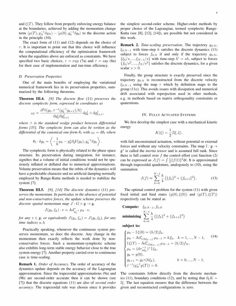
v

v⊥

ω

c

damping

windthrust

z

x

y

thrusters firing

sensor

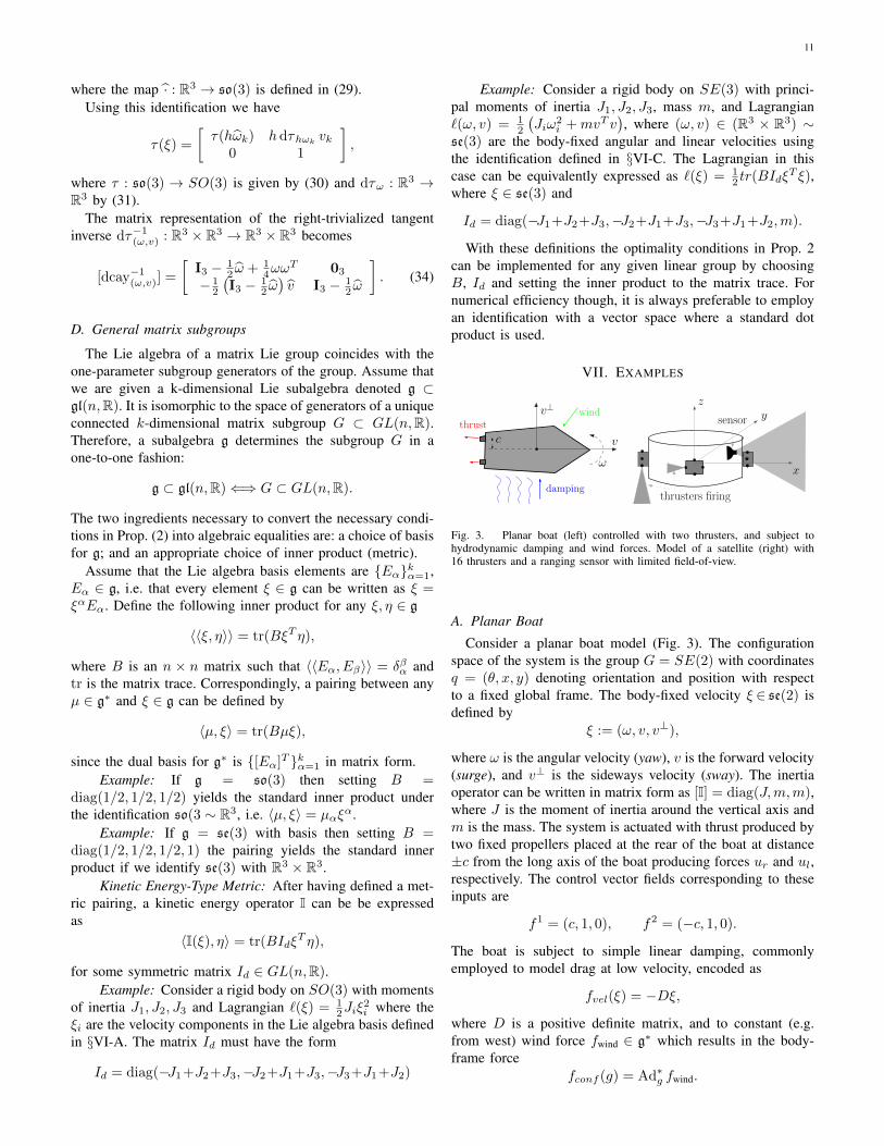
Fig. 3. Planar boat (left) controlled with two thrusters, and subject tohydrodynamic damping and wind forces. Model of a satellite (right) with16 thrusters and a ranging sensor with limited field-of-view.

A. Planar Boat

Consider a planar boat model (Fig. 3). The configurationspace of the system is the group G = SE(2) with coordinatesq = (θ, x, y) denoting orientation and position with respectto a fixed global frame. The body-fixed velocity ξ ∈ se(2) isdefined by

ξ := (ω, v, v⊥),

where ω is the angular velocity (yaw), v is the forward velocity(surge), and v⊥ is the sideways velocity (sway). The inertiaoperator can be written in matrix form as [I] = diag(J,m,m),where J is the moment of inertia around the vertical axis andm is the mass. The system is actuated with thrust produced bytwo fixed propellers placed at the rear of the boat at distance±c from the long axis of the boat producing forces ur and ul,respectively. The control vector fields corresponding to theseinputs are

f1 = (c, 1, 0), f2 = (−c, 1, 0).

The boat is subject to simple linear damping, commonlyemployed to model drag at low velocity, encoded as

fvel(ξ) = −Dξ,where D is a positive definite matrix, and to constant (e.g.from west) wind force fwind ∈ g∗ which results in the body-frame force

fconf (g) = Ad∗g fwind.

12

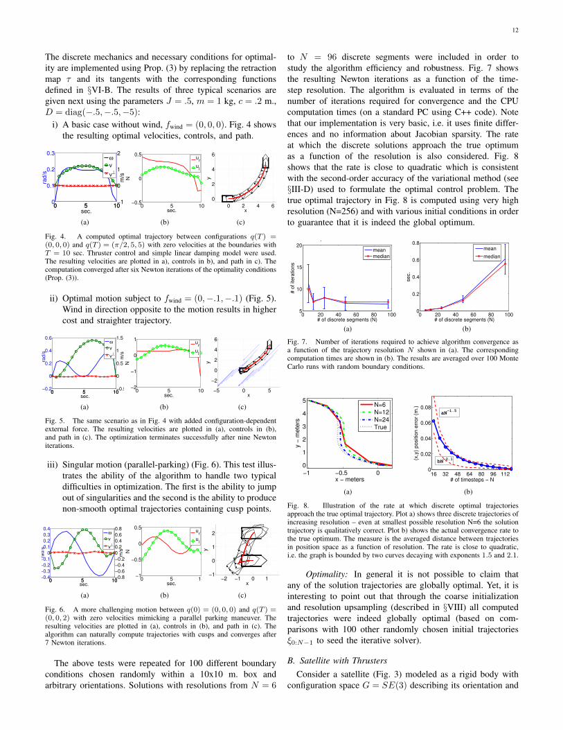
The discrete mechanics and necessary conditions for optimal-ity are implemented using Prop. (3) by replacing the retractionmap τ and its tangents with the corresponding functionsdefined in §VI-B. The results of three typical scenarios aregiven next using the parameters J = .5, m = 1 kg, c = .2 m.,D = diag(−.5,−.5,−5):

i) A basic case without wind, fwind = (0, 0, 0). Fig. 4 showsthe resulting optimal velocities, controls, and path.

0 5 100

0.1

0.2

0.3

rad/s

sec.

0 5 10−1

0

1

2

m/s

ω

v

v⊥

0 5 10−0.5

0

0.5

sec.

N

ur

ul

0 2 4 6

0

2

4

6

xy

(a) (b) (c)

Fig. 4. A computed optimal trajectory between configurations q(T ) =(0, 0, 0) and q(T ) = (π/2, 5, 5) with zero velocities at the boundaries withT = 10 sec. Thruster control and simple linear damping model were used.The resulting velocities are plotted in a), controls in b), and path in c). Thecomputation converged after six Newton iterations of the optimality conditions(Prop. (3)).

ii) Optimal motion subject to fwind = (0,−.1,−.1) (Fig. 5).Wind in direction opposite to the motion results in highercost and straighter trajectory.

0 5 10−0.2

0

0.2

0.4

0.6

rad

/s

sec.

0 5 10−0.5

0

0.5

1

1.5

m/s

ω

v

v⊥

0 5 10−2

−1

0

1

sec.

N

ur

ul

−5 0 5

−2

0

2

4

6

x

y

(a) (b) (c)

Fig. 5. The same scenario as in Fig. 4 with added configuration-dependentexternal force. The resulting velocities are plotted in (a), controls in (b),and path in (c). The optimization terminates successfully after nine Newtoniterations.

iii) Singular motion (parallel-parking) (Fig. 6). This test illus-trates the ability of the algorithm to handle two typicaldifficulties in optimization. The first is the ability to jumpout of singularities and the second is the ability to producenon-smooth optimal trajectories containing cusp points.

0 5 10−0.4

−0.3

−0.2

−0.1

0

0.1

0.2

0.3

0.4

rad/s

sec.

0 5 10−0.8

−0.6

−0.4

−0.2

0

0.2

0.4

0.6

0.8

m/s

ω

v

v⊥

0 5 10−1

−0.5

0

0.5

sec.

N

ur

ul

−2 −1 0 1−1

0

1

2

x

y

(a) (b) (c)

Fig. 6. A more challenging motion between q(0) = (0, 0, 0) and q(T ) =(0, 0, 2) with zero velocities mimicking a parallel parking maneuver. Theresulting velocities are plotted in (a), controls in (b), and path in (c). Thealgorithm can naturally compute trajectories with cusps and converges after7 Newton iterations.

The above tests were repeated for 100 different boundaryconditions chosen randomly within a 10x10 m. box andarbitrary orientations. Solutions with resolutions from N = 6

to N = 96 discrete segments were included in order tostudy the algorithm efficiency and robustness. Fig. 7 showsthe resulting Newton iterations as a function of the time-step resolution. The algorithm is evaluated in terms of thenumber of iterations required for convergence and the CPUcomputation times (on a standard PC using C++ code). Notethat our implementation is very basic, i.e. it uses finite differ-ences and no information about Jacobian sparsity. The rateat which the discrete solutions approach the true optimumas a function of the resolution is also considered. Fig. 8shows that the rate is close to quadratic which is consistentwith the second-order accuracy of the variational method (see§III-D) used to formulate the optimal control problem. Thetrue optimal trajectory in Fig. 8 is computed using very highresolution (N=256) and with various initial conditions in orderto guarantee that it is indeed the global optimum.

0 20 40 60 80 1005

10

15

20

# of discrete segments (N)

# o

f ite

ratio

ns

.

mean

median

0 20 40 60 80 1000

0.2

0.4

0.6

0.8

# of discrete segments (N)

se

c.

mean

median

(a) (b)

Fig. 7. Number of iterations required to achieve algorithm convergence asa function of the trajectory resolution N shown in (a). The correspondingcomputation times are shown in (b). The results are averaged over 100 MonteCarlo runs with random boundary conditions.

−1 −0.5 0

0

1

2

3

4

5

x − meters

y −

me

ters

N=6

N=12

N=24

True

16 32 48 64 80 96 1120

0.02

0.04

0.06

0.08

# of timesteps − N

(x,y

) p

ositio

n e

rro

r (m

.)

bN−2.1

aN−1.5

(a) (b)

Fig. 8. Illustration of the rate at which discrete optimal trajectoriesapproach the true optimal trajectory. Plot a) shows three discrete trajectories ofincreasing resolution – even at smallest possible resolution N=6 the solutiontrajectory is qualitatively correct. Plot b) shows the actual convergence rate tothe true optimum. The measure is the averaged distance between trajectoriesin position space as a function of resolution. The rate is close to quadratic,i.e. the graph is bounded by two curves decaying with exponents 1.5 and 2.1.

Optimality: In general it is not possible to claim thatany of the solution trajectories are globally optimal. Yet, it isinteresting to point out that through the coarse initializationand resolution upsampling (described in §VIII) all computedtrajectories were indeed globally optimal (based on com-parisons with 100 other randomly chosen initial trajectoriesξ0:N−1 to seed the iterative solver).

B. Satellite with ThrustersConsider a satellite (Fig. 3) modeled as a rigid body with

configuration space G = SE(3) describing its orientation and

13

position (defined in §VI-C). The system has mass m andprincipal moments of inertia J1, J2, J3 forming the inertiatensor I = diag(J1, J2, J3,m,m,m).

The craft is controlled with forces produced by 16 thrustersplaced at distance r from the craft central axis. The total forcef can be expressed in terms of the controls u ∈ R16 in matrix-vector form as f = Fu, where the constant matrix F withcolumns corresponding to the input vector fields f i has theform

F:=

0 0 0 0 r 0 −r 0 0 0 0 0 −r 0 r 0r 0 −r 0 0 0 0 0 −r 0 r 0 0 0 0 00 −r 0 r 0 −r 0 r 0 −r 0 r 0 −r 0 r0 0 0 0 0 −1 0 1 0 0 0 0 0 1 0 −10 −1 0 1 0 0 0 0 0 1 0 −1 0 0 0 0−1 0 1 0 −1 0 1 0 −1 0 1 0 −1 0 1 0

.

The optimal control algorithm is implemented using Prop. 3based on the Cayley map and its derivatives on SE(3) definedin §VI-C. Fig. 9 shows a typical control scenario. The resultingmotion is visualized in Fig. 10.

0 5 10−1

0

1

2

3

sec.

m/s

vx

vy

vz

0 5 10−0.5

0

0.5

sec.

rad

/s

ωx

ωy

ωz

0 10 20−0.2

−0.1

0

0.1

0.2

sec.

N

(a) b) (c)

Fig. 9. A computed optimal path between the origin and configurationq(T ) = (π/2, 5, 5) with zero velocities at the boundaries with T = 10sec. The resulting angular velocities, linear velocities, and control curves ofthe 16 thrusters are plotted in a), b), and c), respectively. The computationconverged after nine Newton iterations of the optimality conditions (Prop. (3)).

VIII. NUMERICAL IMPLEMENTATION

Software Package: The presented algorithms along witha library with all Lie group operations used in the paper areimplemented and assembled as a Matlab package available at

http://www.cds.caltech.edu/∼marin/index.php?n=lieopt

Fig. 10. An optimal trajectory between two given zero-velocity states of thesatellite. Thruster outputs are rendered as small red cones emanating from thefour boxes around the spacecraft.

It can be applied to new models by specifying their groupstructure (currently supporting SE(2), SO(3), and SE(3)), in-ertial properties, control vector fields, and external forces. Theexample results from §VII are included for easier reference.

Trajectory Initialization and Resolution: Since there isno established strategy for selecting an optimal resolutionN , our approach is to start the optimal control computationwith some minimum N0, e.g. enough to satisfy the dynamics.The resolution is then increased by upsampling the trajectory(resulting in N = 2N0 segments) and re-optimizing the newfiner trajectory. The process can be repeated as many timesas necessary to achieve a desired resolution. Interestingly,Fig. 7 shows that such an approach effectively makes thenumber of required Newton iterations independent and evendecreasing as N increases. In our numerical tests we do notinclude exact CPU run-times taken which can vary based onimplementation but instead analyze the number of iterationsrequired for convergence. In practice, for a reasonable N , thewhole process can be implemented in near real-time (e.g. usingoptimized C-code instead of Matlab).

Singularities: In the underactuated case there are a smallset of states which result in singularities of the optimal-ity conditions (Prop. 3). For instance, Fig. 6 illustrates aparallel parking task for which ∆g = τ−1(g(0)−1g(T )) isperpendicular to the control directions f . A trajectory ξ0:N−1such that ξk is parallel to ∆g for all k will render theoptimality conditions singular. A standard Newton step in thiscase will fail. The easiest way to overcome this situation,implemented in our system, is to detect the singularity andperturb the trajectory as simply as ξk = ξk + ε randn(n) forone or more k and a small variation, e.g. ε = 10−3. Thisapproach is a simplification of the procedure used by moresophisticated homotopy-continuation methods to detect andhandle bifurcations [37] (in our case the split is because theparallel displacement can be achieved equally well by eitherfirst moving forward and then backwards, or vice versa).

Real Vehicle Implementation: The run-time efficiencyresults obtained in §VII suggest that the proposed algorithmis suitable for real-time maneuver control of vehicles such asthe boat shown on Figure 3. In particular, Figure 7 showsthat a reasonably accurate trajectory (e.g. one with N = 24segments as depicted on Figure 8) can be computed in lessthan 50 milliseconds with basic unoptimized C++ code. Inaddition, the expected number of iterations and CPU time arevery predictable and the algorithms never failed to converge inthe performed 100 random runs. Ultimately, the method canbe used to optimally drive a vehicle from its current state to agiven state (g(T ), ξ(T )) in a given time T . Once the algorithmcomputes the discrete control sequence u0:N , the continuouscurve u is reconstructed using linear interpolation. The vehicleis then controlled using actuator inputs u(t) at time t ∈ [0, T ].The process can be repeated if the vehicle deviates from itspath due to uncertainties.

IX. CONCLUSION

This paper shows how recent developments in the theoryof discrete mechanics and Lie group methods can be used to

14

construct numerical optimal control algorithms with certaindesirable features. Preservation of key motion properties leadsto robust dynamics approximation. In addition, a singularity-free structure-respecting choice of trajectory representationavoids numerical instability during iterative optimization.

Practically speaking, the message of our approach is thata reliable numerical optimization of vehicle motions on Liegroups (such as a robot modeled as a rigid body) can beaccomplished by selecting a coordinate-free and singularity-free trajectory parametrization providing high accuracy andstability at low resolution and complexity. There are existingstandard methods which address some of the raised issues. Ourapproach is to circumvent any numerical problems through aproper design of a general discrete variational framework.

It is necessary to study the precise effect of the discretizationresolution N on the optimality of the algorithm and to explorethe notion of discrete controllability. Future work will addresssuch issues and attempt to apply tools from standard nonlin-ear controllability to provide formal numerical convergenceguarantees in the underactuated case.

APPENDIX ATANGENT MAP IDENTITIES

The following identities supplement the derivations in thepaper.

Lemma A.1 (see [35]). Let g ∈ G, λ ∈ g, and δf denotethe variation of a function f with respect to its parameters.Assuming λ is constant, the following identity holds

δ (Adg λ) = −Adg[λ, g−1δg],

where [·, ·] : g × g → g denotes the Lie bracket operation orequivalently [ξ, η] ≡ adξ η, for given η, ξ ∈ g.

Lemma A.2. The following identity holds

∂ξ(Adτ(ξ) λ

)= −[Adτ(ξ) λ, dτ ξ]

Proof: By Lemma A.1

∂ξ(Adτ(ξ) η

)= −Adτ(ξ)[λ, τ(−ξ)δτ(ξ)]

= −[Adτ(ξ) λ, δτ(ξ) · τ(−ξ)]= −[Adτ(ξ) η,dτ ξ],

obtained from the tangent definition (5) and using the fact thatAdg[λ, η] = [Adg λ,Adg η] (see [35]).

Lemma A.3 (see [14]). The following identities holds

dτ ξ η = Adτ(ξ) dτ−ξ η, (dτ−1ξ )η = dτ−1−ξ(Adτ(−ξ) η

).

ACKNOWLEDGEMENT

We thank L. Noakes and D. M. de Diego for interestingdiscussions on closely related topics, and M. Desbrun, G.Johnson, and the paper reviewers for their useful feedbackregarding this paper.

REFERENCES

[1] J. Betts, “Survey of numerical methods for trajectory optimization,”Journal of Guidance, Control, and Dynamics, vol. 21, no. 2, pp. 193–207, 1998.

[2] J. M. Selig, Geometrical Foundations of Robotics. World ScientificPub Co Inc, 2000.

[3] R. M. Murray, Z. Li, and S. S. Sastry, A Mathematical Introduction toRobotic Manipulation. CRC, 1994.

[4] F. Bullo and A. Lewis, Geometric Control of Mechanical Systems.Springer, 2004.

[5] O. Junge, J. Marsden, and S. Ober-Blobaum, “Discrete mechanics andoptimal control,” in Proccedings of the 16th IFAC World Congress, 2005.

[6] J. Moser and A. P. Veselov, “Discrete versions of some classicalintegrable systems and factorization of matrix polynomials,” Comm.Math. Phys., vol. 139, no. 2, pp. 217–243, 1991.

[7] J. Marsden and M. West, “Discrete mechanics and variational integra-tors,” Acta Numerica, vol. 10, pp. 357–514, 2001.

[8] E. Hairer, C. Lubich, and G. Wanner, Geometric Numerical Integration,ser. Springer Series in Computational Mathematics. Springer-Verlag,2006, no. 31.

[9] J. E. Marsden, S. Pekarsky, and S. Shkoller, “Discrete euler-poincareand Lie-poisson equations,” Nonlinearity, vol. 12, p. 16471662, 1999.

[10] A. I. Bobenko and Y. B. Suris, “Discrete lagrangian reduction, discreteeuler-poincare equations, and semidirect products,” Letters in Mathe-matical Physics, vol. 49, p. 79, 1999.

[11] A. Iserles, H. Z. Munthe-Kaas, S. P. Nørsett, and A. Zanna, “Lie groupmethods,” Acta Numerica, vol. 9, pp. 215–365, 2000.

[12] M. Leok, “Foundations of computational geometric mechanics,” Ph.D.dissertation, California Institute of Technology, 2004.

[13] P. Krysl and L. Endres, “Explicit newmark/verlet algorithm for timeintegration of the rotational dynamics of rigid bodies,” InternationalJournal for Numerical Methods in Engineering, 2005.

[14] N. Bou-Rabee and J. Marsden, “Hamilton-pontryagin integrators on Liegroups,” Foundations of Computational Mathematics, vol. 9, pp. 197–219, 2009.

[15] L. Noakes, “Null cubics and Lie quadratics,” Journal of MathematicalPhysics, vol. 44, no. 3, pp. 1436–1448, 2003.

[16] M. Camarinha, F. S. Leite, and P. Crouch, “On the geometry of Rie-mannian cubic polynomials,” Differential Geometry and its Applications,no. 15, pp. 107–135, 2001.

[17] R. Giambo, F. Giannoni, and P. Piccionez, “Optimal control on Rieman-nian manifolds by interpolation,” Math. Control Signals System, vol. 16,pp. 278–296, 2003.

[18] M. Zefran, V. Kumar, and C. B. Croke, “On the generation of smooththree-dimensional rigid body motions,” IEEE Transactions On RoboticsAnd Automation, vol. 14, no. 4, pp. 576–589, 1998.

[19] C. Altafini, “Reduction by group symmetry of second order variationalproblems on a semidirect product of Lie groups with positive definiteRiemannian metric,” ESAIM: Control, Optimisation and Calculus ofVariations, vol. 10, pp. 526–548, 2004.

[20] R. V. Iyer, R. Holsapple, and D. Doman, “Optimal control problems onparallelizable riemannian manifolds: Theory and applications,” ESAIM:Control, Optimisation and Calculus of Variations, vol. 12, pp. 1–11,2006.

[21] A. Bloch, Nonholonomic Mechanics and Control. Springer, 2003.[22] M. Kobilarov, Discrete Geometric Motion Control of Autonomous Vehi-

cles. PhD thesis, University of Southern California, 2008.[23] T. Lee, N. McClamroch, and M. Leok, “Optimal control of a rigid body

using geometrically exact computations on SE(3),” in Proc. IEEE Conf.on Decision and Control, 2006.

[24] A. M. Bloch, I. I. Hussein, M. Leok, and A. K. Sanyal, “Geometricstructure-preserving optimal control of a rigid body,” Journal of Dy-namical and Control Systems, vol. 15, no. 3, pp. 307–330, 2009.

[25] M. de Leon, D. M. de Diego, and A. Santamaria Merino, “Geometricnumerical integration of nonholonomic systems and optimal controlproblems,” European Journal of Control, vol. 10, pp. 520–526, 2004.

[26] J. Ostrowski, “Computing reduced equations for robotic systems withconstraints and symmetries,” IEEE Transactions on Robotics and Au-tomation, pp. 111–123, 1999.

[27] E. Johnson and T. Murphey, “Scalable variational integrators for con-strained mechanical systems in generalized coordinates,” IEEE Trans-actions on Robotics, vol. 25, no. 6, pp. 1249 – 1261, 2009.

[28] J. P. Ostrowski, J. P. Desai, and V. Kumar, “Optimal gait selectionfor nonholonomic locomotion systems,” The International Journal ofRobotics Research, vol. 19, no. 3, pp. 225–237, 2000.

15

[29] J. Cortes, S. Martinez, J. P. Ostrowski, and K. A. McIsaac, “Optimalgaits for dynamic robotic locomotion,” The International Journal ofRobotics Research, vol. 20, no. 9, pp. 707–728, 2001.

[30] M. Kobilarov, J. E. Marsden, and G. S. Sukhatme, “Geometric dis-cretization of nonholonomic systems with symmetries,” Discrete andContinuous Dynamical Systems - Series S (DCDS-S), vol. 3, no. 1, pp.61 – 84, 2010.

[31] L. Kharevych, Weiwei, Y. Tong, E. Kanso, J. Marsden, P. Schroder,and M. Desbrun, “Geometric, variational integrators for computer an-imation,” in Eurographics/ACM SIGGRAPH Symposium on ComputerAnimation, 2006, pp. 1–9.

[32] M. Kobilarov, K. Crane, and M. Desbrun, “Lie group integrators foranimation and control of vehicles,” ACM Trans. Graph., vol. 28, no. 2,pp. 1–14, 2009.

[33] C. Lanczos, Variational Principles of Mechanics. University of TorontoPress, 1949.

[34] A. Stern and M. Desbrun, “Discrete geometric mechanics for variationaltime integrators,” in ACM SIGGRAPH Course Notes: Discrete Differen-tial Geometry, 2006, pp. 75–80.

[35] J. E. Marsden and T. S. Ratiu, Introduction to Mechanics and Symmetry.Springer, 1999.

[36] F. Bullo, N. Leonard, and A. Lewis, “Controllability and motionalgorithms for underactuated lagrangian systems on Lie groups,” IEEETransactions on Automatic Control, vol. 45, no. 8, pp. 1437 – 1454,2000.

[37] E. Allgower and K. Georg, Introduction to Numerical ContinuationMethods. SIAM Wiley and Sons, 2003.

Marin B. Kobilarov is a post-doctoral fellow inControl and Dynamical Systems at Caltech and isaffiliated with the Keck Institute for Space Studies.His research focuses on computational control meth-ods that exploit the geometric structure of nonlineardynamics. He develops autonomous vehicles withapplications in robotics and aerospace.

Jerrold E. Marsden is a professor of Controland Dynamical Systems at Caltech. He has doneextensive research in the area of geometric me-chanics, with applications to rigid body systems,fluid mechanics, elasticity theory, plasma physics,as well as to general field theory. His work in dy-namical systems and control theory emphasizes howit relates to mechanical systems and systems withsymmetry, along with concrete application areas ofdynamical systems and optimal control, includingLagrangian Coherent Structures (LCS), space sys-

tems, and structured integration methods. He is one of the original foundersin the early 1970’s of reduction theory for mechanical systems with symmetry,which remains an active and much studied area of research today.