discrete and applicable algebraic geometry - department of
TRANSCRIPT

Discrete and Applicable Algebraic Geometry
Frank SottileDepartment of Mathematics
Texas A&M UniversityCollege StationTexas 77843
USA
October 28, 2009

2
These notes were developed during a course that Sottile taught at Texas A&M Uni-versity in January and February 2007, and were further refined for the IMA PI SummerGraduate Program on Applicable Algebraic Geometry. They are intended to accompanySottile’s Lecture series, “ Introduction to algebraic geometry and Grobner bases” and“Projective varieties and Toric Varieties” at the Summer School. Their genesis was innotes from courses taught at the University of Wisconsin at Madison, the University ofMassachusetts, and Texas A&M University.
The lectures do not linearly follow the notes, as there was a need to treat material onGrobner bases nearly at the beginning. These notes are an incomplete work in progress.
We thank Luis Garcia, who provided many of the exercises.—Frank SottileCollege Station20 August 2007
This material is based upon work supported by the National Science Foundation underGrant No. 0538734
Any opinions, findings, and conclusions or recommendations expressed in this materialare those of the author(s) and do not necessarily reflect the views of the National ScienceFoundation.

Chapter 1
Varieties
Outline:
1. Examples of affine varieties.
2. The algebra-geometry dictionary.
3. Zariski topology.
4. Irreducible decomposition and dimension.
5. Regular functions. The algebra-geometry dictionary II.
6. Rational functions.
7. Smooth and singular points.
1.1 Affine Varieties
Let F be a field, which for us will almost always be either the complex numbers C,the real numbers R, or the rational numbers Q. These different fields have their indi-vidual strengths and weaknesses. The complex numbers are algebraically closed; everyunivariate polynomial has a complex root. Algebraic geometry works best when using analgebraically closed field, and most introductory texts restrict themselves to the complexnumbers. However, quite often real number answers are needed, particularly for applica-tions. Because of this, we will often consider real varieties and work over R. Symboliccomputation provides many useful tools for algebraic geometry, but it requires a field suchas Q, which can be represented on a computer. Much of what we do remains true forarbitrary fields, such as C(t), the field of rational functions in the variable t, or in finitefields. We will at times use this added generality.
The set of all n-tuples (a1, . . . , an) of numbers in F is called affine n-space and writtenAn or An
Fwhen we want to indicate our field. We write An rather than Fn to emphasize
that we are not doing linear algebra. Let x1, . . . , xn be variables, which we regard ascoordinate functions on An and write F[x1, . . . , xn] for the ring of polynomials in thevariables x1, . . . , xn with coefficients in the field F. We may evaluate a polynomial f ∈
1

2 CHAPTER 1. VARIETIES
F[x1, . . . , xn] at a point a ∈ An to get a number f(a) ∈ F, and so polynomials are alsofunctions on An. We make our main definition.
Definition 1.1.1 An affine variety is the set of common zeroes of a collection of polyno-mials. Given a set S ⊂ F[x1, . . . , xn] of polynomials, the affine variety defined by S is theset
V(S) := {a ∈ An | f(a) = 0 for f ∈ S} .This is a(n affine) subvariety of An or simply a variety or algebraic variety.
If X and Y are varieties with Y ⊂ X, then Y is a subvariety of X.The empty set ∅ = V(1) and affine space itself An = V(0) are varieties. Any linear or
affine subspace L of An is a variety. Indeed, an affine subspace L has an equation Ax = b,where A is a matrix and b is a vector, and so L = V(Ax − b) is defined by the linearpolynomials which form the rows of the column vector Ax− b. An important special caseis when L = {a} is a point of An. Writing a = (a1, . . . , an), then L is defined by theequations xi − ai = 0 for i = 1, . . . , n.
Any finite subset Z ⊂ A1 is a variety as Z = V(f), where
f :=∏
z∈Z(x− z)
is the monic polynomial with simple zeroes in Z.A non-constant polynomial p(x, y) in the variables x and y defines a plane curve
V(p) ⊂ A2. Here are the plane cubic curves V(p + 120
), V(p), and V(p − 120
), wherep(x, y) := y2 − x3 − x2.
A quadric is a variety defined by a single quadratic polynomial. In A2, the shoothquadrics are the plane conics (circles, ellipses, parabolas, and hyperbolas in R2) and in R3,the smooth quadrics are the spheres, ellipsoids, paraboloids, and hyperboloids. Figure 1.1shows a hyperbolic paraboloid V(xy+z) and a hyperboloid of one sheet V(x2−x+y2+yz).
These examples, finite subsets of A1, plane curves, and quadrics, are varieties definedby a single polynomial and are called hypersurfaces. Any variety is an intersection ofhypersurfaces, one for each polynomial defining the variety.

1.1. AFFINE VARIETIES 3
x
y
z
V(xy + z)
x
y
z
V(x2 − x+ y2 + yz)
Figure 1.1: Two hyperboloids.
The set of four points {(−2,−1), (−1, 1), (1,−1), (1, 2)} in A2 is a variety. It is theintersection of an ellipse V(x2+y2−xy−3) and a hyperbola V(3x2−y2−xy+2x+2y−3).
(−1, 1)
(1, 2)
(−2,−1) (1,−1)
V(3x2 − y2 − xy + 2x+ 2y − 3)
V(x2 + y2 − xy − 3)
The quadrics of Figure 1.1 meet in the variety V(xy+z, x2−x+y2+yz), which is shownon the right in Figure 1.2. This intersection is the union of two space curves. One is theline x = 1, y + z = 0, while the other is the cubic space curve which has parametrization(t2, t,−t3).
The intersection of the hyperboloid x2+(y− 32)2−z2 = 1
4with the sphere x2+y2+z2 = 4
is a singular space curve (the figure ∞ on the left sphere in Figure 1.3). If we insteadintersect the hyperboloid with the sphere centered at the origin having radius 1.9, thenwe obtain the smooth quartic space curve drawn on the right sphere in Figure 1.3.
The product X×Y of two varieties X and Y is again a variety. Suppose that X ⊂ An
is defined by the polynomials f1, . . . , fs ∈ F[x1, . . . , xn] and the variety Y ⊂ Am is definedby the polynomials g1, . . . , gt ∈ F[y1, . . . , ym]. Then X × Y ⊂ An×Am = An+m is definedby the polynomials f1, . . . , fs, g1, . . . , gt ∈ F[x1, . . . , xn, y1, . . . , ym]. Given a point x ∈ X,the product {x} × Y is a subvariety of X × Y which may be identified with Y simply byforgetting the coordinate x.
The set Matn×n or Matn×n(F) of n × n matrices with entries in F is identified with

4 CHAPTER 1. VARIETIES
x
y
z
x
y
z
Figure 1.2: Intersection of two quadrics.
Figure 1.3: Quartics on spheres.
the affine space An2
, which is sometimes written An×n. An interesting class of varietiesare linear algebraic groups, which are algebraic subvarieties of Matn×n which are closedunder multiplication and taking inverse. The special linear group is the set of matriceswith determinant 1,
SLn := {M ∈ Matn×n | detM = 1} ,which is a linear algebraic group. Since the determinant of a matrix in Matn×n is apolynomial in its entries, SLn is the variety V(det−1). We will later show that SLn issmooth, irreducible, and has dimension n2 − 1. (We must first, of course, define thesenotions.)
There is a general construction of other linear algebraic groups. Let gT be the transposeof a matrix g ∈ Matn×n. For a fixed matrix M ∈ Matn×n, set
GM := {g ∈ SLn | gMgT = M} .
This a linear algebraic group, as the condition gMgT = M is n2 polynomial equations inthe entries of g, and GM is closed under matrix multiplication and matrix inversion.
When M is skew-symmetric and invertible, GM is a symplectic group. In this case, nis necessarily even. If we let Jn denote the n × n matrix with ones on its anti-diagonal,

1.1. AFFINE VARIETIES 5
then the matrix[
0 Jn−Jn 0
]
is conjugate to every other invertible skew-symmetric matrix in Mat2n×2n. We assume Mis this matrix and write Sp2n for the symplectic group.
When M is symmetric and invertible, GM is a special orthogonal group. When F isalgebraically closed, all invertible symmetric matrices are conjugate, and we may assumeM = Jn. For general fields, there may be many different forms of the special orthogonalgroup. For instance, when F = R, let k and l be, respectively, the number of positive andnegative eigenvalues of M (these are conjugation invariants of M . Then we obtain thegroup SOk,lR. We have SOk,lR ≃ SOl,kR.
Consider the two extreme cases. When l = 0, we may take M = In, and when|k− l| ≤ 1, we take M = Jn. We will write SOn for the special orthogonal groups definedwhen M = Jn.
When F = R, this differs from the standard convention that the real special orthogonalgroup is SOn,0, which is compact in the Euclidean topology. Our reason for this deviationis that we want SOn(R) to share more properties with SOn(C). Our group SOn(R) isoften called the split form of the special linear group.
When n = 2, consider the two different real groups:
SO2,0R :=
{[
cos θ sin θ− sin θ cos θ
]
| θ ∈ S1
}
SO1,1R :=
{[
a 00 a−1
]
| a ∈ R×}
Note that in the Euclidean topology SO2,0(R) is compact, while SO1,1(R) is not. Thecomplex group SO2(C) is also not compact in the Euclidean topology.
We also point out some subsets of An which are not varieties. The set Z of integersis not a variety. The only polynomial vanishing at every integer is the zero polynomial,whose variety is all of A1. The same is true for any other infinite subset of A1, for example,the infinite sequence { 1
n| n = 1, 2, . . . } is not a subvariety of A1.
Other subsets which are not varieties (for the same reasons) include the unit disc inR2, {(x, y) ∈ R2 | x2 + y2 ≤ 1} or the complex numbers with positive real part.
x
y
unit disc�
���
1
1
−1
−1 R2
{z | Re(z) ≥ 0}�
−i
0
i
−1 1
C
Sets like these last two which are defined by inequalities involving real polynomials arecalled semi-algebraic. We will study them later.

6 CHAPTER 1. VARIETIES
Exercises for Section 1
1. Show that no proper nonempty open subset S of Rn or Cn is a variety. Here, wemean open in the usual (Euclidean) topology on Rn and Cn. (Hint: Consider theTaylor expansion of any polynomial in I(S).)
2. Prove that in A2, we have V(y−x2) = V(y3−y2x2, x2y−x4).
3. Express the cubic space curve C with parametrization (t, t2, t3) in each of the fol-lowing ways.
(a) The intersection of a quadric and a cubic hypersurface.
(b) The intersection of two quadrics.
(c) The intersection of three quadrics.
4. Let An×n be the set of n× n matrices.
(a) Show that the set SL(n,F) ⊂ An2
Fof matrices with determinant 1 is an algebraic
variety.
(b) Show that the set of singular matrices in An2
Fis an algebraic variety.
(c) Show that the set GL(n,F) of invertible matrices is not an algebraic varietyin An×n. Show that GLn(F) can be identified with an algebraic subset ofAn2+1 = An×n × A1 via a map GLn(F)→ An2+1.
5. An n×n matrix with complex entries is unitary if its columns are orthonormal underthe complex inner product 〈z, w〉 = z · wt =
∑ni=1 ziwi. Show that the set U(n) of
unitary matrices is not a complex algebraic variety. Show that it can be describedas the zero locus of a collection of polynomials with real coefficients in R2n2
, and soit is a real algebraic variety.
6. Let AmnF
be the set of m× n matrices over F.
(a) Show that the set of matrices of rank ≤ r is an algebraic variety.
(b) Show that the set of matrices of rank = r is not an algebraic variety if r > 0.
7. (a) Show that the set {(t, t2, t3) | t ∈ F} is an algebraic variety in A3F.
(b) Show that the following sets are not algebraic varieties
(i) {(x, y) ∈ A2R|y = sin x}
(ii) {(cos t, sin t, t) ∈ A3R| t ∈ R}
(iii) {(x, ex) ∈ A2R| x ∈ R}

1.2. THE ALGEBRA-GEOMETRY DICTIONARY 7
1.2 The algebra-geometry dictionary
The strength and richness of algebraic geometry as a subject and source of tools for ap-plications comes from its dual nature. Intuitive geometric concepts are tamed via theprecision of algebra while basic algebraic notions are enlivened by their geometric coun-terparts. The source of this dual nature is a correspondence between algebraic conceptsand geometric concepts that we refer to as the algebraic-geometric dictionary.
We defined varieties V(S) associated to sets S ⊂ F[x1, . . . , xn] of polynomials,
V(S) = {a ∈ An | f(a) = 0 for all f ∈ S} .We would like to invert this association. Given a subset Z of An, consider the collectionof polynomials that vanish on Z,
I(Z) := {f ∈ F[x1, . . . , xn] | f(z) = 0 for all z ∈ Z} .The map I reverses inclusions so that Z ⊂ Y implies I(Z) ⊃ I(Y ).
These two inclusion-reversing maps
{Subsets S of F[x1, . . . , xn]}V−−→←−−I
{Subsets Z of An} (1.1)
form the basis of the algebra-geometry dictionary of affine algebraic geometry. We willrefine this correspondence to make it more precise.
An ideal is a subset I ⊂ F[x1, . . . , xn] which is closed under addition and under mul-tiplication by polynomials in F[x1, . . . , xn]. If f, g ∈ I then f + g ∈ I and if we also haveh ∈ F[x1, . . . , xn], then hf ∈ I. The ideal 〈S〉 generated by a subset S of F[x1, . . . , xn] isthe smallest ideal containing S. This is the set of all expressions of the form
h1f1 + · · ·+ hmfm
where f1, . . . , fm ∈ S and h1, . . . , hm ∈ F[x1, . . . , xn]. We work with ideals because if f ,g, and h are polynomials and a ∈ An with f(a) = g(a) = 0, then (f + g)(a) = 0 and(hf)(a) = 0. Thus V(S) = V(〈S〉), and so we may restrict V to the ideals of F[x1, . . . , xn].In fact, we lose nothing if we restrict the left-hand-side of the correspondence (1.1) to theideals of F[x1, . . . , xn].
Lemma 1.2.1 For any subset S of An, I(S) is an ideal of F[x1, . . . , xn].
Proof. Let f, g ∈ I(S) be two polynomials which vanish at all points of S. Then f + gvanishes on S, as does hf , where h is any polynomial in F[x1, . . . , xn]. This shows thatI(S) is an ideal of F[x1, . . . , xn]. �
When S is infinite, the variety V(S) is defined by infinitely many polynomials. Hilbert’sBasis Theorem tells us that only finitely many of these polynomials are needed.
Hilbert’s Basis Theorem. Every ideal I of F[x1, . . . , xn] is finitely generated.

8 CHAPTER 1. VARIETIES
Proof. We prove this by induction. When n = 1, it is not hard to show that an idealI 6= {0} of F[x] is generated by any non-zero element f of minimal degree.
Now suppose that ideals of F[x1, . . . , xn] are finitely generated. Let I ⊂ F[x1, . . . , xn+1]be an ideal which is not finitely generated. We may therefore inductively construct asequence of polynomials f1, f2, . . . with the property that fi ∈ I is a polynomial of minimaldegree in xn+1 which is not in the ideal 〈f1, . . . , fi−1〉. Let di be the degree of xn+1 in fiand observe that d1 ≤ d2 ≤ · · · .
Let gi ∈ F[x1, . . . , xn] be the coefficient of the highest power of xn+1 in fi. Then〈g1, . . . 〉 is an ideal of F[x1, . . . , xn], and so it is finitely generated, say by 〈g1, g2, . . . , gm〉.In particular, there are polynomials h1, . . . , hm ∈ F[x1, . . . , xn] with gi+1 =
∑
i higi. Set
f := fm+1 −m
∑
i=1
hifixdm+1−di
n+1 .
By construction of the hi, the terms involving xdm+1
n+1 cancel on the right hand side, so that
the degree of xn+1 in f is less than dm+1. We also see that f ∈ 〈f1, . . . , fm〉. But this isa contradiction to our construction of fm+1 ∈ I as a polynomial in with lowest degree inxn+1 that is not in the ideal 〈f1, . . . , fi−1〉. �
Hilbert’s Basis Theorem implies many important finiteness properties of algebraicvarieties.
Corollary 1.2.2 Any variety Z ⊂ An is the intersection of finitely many hypersurfaces.
Proof. Let Z = V(I) be defined by the ideal I. By Hilbert’s Basis Theorem, I is finitelygenerated, say by f1, . . . , fs, and so Z = V(f1, . . . , fs) = V(f1) ∩ · · · ∩ V(fs). �
Example 1.2.3 The ideal of the cubic space curve C of Figure 1.2 with parametrization(t2,−t, t3) not only contains the polynomials xy+z and x2−x + y2+yz, but also y2−x,x2+yz, and y3+z. Not all of these polynomials are needed to define C as x2−x+y2+yz =(y2−x)+ (x2 + yz) and y3 + z = y(y2−x)+ (xy+ z). In fact three of the quadrics suffice,
I(C) = 〈xy+z, y2−x, x2+yz〉 .
Lemma 1.2.4 For any subset Z of An, if X = V(I(Z)) is the variety defined by the idealI(Z), then I(X) = I(Z) and X is the smallest variety containing Z.
Proof. Set X := V(I(Z)). Then I(Z) ⊂ I(X), since if f vanishes on Z, it will vanishon X. However, Z ⊂ X, and so I(Z) ⊃ I(X), and thus I(Z) = I(X).
If Y was a variety with Z ⊂ Y ⊂ X, then I(X) ⊂ I(Y ) ⊂ I(Z) = I(X), and soI(Y ) = I(X). But then we must have Y = X for otherwise I(X) ( I(Y ), as is shown inExercise 3. �

1.2. THE ALGEBRA-GEOMETRY DICTIONARY 9
Thus we also lose nothing if we restrict the right-hand-side of the correspondence (1.1)to the subvarieties of An. Our correspondence now becomes
{Ideals I of F[x1, . . . , xn]}V−−→←−−I
{Subvarieties X of An} . (1.2)
This association is not a bijection. In particular, the map V is not one-to-one and themap I is not onto. There are several reasons for this.
For example, when F = Q and n = 1, we have ∅ = V(1) = V(x2−2). The problem hereis that the rational numbers are not algebraically closed and we need to work with a largerfield (for example Q(
√2)) to study V(x2 − 2). When F = R and n = 1, ∅ 6= V(x2 − 2),
but we have ∅ = V(1) = V(1 + x2) = V(1 + x4). While the problem here is again that thereal numbers are not algebraically closed, we view this as a manifestation of positivity.The two polynomials 1 + x2 and 1 + x4 only take positive values. When working overR (as our interest in applications leads us to do so) we will sometimes take positivity ofpolynomials into account.
The problem with the map V is more fundamental than these examples reveal andoccurs even when F = C. When n = 1 we have {0} = V(x) = V(x2), and when n = 2, weinvite the reader to check that V(y−x2) = V(y2−yx2, xy−x3). Note that while x 6∈ 〈x2〉,we have x2 ∈ 〈x2〉. Similarly, y − x2 6∈ V(y2 − yx2, xy − x3), but
(y − x2)2 = y2 − yx2 − x(xy − x3) ∈ 〈y2 − yx2, xy − x3〉 .
In both cases, the lack of injectivity of the map V is because f and fm have the same setof zeroes, for any positive integer m. For example, if f1, . . . , fs are polynomials, then thetwo ideals
〈f1, f2, . . . , fs〉 and 〈f1, f22 , f
33 , . . . , f
ss 〉
both define the same variety, and if fm ∈ I(Z), then f ∈ I(Z).We clarify this point with a definition. An ideal I ⊂ F[x1, . . . , xn] is radical if whenever
f 2 ∈ I, then f ∈ I. If I is radical and fm ∈ I, then let s be an integer with m ≤ 2s.Then f 2s ∈ I. As I is radical, this implies that f 2s−1 ∈ I, then that f 2s−2 ∈ I, and thenby downward induction that f ∈ I. The radical
√I of an ideal I of F[x1, . . . , xn] is
√I := {f ∈ F[x1, . . . , xn] | f 2 ∈ I} .
This turns out to be an ideal which is the smallest radical ideal containing I. For example,we just showed that
√
〈y2 − yx2, xy − x3〉 = 〈y − x2〉 .The reason for this definition is twofold: first, I(Z) is radical, and second, an ideal I andits radical
√I both define the same variety. We record these facts.
Lemma 1.2.5 For Z ⊂ An, I(Z) is a radical ideal. If I ⊂ F[x1, . . . , xn] is an ideal, thenV(I) = V(
√I).
10 CHAPTER 1. VARIETIES
When F is algebraically closed, the precise nature of the correspondence (1.2) fol-lows from Hilbert’s Nullstellensatz (null=zeroes, stelle=places, satz=theorem), another ofHilbert’s foundational results in the 1890’s that helped to lay the foundations of algebraicgeometry and usher in twentieth century mathematics. We first state a weak form of theNullstellensatz, which describes the ideals defining the empty set.
Theorem 1.2.6 (Weak Nullstellensatz) If I is an ideal of C[x1, . . . , xn] with V(I) =∅, then I = C[x1, . . . , xn].
Let a = (a1, . . . , an) ∈ An, which is defined by the linear polynomials xi − ai. Apolynomial f is equal to the constant f(a) modulo the ideal ma := 〈x1 − a1, . . . , xn − an〉generated by these polynomials, thus the quotient ring F[x1, . . . , xn]/ma is isomorphic tothe field F and so ma is a maximal ideal. In the appendix we show that when F = C (orany other algebraically closed field), these are the only maximal ideals.
Theorem 1.2.7 Every maximal ideal of C[x1, . . . , xn] has the form ma for some a ∈ An.
Proof of Weak Nullstellensatz. We prove the contrapositive, if I ( C[x1, . . . , xn] is aproper ideal, then V(I) 6= ∅. There is a maximal ideal ma with a ∈ An of C[x1, . . . , xn]which contains I. But then
{a} = V(ma) ⊂ V(I) ,
and so V(I) 6= ∅. Thus if V(I) = ∅, we must have I = C[x1, . . . , xn], which proves theweak Nullstellensatz. �
The Fundamental Theorem of Algebra states that any nonconstant polynomial f ∈C[x] has a root (a solution to f(x) = 0). We recast the weak Nullstellensatz as themultivariate fundamental theorem of algebra.
Theorem 1.2.8 (Multivariate Fundamental Theorem of Algebra) If the polyno-mials f1, . . . , fm ∈ C[x1, . . . , xn] generate a proper ideal of C[x1, . . . , xn], then the systemof polynomial equations
f1(x) = f2(x) = · · · = fm(x) = 0
has a solution in An.
We now deduce the full Nullstellensatz, which we will use to complete the characteri-zation (1.2).
Theorem 1.2.9 (Nullstellensatz) If I ⊂ C[x1, . . . , xn] is an ideal, then I(V(I)) =√I.

1.2. THE ALGEBRA-GEOMETRY DICTIONARY 11
Proof. Since V(I) = V(√I), we have
√I ⊂ I(V(I)). We show the other inclusion.
Suppose that we have a polynomial f ∈ I(V(I)). Introduce a new variable t. Then thevariety V(tf−1, I) ⊂ An+1 defined by I and tf−1 is empty. Indeed, if (a1, . . . , an, b) werea point of this variety, then (a1, . . . , an) would be a point of V(I). But then f(a1, . . . , an) =0, and so the polynomial tf − 1 evaluates to 1 (and not 0) at the point (a1, . . . , an, b).
By the weak Nullstellensatz, 〈tf−1, I〉 = C[x1, . . . , xn, t]. In particular, 1 ∈ 〈tf−1, I〉,and so there exist polynomials f1, . . . , fm ∈ I and g, g1, . . . , gm ∈ C[x1, . . . , xn, t] such that
1 = g(x, t)(tf(x)− 1) + f1(x)g1(x, t) + f2(x)g2(x, t) + · · ·+ fm(x)gm(x, t) .
If we apply the substitution t = 1f, then the first term with the factor tf − 1 vanishes and
each polynomial gi(x, t) becomes a rational function in x1, . . . , xn whose denominator is apower of f . Clearing these denominators gives an expression of the form
fN = f1(x)G1(x) + f2(x)G2(x) + · · ·+ fm(x)Gm(x) ,
where G1, . . . , Gm ∈ C[x1, . . . , xn]. But this shows that f ∈√I, and completes the proof
of the Nullstellensatz. �
Corollary 1.2.10 (Algebraic-Geometric Dictionary I) Over any field F, the mapsV and I give an inclusion reversing correspondence
{Radical ideals I of F[x1, . . . , xn]}V−−→←−−I
{Subvarieties X of An} (1.3)
with V(I(X)) = X. When F is algebraically closed, the maps V and I are inverses, andthis correspondence is a bijection.
Proof. First, we already observed that I and V reverse inclusions and these maps havethe domain and range indicated. Let X be a subvariety of An. In Lemma 1.2.4 we showedthat X = V(I(X)). Thus V is onto and I is one-to-one.
Now suppose that F = C. By the Nullstellensatz, if I is radical then I(V(I)) = I,and so I is onto and V is one-to-one. In particular, this shows that I and V are inversebijections. �
Corollary 1.2.10 is only the beginning of the algebra-geometry dictionary. Many nat-ural operations on varieties correspond to natural operations on their ideals. The sumI + J and product I · J of ideals I and J are defined to be
I + J := {f + g | f ∈ I and g ∈ J}I · J := 〈f · g | f ∈ I and g ∈ J〉 .
Lemma 1.2.11 Let I, J be ideals in F[x1, . . . , xn] and set X := V(I) and Y = V(J) tobe their corresponding varieties. Then

12 CHAPTER 1. VARIETIES
1. V(I + J) = X ∩ Y ,
2. V(I · J) = V(I ∩ J) = X ∪ Y ,
If F is algebraically closed, then we also have
3. I(X ∩ Y ) =√I + J , and
4. I(X ∪ Y ) =√I ∩ J =
√I · J .
Example 1.2.12 It can happen that I · J 6= I ∩ J . For example, if I = 〈xy − x3〉 andJ = 〈y2 − x2y〉, then I · J = 〈xy(y − x2)2〉, while I ∩ J = 〈xy(y − x2)〉.
This correspondence will be further refined in Section 1.5 to include maps betweenvarieties. Because of this correspondence, each geometric concept has a correspondingalgebraic concept, when F is algebraically closed. When F is not algebraically closed, thiscorrespondence is not exact. In that case we will often use algebra to guide our geometricdefinitions.
Exercises for Section 2
1. Verify the claim in the text that the smallest ideal containing a set S ⊂ F[x1, . . . , xn]of polynomials consists of all expressions of the form
h1f1 + · · ·+ hmfm
where f1, . . . , fm ∈ S and h1, . . . , hm ∈ F[x1, . . . , xn].
2. Let I be an ideal of C[x1, . . . , xn]. Show that
√I := {f ∈ F[x1, . . . , xn] | f 2 ∈ I}
is an ideal, is radical, and is the smallest radical ideal containing I.
3. If Y ( X are varieties, show that I(X) ( I(Y ).
4. Suppose that I and J are radical ideals. Show that I ∩ J is also a radical ideal.
5. Give radical ideals I and J for which I + J is not radical.
6. Let I be an ideal in F[x1, . . . , xn]. Prove or find counterexamples to the followingstatements.
(a) If V(I) = AnF
then I = 〈0〉.(b) If V(I) = ∅ then I = F[x1, . . . , xn].
1.2. THE ALGEBRA-GEOMETRY DICTIONARY 13
7. Give an example of two algebraic varieties Y and Z such that I(Y ∩ Z) 6= I(Y ) +I(Z).
8. (a) Let I be an ideal of F[x1, x2, . . . , xn]. Show that if F[x1, x2, . . . , xn]/I is a finitedimensional F-vector space then V(I) is a finite set.
(b) Let J = 〈xy, yz, xz〉 be an ideal in F[x, y, z]. Find the generators of I(V(J)).Show that J cannot be generated by two polynomials in F[x, y, z]. DescribeV (I) where I = 〈xy, xz − yz〉. Show that
√I = J .
9. Let f, g ∈ F[x, y] be coprime polynomials. Use Exercise 8(a) to show that V(f)∩V(g)is a finite set.
10. Prove that there are three points p, q, and r in A2F
such that
√
〈x2 − 2xy4 + y6, y3 − y〉 = I({p}) ∩ I({q}) ∩ I({r}) .
Find a reason why you would know that the ideal 〈x2 − 2xy4 + y6, y3 − y〉 is not aradical ideal.

14 CHAPTER 1. VARIETIES
1.3 Generic properties of varieties
Many properties in algebraic geometry hold for almost all points of a variety or for almostall objects of a given type. For example, matrices are almost always invertible, univariatepolynomials of degree d almost always have d distinct roots, and multivariate polynomialsare almost always irreducible. We develop the terminology ‘generic’ and ‘Zariski open’ todescribe this situation.
A starting point is that intersections and unions of affine varieties behave well.
Theorem 1.3.1 The intersection of any collection of affine varieties is an affine variety.The union of any finite collection of affine varieties is an affine variety.
Proof. For the first statement, let {It | t ∈ T} be a collection of ideals in F[x1, . . . , xn].Then we have
⋂
t∈TV(It) = V
(
⋃
t∈TIt
)
.
Arguing by induction on the number of varieties, shows that it suffices to establish thesecond statement for the union of two varieties but that case is Lemma 1.2.11 (3). �
Theorem 1.3.1 shows that affine varieties have the same properties as the closed setsof a topology on An. This was observed by Oscar Zariski.
Definition 1.3.2 We call an affine variety a Zariski closed set. The complement of aZariski closed set is a Zariski open set. The Zariski topology on An is the topology whoseclosed sets are the affine varieties in An. The Zariski closure of a subset Z ⊂ An is thesmallest variety containing Z, which is Z := V(I(Z)), by Lemma 1.2.4. Any subvariety Xof An inherits its Zariski topology from An, the closed subsets are simply the subvarietiesof X. A subset Z ⊂ X of a variety X is Zariski dense in X if its closure is X.
We emphasize that the purpose of this terminology is to aid our discussion of varieties,and not because we will use notions from topology in any essential way. This Zariskitopology is behaves quite differently from the usual Euclidean topology on Rn or Cn withwhich we may be familiar. A topology on a space may be defined by giving a collectionof basic open sets which generate the topology jn that any open set is a union or a finiteintersection of basic open sets. In the Euclidean topology, the basic open sets are balls.Let F = R or F = C. The ball with radius ǫ > 0 centered at z ∈ An is
B(z, ǫ) := {a ∈ An |∑
|ai − zi|2 < ǫ} .In the Zariski topology, the basic open sets are complements of hypersurfaces, calledprincipal open sets. Let f ∈ F[x1, . . . , xn] and set
Uf := {a ∈ An | f(a) 6= 0} .In both these topologies the open sets are unions of basic open sets—we do not needintersections to generate the given topology.
We give two examples to illustrate the Zariski topology.

1.3. GENERIC PROPERTIES OF VARIETIES 15
Example 1.3.3 The Zariski closed subsets of A1 are the empty set, finite collections ofpoints, and A1 itself. Thus when F is infinite the usual separation property of Hausdorffspaces (any two points are covered by two disjoint open sets) fails spectacularly as anytwo nonempty open sets meet.
Example 1.3.4 The Zariski topology on a product X × Y of affine varieties X and Y isin general not the product topology. In the product topology on A2, the closed sets arefinite unions of sets of the following form: the empty set, points, vertical and horizontallines of the form {a}×A1 and A1×{a}, and the whole space A2. On the other hand, A2
contains a rich collection of 1-dimensional subvarieties (called plane curves), such as thecubic plane curves of Section 1.1.
We compare the Zariski topology with the Euclidean topology.
Theorem 1.3.5 Suppose that F is one of R or C. Then
1. A Zariski closed set is closed in the Euclidean topology on An.
2. A Zariski open set is open in the Euclidean topology on An.
3. A nonempty Euclidean open set is Zariski dense.
4. Rn is Zariski dense in Cn.
5. A Zariski closed set is nowhere dense in the Euclidean topology on An.
6. A nonempty Zariski open set is dense in the the Euclidean topology on An.
Proof. For statements 1 and 2, observe that a Zariski closed set V(I) is the intersectionof the hypersurfaces V(f) for f ∈ I, so it suffices to show this for a hypersurface V(f).But then Statement 1 (and hence also 2) follows as the polynomial function f : An → F
is continuous in the Euclidean topology, and V(f) = f−1(0).We show that any ball B(z, ǫ) is Zariski dense. If a polynomial f vanishes identically
on B(z, ǫ), then all of its partial derivatives do as well. This implies that its Taylor seriesexpansion at z is identically zero. But then f is the zero polynomial. This shows thatI(B) = {0}, and so V(I(B)) = An, that is, B is dense in the Zariski topology on An.
For statement 4, we use the same argument. If a polynomial vanishes on Rn, then allof its partial derivatives vanish and so f must be the zero polynomial. Thus I(Rn) = {0}and V(I(Rn)) = Cn.
For statements 5 and 6, observe that if f is nonconstant, then the interior of the(Euclidean) closed set V(f) is empty and so V(f) is nowhere dense. A subvariety isan intersection of nowhere dense hypersurfaces, so varieties are nowhere dense. Thecomplement of a nowhere dense set is dense, so Zariski open sets are dense in An. �
The last statement of Theorem 1.3.5 leads to the useful notions of genericity andgeneric sets and properties.

16 CHAPTER 1. VARIETIES
Definition 1.3.6 Let X be a variety. A subset Y ⊂ X is called generic if it contains aZariski dense open subset U of X. That is, we have U ⊂ Y ⊂ X with U Zariski openand U = X. A property is generic if the set of points on which it holds is a generic set.Points of a generic set are called general points.
This notion of general depends on the context, and so care must be exercised in itsuse. For example, we may identify A3 with the set of quadratic polynomials in x via
(a, b, c) 7−→ ax2 + bx+ c .
Then, the general quadratic polynomial does not vanish when x = 0. (We just need toavoid quadratics with c = 0.) On the other hand, the general quadratic polynomial hastwo roots, as we need only avoid quadratics with b2− 4ac = 0. The quadratic x2− 2x+ 1is general in the first sense, but not in the second, while the quadratic x2 + x is generalin the second sense, but not in the first. Despite this ambiguity, we will see that generalis a very useful concept.
When F is R or C, generic sets are dense in the Euclidean topology, by Theorem 1.3.5(6).Thus generic properties hold almost everywhere, in the standard sense.
Example 1.3.7 The generic n×n matrix is invertible, as it is a nonempty principal opensubset of Matn×n = An×n. It is the complement of the variety V(det) of singular matrices.Define the general linear group GLn to be the set of all invertible matrices,
GLn := {M ∈ Matn×n | det(M) 6= 0} = Udet .
Example 1.3.8 The general univariate polynomial of degree n has n distinct complexroots. Identify An with the set of univariate polynomials of degree n via
(a1, . . . , an) ∈ An 7−→ xn + a1xn−1 + · · ·+ an−1x+ an ∈ F[x] . (1.4)
The classical discriminant ∆ ∈ F[a1, . . . , an] (See Example 2.3.6) is a polynomial of de-gree 2n − 2 which vanishes precisely when the polynomial (1.4) has a repeated factor.This identifies the set of polynomials with n distinct complex roots as the set U∆. Thediscriminant of a quadratic x2 + bx+ c is b2 − 4c.
Example 1.3.9 The generic complex n × n matrix is semisimple (diagonalizable). LetM ∈ Matn×n and consider the (monic) characteristic polynomial of M
χ(x) := det(xIn −M) .
We do not show this by providing an algebraic characterization of semisimplicity. Insteadwe observe that if a matrix M ∈ Matn×n has n distinct eigenvalues, then it is semisimple.The coefficients of the characteristic polynomial χ(x) are polynomials in the entries ofM . Evaluating the discriminant at these coefficients gives a polynomial ψ which vanisheswhen the characteristic polynomial χ(x) of M has a repeated root.

1.3. GENERIC PROPERTIES OF VARIETIES 17
We see that the set of matrices with distinct eigenvalues equals the basic open set Uψ,which is nonempty. Thus the set of semisimple matrices contains an open dense subset ofMatn×n and is therefore generic.
When n = 2,
det
(
xI2 −(
a11 a12
a21 a22
))
= x2 − x(a11 + a22) + a11a22 − a12a21 ,
and so the polynomial ψ is (a11 + a22)2 − 4(a11a22 − a12a21) .
In each of these examples, we used the following easy fact.
Proposition 1.3.10 A set X ⊂ An is generic if and only if there is a nonconstantpolynomial that vanishes on its complement, if and only if it contains a basic open set Uf .
More generally, if X ⊂ An is a variety and f ∈ F[x1, . . . , xn] is a polynomial which isnot identically zero on X (f 6∈ I(X)), then we have the principal open subset of X,
Xf := X − V(F ) = {x ∈ X | f(x) 6= 0} .
Lemma 1.3.11 Any Zariski open subset U of a variety X is a finite union of principalopen subsets.
Proof. The complement Y := X − U of a Zariski open subset U of X is a Zariski closedsubset. The ideal I(Y ) of Y in An contains the ideal I(X) of X. By the Hilbert BasisTheorem, there are polynomials f1, . . . , fm ∈ I(Y ) such that
I(Y ) = 〈I(X), f1, . . . , fm〉 .
Then Xf1 ∪ · · · ∪Xfmis equal to
(X − V(f1)) ∪ · · · ∪ (X − V(fm)) = X − (V(f1) ∩ · · · ∩ V(fm)) = X − Y = U . �
Exercises
1. Look up the definition of a topology in a text book and verify the claim that thecollection of affine subvarieties of An form the closed sets in a topology on An.
2. Prove that a closed set in the Zariski topology on A1 is either the empty set, a finitecollection of points, or A1 itself.
3. Let n ≤ m. Prove that a generic n×m matrix has rank n.
4. Prove that the generic triple of points in A2 are the vertices of a triangle.

18 CHAPTER 1. VARIETIES
5. (a) Describe all the algebraic varieties in A1.
(b) Show that any open set in A1 × A1 is open in A2.
(c) Find a Zariski open set in A2 which is not open in A1× A1.
6. (a) Show that the Zariski topology in An is not Hausdorff if F is infinite.
(b) Prove that any nonempty open subset of An is dense.
(c) Prove that An is compact.

1.4. UNIQUE FACTORIZATION FOR VARIETIES 19
1.4 Unique factorization for varieties
Every polynomial factors uniquely as a product of irreducible polynomials. A basic struc-tural result about algebraic varieties is an analog of unique factorization. Any algebraicvariety is the finite union of irreducible varieties, and this decomposition is unique.
A polynomial f ∈ F[x1, . . . , xn] is decomposable if we may factor f notrivially, that is,if f = gh with neither g nor h a constant polynomial. Otherwise f is indecomposable.Any polynomial f ∈ F[x1, . . . , xn] may be factored
f = gα1
1 gα2
2 · · · gαm
m (1.5)
where the exponents αi are positive integers, each polynomial gi is irreducible and non-constant, and when i 6= j the polynomials gi and gj are not proportional. This fac-torization is essentially unique as any other such factorization is obtained from this bypermuting the factors and possibly multiplying each polynomial gi by a constant. Thepolynomials gj are irreducible factors of f .
When F is algebraically closed, this algebraic property has a consequence for thegeometry of hypersurfaces. Suppose that a polynomial f has a factorization (1.5) intoirreducible polynomials. Then the hypersurface X = V(f) is the union of hypersurfacesXi := V(gi), and this decomposition
X = X1 ∪X2 ∪ · · · ∪Xm
of X into hypersurfaces Xi defined by irreducible polynomials is unique.For example, V(xy(x+y−1)(x−y−1
2)) is the union of four lines in A2.
x = 0
y = 0
x+ y − 1 = 0
x− y − 12
= 0
This decomposition property is shared by general varieties.
Definition 1.4.1 A variety X is reducible if it is the union X = Y ∪ Z of proper closedsubvarieties Y, Z ( X. Otherwise X is irreducible. In particular, if an irreducible varietyis written as a union of subvarieties X = Y ∪ Z, then either X = Y or X = Z.
Example 1.4.2 Figure 1.2 in Section 1.2 shows that V(xy+ z, x2−x+ y2 + yz) consistsof two space curves, each of which is a variety in its own right. Thus it is reducible. Tosee this, we solve the two equations xy + z = x2 − x+ y2 + yz = 0. First note that
x2 − x+ y2 + yz − y(xy + z) = x2 − x+ y2 − xy2 = (x− 1)(x− y2) .

20 CHAPTER 1. VARIETIES
Thus either x = 1 or else x = y2. When x = 1, we see that y+ z = 0 and these equationsdefine the line in Figure 1.2. When x = y2, we get z = −y3, and these equations definethe cubic curve parametrized by (t2, t,−t3).
Figure 1.4 shows another reducible variety. It has six components, one is a surface,
Figure 1.4: A reducible variety
two are space curves, and three are points.
Theorem 1.4.3 A product X × Y of irreducible varieties is irreducible.
Proof. Suppose that Z1, Z2 ⊂ X ×Y are subvarieties with Z1 ∪Z2 = X ×Y . We assumethat Z2 6= X × Y and use this to show that Z1 = X × Y . For each x ∈ X, identify thesubvariety {x} × Y with Y . This irreducible variety is the union of two subvarieties,
{x} × Y =(
({x} × Y ) ∩ Z1
)
∪(
({x} × Y ) ∩ Z2
)
,
and so one of these must equal {x}×Y . In particular, we must either have {x}×Y ⊂ Z1
or else {x} × Y ⊂ Z2. If we define
X1 = {x ∈ X | {x} × Y ⊂ Z1} , and
X2 = {x ∈ X | {x} × Y ⊂ Z2} ,then we have just shown that X = X1 ∪ X2. Since Z2 6= X × Y , we have X2 6= X. Weclaim that both X1 and X2 are subvarieties of X. Then the irreducibility of X impliesthat X = X1 and thus X × Y = Z1.
We will show that X1 is a subvariety of X. For y ∈ Y , set
Xy := {x ∈ X | (x, y) ∈ Z1} .Since Xy × {y} = (X × {y}) ∩ Z1, we see that Xy is a subvariety of X. But we have
X1 =⋂
y∈YXy ,
which shows that X1 is a subvariety of X. An identical argument for X2 completes theproof. �

1.4. UNIQUE FACTORIZATION FOR VARIETIES 21
The geometric notion of an irreducible variety corresponds to the algebraic notion ofa prime ideal. An ideal I ⊂ F[x1, . . . , xn] is prime if whenever fg ∈ I with f 6∈ I, then wehave g ∈ I. Equivalently, if whenever f, g 6∈ I then fg 6∈ I.
Theorem 1.4.4 A variety X is irreducible if and only if its ideal I(X) is prime.
Proof. Let X be a variety. First suppose that X is irreducible. Let f, g 6∈ I(X). Thenneither f nor g vanishes identically on X. Thus Y := X ∩ V(f) and Z := X ∩ V(z) areproper subvarieties of X. Since X is irreducible, Y ∪ Z = X ∩ V(fg) is also a propersubvariety of X, and thus fg 6∈ I(X).
Suppose now that X is reducible. Then X = Y ∪Z is the union of proper subvarietiesY, Z of X. Since Y ( X is a subvariety, we have I(X) ( I(Y ). Let f ∈ I(Y ) − I(X),a polynomial which vanishes on Y but not on X. Similarly, let g ∈ I(Z) − I(X) be apolynomial which vanishes on Z but not on X. Since X = Y ∪ Z, fg vanishes on X andtherefore lies in I(X). This shows that I is not prime. �
We have seen examples of varieties with one, two, four, and six irreducible compo-nents. Taking products of distinct irreducible polynomials (or dually unions of distincthypersurfaces), gives varieties having any finite number of irreducible components. Thisis all that can occur as Hilbert’s Basis Theorem implies that a variety is a union of finitelymany irreducible varieties.
Lemma 1.4.5 Any affine variety is a finite union of irreducible subvarieties.
Proof. An affine variety X either is irreducible or else we have X = Y ∪ Z, with bothY and Z proper subvarieties of X. We may similarly decompose whichever of Y and Zare reducible, and continue this process, stopping only when all subvarieties obtained areirreducible. A priori, this process could continue indefinitely. We argue that it must stopafter a finite number of steps.
If this process never stops, then X must contain an infinite chain of subvarieties, eachproperly contained in the previous,
X ) X1 ) X2 ) · · · .
Their ideals form an infinite increasing chain of ideals in F[x1, . . . , xn],
I(X) ( I(X1) ( I(X2) ( · · · .
The union I of these ideals is again an ideal. Note that no ideal I(Xm) is equal to I. Bythe Hilbert Basis Theorem, I is finitely generated, and thus there is some integer m forwhich I(Xm) contains these generators. But then I = I(Xm), a contradiction. �

22 CHAPTER 1. VARIETIES
A consequence of this proof is that any decreasing chain of subvarieties of a givenvariety must have finite length. When F is infinite, there are such decreasiung chains ofarbitrary length. There is however a bound for the length of the longest decreasing chainof irreducible subvarieties.
[Combinatorial Definition of Dimension] The dimension of a variety X is essentiallythe length of the longest decreasing chain of irreducible subvarieties of X. If
X ⊃ X0 ) X1 ) X2 ) · · · ) Xm ) ∅ ,
with each Xi irreducible is such a chain of maximal length, then X has dimension m.Since maximal ideals of C[x1, . . . , xn] necessarily have the form ma, we see that Xm
must be a point when F = C. The only problem with this definition is that we cannot yetshow that it is well-founded, as we do not yet know that there is a bound on the lengthof such a chain. In Section 3.2 we shall prove that this definition is correct by relating itto other notions of dimension.
Example 1.4.6 The sphere S has dimension at least two, as we have the chain of sub-varieties S ) C ) P as shown below.
SHHHj
C -P�
It is quite challenging to show that any maximal chain of irreducible subvarieties of thesphere has length 2 with what we know now.
By Lemma 1.4.5, an affine variety X may be written as a finite union
X = X1 ∪ X2 ∪ · · · ∪ Xm
of irreducible subvarieties. We may assume this is irredundant in that if i 6= j then Xi isnot a subvariety of Xj. If we did have i 6= j with Xi ⊂ Xj, then we may remove Xi fromthe decomposition. We prove that this decomposition is unique, which is the main resultof this section and a basic structural result about varieties.
Theorem 1.4.7 (Unique Decomposition of Varieites) A variety X has a unique ir-redundant decomposition as a finite union of irreducible subvarieties
X = X1 ∪ X2 ∪ · · · ∪ Xm .

1.4. UNIQUE FACTORIZATION FOR VARIETIES 23
We call these distinguished subvarieties Xi the irreducible components of X.
Proof. Suppose that we have another irredundant decomposition into irreducible subva-rieties,
X = Y1 ∪ Y2 ∪ · · · ∪ Yn ,
where each Yi is irreducible. Then
Xi = (Xi ∩ Y1) ∪ (Xi ∩ Y2) ∪ · · · ∪ (Xi ∩ Yn) .
Since Xi is irreducible, one of these must equal Xi, which means that there is some indexj with Xi ⊂ Yj. Similarly, there is some index k with Yj ⊂ Xk. Since this implies thatXi ⊂ Xk, we have i = k, and so Xi = Yj. This implies that n = m and that the seconddecomposition differs from the first solely by permuting the terms. �
When F = C, we will show that an irreducible variety is connected in the usualEuclidean topology. We will even show that the smooth points of an irreducible varietyare connected. Neither of these facts are true over R. Below, we display the irreduciblecubic plane curve V(y2−x3 +x) in A2
Rand the surface V((x2−y2)2−2x2−2y2−16z2 +1)
in A3R.
x y
z
Both are irreducible hypersurfaces. The first has two connected components in the Eu-clidean topology, while in the second, the five components of smooth points meet at thefour singular points.
Exercises
1. Show that the ideal of a hypersurface V(f) is generated by the squarefree part of f ,which is the product of the irreducible factors of f , all with exponent 1.
2. For every positive integer n, give a decreasing chain of subvarieties of A1 of lengthn+1.

24 CHAPTER 1. VARIETIES
3. Prove that the dimension of a point is 0 and the dimension of A1 is 1.
4. Show that an irreducible affine variety is zero-dimensional if and only if it is a point.
5. Prove that the dimension of an irreducible plane curve is 1 and use this to showthat the dimension of A2 is 2.
6. Write the ideal 〈x3− x, x2− y〉 as the intersection of two prime ideals. Describe thecorresponding geometry.
7. Show that f(x, y) = y2 + x2(x− 1)2 ∈ R[x, y] is an irreducible polynomial but thatV (f) is reducible.
8. Fix the hyperbola H = V (xy − 5) ⊂ A2R
and let Ct be the circle x2 + (y − t)2 = 1for t ∈ R.
(a) Show that H ∩ Ct is zero-dimensional, for any choice of t.
(b) Determine the number of points in H ∩ Ct (this number depends on t).

1.5. THE ALGEBRA-GEOMETRY DICTIONARY II 25
1.5 The algebra-geometry dictionary II
The algebra-geometry dictionary of Section 1.2 is strengthened when we include regularmaps between varieties and the corresponding homomorphisms between rings of regularfunctions.
Let X ⊂ An be an affine variety and suppose that F is infinite. Any polynomialfunction f ∈ F[x1, . . . , xn] restricts to give a regular function on X, f : X → F. We mayadd and multiply regular functions, and the set of all regular functions on X forms a ring,F[X], called the coordinate ring of the affine variety X or the ring of regular functions onX. The coordinate ring of an affine variety X is a basic invariant of X, which is, in factequivalent to X itself.
The restriction of polynomial functions on An to regular functions on X defines asurjective ring homomorphism F[x1, . . . , xn] ։ F[X]. The kernel of this restriction ho-momorphism is the set of polynomials which vanish identically on X, that is, the idealI(X) of X. Under the correspondence between ideals, quotient rings, and homomor-phisms, this restriction map gives and isomorphism between F[X] and the quotient ringF[x1, . . . , xn]/I(X). When F is not infinite, we define the coordinate ring F[X] or ring ofregular functions on X to be this quotient.
Example 1.5.1 The coordinate ring of the parabola y = x2 is F[x, y]/〈y − x2〉, which isisomorphic to F[x], the coordinate ring of A1. To see this, observe that substituting x2
for y rewrites and polynomial f(x, y) as a polynomial g(x) in x alone, and y − x2 dividesthe difference f(x, y)− g(x).
Parabola Cuspidal Cubic
On the other hand, the coordinate ring of the cuspidal cubic y2 = x3 is F[x, y]/〈y2−x3〉.This ring is not isomorphic to F[x, y]/〈y − x2〉,. For example, the element y2 = x3 hastwo distinct factorizations into indecomposable elements, while polynomials f(x) in onevariable always factor uniquely.
Let X be a variety. Its quotient ring F[X] = F[x1, . . . , xn]/I(X) is finitely generatedby the images of the variables xi. Since I(X) is radical, the quotient ring has no nilpotentelements (elements f such that fm = 0 for some m). Such a ring with no nilpotents iscalled reduced. When F is algebraically closed, these two properties characterize coordinaterings of algebraic varieties.
Theorem 1.5.2 Suppose that F is algebraically closed. Then an F-algebra R is the coor-dinate ring of an affine variety if and only if R is finitely generated and reduced.

26 CHAPTER 1. VARIETIES
Proof. We need only show that a finitely generated reduced F-algebra R is the coordinatering of an affine variety. Suppose that the reduced F-algebra R has generators r1, . . . , rn.Then there is a surjective ring homomorphism
ϕ : F[x1, . . . , xn] −։ R
given by xi 7→ ri. Let I ⊂ F[x1, . . . , xn] be the kernel of ϕ. This identifies R withF[x1, . . . , xn]/I. Since R is reduced, we see that I is radical.
When F is algebraically closed, the algebra-geometry dictionary of Corollary 1.2.10shows that I = I(V(I)) and so R ≃ F[x1, . . . , xn]/I ≃ F[V(I)]. �
A different choice s1, . . . , sm of generators for R in this proof will give a different affinevariety with coordinate ring R. One goal of this section is to understand this apparentambiguity.
Example 1.5.3 Consider the finitely generated F-algebra R := F[t]. Choosing the gener-ator t realizes R as F[A1]. We could, however choose generators x := t+1 and y := t2 +3t.Since y = x2 +x−2, this also realizes R as F[x, y]/〈y−x2−x+2〉, which is the coordinatering of a parabola.
Among the coordinate rings F[X] of affine varieties are the polynomial algebras F[An] =F[x1, . . . , xn]. Many properties of polynomial algebras, including the algebra-geometrydictionary of Corollary 1.2.10 and the Hilbert Theorems hold for these coordinate ringsF[X].
Given regular functions f1, . . . , fm ∈ F[X] on an affine variety X ⊂ An, their set ofcommon zeroes
V(f1, . . . , fm) := {x ∈ X | f1(x) = · · · = fm(x) = 0} ,
is a subvariety of X. To see this, let F1, . . . , Fm ∈ F[x1, . . . , xn] be polynomials whichrestrict to f1, . . . , fm. Then
V(f1, . . . , fm) = X ∩ V(F1, . . . , Fm) .
As in Section 1.2, we may extend this notation and define V(I) for an ideal I of F[X].If Y ⊂ X is a subvariety of X, then I(X) ⊂ I(Y ) and so I(Y )/I(X) is an ideal in thecoordinate ring F[X] = F[An]/I(X) of X. Write I(Y ) ⊂ F[X] for the ideal of Y in F[X].
Both Hilbert’s Basis Theorem and Hilbert’s Nullstellensatz have analogs for affinevarieties X and their coordinate rings F[X]. These consequences of the original HilbertTheorems follow from the surjection F[x1, . . . , xn] ։ F[X] and corresponding inclusionX → An.
Theorem 1.5.4 (Hilbert Theorems for F[X]) Let X be an affine variety. Then
1. Any ideal of F[X] is finitely generated.

1.5. THE ALGEBRA-GEOMETRY DICTIONARY II 27
2. If Y is a subvariety of X then I(Y ) ⊂ F[X] is a radical ideal. The subvariety Y isirreducible if and only if I(Y ) is a prime ideal.
3. Suppose that F is algebraically closed. An ideal I of F[X] defines the empty set ifand only if I = F[X].
In the same way as in Section 1.2 we obtain a version of the algebra-geometry dictionarybetween subvarieties of an affine varietyX and radical ideals of F[X]. The proofs are nearlythe same, so we leave them to the reader. For this, you will need to recall that ideals ofa quotient ring R/I all have the form J/I, where J is an ideal of R which contains I.
Theorem 1.5.5 Let X be an affine variety. Then the maps V and I give an inclusionreversing correspondence
{Radical ideals I of F[X]}V−−→←−−I
{Subvarieties Y of X} (1.6)
with I injective and V surjective. When F = C, the maps V and I are inverses and thiscorrespondence is a bijection.
In algebraic geometry, we do not just study varieties, but also the maps between them.
Definition 1.5.6 A list f1, . . . , fm ∈ F[X] of regular functions on an affine variety Xdefines a function
ϕ : X −→ Am
x 7−→ (f1(x), f2(x), . . . , fm(x)) ,
which we call a regular map.
Example 1.5.7 The elements t2, t,−t3 ∈ F[t] = F[A1] define the map A1 → A3 whoseimage is the cubic curve of Figure 1.2.
The elements t2, t3 of F[A1] define a map A1 → A2 whose image is the cuspidal cubicthat we saw earlier.
Let x = t2 − 1 and y = t3 − t, which are elements of F[t] = F[A1]. These define a mapA1 → A2 whose image is the nodal cubic curve V(y2 − (x3 + x2)) on the left below. If weinstead take x = t2 + 1 and y = t3 + t, then we get a different map A1 → A2 whose imageis the curve on the right below.
In the curve on the right, the image of A1R
is the arc, while the isolated or solitary pointis the image of the points ±
√−1.

28 CHAPTER 1. VARIETIES
Suppose that X is an affine variety and we have a regular map ϕ : X → Am given byregular functions f1, . . . , fm ∈ F[X]. A polynomial g ∈ F[x1, . . . , xm] ∈ F[Am] pulls backalong ϕ to give the regular function ϕ∗g, which is defined by
ϕ∗g := g(f1, . . . , fm) .
This element of the coordinate ring F[X] of X is the usual pull back of a function. Forx ∈ X we have
(ϕ∗g)(x) = g(ϕ(x)) = g(f1(x), . . . , fm(x)) .
The resulting map ϕ∗ : F[Am] → F[X] is a homomorphism of F-algebras. Conversely,given a homomorphism ψ : F[x1, . . . , xm]→ F[X] of F-algebras, if we set fi := ψ(xi), thenf1, . . . , fm ∈ F[X] define a regular map ϕ with ϕ∗ = ψ.
We have just shown the following basic fact.
Lemma 1.5.8 The association ϕ 7→ ϕ∗ defines a bijection
{
regular mapsϕ : X → Am
}
←→{
ring homomorphismsψ : F[Am]→ F[X]
}
In the examples that we gave, the image ϕ(X) of X under ϕ was contained in asubvariety. This is always the case.
Lemma 1.5.9 Let X be an affine variety, ϕ : X → Am a regular map, and Y ⊂ Am asubvariety. Then ϕ(X) ⊂ Y if and only if I(Y ) ⊂ kerϕ∗.
Proof. Suppose that ϕ(X) ⊂ Y . If f ∈ I(Y ) then f vanishes on Y and hence on ϕ(X).But then ϕ∗f is the zero function, and so I(Y ) ⊂ kerϕ∗.
For the other direction, suppose that I(Y ) ⊂ kerϕ∗ and let x ∈ X. If f ∈ I(Y ), thenϕ∗f = 0 and so 0 = ϕ∗f(x) = f(ϕ(x)). Since this is true for every f ∈ I(Y ), we concludethat ϕ(x) ∈ Y . As this holds for every x ∈ X, we have ϕ(X) ⊂ Y . �
Corollary 1.5.10 Let X be an affine variety, ϕ : X → Am a regular map, and Y ⊂ Am
a subvariety. Then
(1) kerϕ∗ is a radical ideal.
(2) If X is irreducible, then kerϕ∗ is a prime ideal.
(3) V(kerϕ∗) is the smallest affine variety containing ϕ(X).
(4) If ϕ : X → Y , then ϕ∗ : F[Am] → F[X] factors through F[Y ] inducing a homomor-phism F[Y ]→ F[X].
We write ϕ∗ for the induced map F[Y ]→ F[X] of part (4).

1.5. THE ALGEBRA-GEOMETRY DICTIONARY II 29
Proof. For (1), suppose that f 2 ∈ kerϕ∗, so that 0 = ϕ∗(f 2) = (ϕ∗(f))2. Since F[X] hasno nilpotent elements, we conclude that ϕ∗(f) = 0 and so f ∈ kerϕ∗.
For (2), suppose that f ·g ∈ kerϕ∗ with g 6∈ kerϕ∗. Then 0 = ϕ∗(f ·g) = ϕ∗(f)·ϕ∗(g) inF[X], but 0 6= ϕ∗(g). Since F[X] is a domain, we must have 0 = ϕ∗(f) and so f ∈ kerϕ∗,which shows that kerϕ∗ is a prime ideal.
Suppose that Y is an affine variety containing ϕ(X). By Lemma 1.5.9, I(Y ) ⊂ kerϕ∗
and so V(kerϕ∗) ⊂ Y . Statement (3) follows as we also have X ⊂ V(kerϕ∗).For (4), we have I(Y ) ⊂ kerϕ∗ and so the map ϕ∗ : F[Am] → F[X] factors through
the quotient map F[Am] ։ F[Am]/I(Y ) = F[Y ]. �
Thus we may refine the correspondence of Lemma 1.5.8. Let X and Y be affinevarieties. Then the association ϕ 7→ ϕ∗ gives a bijective correspondence
{
regular mapsϕ : X → Y
}
←→{
ring homomorphismsψ : F[Y ]→ F[X]
}
.
This map X 7→ F[X] from affine varieties to finitely generated reduced F-algebras notonly maps objects to objects, but is an isomorphism on maps between objects (reversingtheir direction however). In mathematics, such an association is called a contravariantequivalence of categories. The point of this equivalence is that an affine variety and itscoordinate ring are different packages for the same information. Each one determines andis determined by the other. Whether we study algebra or geometry, we are studying thesame thing.
The prototypical example of a contravariant equivalence of categories comes fromlinear algebra. To a finite-dimensional vector space V , we may associate its dual spaceV ∗. Given a linear transformation L : V → W , its adjoint is a map L∗ : W ∗ → V ∗. Since(V ∗)∗ = V and (L∗)∗ = L, this association is a bijection on the objects (finite-dimensionalvector spaces) and a bijection on linear maps linear maps from V to W .
This equivalence of categories leads to the following question:If affine varieties correspond to finitely generated reduced F-algebras, which geometric
objects correspond to finitely generated F-algebras?In modern algebraic geometry, these geometric objects are called affine schemes.
Exercises for Section 5
1. Give a proof of Theorem 1.5.4.
2. Show that a regular map ϕ : X → Y is continuous in the Zariski topology.
3. Show that if two varieties X and Y are isomorphic, then they are homeomorphic astopological spaces. Show that the converse does not hold.
4. Let C = V (y2 − x3) show that the map φ : A1C→ C, φ(t) = (t2, t3) is a homeomor-
phism in the Zariski topology but it is not an isomorphism of affine varieties.

30 CHAPTER 1. VARIETIES
5. Let V = V(y − x2) ⊂ A2F
and W = V(xy − 1) ⊂ A2F. Show that
F[V ] := F[x, y]/I(V ) ∼= F[t]
F[W ] := F[x, y]/I(W ) ∼= F[t, t−1]
Conclude that the hyperbola V (xy − 1) is not isomorphic to the affine line.
1.6 Rational functions
In algebraic geometry, we also use functions and maps between varieties which are notdefined at all points of their domains. Workin with functions and maps not defined at allpoints is a special feature of algebraic geometry that sets it apart from other branches ofgeometry.
Suppose X is any irreducible affine variety. By Theorem 1.4.4, its ideal I(X) is prime,so its coordinate ring F[X] has no zero divisors (0 6= f, g ∈ F[X] with fg = 0). A ringwithout zero divisors is called an integral domain. In exact analogy with the constructionof the rational numbers Q as quotients of integers Z, we may form the function field F(X)of X as the quotients of regular functions in F[X]. Formally, F(X) is the collection of allquotients f/g with f, g ∈ F[X] and g 6= 0, where we identify
f1
g1
=f2
g2
⇐⇒ f1g2 − f2g1 = 0 in F[X] .
Example 1.6.1 The function field of affine space An is the collection of quotients ofpolynomials P/Q with P,Q ∈ F[x1, . . . , xn]. This field F(x1, . . . , xn) is called the field ofrational functions in the variables x1, . . . , xn.
Given an irreducible affine variety X ⊂ An, we may also express F(X) as the collectionof quotients f/g of polynomials f, g ∈ F[An] with g 6∈ I(X), where we identify
f1
g1
=f2
g2
⇐⇒ f1g2 − f2g1 ∈ I(X) .
Rational functions on an affine variety X do not in general have unique representativesas quotients of polynomials or even quotients of regular functions.
Example 1.6.2 Let X := V(x2 + y2 + 2y) ⊂ A2 be the circle of radius 1 and center at(0,−1). In F(X) we have
−xy
=y2 + 2y
x.
A point x ∈ X is a regular point of a rational function ϕ ∈ F(X) if ϕ has a repre-sentative f/g with f, g ∈ F[X] and g(x) 6= 0. From this we see that all points of the

1.6. RATIONAL FUNCTIONS 31
neighborhood Xg of x in X are regular points of ϕ. Thus the set of regular points of ϕ isa nonempty Zariski open subset of X. Call this the domain of regularity of ϕ.
When x ∈ X is a regular point of a rational function ϕ ∈ F(X), we set ϕ(x) :=f(x)/g(x) ∈ F, where ϕ has representative f/g with g(x) 6= 0. The value of ϕ(x) does notdepend upon the choice of representative f/g of ϕ. In this way, ϕ gives a function froma dense subset of X (its domain of regularity) to F. We write this as
ϕ : X −−→ F
with the dashed arrow indicating that ϕ is not necessarily defined at all points of X.The rational function ϕ of Example 1.6.2 has domain of regularity X −{(0, 0)}. Here
ϕ : X −→F is stereographic projection of the circle onto the line y = −1 from the point(0, 0).
-�
6
?
AA
AA
AAAAAA
q
(a,−1)��
x
yx = −ay
y = −1(
2a1+a2 ,− 2
1+a2
)
Figure 1.5: Projection of the circle V(x2 + (y − 1)2 − 1) from the origin.
Example 1.6.3 Let X = A1R
and ϕ = 1/(1 + x2) ∈ R(X). Then every point of X is aregular point of ϕ. The existence of rational functions which are regular at every point,but are not elements of the coordinate ring, is a special feature of real algebraic geometry.Observe that ϕ is not regular at the points ±
√−1 ∈ A1
C.
Theorem 1.6.4 When F is algebraically closed, a rational function that is regular at allpoints of an irreducible affine variety X is a regular function in C[X].
Proof. For each point x ∈ X, there are regular functions fx, gx ∈ F[X] with ϕ = fx/gxand gx(x) 6= 0. Let I be the ideal generated by the regular functions gx for x ∈ X. ThenV(I) = ∅, as ϕ is regular at all points of X.
If we let g1, . . . , gs be generators of I and let f1, . . . , fs be regular functions such thatϕ = fi/gi for each i. Then by the Weak Nullstellensatz for X (Theorem 1.5.4(3)), thereare regular functions h1, . . . , hs ∈ C[X] such that
1 = h1g1 + · · ·+ hsgs .
multiplying this equation by ϕ, we obtain
ϕ = h1f1 + · · ·+ hsfs ,
which proves the theorem. �

32 CHAPTER 1. VARIETIES
A list f1, . . . , fm of rational functions gives a rational map
ϕ : X −−→ Am ,
x 7−→ (f1(x), . . . , fm(x)) .
This rational map ϕ is only defined on the intersection U of the domains of regularity ofeach of the fi. We call U the domain of ϕ and write ϕ(X) for ϕ(U).
Let X be an irreducible affine variety. Since F[X] ⊂ F(X), any regular map is alsoa rational map. As with regular maps, a rational map ϕ : X −→Am given by functionsf1, . . . , fm ∈ F(X) defines a homomorphism ϕ∗ : F[Am]→ F(X) by ϕ∗(g) = g(f1, . . . , fm).If Y is an affine subvariety of Am, then ϕ(X) ⊂ Y if and only if ϕ(I(Y )) = 0. In particular,the kernel J of the map ϕ∗ : F[Am] → F(X) defines the smallest subvariety Y = V(J)containing ϕ(X), that is, the Zariski closure of ϕ(X). Since F(X) is a field, this kernel isa prime ideal, and so Y is irreducible.
When ϕ : X −→Y is a rational map with ϕ(X) dense in Y , then we say that ϕ is dom-inant. A dominant rational map ϕ : X −→Y induces an embedding ϕ∗ : F[Y ] → F(X).Since Y is irreducible, this map extends to a map of function fields ϕ∗ : F(Y ) → F(X).Conversely, given a map ψ : F(Y ) → F(X) of function fields, with Y ⊂ Am, we obtain adominant rational map ϕ : X −→Y given by the rational functions ψ(x1), . . . , ψ(xm) ∈F(X) where x1, . . . , xm are the coordinate functions on Y ⊂ Am.
Suppose we have two rational maps ϕ : X −→Y and ψ : Y −→Z with ϕ dominant.Then ϕ(X) intersects the set of regular points of ψ, and so we may compose these mapsψ ◦ ϕ : X −→Z. Two irreducible affine varieties X and Y are birationally equivalent ifthere is a rational map ϕ : X −→Y with a rational inverse ψ : Y −→X. By this we meanthat the compositions ϕ ◦ ψ and ψ ◦ ϕ are the identity maps on their respective domains.Equivalently, X and Y are birationally equivalent if and only if their function fields areisomorphic, if and only if they have isomorphic open subsets.
For example, the line A1 and the circle of Figure 1.5 are birationally equivalent. Theinverse of stereographic projection from the circle to A1 is the map from A1 to the circlegiven by a 7→ ( 2a
1+a2 , − 21+a2 ).
Exercises for Section 6
1. Show that irreducible affine varieties X and Y are birationally equivalent if and onlyif they have isomorphic open sets.

1.7. SMOOTH AND SINGULAR POINTS 33
1.7 Smooth and singular points
Given a polynomial f ∈ F[x1, . . . , xn] and a = (a1, . . . , an) ∈ An, we may write f as apolynomial in new variables t = (x1, . . . , xn), with ti = xi − ai and obtain
f = f(a) +n
∑
i=1
∂f∂xi
(a) · ti + · · · , (1.7)
where the remaining terms have degrees greater than 1 in the variables t. When F hascharacteristic zero, this is the usual Taylor expansion of f at the point a. The coefficientof the monomial tα is the mixed partial derivative of f evaluated at a,
1
α1!α2! · · ·αn!
(
∂
∂x1
)α1(
∂
∂x2
)α2
· · ·(
∂
∂xn
)αn
f(a) .
In the coordinates t for Fm, the linear term in the expansion (1.7) is a linear map
daf : Fn −→ F
called the differential of f at the point a.
Definition 1.7.1 Let X ⊂ An be a subvariety. The (Zariski) tangent space TaX to X atthe point a ∈ X is the joint kernel† of the linear maps {daf | f ∈ I(X)}. Since
da(f + g) = daf + dag
da(fg) = f(a)dag + g(a)daf
we do not need all the polynomials in I(X) to define TaX, but may instead take any finitegenerating set.
Theorem 1.7.2 Let X be an affine variety. Then the set of points of X whose tangentspace has minimal dimension is a Zariski open subset of X.
Proof. Let f1, . . . , fm be generators of I(X). Let M ∈ Matm×n(F[An]) be the matrixwhose entry in row i and column j is ∂fi/∂xj. For a ∈ An, the components of thevector-valued function
M : Fn −→ Fm
t 7−→ M(a)t
are the differentials daf1, . . . , dafm.For each ℓ = 1, 2, . . . ,max{n,m}, the degeneracy locus ∆ℓ ⊂ Am is the variety defined
by all ℓ× ℓ subdeterminants (minors) of the matrix M , and set ∆1+max{n,m} := An. Since
†Intersection of the nullspaces?

34 CHAPTER 1. VARIETIES
we may expand any (i+ 1)× (i+ 1) determinant along a row or column and express it interms of i× i subdeterminants, these varieties are nested
∆1 ⊂ ∆2 ⊂ · · · ⊂ ∆max{n,m} ⊂ ∆1+max{n,m} = An .
By definition, a point a ∈ An lies in ∆i+1−∆i if and only if the matrix M(a) has rankexactly i. In particular, if a ∈ ∆i+1 −∆i, then the kernel of M(a) has dimension n− i.
Let i be the minimal index with X ⊂ ∆i+1. Then
X − (X ∩∆i) = {a ∈ X | dimTaX = n− i}
is a nonempty open subset of X and n−i is the minimum dimension of a tangent spaceat a point of X. �
Suppose that X is irreducible and let m be the minimum dimension of a tangent spaceof X. Points x ∈ X whose tangent space has this minimum dimension are call smoothand we write Xsm for the non-empty open subset of smooth points. The complementX −Xsm is the set Xsing of singular points of X. The set of smooth points is dense in X,for otherwise we may write the irreducible variety X as a union Xsm∪Xsing of two properclosed subsets.
When X is irreducible, this minimum dimension of a tangent space is the dimensionof X. This gives a second definition of dimension which is distinct from the combinatorialdefinition of Definition 1.4.
We have the following facts concerning the locus of smooth and singular points on areal or complex variety
Proposition 1.7.3 The set of smooth points of an irreducible complex affine subvarietyX of dimension d whose complex local dimension in the Euclidean topology is d is densein the Euclidean topology.
Example 1.7.4 Irreducible real algebraic varieties need not have this property. TheCartan umbrella V(z(x2 + y2)− x3)
is a connected irreducible surface in A3R
where the local dimension of its smooth points iseither 1 (along the z axis) or 2 (along the ‘canopy’ of the umbrella).

Chapter 2
Algorithms for Algebraic Geometry
Outline:
1. Grobner basics.
2. Algorithmic applications of Grobner bases.
3. Resultants and Bezout’s Theorem.
4. Solving equations with Grobner bases.
5. Numerical Homotopy continuation.
2.1 Grobner basics
Grobner bases are a foundation for many algorithms to represent and manipulate varietieson a computer. While these algorithms are important in applications, we shall see thatGrobner bases are also a useful theoretical tool.
A motivating problem is that of recognizing when a polynomial f ∈ F[x1, . . . , xn] liesin an ideal I. When the ideal I is radical and F is algebraically closed, this is equivalentto asking whether or not f vanishes on V(I). For example, we may ask which of thepolynomials x3z − xz3, x2yz − y2z2 − x2y2, and/or x2y − x2z + y2z lies in the ideal
〈x2y−xz2+y2z, y2−xz+yz〉 ?
This ideal membership problem is easy for univariate polynomials. Suppose that I =〈f(x), g(x), . . . , h(x)〉 is an ideal and F (x) is a polynomial in F[x], the ring of polynomialsin a single variable x. We determine if F (x) ∈ I via a two-step process.
1. Use the Euclidean Algorithm to compute ϕ(x) = gcd(f(x), g(x), . . . , h(x)).
2. Use the Division Algorithm to determine if ϕ(x) divides F (x).
35

36 CHAPTER 2. ALGORITHMS FOR ALGEBRAIC GEOMETRY
This is valid, as I = 〈ϕ(x)〉. The first step is a simplifications, where we find a simpler(lower-degree) polynomial which generates I, while the second step is a reduction, wherewe compute F modulo I. Both steps proceed systematically, operating on the terms of thepolynomials involving the highest power of x. A good description for I is a prerequisitefor solving our ideal membership problem.
We shall see how Grobner bases give algorithms which extend this procedure to mul-tivariate polynomials. In particular, a Grobner basis of an ideal I gives a sufficientlygood description of I to solve the ideal membership problem. Grobner bases are also thefoundation of algorithms that solve many other problems.
2.1.1 Monomial ideals
Monomial ideals are central to what follows. A monomial is a product of powers of thevariables x1, . . . , xn with nonnegative integer exponents. The exponent α of a monomialxα := xα1
1 xα2
2 · · ·xαnn is a vector α ∈ Nn. If we identify monomials with their exponent
vectors, the multiplication of monomials corresponds to addition of vectors, and divisibilityto the partial order on Nn of componentwise comparison.
Definition 2.1.1 A monomial ideal I ⊂ F[x1, . . . , xn] is an ideal which satisfies the fol-lowing two equivalent conditions.
(i) I is generated by monomials.
(ii) If f ∈ I, then every monomial of f lies in I.
One advantage of monomial ideals is that they are essentially combinatorial objects.By Condition (ii), a monomial ideal is determined by the set of monomials which it con-tains. Under the correspondence between monomials and their integer vector exponents,divisibility of monomials corresponds to componentwise comparison of vectors.
xα|xβ ⇐⇒ αi ≤ βi , i = 1, . . . , n ⇐⇒ α ≤ β ,
which defines a partial order on Nn. Thus
(1, 1, 1) ≤ (3, 1, 2) but (3, 1, 2) 6≤ (2, 3, 1) .
The set O(I) of exponent vectors of monomials in a monomial ideal I has the propertythat if α ≤ β with α ∈ O(I), then β ∈ O(I). Thus O(I) is an (upper) order ideal of theposet (partially ordered set) Nn.
A set of monomials G ⊂ I generates I if and only if every monomial in I is divisible byat least one monomial of G. A monomial ideal I has a unique minimal set of generators—these are the monomials xα in I which are not divisible by any other monomial in I.
Let us look at some examples. When n = 1, monomials have the form xd for somenatural number d ≥ 0. If d is the minimal exponent of a monomial in I, then I = xd.Thus all monomial ideals have the form 〈xd〉 for some d ≥ 0.

2.1. GROBNER BASICS 37
y
x
Figure 2.1: Exponents of monomials in the ideal 〈y4, x3y3, x5y, x6y2〉.
When n = 2, we may plot the exponents in the order ideal associated to a monomialideal. For example, the lattice points in the shaded region of Figure 2.1 represent themonomials in the ideal I := 〈y4, x3y3, x5y, x6y2〉. From this picture we see that I isminimally generated by y4, x3y3, and x5y.
Since xayb ∈ I implies that xa+αyb+β ∈ I for any (α, β) ∈ N2, a monomial idealI ⊂ F[x, y] is the union of the shifted positive quadrants (a, b) + N2 for every monomialxayb ∈ I. It follows that the monomials in I are those above the staircase shape that isthe boundary of the shaded region. The monomials not in I lie under the staircase, andthey form a vector space basis for the quotient ring F[x, y]/I.
This notion of staircase for two variables makes sense when there are more variables.The staircase of an ideal consists of the monomials which are on the boundary of the ideal,in that they are visible from the origin of Nn. For example, here is the staircase for theideal 〈x5, x2y5, y6, x3y2z, x2y3z2, xy5z2, x2yz3, xy2z3, z4〉.
We offer a purely combinatorial proof that monomial ideals are finitely generated,which is independent of the Hilbert Basis Theorem.
Lemma 2.1.2 (Dickson’s Lemma) Monomial ideals are finitely generated.
Proof. We prove this by induction on n. The case n = 1 was covered in the precedingexamples.

38 CHAPTER 2. ALGORITHMS FOR ALGEBRAIC GEOMETRY
Let I ⊂ F[x1, . . . , xn, y] be a monomial ideal. For each d ∈ N, observe that themonomials
{xα | xαyd ∈ I}form a monomial ideal Id of F[x1, . . . , xn], and the union of all such monomials
{xα | xαyd ∈ I for some d ≥ 0} .
form a monomial ideal I∞ of F[x1, . . . , xn]. By our inductive hypothesis, Id has a finitegenerating set Gd, for each d = 0, 1, . . . ,∞.
Note that I0 ⊂ I1 ⊂ · · · ⊂ I∞. We must have I∞ = Id for some d < ∞. Indeed, eachgenerator xα ∈ G∞ of I∞ comes from a monomial xαyb in I, and we may let d be themaximum of the numbers b which occur. Since I∞ = Id, we have Ib = Id for any b > d.Note that if b > d, then we may assume that Gb = Gd as Ib = Id.
We claim that the finite set
G =d
⋃
b=0
{xαyb | xα ∈ Gb}
generates I. Indeed, suppose that xαyb is a monomial in I. We find a monomial in Gwhich divides xαyb. Since xα ∈ Ib, there is a generator xγ ∈ Gb which divides xα. If b ≤ d,then xγyb ∈ G is a monomial dividing xαyb. If b > d, then xγyd ∈ G as Gb = Gd and xγyd
divides xαyb. �
A simple consequence of Dickson’s Lemma is that any strictly increasing chain ofmonomial ideals is finite. Suppose that
I1 ⊂ I2 ⊂ I3 ⊂ · · ·
is an increasing chain of monomial ideals. Let I∞ be their union, which is another mono-mial ideal. Since I∞ is finitely generated, there must be some ideal Id which contains allgenerators of I∞, and so Id = Id+1 = · · · = I∞. We used this fact crucially in our proof ofDickson’s lemma.
2.1.2 Monomial orders and Grobner bases
The key idea behind Grobner bases is to determine what is meant by ‘term of highestpower’ in a polynomial having two or more variables. There is no canonical way to do this,so we must make a choice, which is encoded in the notion of a term or monomial order.An order ≻ on monomials in F[x1, . . . , xn] is total if for monomials xα and xβ exactly oneof the following holds
xα ≻ xβ or xα = xβ or xα ≺ xβ .

2.1. GROBNER BASICS 39
Definition 2.1.3 A monomial order on F[x1, . . . , xn] is a total order ≻ on the monomialsin F[x1, . . . , xn] such that
(i) 1 is the minimal element under ≻.
(ii) ≻ respects multiplication by monomials: If xα ≻ xβ then xα · xγ ≻ xβ · xγ , for anymonomial xγ .
Conditions (i) and (ii) in Definition 2.1.3 imply that if xα is divisible by xβ, thenxα ≻ xβ. A well-ordering is a total order with no infinite descending chain, equivalently,one in which every subset has a minimal element.
Lemma 2.1.4 Monomial orders are exactly the well-orderings ≻ on monomials that sat-isfy Condition (ii) of Definition 2.1.3.
Proof. Let ≻ be a well-ordering on monomials which satisfies Condition (ii) of Defini-tion 2.1.3. Suppose that ≻ is not a monomial order, then there is some monomial xa with1 ≻ xa. By Condition (ii), we have 1 ≻ xa ≻ x2a ≻ x3a ≻ · · · , which contradicts ≻ beinga well-order.
Let ≻ be a monomial order and M be any set of monomials. Set I to be the idealgenerated by M . By Dickson’s Lemma, M has a finite subset G which generates I. SinceG is finite, let xγ be the minimal monomial in G under ≻. We claim that xγ is the minimalmonomial in M .
Let xα ∈ M . Since G generates I and M ⊂ I, there is some xβ ∈ G which divides xα
and thus xα ≻ xβ. But xγ is the minimal monomial in G, so xα ≻ xβ ≻ xγ. �
The well-ordering property of monomials orders is key to what follows, as many proofsuse induction on ≻, which is only possible as ≻ is a well-ordering.
Example 2.1.5 The (total) degree deg(xα) of a monomial xα = xα1
1 · · ·xαnn is α1+· · ·+αn.
We describe four important monomial orders.
1. The lexicographic order ≻lex on F[x1, . . . , xn] is defined by
xα ≻lex xβ ⇐⇒
{
The first non-zero entry of thevector α− β in Zn is positive.
}
2. The degree lexicographic order ≻dlx on F[x1, . . . , xn] is defined by
xα ≻dlx xβ ⇐⇒
{
deg xα > deg xβ or ,deg xα = deg xβ and xα ≻lex x
β .
3. The degree reverse lexicographic order ≻drl F[x1, . . . , xn] is defined by
xα ≻drl xβ ⇐⇒
deg xα > xβ or ,deg xα = deg xβ and the last non-zero entry of the
vector α− β in Zn is negative .

40 CHAPTER 2. ALGORITHMS FOR ALGEBRAIC GEOMETRY
4. More generally, we may have weighted orders. Let c ∈ Rn be a vector with non-negative components, called a weight. This defines a partial order ≻c on monomials
xα ≻c xβ ⇐⇒ c · α > c · β .
If all components of c are positive, then ≻c satisfies the two conditions of Defini-tion 2.1.3. Its only failure to be a monomial order is that it may not be a total orderon monomials. (For example, consider c = (1, 1, . . . , 1).) This may be remedied bypicking a monomial order to break ties. For example, if we use ≻lex, then we get amonomial order
xα ≻c,lex xβ ⇐⇒{
ω · α > ω · β or ,ω · α = ω · β and xα ≻lex x
β
Another way to do this is to break the ties with a different monomial order, or adifferent weight.
You are asked to prove these are monomial orders in Exercise 7.
Remark 2.1.6 We compare these three orders on monomials of degrees 1 and 2 inF[x, y, z] where the variables are ordered x ≻ y ≻ z.
x2 ≻lex xy ≻lex xz ≻lex x ≻lex y2 ≻lex yz ≻lex y ≻lex z
2 ≻lex z
x2 ≻dlx xy ≻dlx xz ≻dlx y2 ≻dlx yz ≻dlx z
2 ≻dlx x ≻dlx y ≻dlx z
x2 ≻drl xy ≻drl y2 ≻drl xz ≻drl yz ≻drl z
2 ≻drl x ≻drl y ≻drl z
For the remainder of this section, ≻ will denote a fixed, but arbitrary monomial orderon F[x1, . . . , xn]. A term is a product axα of a scalar a ∈ F with a monomial xα. We mayextend any monomial order ≻ to an order on terms by setting axα ≻ bxβ if xα ≻ xβ andab 6= 0. Such a term order is no longer a partial order as different terms with the samemonomial are incomparable. For example 3x2y and 5x2y are incomparable. Term ordersare however well-founded in that they have no infinite strictly decreasing chains.
The initial term in≻(f) of a polynomial f ∈ F[x1, . . . , xn] is the term of f that ismaximal with respect to ≻ among all terms of f . For example, if ≻ is lexicographic orderwith x ≻ y, then
in≻(3x3y − 7xy10 + 13y30) = 3x3y .
When ≻ is understood, we may write in(f). The initial ideal in≻(I) (or in(I)) of an idealI ⊂ F[x1, . . . , xn] is the ideal generated by the initial terms of polynomials in I,
in≻(I) = 〈in≻(f) | f ∈ I〉 .
We make the most important definition of this section.

2.1. GROBNER BASICS 41
Definition 2.1.7 Let I ⊂ F[x1, . . . , xn] be an ideal and ≻ a monomial order. A set G ⊂ Iis a Grobner basis for I with respect to the monomial order ≻ if the initial ideal in≻(I) isgenerated by the initial terms of polynomials in G, that is, if
in≻(I) = 〈in≻(g) | g ∈ G〉 .
Notice that if G is a Grobner basis and G ⊂ G′, then G′ is also a Grobner basis.
We justify our use of the term ‘basis’ in ‘Grobner basis’.
Lemma 2.1.8 If G is a Grobner basis for I with respect to a monomial order ≻, then Ggenerates I.
Proof. We will prove this by induction on in(f) for f ∈ I. Let f ∈ I. Since {in(g) |g ∈ G} generates in(I), there is a polynomial g ∈ G whose initial term in(g) divides theinitial term in(f) of f . Thus there is some term axα so that
in(f) = axαin(g) = in(axαg) ,
as ≻ respects multiplication. If we set f1 := f − cxαg, then in(f) ≻ in(f1).It follows that if in(f) is the minimal monomial in inI, then f1 = 0 and so f ∈ 〈G〉. In
fact, f ∈ G up to a scalar multiple. Suppose now that whenever in(f) ≻ in(h) and h ∈ I,then h ∈ 〈G〉. But then f1 = f − cxαg ∈ 〈G〉, and so f ∈ 〈G〉. �
An immediate consequence of Dickson’s Lemma and Lemma 2.1.8 is the followingGrobner basis version of the Hilbert Basis Theorem.
Theorem 2.1.9 (Hilbert Basis Theorem) Every ideal I ⊂ F[x1, . . . , xn] has a finiteGrobner basis with respect to any given monomial order.
Example 2.1.10 Different monomial orderings give different Grobner bases, and the sizesof the Grobner bases can vary. Consider the ideal generated by the three polynomials
xy3 + xz3 + x− 1, yz3 + yx3 + y − 1, zx3 + zy3 + z − 1
In the degree reverse lexicographic order, where x ≻ y ≻ z, this has a Grobner basisx3z + y3z + z − 1,xy3 + xz3 + x− 1,x3y + yz3 + y − 1,y4z − yz4 − y + z,2xyz4 + xyz + xy − xz − yz,2y3z3 − x3 + y3 + z3 + x2 − y2 − z2,y6 − z6 − y5 + y3z2 − 2x2z3 − y2z3 + z5 + y3 − z3 − x2 − y2 + z2 + x,x6 − z6 − x5 − y3z2 − x2z3 − 2y2z3 + z5 + x3 − z3 − x2 − y2 + y + z,2z7+4x2z4+4y2z4−2z6+3z4−x3−y3+3x2z+3y2z−2z3+x2+y2−2xz−2yz−z2+z−1,

42 CHAPTER 2. ALGORITHMS FOR ALGEBRAIC GEOMETRY
2yz6 + y4 + 2yz3 + x2y − y3 + yz2 − 2z3 + y − 1,2xz6 + x4 + 2xz3 − x3 + xy2 + xz2 − 2z3 + x− 1,
consisting of 11 polynomials with largest coefficient 4 and degree 7. If we consider insteadthe lexicographic monomial order, then this ideal has a Grobner basis
64z34 − 64z33 + 384z31 − 192z30 − 192z29 + 1008z28 + 48z27 − 816z26 + 1408z25 + 976z24
−1296z23 + 916z22 + 1964z21 − 792z20 − 36z19 + 1944z18 + 372z17 − 405z16 + 1003z15
+879z14 − 183z13 + 192z12 + 498z11 + 7z10 − 94z9 + 78z8 + 27z7 − 47z6 − 31z5 + 4z3
−3z2 − 4z − 1,
64yz21 + 288yz18 + 96yz17 + 528yz15 + 384yz14 + 48yz13 + 504yz12 + 600yz11 + 168yz10
+200yz9 + 456yz8 + 216yz7 + 120yz5 + 120yz4 − 8yz2 + 16yz + 8y − 64z33 + 128z32
−128z31 − 320z30 + 576z29 − 384z28 − 976z27 + 1120z26 − 144z25 − 2096z24 + 1152z23
+784z22 − 2772z21 + 232z20 + 1520z19 − 2248z18 − 900z17 + 1128z16 − 1073z15 − 1274z14
+229z13 − 294z12 − 966z11 − 88z10 − 81z9 − 463z8 − 69z7 + 26z6 − 141z5 − 32z4 + 24z3
−12z2 − 11z + 1
589311934509212912y2 − 11786238690184258240yz20 − 9428990952147406592yz19
−2357247738036851648yz18 − 48323578629755458784yz17 − 48323578629755458784yz16
−20036605773313239008yz15 − 81914358896780594768yz14 − 97825781128529343392yz13
−53038074105829162080yz12 − 78673143256979923752yz11 − 99888372899311588584yz10
−63645688926994994496yz9 − 37126651874080413456yz8 − 43903739120936361944yz7
−34474748168788955352yz6 − 9134334984892800136yz5 − 5893119345092129120yz4
−4125183541564490384yz3 − 1178623869018425824yz2 − 2062591770782245192yz−1178623869018425824y + 46665645155349846336z33 − 52561386330338650688z32
+25195872352020329920z31 + 281567691623729527232z30 − 193921774307243786944z29
−22383823960598695936z28 + 817065337246009690992z27 − 163081046857587235248z26
−427705590368834030336z25 +1390578168371820853808z24 +390004343684846745808z23
−980322197887855981664z22+1345425117221297973876z21+1287956065939036731676z20
−953383162282498228844z19 +631202347310581229856z18 +1704301967869227396024z17
−155208567786555149988z16 − 16764066862257396505z15 + 1257475403277150700961z14
+526685968901367169598z13 − 164751530000556264880z12 + 491249531639275654050z11
+457126308871186882306z10 − 87008396189513562747z9 + 15803768907185828750z8
+139320681563944101273z7 − 17355919586383317961z6 − 50777365233910819054z5
−4630862847055988750z4 + 8085080238139562826z3 + 1366850803924776890z2
−3824545208919673161z − 2755936363893486164,
589311934509212912x+ 589311934509212912y − 87966378396509318592z33
+133383402531671466496z32 − 59115312141727767552z31 − 506926807648593280128z30
+522141771810172334272z29 + 48286434009450032640z28 − 1434725988338736388752z27
+629971811766869591712z26 +917986002774391665264z25− 2389871198974843205136z24
−246982314831066941888z23+2038968926105271519536z22−2174896389643343086620z21
−1758138782546221156976z20+2025390185406562798552z19−774542641420363828364z18
−2365390641451278278484z17 +627824835559363304992z16 +398484633232859115907z15
−1548683110130934220322z14− 500192666710091510419z13 +551921427998474758510z12

2.1. GROBNER BASICS 43
−490368794345102286410z11 − 480504004841899057384z10 + 220514007454401175615z9
+38515984901980047305z8 − 136644301635686684609z7 + 17410712694132520794z6
+58724552354094225803z5 + 15702341971895307356z4 − 7440058907697789332z3
−1398341089468668912z2 + 3913205630531612397z + 2689145244006168857,
consisting of 4 polynomials with largest degree 34 and significantly larger coefficients.
Exercises for Section 1
1. Prove the equivalence of conditions (i) and (ii) in Definition 2.1.1.
2. Show that a monomial ideal is radical if and only if it is square-free. (Square-freemeans that it has generators in which no variable occurs to a power greater than 1.)
3. Show that the elements of a monomial ideal I which are minimal with respect todivision form a minimal set of generators of I in that they generate I and are asubset of any generating set of I.
4. Which of the polynomials x3z−xz3, x2yz− y2z2−x2y2, and/or x2y−x2z+ y2z liesin the ideal
〈x2y−xz2+y2z, y2−xz+yz〉 ?
5. Using Definition 2.1.1, show that a monomial order is a linear extension of thedivisibility partial order on monomials.
6. Show that if an ideal I has a square-free initial ideal, then I is radical. Give anexample to show that the converse of this statement is false.
7. Show that each of the order relations ≻lex , ≻dlx, and ≻drl , are monomial orders.Show that if the coordinates of ω ∈ Rn
> are linearly independent over Q, then ≻ω isa monomial order. Show that each of ≻lex , ≻dlx, and ≻drl are weighted orders.
8. Show that a term order is well-founded.
9. Show that for a monomial order ≻, in(I)in(J) ⊆ in(IJ) for any two ideals I and J .Find I and J such that the inclusion is proper.
10. Let I := 〈x2 + y2, x3 + y3〉 ⊂ Q[x, y]. Let our monomial order be ≻lex , the lexico-graphic order with x ≻lex y.
(a) Prove that y4 ∈ I.(b) Show that the reduced Grobner basis for I is {y4, xy2 − y3, x2 + y2}.(c) Show that {x2 + y2, x3 + y3} cannot be a Grobner basis for I for any monomial
ordering.

44 CHAPTER 2. ALGORITHMS FOR ALGEBRAIC GEOMETRY
2.2 Algorithmic applications of Grobner bases
Many practical algorithms to study and manipulate ideals and varieties are based onGrobner bases. The foundation of algorithms involving Grobner bases is the multivari-ate division algorithm. The subject began with Buchberger’s thesis which contained hisalgorithm to compute Grobner bases [3, 4].
2.2.1 Ideal membership and standard monomials
Both steps in the algorithm for ideal membership in one variable relied on the the sameelementary procedure: using a polynomial of low degree to simplify a polynomial of higherdegree. This same procedure was also used in the proof of Lemma 2.1.8. Those ideas leadto the multivariate division algorithm, which is a cornerstone of the theory of Grobnerbases.
Algorithm 2.2.1 (Multivariate division algorithm)Input: Polynomials g1, . . . , gm and f in F[x1, . . . , xn] and a monomial order ≻.Output: Polynomials q1, . . . , qm and r such that
f = q1g1 + q2g2 + · · ·+ qmgm + r , (2.1)
where no term of r is divisible by an initial term of any polynomial gi and we also havein(f) � in(r), and in(f) � in(qigi), for each i = 1, . . . ,m.
Initialize: Set r := f and q1 := 0, . . . , qm := 0.
(1) If no term of r is divisible by an initial term of some gi, then exit.
(2) Otherwise, let axα be the largest (with respect to ≻) term of r divisible by somein(gi). Choose j minimal such that in(gj) divides xα and suppose that axα =bxβ · in(gj). Replace r by r − bxβgj and qj by qj + bxβ, and return to step (1).
Proof of correctness. Each iteration of (2) is a reduction of r by the polynomials g1, . . . , gm.With each reduction, the largest term in r divisible by some in(gi) decreases with respectto ≻. Since the monomial order ≻ is well-founded, this algorithm must terminate after afinite number of steps. Every time the algorithm executes step (1), condition (2.1) holds.We also always have in(f) � in(r) because it holds initially, and with every reduction thenew terms of r are less than the term which was canceled. Lastly, in(f) � in(qigi) alwaysholds, because it held initially, and the initial terms of the qigi are always terms of r. �
Given a list G = (g1, . . . , gm) of polynomials and a polynomial f , let r be the remainderobtained by the multivariate division algorithm applied to G and f . Since f − r lies inthe ideal generated by G, we write f mod G for this remainder r. While it is clear (andexpected) that f mod G depends on the monomial order ≻, in general it will also depend

2.2. ALGORITHMIC APPLICATIONS OF GROBNER BASES 45
upon the order of the polynomials (g1, . . . , gm). For example, in the degree lexicographicorder
x2y mod (x2, xy + y2) = 0 , but
x2y mod (xy + y2, x2) = y3 .
This example shows that we cannot reliably use the multivariate division algorithm totest when f is in the ideal generated by G. However, this does not occur when G is aGrobner basis.
Lemma 2.2.2 (Ideal membership test) Let G be a finite Grobner basis for an ideal Iwith respect to a monomial order ≻. Then a polynomial f ∈ I if and only if f mod G = 0.
Proof. Set r := f mod G. If r = 0, then f ∈ I. Suppose r 6= 0. Since no term of r isdivisible any initial term of a polynomial in G, its initial term in(r) is not in the initialideal of I, as G is a Grobner basis for I. But then r 6∈ I, and so f 6∈ I. �
When G is a Grobner basis for an ideal I, the remainder f mod G is a linear combi-nation of monomials that do not lie in the initial ideal of I. A monomial xα is standardif xα 6∈ in(I). The images of standard monomials in the ring F[x1, . . . , xn]/in(I) form avector space basis. Much more interesting is the following theorem of Macaulay [13].
Theorem 2.2.3 Let I ⊂ F[x1, . . . , xn] be an ideal and ≻ a monomial order. Then theimages of standard monomials in F[x1, . . . , xn]/I form a vector space basis.
Proof. Let G be a finite Grobner basis for I with respect to ≻. Given a polynomial f ,both f and f mod G represent the same element in F[x1, . . . , xn]/I. Since f mod G is alinear combination of standard monomials, the standard monomials span F[x1, . . . , xn]/I.
A linear combination f of standard monomials is zero in F[x1, . . . , xn]/I only if f ∈ I.But then in(f) is both standard and lies in in(I), and so we conclude that f = 0. Thusthe standard monomials are linearly independent in F[x1, . . . , xn]/I. �
Because of this result, if we have a monomial order ≻ and an ideal I, then for everypolynomial f ∈ F[x1, . . . , xn], there is a unique polynomial f which involves only standardmonomials such that f and f have the same image in the quotient ring F[x1, . . . , xm]/I.Moreover, this polynomial f may be computed from f with the division algorithm and anyGrobner basis G for I with respect to the monomial order ≻. This unique representativef of f is typically called the normal form of f modulo I and the division algorithm calledwith a Grobner basis for I is often called normal form reduction.
Macaulay’s Theorem shows that a Grobner basis allows us to compute in the quotientring F[x1, . . . , xn]/I using the operations of the polynomial ring and ordinary linear al-gebra. Indeed, suppose that G is a finite Grobner basis for an ideal I with respect to agiven monomial order ≻ and that f, g ∈ F[x1, . . . , xn]/I are in normal form, expressed as alinear combination of standard monomials. Then f+g is a linear combination of standardmonomials, and we can compute the product fg in the quotient ring as fg mod G, wherethis product is taken in the polynomial ring.

46 CHAPTER 2. ALGORITHMS FOR ALGEBRAIC GEOMETRY
2.2.2 Buchberger’s algorithm
Theorem 2.1.9, which asserted the existence of a finite Grobner basis, was purely exis-tential. To use Grobner bases, we need methods to detect and generate them. Suchmethods were given by Bruno Buchberger in his 1965 Ph.D. thesis [4]. Key ideas aboutGrobner bases had appeared earlier in work of Gordan and of Macaulay, and in Hironaka’sresolution of singularities [10]. Hironaka called Grobner bases “standard bases”, a termwhich persists. For example, in the computer algebra package Singular [8] the commandstd(I); computes the Grobner basis of an ideal I. Despite these precedents, the theoryof Grobner bases rightly begins with these Buchberger’s contributions.
A given set of generators for an ideal will fail to be a Grobner basis if the initial termsof the generators fail to generate the initial ideal. That is, if there are polynomials inthe ideal whose initial terms are not divisible by the initial terms of our generators. Anecessary step towards generating a Grobner basis is to generate polynomials in the idealwith ‘new’ initial terms. This is the raison d’etre for the following definition.
Definition 2.2.4 The least common multiple, lcm{axα, bxβ} of two terms axα and bxβ
is the minimal monomial xγ divisible by both xα and xβ. Here, γ is the exponent vectorthat is the componentwise maximum of α and β.
Let 0 6= f, g ∈ F[x1, . . . , xn] and suppose ≻ is a monomial order. The S-polynomial off and g, Spol(f, g), is the polynomial linear combination of f and g,
Spol(f, g) :=lcm{in(f), in(g)}
in(f)f − lcm{in(f), in(g)}
in(g)g .
Note that both terms in this expression have initial term equal to lcm{in(f), in(g)}.
Buchberger gave the following simple criterion to detect when a set G of polynomialsis a Grobner basis for the ideal it generates.
Theorem 2.2.5 (Buchberger’s Criterion) A set G of polynomials is a Grobner basisfor the ideal it generates if and only if for for all pairs f, g ∈ G,
Spol(f, g) mod G = 0 .
Proof. Suppose first that G is a Grobner basis for I with respect to ≻. Then, for f, g ∈G, their S-polynomial Spol(f, g) lies in I and the ideal membership test implies thatSpol(f, g) mod G = 0.
Now suppose that G = {g1, . . . , gm} satisfies Buchberger’s criterion. Let f ∈ 〈G〉 be apolynomial in the ideal generated by G. We will show that in(f) is divisible by in(g), forsome g ∈ G. This implies that G is a Grobner basis for 〈G〉.
Given a list h = (h1, . . . , hm) of polynomials in F[x1, . . . , xn] let m(h) be the largestmonomial appearing in one of h1g1, . . . , hmgm. This will necessarily be the leading mono-mial in at least one of in(h1g1), . . . , in(hmgm). Let j(h) be the minimum index i for whichm(h) is the monomial of in(higi).

2.2. ALGORITHMIC APPLICATIONS OF GROBNER BASES 47
Consider lists h = (h1, . . . , hm) of polynomials with
f = h1g1 + · · ·+ hmgm (2.2)
for which m(h) minimal among all lists satisfying (2.2). Of these, let h be a list withj := j(h) maximal. We claim that m(h) is the monomial of in(f), which implies thatin(gj) divides in(f).
Otherwise, m(h) ≻ in(f), and so the initial term in(hjgj) must be canceled in thesum (2.2). Thus there is some index k such that m(h) is the monomial of in(hkgk).By our assumption on j, we have k > j. Let xβ := lcm{in(gj), in(gk)}, the monomialwhich is canceled in Spol(gj, gk). Since in(gj) and in(gk) both divide m(h) and thusboth must divide in(hjgj), there is some term axα such that axαxβ = in(hjgj). Letcxγ := in(hjgj)/in(gk). Then
axαSpol(gj, gk) = axαxβ
in(gj)gj − axα
xβ
in(gk)gk = in(hj)gj − cxγgk .
By our assumption that Buchberger’s criterion is satisfied, there are polynomials q1, . . . , qmsuch that
Spol(gj, gk) = q1g1 + · · ·+ qmgm .
Define a new list h′ of polynomials,
h′ = (h1 + axαq1, . . . , hj − in(hj) + axαqj, . . . , hk + cxγ + axαqk, . . . , hm + axαqm) ,
and consider the sum∑
h′igi, which is
∑
i
higi + axα∑
i
qigi − in(hj)gj + cxγgk
= f + axαSpol(gj, gk)− axαSpol(gj, gk) = f .
By the division algorithm, in(qigi) � in(Spol(gj, gk)), so in(axαqigi) ≺ xαxβ = m(h). Butthen m(h′) � m(h). By our assumption, m(h′) = m(h). Since in(hj − in(hj)) ≺ in(hj),we have j(h′) > j = j(h), which contradicts our choice of h. �
Buchberger’s algorithm to compute a Grobner basis begins with a list of polynomialsand augments that list by adding reductions of S-polynomials. It halts when the list ofpolynomials satisfy Buchberger’s Criterion.
Algorithm 2.2.6 (Buchberger’s Algorithm) Begin with a list of generators G =(g1, . . . , gm) for an ideal. For each i < j, let hij := Spol(gi, gj) mod G. If each of these iszero, then we have a Grobner basis, by Buchberger’s Criterion. Otherwise append all thenon-zero hij to the list G and repeat this process.
48 CHAPTER 2. ALGORITHMS FOR ALGEBRAIC GEOMETRY
This algorithm terminates after finitely many steps, because the initial terms of polyno-mials in G after each step generate a strictly larger monomial ideal and Dickson’s Lemmaimplies that any increasing chain of monomial ideals is finite. Since the manipulationsin Buchberger’s algorithm involve only algebraic operations using the coefficients of theinput polynomials, we deduce the following corollary, which is important when studyingreal varieties. Let K be any field containing F.
Corollary 2.2.7 Let f1, . . . , fm ∈ F[x1, . . . , xn] be polynomials and ≻ a monomial order.Then there is a Grobner basis G ⊂ F[x1, . . . , xn] for the ideal 〈f1, . . . , fm〉 in K[x1, . . . , xn]
Example 2.2.8 Consider applying the Buchberger algorithm to G = (x2, xy + y2) withany monomial order where x ≻ y. First
Spol(x2, xy + y2) = y · x2 − x(xy + y2) = −xy2 .
Then−xy2 mod (x2, xy + y2) = −xy2 + y(xy + y2) = y3 .
Since all S-polynomials of (x2, xy + y2, y3) reduce to zero, this is a Grobner basis.
Among the polynomials hij computed at each stage of the Buchberger algorithm arethose where one of in(gi) or in(gj) divides the other. Suppose that in(gi) divides in(gj)with i 6= j. Then Spol(gi, gj) = gj −mgi, where m is some term. This has strictly smallerinitial term than does gj and so we never use gj to compute hij := Spol(gi, gj) mod G.It follows that gj − hij lies in the ideal generated by G \ {gj}, and so we may replace gjby hij in G without changing the ideal generated by G, and only possibly increasing theideal generated by the initial terms of polynomials in G.
This gives the following elementary improvement to the Buchberger algorithm:
In each step, initially compute hij for those i 6= jwhere in(gi) divides in(gj), and replace gj by hij.
(2.3)
In some important cases, this step computes the Grobner basis. Another improvement,which identifies S-polynomials which reduce to zero and therefore do not need to becomputed, is given in the exercises.
There are additional improvements in Buchberger’s algorithm (see Ch. 2.9 in [5] fora discussion), and even a series of completely different algorithms due to Jean-CharlesFaugere [6] based on linear algebra with vastly improved performance.
A Grobner basis G is reduced if the initial terms of polynomials in G are monomialswith coefficient 1 and if for each g ∈ G, no monomial of g is divisible by an initial termof another Grobner basis element. A reduced Grobner basis for an ideal is uniquelydetermined by the monomial order. Reduced Grobner bases are the multivariate analogof unique monic polynomial generators of ideals of F[x]. Elements f of a reduced Grobnerbasis also have a special form,
xα −∑
β∈Bcβx
β ,

2.2. ALGORITHMIC APPLICATIONS OF GROBNER BASES 49
where xα = in(f) is the initial term and B consists of exponent vectors of standardmonomials. This rewrites the nonstandard initial monomial as a linear combination ofstandard monomials. The reduced Grobner basis has one generator for every generator ofthe initial ideal.
Example 2.2.9 Let M be a m× n matrix, which we consider to be the matrix of coeffi-cients of m linear forms g1, . . . , gm in F[x1, . . . , xn], and suppose that x1 ≻ x2 ≻ · · · ≻ xn.We can apply (2.3) to two forms gi and gj when their initial terms have the same vari-able. Then the S-polynomial and subsequent reductions are equivalent to the steps in thealgorithm of Gaussian elimination applied to the matrix M . If we iterate our applica-tions of (2.3) until the initial terms of the forms gi have distinct variables, then the formsg1, . . . , gm are a Grobner basis for the ideal they generate.
If the forms gi are a reduced Grobner basis and are sorted in decreasing order accordingto their initial terms, then the resulting matrix M of their coefficients is an echelon matrix:The initial non-zero entry in each row is 1 and is the only non-zero entry in its columnand these columns increase with row number.
Gaussian elimination produces the same echelon matrix from M . In this way, we seethat the Buchberger algorithm is a generalization of Gaussian elimination to non-linearpolynomials.
Exercises for Section 2
1. Describe how Buchberger’s algorithm behaves when it computes a Grobner basisfrom a list of monomials. What if we use the elementary improvement (2.3)?
2. Use Buchberger’s algorithm to compute the reduced Grobner basis of 〈y2 − xz +yz, x2y − xz2 + y2z〉 in the degree reverse lexicographic order where x ≻ y ≻ z.
3. Let f, g ∈ F[x1, . . . , xm] be such that in(f) and in(g) are relatively prime and theleading coefficients of f and g are 1. Show that
S(f, g) = −(g − in(g))f + (f − in(f))g .
Deduce that the leading monomial of S(f, g) is a multiple of either the leadingmonomial of f or of g in this case.
4. The following problem shows that every ideal has a finite generating set that is aGrobner basis with respect to all term orderings. Such a generating set is called auniversal Grobner basis. Let I ⊂ F[x1, . . . , xn] be an ideal.
(a) Show that there are only finitely many initial ideals of I. More precisely showthat
{in≻(I) | ≻ is a term order on F[x1, . . . , xn]}is a finite set.

50 CHAPTER 2. ALGORITHMS FOR ALGEBRAIC GEOMETRY
(b) Show that every ideal I ⊂ F[x1, . . . , xn] has a set of generators that is a Grobnerbasis for every term order.
5. Let U be a universal Grobner basis for an ideal I in F[x1, . . . , xn]. Show that forevery subset Y ⊂ {x1, . . . , xn} the elimination ideal I∩F[Y ] is generated by U∩F[Y ].
6. Let I be a ideal generated by homogeneous linear polynomials. We call a nonzerolinear form f in I a circuit of I if f has minimal support (with respect to inclusion)among all polynomials in I. Prove that the set of all circuits of I is a universalGrobner basis of I.
7. (a) Prove that the ideal 〈x, y〉 ⊂ Q[x, y] is not a principal ideal.
(b) Is 〈x2 + y, x+ y〉 already a Grobner basis with respect to some term ordering?
(c) Use Buchberger’s algorithm to compute a Grobner basis of the ideal I = 〈y −z2, z − x3〉 ∈ Q[x, y, z] with lexicographic and the degree reverse lexicographicmonomial orders.
8. This exercise illustrates an algorithm to compute the saturation of ideals. Let I ⊂F[x1, . . . , xn] be an ideal, and fix f ∈ F[x1, . . . , xn]. Then the saturation of I withrespect to f is the set
(I : f∞) = {g ∈ F[x1, . . . , xn] | fmg ∈ I for some m > 0} .
(a) Prove that (I : f∞) is an ideal.
(b) Prove that we have an ascending chain of ideals
(I : f) ⊂ (I : f 2) ⊂ (I : f 3) ⊂ · · ·
(c) Prove that there exists a nonnegative integer N such that (I : f∞) = (I : fN).
(d) Prove that (I : f∞) = (I : fm) if and only if (I : fm) = (I : fm+1).
When the ideal I is homogeneous and f = xn then one can use the following strategyto compute the saturation. Fix the degree reverse lexicographic order ≻drl wherex1 ≻drl x2 ≻drl · · · ≻drl xn and let G be a reduced Grobner basis of a homogeneousideal I ⊂ F[x1, . . . , xn].
(e) Show that the set
G′ = {f ∈ G | xn does not divide f}⋃
{f/xn | f ∈ G and xn divides f}
is a Grobner basis of (I : xn).
(f) Show that a Grobner basis of (I : x∞n ) is obtained by dividing each elementf ∈ G by the highest power of xn that divides f .

2.2. ALGORITHMIC APPLICATIONS OF GROBNER BASES 51
9. Suppose that ≺ is the lexicographic order with x ≺ y ≺ z.
(a) Apply Buchberger’s algorithm to the ideal 〈x+ y, xy〉.(b) Apply Buchberger’s algorithm to the ideal 〈x+ y + z, xy + xz + yz, xyz〉.(c) Define the elementary symmetric polynomials ei(x1, . . . , xn) by
n∑
i=0
tn−iei(x1, . . . , xn) =n
∏
i=1
(t+ xi) ,
that is, e0 = 1 and if i > 0, then
ei(x1, . . . , xn) := ei(x1, . . . , xn−1) + xnei−1(x1, . . . , xn−1) .
Alternatively, ei(x1, . . . , xn) is also the sum of all square-free monomials of totaldegree i in x1, . . . , xn.
The symmetric ideal is 〈ei(x1, . . . , xn) | 1 ≤ i ≤ n〉. Describe its Grobner basis,and the set of standard monomials with respect to lexicographic order whenx1 ≺ x2 ≺ · · · ≺ xn.
What about degree reverse lexicographic order?

52 CHAPTER 2. ALGORITHMS FOR ALGEBRAIC GEOMETRY
2.3 Resultants and Bezout’s Theorem
Algorithms based on Grobner bases are universal in that their input may be any list ofpolynomials. This comes at a price as Grobner basis algorithms may have poor perfor-mance and the output is quite sensitive to the input. An alternative foundation for somealgorithms is provided by resultants. These are are special polynomials having determi-nantal formulas which were introduced in the 19th century. A drawback is that they arenot universal—different inputs require different algorithms, and for many inputs, thereare no formulas for resultants.
The key algorithmic step in the Euclidean algorithm for the greatest common divisor(gcd) of two univariate polynomials f and g in F[x] with n = deg(g) ≥ deg(f) = m,
f = f0xm + f1x
m−1 + · · ·+ fm−1x+ fm
g = g0xn + g1x
n−1 + · · ·+ gn−1x + gn ,(2.4)
is to replace g by
g − g0
f0
xn−m · f ,
which has degree at most n− 1. In some applications (for example, when F is a functionfield), we will want to avoid division. Resultants give a way to detect common factorswithout using division. We will use them for much more than this.
2.3.1 Sylvester Resultant
Let Sℓ or Sℓ(x) be the set of polynomials in F[x] of degree at most ℓ. This is a vectorspace over F of dimension ℓ+ 1 with a canonical ordered basis of monomials xℓ, . . . , x, 1.Given f and g as above, consider the linear map
ϕf,g : Sn−1 × Sm−1 −→ Sm+n−1
(h(x), k(x)) 7−→ f · h+ g · k .
The domain and range of ϕf,g each have dimension m+ n.
Lemma 2.3.1 The polynomials f and g have a nonconstant common divisor if and onlyif kerϕf,g 6= {(0, 0)}.
Proof. Suppose first that f and g have a nonconstant common divisor, p. Then there arepolynomials h and k with f = pk and g = ph. As p is nonconstant, deg k < deg f = nand deg h < deg g = m so that (h,−k) ∈ Sn−1 × Sm−1. Since
fh− gk = pkh− phk = 0 ,
we see that (h,−k) is a nonzero element of the kernel of ϕf,g.

2.3. RESULTANTS AND BEZOUT’S THEOREM 53
Suppose that f and g are relatively prime and let (h, k) ∈ kerϕf,g. Since 〈f, g〉 = F[x],there exist polynomials p and q with 1 = gp+ fq. Using 0 = fh+ gk we obtain
k = k · 1 = k(gp+ fq) = gkp+ fkq = −fhp+ fkq = f(kq − hp) .This implies that k = 0 for otherwise m−1 ≥ deg k > deg f = m, which is a contradiction.We similarly see that h = 0, and so kerϕf,g = {(0, 0)}. �
The matrix of the linear map ϕf,g in the ordered bases of monomials for Sm−1 × Sn−1
and Sm+n−1 is called the Sylvester matrix. When f and g have the form (2.4), it is
Syl(f, g;x) = Syl(f, g) :=
f0 g0 0
f1 f0 0 g1. . .
......
. . .... g0
fm...
. . ....
...
fm f0 gn−1...
. . .... gn
...
0. . .
.... . .
...fm 0 gn
. (2.5)
Note that the sequence f0, . . . , f0, gn, . . . , gn lies along the main diagonal and the left sideof the matrix has n columns while the right side has m columns.
The (Sylvester) resultant Res(f, g) is the determinant of the Sylvester matrix. Toemphasize that the Sylvester matrix represents the map ϕf,g in the basis of monomials inx, we also write Res(f, g;x) for Res(f, g). We summarize some properties of resultants,which follow from its formula as the determinant of the Sylvester matrix (2.5) and fromLemma 2.3.1.
Theorem 2.3.2 The resultant of two nonconstant polynomials f, g ∈ F[x] is an irre-ducible integer polynomial in the coefficients of f and g. The resultant vanishes if andonly if f and g have a nonconstant common factor.
We only need to prove that the resultant is irreducible. The path we choose to thiswill give another expression for the resultant as well as a geometric interpretation of theresultant.
Lemma 2.3.3 Suppose that F contains all the roots of the polynomials f and g so thatwe have
f(x) = f0
m∏
i=1
(x− αi) and g(x) = g0
n∏
i=1
(x− βi) ,
where α1, . . . , αm are the roots of f and β1, . . . , βn are the roots of g. Then
Res(f, g;x) = (−1)mnfn0 gm0
m∏
i=1
n∏
j=1
(αi − βj) . (2.6)

54 CHAPTER 2. ALGORITHMS FOR ALGEBRAIC GEOMETRY
A corollary of this lemma is the Poisson formula,
Res(f, g;x) = (−1)mnfm0
m∏
i=1
g(αi) = gn0
n∏
i=1
f(βi) .
Proof. Consider these formulas as expressions in Z[f0, g0, α1, . . . , αm, β1, . . . , βn]. Recallthat the coefficients of f and g are essentially the elementary symmetric polynomials intheir roots,
fi = (−1)if0ei(α1, . . . , αm) and gi = (−1)ig0ei(β1, . . . , βn) .
We claim that both sides of (2.6) are homogeneous polynomials of degree mn in thevariables α1, . . . , βn. This is straightforward for the right hand side. To see this for theresultant, we extend our notation, setting fi := 0 when i < 0 or i > m and gi := 0 wheni < 0 or i > n. Then the entry in row i and column j of the Sylvester matrix is
Syl(f, g;x)i,j =
{
fi−j if j ≤ n ,gn+i−j if n < j ≤ m+ n .
The determinant is a signed sum over permutations w of {1, . . . ,m+n} of terms
n∏
j=1
fw(j)−j ·m+n∏
j=n+1
gn+w(j)−j .
Since fi and gi are each homogeneous of degree i in the variables α1, . . . , βn, this term ishomogeneous of degree
m∑
j=1
w(j)−j +m+n∑
j=n+1
n+w(j)−j = mn+m+n∑
j=1
w(j)−j = mn .
Both sides of (2.6) vanish exactly when some αi = βj. Since they have the samedegree, they are proportional. We compute this constant of proportionality. The term inRes(f, g) which is the product of diagonal entries of the Sylvester matrix is
fn0 gmn = fn0 g
m0 en(β1, . . . , βn)
m = fn0 gm0 β
m1 · · · βmn .
This is the only term of Res(f, g) involving the monomial βm1 · · · βmn . The correspondingterm on the right hand side of (2.6) is
(−1)mnfn0 gm0 (−β1)
m · · · (−βn)m = fn0 gm0 β
m1 · · · βmn ,
which completes the proof. �

2.3. RESULTANTS AND BEZOUT’S THEOREM 55
Suppose that F is algebraically closed and consider the variety of all triples consistingof a pair of polynomials with a common root, together with a common root,
Σ := {(f, g, a) ∈ Sm × Sn × A1 | f(a) = g(a) = 0} .
This has projections p : Σ → Sm × Sn and π : Σ → A1. The image p(Σ) is the set ofpairs of polynomials having a common root, which is the variety V(Res) of the resultantpolynomial, Res ∈ Z[f0, . . . , fm, g0, . . . , gn].
The fiber of π over a point a ∈ A1 consists all pairs of polynomials f, g with f(a) =g(a) = 0. Since each equation is linear in the coefficients of the polynomials f and g,this fiber is isomorphic to Am × An. Since π : Σ → A1 has irreducible image (A1) andirreducible fibers, we see that Σ is irreducible, and has dimension 1 +m+ n.†
This implies that p(Σ) is irreducible. Furthermore, the fiber p−1(f, g) is the set ofcommon roots of f and g. This is a finite set when f, g 6= (0, 0). Thus p(Σ) has dimension1+m+n, and is thus an irreducible hypersurface in Sm × Sn. Let F be a polynomialgenerating the ideal I(p(Σ)), which is necessarily irreducible. As V(Res) = p(Σ), we musthave Res = FN for some positive integer N . The formula (2.6) shows that N = 1 as theresultant polynomial is square-free.
Corollary 2.3.4 The resultant polynomial is irreducible. It is the unique (up to sign)irreducible integer polynomial in the coefficients of f and g that vanishes on the set ofpairs of polynomials (f, g) which have a common root.
We only need to show that the greatest common divisor of the coefficients of the integerpolynomial Res is 1. But this is clear as Res contains the term fn0 g
mn , as we showed in the
proof of Lemma 2.3.3.
When both f and g have the same degree n, there is an alternative determinantal for-mula for their resultant. The Bezoutian polynomial of f and g is the bivariate polynomial
∆f,g(y, z) :=f(y)g(z)− f(z)g(y)
y − z =n−1∑
i,j=0
bi,jyizj .
The n× n matrix Bez(f, g) whose entries are the coefficients (bi,j) of the Bezoutian poly-nomial is called the Bezoutian matrix of f and g. Note that each entry of the Bezoutianmatrix Bez(f, g) is a linear combination of the brackets [ij] := figj − fjgi. For example,when n = 2 and n = 3, the Bezoutian matrices are
(
[02] [12][01] [02]
)
[03] [13] [23][02] [03] + [12] [13][01] [02] [03]
.
Theorem 2.3.5 When f and g both have degree n, Res(f, g) = (−1)(n
2) det(Bez(f, g)).
†This will need to cite results from Chapter 1 on dimension and irreducibility

56 CHAPTER 2. ALGORITHMS FOR ALGEBRAIC GEOMETRY
Proof. Suppose that F is algebraically closed. Let B be the determinant of the Bezoutianmatrix and Res the resultant of the polynomials f and g, both of which lie in the ringF[f0, . . . , fn, g0, . . . , gn]. Then B is a homogeneous polynomial of degree 2n, as is theresultant. Suppose that f and g are polynomials having a common root, a ∈ F withf(a) = g(a) = 0. Then the Bezoutian polynomial ∆f,g(y, z) vanishes when z = a,
∆f,g(y, a) =f(y)g(a)− f(a)g(y)
y − a = 0 .
Thus
0 =n−1∑
i,j=0
bi,jyiaj =
n−1∑
i=0
(
n−1∑
j=0
bi,jaj)
yi .
Since every coefficient of this polynomial in y must vanish, the vector (1, a, a2, . . . , ad−1)T
lies in the kernel of the Bezoutian matrix, and so the determinant B(f, g) of the Bezoutianmatrix vanishes.
Since the resultant generates the ideal of the pairs (f, g) of polynomial that are notrelatively prime, Res divides B. As they have the same degree B is a constant multiple
of Res. In Exercise 4 you are asked to show this constant is (−1)(n
2). �
Example 2.3.6 We give an application of resultants. A polynomial f ∈ F[x] of degree nhas fewer than n distinct roots in the algebraic closure of F when it has a factor in F[x]of multiplicity greater than 1, and in that case f and its derivative f ′ have a factor incommon. The discriminant of f is a polynomial in the coefficients of f which vanishesprecisely when f has a repeated factor. It is defined to be
disc(f) :=(−1)(
n
2)
f0
Res(f, f ′) .
The discriminant is a polynomial of degree 2n− 2 in the coefficients f1, . . . , fn.
2.3.2 Resultants and Elimination
Resultants do much more than detect the existence of common factors in two polynomials.One of their most important uses is to eliminate variables from multivariate equations.The first step towards this is another interesting formula involving the Sylvester resultant.Not only is it a polynomial in the coefficients, but it has a canonical expression as apolynomial linear combination of f and g.
Lemma 2.3.7 Given univariate polynomials f, g ∈ F[x], there are polynomials h, k ∈ F[x]whose coefficients are integer polynomials in the coefficients of f and g such that
f(x)h(x) + g(x)k(x) = Res(f, g) . (2.7)

2.3. RESULTANTS AND BEZOUT’S THEOREM 57
Proof. Set F := Q(f0, . . . , fm, g0, . . . , gn), the field of rational functions (quotients ofinteger polynomials) in the indeterminates f0, . . . , fm, g0, . . . , gn and let f, g ∈ F[x] beunivariate polynomials as in (2.4). Then gcd(f, g) = 1 and so the map ϕf,g is invertible.
Set (h, k) := ϕ−1f,g(Res(f, g)) so that
f(x)h(x) + g(x)k(x) = Res(f, g) ,
with h, k ∈ F[x] where h ∈ Sn−1(x) and k ∈ Sm−1(x).
Recall the adjoint formula for the inverse of a n× n matrix A,
det(A) · A−1 = ad(A) . (2.8)
Here ad(A) is the adjoint of the matrix A. Its (i, j)-entry is (−1)i+j · detAi,j, where Ai,jis the (n−1)× (n−1) matrix obtained from A by deleting its ith column and jth row.
Since detϕf,g = Res(f, g) ∈ F, we have
ϕ−1f,g(Res(f, g)) = detϕf,g · ϕ−1
f,g(1) = ad(Syl(f, g))(1) .
In the monomial basis for Sm+n−1 the polynomial 1 corresponds to the vector (0, . . . , 0, 1).Thus, the coefficients of ϕ−1
f,g(Res(f, g)) are given by the entries of the last column ofad(Syl(f, g)), which are ± the minors of the Sylvester matrix Syl(f, g) with its last rowremoved. In particular, these are polynomials in the indeterminates f0, . . . , gn havinginteger coefficients. �
This proof shows that h, k ∈ Z[f0, . . . , fm, g0, . . . , gm][x] and that (2.7) holds as anexpression in this polynomial ring with m+n+3 variables. It also shows that if f, g ∈F[x1, . . . , xn] are multivariate polynomials, and we hide all of the variables except x1 intheir coefficients, considering them as polynomials in xn with coefficients in F(x2, . . . , xn),then the resultant lies in both the ideal generated by f and g, and in the subringF[x2, . . . , xn]. We examine the geometry of this elimination of variables.
Suppose that 1 ≤ i < n and let π : An → An−i be the coordinate projection
π : (a1, . . . , an) 7−→ (ai+1, . . . , an) .
Lemma 2.3.8 Let I ⊂ F[x1, . . . , xn] be an ideal. Then π(V(I)) ⊂ V(I ∩ F[xi+1, . . . , xn]).
Proof. Suppose that a = (a1, . . . , an) ∈ V(I). If f ∈ I ∩ F[xi+1, . . . , xn], then
0 = f(a) = f(ai+1, . . . , an) = f(π(a)) .
Note that we may view f as a polynomial in either x1, . . . , xn or in xi+1, . . . , xn. Thestatement of the lemma follows. �

58 CHAPTER 2. ALGORITHMS FOR ALGEBRAIC GEOMETRY
The ideal I ∩ F[xi+1, . . . , xn] is called an elimination ideal as the variables x1, . . . , xihave been eliminated from the ideal I. By Lemma 2.3.8, elimination is the algebraiccounterpart to projection, but the correspondence is not exact. For example, the inclusionπ(V(I)) ⊂ V(I ∩F[xi+1, . . . , xn]) may be strict. Let π : A2 → A1 be the map which forgetsthe first coordinate. Then π(V(xy−1)) = A1−{0} ( A1 = V (0) and {0} = 〈xy−1〉∩F [y].
V(xy − 1)
π−−→A1 − {0}
Elimination of variables enables us to solve the implicitization problem for plane curves.For example, consider the parametric plane curve
x = t2 − 1, y = t3 − t . (2.9)
This is the image of the space curve C := V(t2 − 1 − x, t3 − t − y) under the projection(t, x, y) 7→ (x, y). We display this with the t-axis vertical and the xy-plane at t = −2.
xy
π
?
C
π(C)
By lemma 2.3.8, the equation for the plane curve is 〈t2− x− x, t3− t− y〉 ∩ F[x, y]. If weset
f(t) := t2 − 1− x and g(t) := t3 − t− y ,then the Sylvester resultant is
det
1 0 0 1 00 1 0 0 1
−x−1 0 1 −1 00 −x−1 0 −y −10 0 −x−1 0 −y
= y2 + x2 − x3 ,
which is the implicit equation of the parameterized π(C) cubic (2.9).
2.3. RESULTANTS AND BEZOUT’S THEOREM 59
2.3.3 Resultants and Bezout’s Theorem
We use resultants to study the variety V(f, g) ⊂ A2 for f, g ∈ F[x, y]. A by-product willbe a form of Bezout’s Theorem bounding the number of points in the variety V(f, g).
Suppose now that we have two variables, x and y. The ring F[x, y] of bivariate poly-nomials is a subring of the ring F(y)[x] of polynomials in x whose coefficients are rationalfunctions in y. Suppose that f, g ∈ F[x, y]. If we consider f and g as elements of F(y)[x],then the resultant Res(f, g;x) is the determinant of their Sylvester matrix expressed inthe basis of monomials in x. Theorem 2.3.2 implies that Res(f, g;x) is a univariate poly-nomial in y which vanishes if and only if f and g have a common factor in F(y)[x]. In factit vanishes if and only if f(x, y) and g(x, y) have a common factor in F[x, y] with positivedegree in y, by the following version of Gauss’s lemma for F[x, y].
Lemma 2.3.9 Polynomials f and g in F[x, y] have a common factor of positive degree inx if and only if they have a common factor in F(y)[x].
Proof. The forward direction is clear. For the reverse, suppose that
f = h · f and g = h · g (2.10)
is a factorization in F(y)[x] where h has positive degree in x.There is a polynomial d ∈ F[y] which is divisible by every denominator of a coefficient
of h, f , and g. Multiplying the expressions (2.10) by d2 gives
d2f = (dh) · (df) and d2g = (dh) · (dg) ,
where dh, df , and dg are polynomials in F[x, y]. Let k(x, y) be an irreducible factor of dhhaving positive degree in x. Then k divides both d2f and d2g. However, k cannot divided as d ∈ F[y] and k has positive degree in x. Therefore k(x, y) is the desired commonpolynomial factor of f and g. �
Let π : A2 → A1 be the projection which forgets the first coordinate, π(x, y) = y. SetI := 〈f, g〉 ∩ F[y]. By Lemma 2.3.7, the resultant Res(f, g;x) lies in I. Combining thiswith Lemma 2.3.8 gives the chain of inclusions
π(V(f, g)) ⊂ V(I) ⊂ V(Res(f, g;x)) .
We now suppose that F is algebraically closed. Let f, g ∈ F[x, y] and write
f = f0(y)xm + f1(y)x
m−1 + · · ·+ fm−1(y)x+ fm(y)
g = g0(y)xn + g1(y)x
n−1 + · · ·+ gn−1(y)x + gn(y) ,
where neither f0(y) nor g0(y) is the zero polynomial.
Theorem 2.3.10 (Extension Theorem) If b ∈ V(I) − V(f0(y), g0(y)), then there issome a ∈ F with (a, b) ∈ V(f, g).

60 CHAPTER 2. ALGORITHMS FOR ALGEBRAIC GEOMETRY
This establishes the chain of inclusions of subvarieties of A1
V(I)− V(f0, g0) ⊂ π(V(f, g)) ⊂ V(I) ⊂ V(Res(f, g;x)) .
Proof. Let b ∈ V(I) − V(f0, g0). Suppose first that f0(b) · g0(b) 6= 0. Then f(x, b) andg(x, b) are polynomials in x of degrees m and n, respectively. It follows that the Sylvestermatrix Syl(f(x, b), g(x, b)) has the same format (2.5) as the Sylvester matrix Syl(f, g;x),and it is in fact obtained from Syl(f, g;x) by substituting y = b.
This implies that Res(f(x, b), g(x, b)) is the evaluation of the resultant Res(f, g;x) aty = b. Since Res(f, g;x) ∈ I and b ∈ V(I), this evaluation is 0. By Theorem 2.3.2, f(x, b)and g(x, b) have a nonconstant common factor. As F is algebraically closed, they have acommon root, say a. But then (a, b) ∈ V(f, g), and so b ∈ π(V(f, g)).
Now suppose that f0(b) 6= 0 but g0(b) = 0. Since 〈f, g〉 = 〈f, g + xlf〉, if we replace gby g + xlf where l +m > n, then we are in the previous case. �
Observe that if f0 and g0 are constants, then we showed that V(I) = V(Res(f, g;x).We record this fact.
Corollary 2.3.11 If the coefficients of the highest powers of x in f and g do not involvey, then V(I) = V(Res(f, g;x)).
Lemma 2.3.12 Suppose that F is algebraically closed. The system of bivariate polyno-mials
f(x, y) = g(x, y) = 0
has finitely many solutions in A2 if and only if f and g have no common nonconstantfactor.
Proof. We instead show that V(f, g) is infinite if and only if f and g do have a commonnonconstant factor. If f and g have a common nonconstant factor h(x, y) then their com-mon zeroes V(f, g) include V(h) which is infinite as h is nonconstant and F is algebraicallyclosed.
Now suppose that V(f, g) is infinite. Then the projection of V(f, g) to at least one ofthe two axes is infinite. Suppose that the projection π onto the y-axi is infinites. Set I :=〈f, g〉∩F[y], the elimination ideal. By the Extension Theorem 2.3.10, we have π(V(f, g)) ⊂V(I) ⊂ V(Res(f, g;x)). Since π(V(f, g)) is infinite, V(Res(f, g;x)) = A1, which impliesthat Res(f, g;x) it is the zero polynomial. By Theorem 2.3.2 and Lemma 2.3.9, f and ghave a common nonconstant factor. �
Let f, g ∈ F[x, y] and suppose that neither Res(f, g;x) nor Res(f, g; y) vanishes sothat f and g have no nonconstant common factor. Then V(f, g) consists of finitely manypoints. The Extension Theorem gives the following algorithm to compute V(f, g).

2.3. RESULTANTS AND BEZOUT’S THEOREM 61
Algorithm 2.3.13 (Elimination Algorithm)Input: Polynomials f, g ∈ F[x, y].Output: V(f, g).
First, compute the resultant Res(f, g;x), which is not the zero polynomial. Then, forevery root b of Res(f, g;x), find all common roots a of f(x, b) and g(x, b). The finitelymany pairs (a, b) computed are the points of V(f, g).
The Elimination Algorithm reduces the problem of solving a bivariate system
f(x, y) = g(x, y) = 0 , (2.11)
to that of finding the roots of univariate polynomials.Often we only want to count the number of solutions to a system (2.11), or give a
realistic bound for this number which is attained when f and g are generic polynomials.The most basic of such bounds was given by Etienne Bezout in his 1779 treatise TheorieGenerale des Equations Algebriques [1, 2]. Our first step toward establishing Bezout’sTheorem is an exercise in algebra and some book-keeping. The monomials in a polynomialof degree n in the variables x, y are indexed by the set
n∆ := {(i, j) ∈ N2 | i+ j ≤ n} .Let F := {fi,j | (i, j) ∈ m∆} and G := {gi,j | (i, j) ∈ n∆} be indeterminates and considergeneric polynomials f and g of respective degrees m and n in F[F,G][x, y],
f(x, y) :=∑
(i,j)∈m∆
fi,jxiyj and g(x, y) :=
∑
(i,j)∈n∆
gi,jxiyj .
Lemma 2.3.14 The generic resultant Res(f, g;x) is a polynomial in y of degree mn.
Proof. Write
f :=m
∑
j=0
fj(y)xm−j and g :=
n∑
j=0
gj(y)xn−j ,
where the coefficients are univariate polynomials in x
fj(y) :=
j∑
i=0
fi,jyi and gj(y) :=
j∑
i=0
gi,jyi .
Then the Sylvester matrix Syl(f, g;x) has the form
Syl(f, g;x) :=
f0(y) 0 g0(y) 0...
. . ....
. . ....
. . .... g0(y)
fm(y) f0(y) gn−1(y)...
. . .... gn(y)
.... . .
.... . .
...0 fm(y) 0 gn(y)
,

62 CHAPTER 2. ALGORITHMS FOR ALGEBRAIC GEOMETRY
and so the resultant Res(f, g;x) = det(Syl(f, g;x)) is a univariate polynomial in y.As in the proof of Lemma 2.3.3, if we set fj := 0 when j < 0 or j > m and gj := 0
when j < 0 or j > n, then the entry in row i and column j of the Sylvester matrix is
Syl(f, g;x)i,j =
{
fi−j(y) if j ≤ ngn+i−j(y) if n < j ≤ m+ n
The determinant is a signed sum over permutations w of {1, . . . ,m+n} of terms
n∏
j=1
fw(j)−j(y) ·m+n∏
j=n+1
gn+w(j)−j(y) .
This is a polynomial of degree at most
m∑
j=1
w(j)−j +m+n∑
j=n+1
n+w(j)−j = mn+m+n∑
j=1
w(j)−j = mn .
Thus Res(f, g;x) is a polynomial of degree at most mn.We complete the proof by showing that the resultant does indeed have degree mn.
The product f0(y)n · gn(y)m of the entries along the main diagonal of the Sylvester matrix
has constant term fn0,0 · gm0,n. The coefficient of ymn in this product is fn0,0 · gmn,n, and theseare the only terms in the expansion of the determinant of the Sylvester matrix involvingeither of these monomials in the coefficients fi,j, gk,l. �
We now state and prove Bezout’s Theorem, which bounds the number of points in thevariety V(f, g) in A2.
Theorem 2.3.15 (Bezout’s Theorem) Two polynomials f, g ∈ F[x, y] either have acommon factor or else |V(f, g)| ≤ deg f · deg g.
When |F| is at least max{deg f, deg g}, this inequality is sharp in that the bound isattained. When F is algebraically closed, the bound is attained when f and g are generalpolynomials of the given degrees.
Proof. Suppose that m := deg f and n = deg g. By Lemma 2.3.12, if f and g arerelatively prime, then V(f, g) is finite. Let us extend our field to its algebraic closure F,which in infinite. If we change coordinates, replacing f by f(A(x, y)) and g by g(A(x, y)),where A is an invertible affine transformation,
A(x, y) = (ax+ by + c, αx+ βy + γ) , (2.12)
with a, b, c, α, β, γ ∈ F with aβ − αb 6= 0. We can choose these parameters so that both fand g have non-vanishing constant terms and nonzero coefficients of their highest powers(m and n, respectively) of y. By Lemma 2.3.14, this implies that the resultant Res(f, g;x)

2.3. RESULTANTS AND BEZOUT’S THEOREM 63
has degree at most mn and thus at most mn zeroes. If we set I := 〈f, g〉 ∩F[y], then thisalso implies that V(I) = V(Res(f, g;x)), by Corollary 2.3.11.
We can furthermore choose the parameters in A so that the projection π : (x, y) 7→ yis 1-1 on V(f, g), as V(f, g) is a finite set. Thus
π(V(f, g)) = V(I) = V(Res(f, g;x)) ,
which implies the inequality of the theorem as |V(Res(f, g;x))| ≤ mn.
To see that the bound is sharp when |F| is large enough, let a1, . . . , am and b1, . . . , bnbe distinct elements of F. Note that the system
f :=m∏
i=1
(x− ai) = 0 and g :=n
∏
i=1
(y − bi) = 0
has mn solutions {(ai, bj) | 1 ≤ i ≤ m, 1 ≤ j ≤ n}, so the inequality is sharp.
Suppose now that F is algebraically closed. If the resultant Res(f, g;x) has fewerthan mn distinct roots, then either it has degree strictly less than mn or else it has amultiple root. In the first case, its leading coefficient vanishes and in the second case,its discriminant vanishes. But the leading coefficient and the discriminant of Res(f, g;x)are polynomials in the coefficients of f and g. Thus the set of pairs of polynomials (f, g)with V(f, g) consisting of mn points in A2 forms a nonempty open subset in the space
A(m+2
2 )+(n+2
2 ) of pairs of polynomials (f, g) with deg f = m and deg g = n. �
Exercises for Section 3
1. Using the formula (2.6) deduce the Poisson formula for the resultant of univariatepolynomials f and g,
Res(f, g;x) = (−1)mnfn0
m∏
i=1
g(αi) ,
where α1, . . . , αm are the roots of f . where α1, . . . , αn are the roots of f .
2. Suppose that the polynomial g = g1 · g2 factorizes. Show that the resultant alsofactorizes, Res(f, g;x) = Res(f, g1;x) · Res(f, g2;x).
3. Compute the Bezoutian matrix when n = 4. Give a general formula for the entriesof the Bezoutian matrix.
4. Compute the constant in the proof of Theorem 2.3.5, by computing the resultantand Bezoutian polynomials when f(x) := xm and g(x) = xn + 1.

64 CHAPTER 2. ALGORITHMS FOR ALGEBRAIC GEOMETRY
5. Write out the 5 × 5 matrix used to compute the discriminant of a general cubicx3 + ax2 + bx+ c and take its determinant to show that the discriminant is
27d2 − 18b2d− 18acd+ 9bc2 + 30a2bd− 12ab2c+ 3b4 − 8a4d+ 4a3bc− a2b3 .
6. Show that the discriminant of a polynomial f of degree n may also be expressed as
∏
i6=j(αi − αj)2 ,
where α1, . . . , αn are the roots of f .
7. Prove the adjoint formula for the inverse of a matrix A, det(A) · A−1 = ad(A).
8. Let f(x, y) be a polynomial of total degree n. Show that there is a non-emptyZariski open subset of parameters (a, b, c, α, β, γ) ∈ A6 with aβ − αb 6= 0 such thatif A is the affine transformation (2.12), then every monomial xiyj with 0 ≤ i, j andi+ j ≤ n appears in the polynomial f(A(x, y)) with a non-zero coefficient.
9. Use Lemma 2.3.12 to show that A2 has dimension 2, in the sense of the combinatorialdefinition of dimension (1.4).
10. Use Lemma 2.3.12 and induction on the number of polynomials defining a propersubvariety X of A2 to show that X consists of finitely many irreducible curves andfinitely many isolated points.

2.4. SOLVING EQUATIONS WITH GROBNER BASES 65
2.4 Solving equations with Grobner bases
Algorithm 2.3.13 used resultants to reduce the problem of solving two equations in twovariables to that of solving univariate polynomials. A modification of this algorithm canbe used to find all roots of a zero-dimensional ideal I ⊂ F[x1, . . . , xn], if we can computeelimination ideals I ∩ F[xi, xi+1, . . . , xn]. This may be accomplished using Grobner basesand more generally, ideas from the theory of Grobner bases can help us to understandsolutions to systems of equations.
Suppose that we have N polynomial equations in n variables (x1, . . . , xn)
f1(x1, . . . , xn) = · · · = fN(x1, . . . , xn) = 0 , (2.13)
and we want to understand the solutions or roots to this system. By understand, we meananswering (any of) the following questions.
(i) Does (2.13) have finitely many solutions?
(ii) If not, can we understand the isolated solutions of (2.13)?
(iii) Can we count them, or give (good) upper bounds on their number?
(iv) Can we solve the system (2.13) and find all complex solutions?
(v) When the polynomials have real coefficients, can we count (or bound) the numberof real solutions to (2.13)? Or simply find them?
We describe symbolic algorithms based upon Grobner bases that begin to addressthese questions.
The solutions to (2.13) in An constitute the affine variety V(I), where I is the idealgenerated by the polynomials f1, . . . , fN . Symbolic algorithms to address Questions (i)-(v)involve studying the ideal I. An ideal I is zero-dimensional if, over the algebraic closureof F, V(I) is finite, that is, if the dimension of V(I) is zero. Thus I is zero-dimensional ifand only if the radical
√I of I is zero-dimensional.
Theorem 2.4.1 Let I ⊂ F[x1, . . . , xn] be an ideal. Then I is zero-dimensional if andonly if F[x1, . . . , xn]/I is a finite-dimensional F-vector space.
Proof. We may assume the F is algebraically closed, as this does not change the dimensionof quotient rings.
Suppose first that I is radical. Then F[x1, . . . , xn]/I is the coordinate ring F[X] ofX := V(I), and therefore consists of all functions obtained by restricting polynomials toV(I). If X is finite, then F[X] is finite-dimensional as the space of functions on X hasdimension equal to the number of points in X. Suppose that X is infinite. Then thereis some coordinate, say x1, such that the projection of X to the x1-axis is infinite and

66 CHAPTER 2. ALGORITHMS FOR ALGEBRAIC GEOMETRY
therefore dense. Restriction of polynomials in x1 to X is an injective map from F[x1] toF[X] which shows that F[X] is infinite-dimensional.
Now suppose that I is any ideal. If F[x1, . . . , xn]/I is finite-dimensional, then so isF[x1, . . . , xn]/
√I as I ⊂
√I. For the other direction, we suppose that F[x1, . . . , xn]/
√I is
finite-dimensional. For each variable xi, there is some linear combination of 1, xi, x2i , . . .
which is zero in F[x1, . . . , xn]/√I and hence lies in
√I. But this is a univariate polynomial
gi(xi) ∈√I, so there is some power gi(xi)
Mi of g which lies in I. But then we have〈g1(x1)
M1 , . . . , gn(xn)Mn〉 ⊂ I, and so the map
F[x1, . . . , xn]/〈g1(x1)M1 , . . . , gn(xn)
Mn〉 −→ F[x1, . . . , xn]/I
is a surjection. But F[x1, . . . , xn]/〈g1(x1)M1 , . . . , gn(xn)
Mn〉 has dimension M1M2 · · ·Mn,which implies that F[x1, . . . , xn]/I is finite-dimensional. �
A consequence of the proof is the following criterion for an ideal to be zero-dimensional.
Corollary 2.4.2 An ideal I ⊂ F[x1, . . . , xn] is zero-dimensional if and only if for everyvariable xi, there is a univariate polynomial gi(xi) which lies in I.
Together with Macaulay’s Theorem 2.2.3, Theorem 2.4.1 leads to a Grobner basisalgorithm to solve Question (i). Let ≻ be a monomial order on F[x1, . . . , xn]. ThenF[x1, . . . , xn]/I is finite-dimensional if and only if some power of every variable lies in theinitial ideal of I. The lowest such power of a variable is necessarily a generator of theinitial ideal. Thus we can determine if I is zero-dimensional and thereby answer Question(i) by computing a Grobner basis for I and checking that the leading terms of elementsof the Grobner basis include pure powers of all variables.
When I is zero-dimensional, its degree is the dimension of F[x1, . . . , xn]/I as a F-vector space, which is the number of standard monomials, by Macaulay’s Theorem 2.2.3.A Grobner basis for I gives generators of the initial ideal which we can use to count thenumber of standard monomials to determine the degree of an ideal.
Suppose that the ideal I generated by the polynomials fi of (2.13) is not zero-dimensional, and we still want to count the isolated solutions to (2.13). In this case,there are symbolic algorithms that compute a zero-dimensional ideal J with J ⊃ I havingthe property that V(J) consists of all isolated points in V(I), that is all isolated solutionsto (2.13). These algorithms successively compute the ideal of all components of V(I) ofmaximal dimension, and then strip them off. One such method would be to compute theprimary decomposition of an ideal. Another method, when the non-isolated solutions areknown to lie on a variety V(J), is to saturate I by J to remove the excess intersection.†
When I is a zero-dimensional radical ideal and F is algebraically closed, the degreeof I equals the number of points in V(I) ⊂ An (see Exercise 1) and thus we obtain ananswer to Question (iii).
†Develop this further, either here or somewhere else, and then refer to that place.

2.4. SOLVING EQUATIONS WITH GROBNER BASES 67
Theorem 2.4.3 Let I be the ideal generated by the polynomials fi of (2.13). If I is zero-dimensional, then the number of solutions to the system (2.13) is bounded by the degreeof I. When F is algebraically closed, the number of solutions is equal to this degree if andonly if I is radical.
In many important cases, there are sharp upper bounds for the number of isolated solu-tions to the system (2.13) which do not involve computing a Grobner basis. For example,Theorem 2.3.15 (Bezout’s Theorem in the plane) gave such bounds when N = n = 2.Suppose that N = n so that the number of equations equals the number of variables.This is called a square system. Bezout’s Theorem in the plane has a natural extensionin this case, which we will prove in Section 3.2. A common zero a to a square system ofequations is nondegenerate if the differentials of the equations are linearly independent ata.
Theorem 2.4.4 (Bezout’s Theorem) Given polynomials f1, . . . , fn ∈ F[x1, . . . , xn] withdi = deg(fi), the number of nondegenerate solutions to the system
f1(x1, . . . , xn) = · · · = fn(x1, . . . , xn) = 0
in An is at most d1 · · · dn. When F is algebraically closed, this is a bound for the numberof isolated solutions, and it is attained for generic choices of the polynomials fi.
This product of degrees d1 · · · dn is called the Bezout bound for such a system. Whilethis bound is sharp for generic square systems, few practical problems involve genericsystems and other bounds are often needed (see Exercise 6).
We discuss a symbolic method to solve systems of polynomial equations (2.13) basedupon elimination theory and the Shape Lemma, which describes the form of a Grobnerbasis of a zero-dimensional ideal I with respect to a lexicographic monomial order.
Let I ⊂ F[x1, . . . , xn] be an ideal. A univariate polynomial g(xi) is an eliminant for Iif g generates the elimination ideal I ∩ F[xi].
Theorem 2.4.5 Suppose that g(xi) is an eliminant for an ideal I ⊂ F[x1, . . . , xn]. Theng(ai) = 0 for every a = (a1, . . . , an) ∈ V(I) ∈ An. When F is algebraically closed, everyroot of g occurs in this way.
Proof. We have g(ai) = 0 as this is the value of g at the point a. Suppose that F isalgebraically closed and that ξ is a root of g(xi) but there is no point a ∈ V(I) whoseith coordinate is ξ. Let h(xi) be a polynomial whose roots are the other roots of g.Then h vanishes on V(I) and so h ∈
√I and so some power, hN , of h lies in I. Thus
hN ∈ I ∩ F[xi] = 〈g〉. But this is a contradiction as h(ξ) 6= 0 while g(ξ) = 0. �
Theorem 2.4.6 If g(xi) is a monic eliminant for and ideal I ⊂ F[x1, . . . , xn], then g isan element of any reduced Grobner basis for I with respect to a lexicographic order inwhich xi is the minimal variable.
68 CHAPTER 2. ALGORITHMS FOR ALGEBRAIC GEOMETRY
Proof. Suppose that ≻ is a lexicographic monomial order with xi the minimal variable.Since g generates the elimination ideal I ∩ F[xi], it is the lowest degree monic polynomial
in xi lying in I. In particular xdeg(g)i is a generator of the initial ideal of I. Therefore
there is a polynomial f in the reduced Grobner basis whose leading term is xdeg(g)i and
whose remaining terms involve smaller standard monomials. As xi is the minimal variableand this is a lexicographic monomial order, the only smaller standard monomials are xd
with d < deg(g). Thus f ∈ I is a monic polynomial in xi with degree deg(g). By theuniqueness of g, f = g, which proves that g lies in the reduced Grobner basis. �
Theorem 2.4.6 gives an algorithm to compute eliminants—simply compute a lexico-graphic Grobner basis. This is typically not recommended, as lexicographic Grobner basesappear to be the most expensive to compute in practice. We instead offer the followingalgorithm.
Algorithm 2.4.7Input: Ideal I ⊂ F[x1, . . . , xn] and a variable xi.Output: Either a univariate eliminant g(xi) ∈ I or else a certificate that one does notexist.
(1) Compute a Grobner basis G for I with respect to any term order.
(2) If no initial term of any element of G is a pure power of xi, then halt and declarethat I does not contain a univariate eliminant for xi.
(3) Otherwise, compute the sequence 1 mod G, xi mod G, x2i mod G, . . . , until a
linear dependence is found among these,m
∑
j=0
aj(xji mod G) = 0 , (2.14)
where m is minimal. Then
g(xi) =m
∑
j=0
ajxji
is the univariate eliminant.
Proof of correctness. If I does not have an eliminant in xi, then I ∩ F[xi] = {0}, so1, xi, x
2i , . . . are all standard, and no Grobner basis contains a polynomial with initial
monomial a pure power of xi. This shows that the algorithm correctly identifies when noeliminant exists.
Suppose now that I does have an eliminant g(xi). Since g mod G = 0, the Grobnerbasis G must contain a polynomial whose initial monomial divides that of g and is hencea pure power of xi. If g =
∑
bjxji and has degree N , then
0 = g mod G =(
N∑
j=0
bjxji
)
mod G =N
∑
j=0
bj(xji mod G) ,

2.4. SOLVING EQUATIONS WITH GROBNER BASES 69
which is a linear dependence among the elements of the sequence 1 mod G, xi mod G,x2i mod G, . . . . Thus the algorithm halts. The minimality of the degree of g implies
that N = m and the uniqueness of such minimal linear combinations implies that thecoefficients bj and aj are proportional, which shows that the algorithm computes a scalarmultiple of g, which is also an eliminant. �
Elimination using Grobner bases leads to an algorithm for addressing Question (v).The first step is to understand the optimal form of a Grobner basis of a zero-dimensionalideal.
Lemma 2.4.8 (Shape Lemma) Suppose g is an eliminant of a zero-dimensional idealI with deg(g) = deg(I). Then I is radical if and only if g has no multiple factors.
If we further have g = g(xn), then in the lexicographic term order with x1 ≻ x2 ≻· · · ≻ xn, the ideal I has a Grobner basis of the form:
x1 − g1(xn), x2 − g2(xn), . . . , xn−1 − gn−1(xn), g(xn) , (2.15)
where deg(g) > deg(gi) for i = 1, . . . , n−1.If I is generated by real polynomials, then the number of real roots of I equals the
number of real roots of g.
Proof. We have
#roots of g ≤ #roots of I ≤ deg(I) = deg(g) ,
the first inequality by Theorem 2.4.5 and the second by Theorem 2.4.3. If the roots ofg are distinct, then their number is deg(g) and so these inequalities are equalities. Thisimplies that I is radical, by Theorem 2.4.3. Conversely, if g = g(xi) has multiple roots,then there is a polynomial h with the same roots as g but with smaller degree. Since〈g〉 = I ∩ F[xi], we have that h 6∈ I, but since hdeg(g) is divisible by g, hdeg(g) ∈ I, so I isnot radical.
To prove the second statement, let d be the degree of the eliminant g(xn). Theneach of 1, xn, . . . , x
d−1n is a standard monomial, and since deg(g) = deg(I), there are no
others. Thus the initial ideal in the lexicographic monomial order is 〈x1, . . . , xn−1, xdn〉.
Each element of the reduced Grobner basis for I expresses a generator of the initial idealas a F-linear combination of standard monomials. It follows that the reduced Grobnerbasis has the form claimed.
For the last statement, we may reorder the variables if necessary and assume thatg = g(xn). The common zeroes of the polynomials (2.15) are
{(a1, . . . , an) | g(an) = 0 and ai = gi(an) , i = 1, . . . , n− 1} .
By Corollary 2.2.7, the polynomials gi are all real, and so a component ai is real if theroot an of g is real. �

70 CHAPTER 2. ALGORITHMS FOR ALGEBRAIC GEOMETRY
Not all ideals can have such a Grobner basis. For example, the ideal
〈x, y〉2 = 〈x2, xy, y2〉
cannot. Nevertheless, the key condition on the eliminant g. that deg(g) = deg(I), oftenholds after a generic change of coordinates, just as in the proof of Bezout’s Theorem inthe plane (Theorem 2.3.15). This gives the following symbolic algorithm to count thenumber of real solutions to a system of equations.
Algorithm 2.4.9 (Counting real roots) Given a system of polynomial equations (2.13),let I be the ideal generated by the polynomials. If I is zero-dimensional, then computean eliminant g(xi) and check if deg(g) = deg(I), if not, then perform a generic change ofvariables and compute another eliminant.†
Given such a eliminant g satisfying the hypotheses of the Shape Lemma, use Sturmsequences or any other method to determine its number of real solutions, which is thenumber of real solutions to the original system.
This simple algorithm is the idea behind the efficient algorithm REALSOLVING ofFaugere and Roullier.
While the Shape Lemma describes an optimal form of a Grobner basis for a zero-dimensional ideal, it is typically not optimal to compute such a Grobner basis directly.An alternative to computation of a Lexicographic Grobner basis is the FGLM algorithm ofFaugere, Gianni, Lazard, and Mora [7], which is an algorithm for Grobner basis conversion.That is, given a Grobner basis for a zero dimensional ideal with respect to one monomialorder and a different monomial order ≻, FGLM computes a Grobner basis for the idealwith respect to ≻.
Algorithm 2.4.10 (FGLM)Input: A Grobner basis G for a zero-dimensional ideal I ⊂ F[x1, . . . , xn] with respect toa monomial order ≥, and a different monomial order ≻.Output: A Grobner basis H for I with respect to ≻.Initialize: Set H := {}, xα := 1, and S := {}.
(1) Compute xα := xα mod G.
(2) If xα does not lie in the linear span of S, then set S := S ∪ {xα}.Otherwise, there is a (unique) linear combination of elements of S such that
xα =∑
xβ∈S
cβxβ .
Set H := H ∪ {xα −∑
β cβxβ}.
†This is flawed. Maybe we should instead present a form of the Rational univariate eliminant.
2.4. SOLVING EQUATIONS WITH GROBNER BASES 71
(3) If{xα | xα ≻ xγ} ⊂ in(H) := {in≻(h) | h ∈ H} ,
then halt and output H. Otherwise, set xα to be the ≻-minimal monomial in theset {xγ 6∈ in(H) | xα ≻ xγ} and return to (1).
Proof of correctness. By construction, H always consists of elements of I, and elements ofS are linearly independent in the quotient ring F [x1, . . . , xn]/I. Thus in≻(H) := {in≻(h) |h ∈ H} is a subset of the initial ideal in≻I, and we always have the inequalities
|S| ≤ dimF(F[x1, . . . , xn]/I) and in≻(H) ⊂ in≻I .
Every time we return to (1) either the set S or the set H (and hence in≻(H)) increases.Since the cardinality of S is bounded and the monomial ideals generated by the differentin≻(H) form a strictly increasing chain, the algorithm must halt.
When it halts, every monomial is either in the set SM := {xβ | xβ ∈ S} or else in themonomial ideal generated by in≻(H). By our choice of xα in (3), these two sets are disjoint,so that SM is the set of standard monomials for 〈in≻(H)〉. Since in≻(H) ⊂ in≻〈H〉 ⊂ in≻I,and elements of S are linearly independent modulo in≻I, we have
|S| ≤ dimF(F[x]/in≻I) ≤ dimF(F[x]/in≻〈H〉) ≤ dimF(F[x]/〈in≻(H)〉) = |S| .Thus in≻I = 〈in≻(H)〉, which proves that H is a Grobner basis for I with respect to themonomial order ≻. By the form of the elements of H, it is the reduced Grobner basis.�
Exercises for Section 4
1. Suppose I ⊂ F[x1, . . . , xn] is radical, F is algebraically closed, and V(I) ⊂ An
consists of finitely many points. Show that the coordinate ring F[x1, . . . , xn]/I ofrestrictions of polynomial functions to V(I) has dimension as a F-vector space equalto the number of points in V(I).
2. Verify Bezout on random examples.
3. Study multilinear equations on random examples.
4. Study sparse equations on random examples.
5. Study degrees os Schubert varieties on random examples.
6. Compute the number of solutions to the system of polynomials
1 + 2x+ 3y + 5xy = 7 + 11xy + 13xy2 + 17x2y = 0 .
Show that each is nondegenerate and compare this to the Bezout bound for thissystem. How many solutions are real?

72 CHAPTER 2. ALGORITHMS FOR ALGEBRAIC GEOMETRY
2.5 Numerical Homotopy continuation
In the previous two sections, we discussed symbolic approaches to solving systems ofpolynomial equations. Resultants, for which we have formulas, do not always give preciseinformation about the corresponding ideal, and are not universally applicable. On theother hand, Grobner bases are universally applicable and may be readily computed. Thedrawback of Grobner bases is that they contain too much information and therefore maybe expensive or impossible to compute.
It is natural to ask for a method to find numerical solutions that does not require aGrobner basis. Homotopy algorithms furnish one such class of methods. These find allisolated solutions to a system of polynomial equations [14]. For large classes of systems,there are optimal homotopy algorithms, and they have the additional advantage of beinginherently parallelizable.
Example 2.5.1 Suppose we want to compute the (four) solutions to the equations
x(y − 1) = 1 and 2x2 + y2 = 9 . (2.16)
If we consider instead the system
x(y − 1) = 0 and 2x2 + y2 = 9 , (2.17)
then we obtain the following solutions by inspection
(0,±3) and (±2, 1) .
Figure 2.2 shows the two systems, the first seeks the intersection of the hyperbola withthe ellipse, while the second replaces the hyperbola by the two lines.
-?
x(y − 1) = 0 x(y − 1) = 1�
2x2 + y2 = 9�
��
Figure 2.2: The intersection of a hyperbola with an ellipse.
The 1-parameter family of polynomial systems
x(y − 1) = t and 2x2 + y2 = 9 ,

2.5. NUMERICAL HOMOTOPY CONTINUATION 73
interpolates between these two systems as t varies from 0 to 1. This defines four solutioncurves zi(t) (the thickened arcs in Figure 2.2) for t ∈ [0, 1], which connect each solution(0,±3), (±2, 1) of (2.17) to a solution of (2.16). We merely trace each solution curve zi(t)from the known solution zi(0) at t = 0 to the desired solution zi(1) at t = 1, obtaining allsolutions of (2.16).
More generally, suppose that we want to find all solutions to a 0-dimensional targetsystem of polynomial equations
f1(x1, . . . , xn) = f2(x1, . . . , xn) = · · · = fN(x1, . . . , xn) = 0 , (2.18)
written compactly as F (x) = 0. Numerical homotopy continuation finds these solutions ifwe have a homotopy, which is a system H(x, t) of polynomials in n+1 variables such that
1. The systems H(x, 1) = 0 and F (x) = 0 both have the same solutions;
2. We know all solutions to the start system H(x, 0) = 0;
3. The components of the variety defined by H(x, t) = 0 include curves whose projec-tion to C (via the second coordinate t) is dominant; and
4. The solutions to the system H(x, t) = 0, where t ∈ [0, 1), occur at smooth points ofcurves from (3) in the variety H(x, t) = 0.
We summarize these properties: The homotopy H(x, t) interpolates between our orig-inal system (1) and a trivial system (2) such that all isolated solutions are attained (3)and we can do this avoiding singularities (4).
Given such a homotopy, we restrict the variety H(x, t) = 0 to t ∈ [0, 1] and obtainfinitely many real arcs in Cn×[0, 1] which connect (possibly singular) solutions of the targetsystem H(x, 1) = 0 to solutions of the start system H(x, 0) = 0. We then numericallytrace each arc from t = 0 to t = 1, obtaining all isolated solutions to the target system.
The homotopy is optimal if every solution at t = 0 is connected to a unique solutionat t = 1 along an arc. This is illustrated in Figure 2.3.
Remark 2.5.2 Homotopy continuation software often constructs a homotopy as follows.Let F (x) be the target system (2.18) and suppose we have solutions to a start systemG(x). Then for a number γ ∈ C with |γ| = 1 define
H(x, t) := γtF (x) + (1− t)G(x) .
Then H(x, t) satisfies the definition of a homotopy for all but finitely many γ. Thesoftware detects the probability 0 event that H(x, t) does not satisfy the definition whenit encounters a singularity, and then it recreates the homotopy with a different γ.

74 CHAPTER 2. ALGORITHMS FOR ALGEBRAIC GEOMETRY
0 1
t
optimal0 1
not optimal
t
0 1not optimal
t
Figure 2.3: Optimal and non-optimal homotopies
Example 2.5.3 We illustrate these ideas. Suppose we have a square system
f1(x1, . . . , xn) = · · · = fn(x1, . . . , xn) = 0 , (2.19)
where deg fi = di. If, for each i = 1, . . . , n, we set
gi :=
di∏
i=1
(xi − j) , (2.20)
then we immediately see that the start system
g1(x1, . . . , xn) = · · · = gn(x1, . . . , xn) = 0 (2.21)
has the d1d2 · · · dn solutions
n∏
i=1
{1, 2, . . . , di} = {(a1, . . . , an) ∈ Zn | 1 ≤ ai ≤ di, i = 1, . . . , n} .
The Bezout homotopy H(x, t) consists of the polynomials
hi(x, t) := γt · fi(x) + (1− t)gi(x) for i = 1, . . . , n , (2.22)
where γ is an arbitrary complex number. If the isolated solutions to the original sys-tem (2.19) F (x) = 0 occur without multiplicities, then H(x, t) is a homotopy, as Bezout’sTheorem 2.4.4 implies that all intermediate systems H(x, t0) have at most d1 · · · dn iso-lated solutions. Furthermore, if γ is chosen from a generic set, then there are no multiplesolutions for t ∈ [0, 1]. We may replace the polynomials gi (2.20) by any other polynomials(of the same degree) so that the start system has d1 · · · dn solutions. For example, we maytake gi := xdi
i − 1.

2.5. NUMERICAL HOMOTOPY CONTINUATION 75
Path following algorithms use predictor-corrector methods, which are conceptuallysimple for square systems, where the number of equations equals the number of variables.
Given a point (x0, t0) on an arc such that t0 ∈ [0, 1), the n× n matrix
Hx :=
(
∂Hi
∂xj
)n
i,j=1
is regular at (x0, t0), which follows from the definition of the homotopy. Let Ht =(∂H1/∂t, . . . , ∂Hn/∂t)
T , given δt we set
δx := −δtHx(x0, t0)−1Ht(x0, t0) .
Then the vector (δx, δt) is tangent to the arc H(x, t) = 0 at the point (x0, t0). Fort1 = t0 + δt, the point (x′, t1) = (x0 + ∆x, t1) is an approximation to the point (x1, t1)on the same arc. This constitutes a first order predictor step. A corrector step usesthe multivariate Newton method for the system H(x, t1) = 0, refining the approximatesolution x′ to a solution x1. In practice, the points x0 and x1 are numerical (approximate)solutions, and both the prediction and correction steps require that detHx 6= 0 at everypoint where the computation of the Jacobian matrix Hx is done.
When the system is not square, additional strategies must be employed to enable thepath following.
These numerical methods for following a solution curve x(t) will break down if x(t)approaches a singularity of the variety H(x, t) = 0, as the rank of the Jacobian matrixJ(x(t), x) will drop at such points. This will occur when t lies in an algebraic subvarietyof C, that is, for finitely many t ∈ C. In practice, the choice of random complex numberγ in (2.22) precludes this situation.
Another possibility is that the target system has singular solutions at which the ho-motopy must necessarily end. Numerical algorithms to detect and handle these and otherend-game situations have been devised and implemented. This is illustrated in the middlepicture in Figure 2.3.
Another, more serious possibility is when the solution curve x(t) does not convergeto an isolated solution of the original system. By assumptions (III) and (IV), this canonly occur of there are fewer isolated solutions to our original system than to the startsystem. In this case, some solution curves x(t) will diverge to ∞ as t approaches 1. Ahomotopy H(x, t) is optimal if this does not occur; that is, if almost all intermediatesystems H(x, t) = 0 (including t = 0, 1) have the same number of isolated solutions.
For example, suppose our original system (2.18) is a generic square system (N = n)with polynomials of degrees d1, . . . , dn. (This is also called a generic dense system.) ThenBezout’s Theorem implies that it has d1d2 · · · dn isolated solutions. Since the start systemalso has this number of solutions, almost all intermediate solutions will, too, and so weobtain the following fundamental result.
Theorem 2.5.4 For generic dense systems, the Bezout homotopy is optimal.

76 CHAPTER 2. ALGORITHMS FOR ALGEBRAIC GEOMETRY
The only difficulty with Theorem 2.5.4 and the Bezout homotopy is that polynomialsystems arising ‘in nature’ from applications are rarely generic dense systems. The Bezoutbound for the number of isolated solutions is typically not achieved. A main challenge inthis subject is to construct optimal homotopies.
For example, consider the system of cubic polynomials
1 + 2x + 3y + 4xy + 5x2y + 6xy2 = 05 + 7x + 11y + 13xy + 17x2y + 19xy2 = 0
(2.23)
we leave it an an exercise to check that this has 5 solutions and not 9, which is the Bezoutbound.
Another source of optimal homotopies are Cheater homotopies [12], which are con-structed from families of polynomial systems. For example, given a Schubert problem(λ1, . . . , λm), let V be the space of all m-tuples (F 1
• , . . . , Fm• ) of flags. The total space of
the Schubert problem
U := {(H,F 1• , . . . , F
m• ) ∈ G(k, n)× V | H ∈ YλiF i
• for i = 1, . . . ,m}
is defined by equations (see Section ??) depending upon the point (F 1• , . . . , F
m• ) ∈ V . If
ϕ : C → V is an embedding of C into V in which ϕ(0) and ϕ(1) are general m-tuples offlags and we write ϕ(t) = (F 1
• (t), . . . , Fm• (t)), then
ϕ∗U = {(H,F 1• (t), . . . , Fm
• (t)) | H ∈ YλiF i•(t) for i = 1, . . . ,m} .
This is defined by a system H(x, t) = 0, which gives an optimal homotopy.The computational complexity of solving systems of polynomials using an optimal
homotopy is roughly linear in the number of solutions, for a fixed number of variables.The basic idea is that the cost of following each solution curve is essentially constant.This happy situation is further enhanced as homotopy continuation algorithms are inher-ently massively parallelizable—once the initial precomputation of solving the start systemand setting up the homotopies is completed, then each solution curve may be followedindependently of all other solution curves.
Exercises for Section 5
1. Verify the claim in the text that the system (2.23) has five solutions. Show thatonly one is real.

Chapter 3
Projective and toric varieties
Outline:
1. Projective space and projective varieties.
2. Hilbert functions and degree.
3. Toric ideals.
4. Toric varieties.
5. Bernstein’s Theorem.
3.1 Projective varieties
Projective space and projective varieties are undoubtedly the most important objects inalgebraic geometry. We will first motivate projective space with an example.
Consider the intersection of the parabola y = x2 in the affine plane A2 with a line,ℓ := V(ay + bx+ c). Solving these implied equations gives
ax2 + bx+ c = 0 and y = x2 .
There are several cases to consider.
(i) a 6= 0 and b2 − 4ac > 0. Then ℓ meets the parabola in two distinct real points.
(i′) a 6= 0 and b2 − 4ac < 0. While ℓ does not appear to meet the parabola, that isbecause we have drawn the real picture, and ℓ meets it in two complex conjugatepoints.
When F is algebraically closed, then cases (i) and (i′) coalesce, to the case of a 6= 0and b2−4ac 6= 0. These two points of intersection are predicted by Bezout’s Theoremin the plane (Theorem 2.3.15).
77

78 CHAPTER 3. PROJECTIVE AND TORIC VARIETIES
(ii) a 6= 0 but b2 − 4ac = 0. Then ℓ is tangent to the parabola, and when we solve theequations, we get
a(x− b2a
)2 = 0 and y = x2 .
Thus there is one solution, ( b2a, b2
4a2 ). As x = b2a
is a root of multiplicity 2 in thefirst equation, it is reasonable to say that this one solution to our geometric problemoccurs with multiplicity 2.
(iii) a = 0. There is a single, unique solution, x = −c/b and y = c2/b2.
Suppose now that c = 0 and let b = 1. For a 6= 0, there are two solutions (0, 0) and(− 1
a, 1a2 ). In the limit as a→ 0, the second solution runs off to infinity.
(i) (ii)
y = −x/a
(− 1a, 1a2 )
(iii)
One purpose of projective space is to prevent this last phenomenon from occurring.
Definition 3.1.1 The set of all 1-dimensional linear subspaces of Fn+1 is called n-dimen-sional projective space and written Pn or Pn
F. If V is a finite-dimensional vector space, then
P(V ) is the set of all 1-dimensional linear subspaces of V . Note that P(V ) ≃ PdimV−1,but there are no preferred coordinates for P(V ).
Example 3.1.2 P1 is the set of lines through the origin in F2. When F = R, we see thatevery line through the origin x = ay intersects the circle V(x2 +(y− 1)2− 1) in the originand in the point (2a/(1 + a2), 2/(1 + a2)), as shown in Figure 3.1. Identifying the x-axiswith the origin and the lines x = ay with this point of intersection gives a one-to-one mapfrom P1
Rto the circle, where the origin becomes the point at infinity.
Our definition of Pn leads to a system of global homogeneous coordinates for Pn. Wemay represent a point, ℓ, of Pn by the coordinates [a0, a1, . . . , an] of any non-zero vectorlying on the one-dimensional linear subspace ℓ ⊂ Fn+1. These coordinates are not unique.If λ 6= 0, then [a0, a1, . . . , an] and [λa0, λa1, . . . , λan] both represent the same point. Thisnon-uniqueness is the reason that we use rectangular brackets [. . . ] in our notation forthese homogeneous coordinates. Some authors prefer the notation [a0 : a1 : · · · : an].
Example 3.1.3 When F = R, note that a 1-dimensional subspace of Rn+1 meets thesphere Sn in two antipodal points, v and −v. This identifies real projective space Pn
Rwith
the quotient Sn/{±1}, showing that PnR
is a compact manifold.

3.1. PROJECTIVE VARIETIES 79
x
yy = −x/a
(
2a1+a2 ,
21+a2
)
Figure 3.1: Lines through the origin meet the circle V(x2 +(y−1)2−1) in a second point.
Suppose that F = C. Given a point a ∈ PnC, we can assume that |a0|2 + |a1|2 +
· · · + |an|2 = 1. Identifying C with R2, this is the set of points a on the 2n + 1-sphereS2n+1 ⊂ R2n+2. If [a0, . . . , an] = [b0, . . . , bn] with a, b ∈ S2n+1, then there is some ζ ∈ S1,the unit circle in C, such that ai = ζbi. This identifies Pn
Cwith the quotient of S2n+1/S1,
showing that PnC
is a compact manifold. Since PnR⊂ Pn
C, we again see that Pn
Ris a compact
manifold.
Homogeneous coordinates of a point are not unique. Uniqueness may be restored,but at the price of non-uniformity. Let Ai ⊂ Pn be the set of points [a0, a1, . . . , an] inprojective space Pn with ai 6= 0, but ai+1 = · · · = an = 0. Given a point a ∈ Ai, we maydivide by its ith coordinate to get a representative of the form [a0, . . . , ai−1, 1, 0, . . . , 0].These i numbers (a0, . . . , ai−1) provide coordinates for Ai, identifying it with the affinespace Ai. This decomposes projective space Pn into a disjoint union of n+ 1 affine spaces
Pn = An ⊔ · · · ⊔ A1 ⊔ A0 .
When a variety admits a decomposition as a disjoint union of affine spaces, we say thatit is paved by affine spaces. Many important varieties admit such a decomposition.
It is instructive to look at this closely for P2. Below, we show the possible positions ofa one-dimensional linear subspace ℓ ⊂ F3 with respect to the x, y-plane z = 0, the x-axisz = y = 0, and the origin in F3.
[x, y, 1]
A2 ℓ
z = 0 -
z = y = 0@
@R
[x, 1, 0]
A1 ℓ
[1, 0, 0]
?
A0
ℓ
origin�
��
There is also a scheme for local coordinates on projective space.
1. For i = 0, . . . , n, let Ui be the set of points a ∈ Pn in projective space whose ithcoordinate is non-zero. Dividing by this ith coordinate, we obtain a representative

80 CHAPTER 3. PROJECTIVE AND TORIC VARIETIES
of the point having the form
[a0, . . . , ai−1, 1, ai+1, . . . , an] .
The n coordinates (a0, . . . , ai−1, ai+1, . . . , an) determine this point, identifying Uiwith affine n-space, An. Every point of Pn lies in some Ui,
Pn = U0 ∪ U1 ∪ · · · ∪ Un .
When F = R or F = C, these Ui are coordinate charts for Pn as a manifold.
For any field F, these affine sets Ui provide coordinate charts for Pn.
2. We give a coordinate-free description of these affine charts. Let Λ: Fn+1 → F be alinear map, and let H ⊂ Fn+1 be the set of points x where Λ(x) = 1. Then H ≃ An,and the map
H ∋ x 7−→ [x] ∈ Pn
identifies H with the complement UΛ = Pn − V(Λ) of the points where Λ vanishes.
Example 3.1.4 (Probability simplex) This more general description of affine chartsleads to the beginning of an important application of algebraic geometry to statistics.Here F = R, the real numbers and we set Λ(x) := x0 + · · · + xn. If we consider thosepoints x where Λ(x) = 1 which have positive coordinates, we obtain the probability simplex
∆ := {(p0, p1, . . . , pn) ∈ Rn+1+ | p0 + p1 + · · ·+ pn = 1} ,
where Rn+1+ is the positive orthant, the points of Rn+1 with nonnegative coordinates. Here
pi represents the probability of an event i occurring, and the condition p0 + · · ·+ pn = 1reflects that every event does occur.
Here is a picture when n = 2.
x
y
z
(.2, .3, .5)�����
ℓ = (.2t, .3t, .5t)

3.1. PROJECTIVE VARIETIES 81
3.1.1 Subvarieties of Pn
We wish to extend the definitions and structures of affine algebraic varieties to projectivespace. One problem arises immediately: given a polynomial f ∈ F[x0, . . . , xn] and a pointa ∈ Pn, we cannot in general define f(a) ∈ F. To see why this is the case, for each nonnegative integer d, let fd be the sum of the terms of f of degree d. We call fd the dthhomogeneous component of f . If [a0, . . . , an] and [λa0, . . . , λan] are two representatives ofa ∈ Pn, and f has degree m, then
f(λa0, . . . , λan) = f0(a0, . . . , an) + λf1(a0, . . . , an) + · · ·+ λmfm(a0, . . . , an) , (3.1)
since we can factor λd from every monomial (λx)α of degree d. Thus f(a) is a well-definednumber only if the polynomial (3.1) in λ is constant. That is, if and only if
fi(a0, . . . , an) = 0 i = 1, . . . , deg(f) .
In particular, a polynomial f vanishes at a point a ∈ Pn if and only if every homoge-neous component fd of f vanishes at a. A polynomial f is homogeneous of degree d whenf = fd. We also use the term homogeneous form for a homogeneous polynomial.
Definition 3.1.5 Let f1, . . . , fm ∈ F[x0, . . . , xn] be homogeneous polynomials. Thesedefine a projective variety
V(f1, . . . , fm) := {a ∈ Pn | fi(a) = 0, i = 1, . . . ,m} .
An ideal I ⊂ F[x0, . . . , xn] is homogeneous if whenever f ∈ I then all homogeneouscomponents of f lie in I. Thus projective varieties are defined by homogeneous ideals.Given a subset Z ⊂ Pn of projective space, its ideal is the collection of polynomials whichvanish on Z,
I(Z) := {f ∈ F[x0, x1, . . . , xn] | f(z) = 0 for all z ∈ Z} .
In the exercises, we ask you to show that this ideal is homogeneous.It is often convenient to work in an affine space when treating projective varieties.
The (affine) cone CZ ⊂ Fn+1 over a subset Z of projective space Pn is the union of theone-dimensional linear subspaces ℓ ⊂ Fn+1 corresponding to points of Z. Then the idealI(X) of a projective variety X is equal to the ideal I(CX) of the affine cone over X.
Example 3.1.6 Let Λ := a0x0 + a1x1 + · · · + anxn be a linear form. Then V(Λ) is ahyperplane. Let V ⊂ Fn+1 be the kernel of Λ which is an n-dimensional linear subspace.It is also the affine variety defined by Λ. We have V(Λ) = P(V ).
The weak Nullstellensatz does not hold for projective space, as V(x0, x1, . . . , xn) = ∅.We call this ideal, m0 := 〈x0, x1, . . . , xn〉, the irrelevant ideal. It plays a special role in theprojective algebraic geometric dictionary.

82 CHAPTER 3. PROJECTIVE AND TORIC VARIETIES
Theorem 3.1.7 (Projective Algebraic-Geometric Dictionary) Over any field F, themaps V and I give an inclusion reversing correspondence
{
Radical homogeneous ideals I ofF[x0, . . . , xn] properly contained in m0
} V−−→←−−I
{Subvarieties X of Pn}
with V(I(X)) = X. When F is algebraically closed, the maps V and I are inverses, andthis correspondence is a bijection.
We can deduce this from the algebraic-geometric dictionary for affine space (Corol-lary 1.2.10). if we replace a subvariety X of projective space by its affine cone CX.
Many of the basic notions from affine varieties extend to projective varieties for manyof the the same reasons. In particular, we have the Zariski topology with open and closedsets, and the notion of generic sets. Projective varieties are finite unions of irreduciblevarieties, in an essentially unique way. The definitions, statements, and proofs are thesame as in Sections 1.3 and 1.4.
If we relax the condition that an ideal be radical, then the corresponding geometricobjects are projective schemes. This comes at a price, for many homogeneous ideals willdefine the same projective scheme. This non-uniqueness comes from the irrelevant ideal,m0. Recall the construction of colon ideals. Let I and J be ideals. Then the colon ideal(or ideal quotient of I by J) is
(I : J) := {f | fJ ⊂ I} .
An ideal I ⊂ F[x0, x1, . . . , xn] is saturated if
I = (I : m0) := {f | xif ∈ I for i = 0, 1, . . . , n} .
The reason for this definition is that I and (I : m0) define the same projective scheme.
3.1.2 Affine covers
Given a projective variety X ⊂ Pn, we may consider its intersection with any affineopen subset Ui = {x ∈ Pn | xi 6= 0}. For simplicity of notation, we will work withU0 = {[1, x1, . . . , xn] | (x1, . . . , xn) ∈ An} ≃ An. Then
X ∩ U0 = {a ∈ U0 | f(a) = 0 for all f ∈ I(X)} .
andI(X ∩ U0) = {f(1, x1, . . . , xn) | f ∈ I(X)} .
We call the polynomial f(1, x1, . . . , xn) the dehomogenization of the homogeneous polyno-mial f . This shows that the ideal of X∩U0 is obtained by dehomogenizing the polynomialsin the ideal of X. Note that f and xm0 f both dehomogenize to the same polynomial.

3.1. PROJECTIVE VARIETIES 83
Conversely, given an affine subvariety Y ⊂ U0, we have its Zariski closure Y :=V(I(Y )) ⊂ Pn. The relation between the ideal of the affine variety Y and homogeneousideal of its closure Y is through homogenization.
I(Y ) = {f ∈ F[x0, . . . , xn] | f |Y = 0}= {f ∈ F[x0, . . . , xn] | f(1, x1, . . . , xn) ∈ I(Y ) ⊂ F[x1, . . . , xn]}= {xdeg(g)+m
0 g(x1
x0, . . . , xn
x0) | g ∈ I(Y ), m ≥ 0} .
The point of this is that every projective variety X is naturally a union of affinevarieties
X =n
⋃
i=0
(
X ∩ Ui)
.
Furthermore, a subset Z ⊂ Pn of projective space is Zariski closed if and only if its inter-section with each Ui is closed. This gives a relationship between varieties and manifolds:Affine varieties are to varieties what open subsets of Rn are to manifolds.
3.1.3 Coordinate rings and maps
Given a projective variety X ⊂ Pn, its homogeneous coordinate ring F[X] is the quotient
F[X] := F[x0, x1, . . . , xn]/I(X) .
If we set F[X]d to be the images of all degree d homogeneous polynomials, F[x0, . . . , xn]d,then this ring is graded,
F[X] =⊕
d≥0
F[X]d ,
where if f ∈ F[X]d and g ∈ F[X]e, then fg ∈ F[X]d+e. More concretely, we have
F[X]d = F[x0, . . . , xn]d/I(X)d ,
where I(X)d = I(X) ∩ F[x0, . . . , xn]d.This differs from the coordinate ring of an affine variety as its elements are not func-
tions on X, as we already observed that, apart from constant polynomials, elements ofF[x0, . . . , xn] do not give functions on Pn. However, given two homogeneous polynomialsf and g which have the same degree, d, the quotient f/g does give a well-defined function,at least on Pn − V(g). Indeed, if [a0, . . . , an] and [λa0, . . . , λan] are two representatives ofthe point a ∈ Pn and g(a) 6= 0, then
f(λa0, . . . , λan)
g(λa0, . . . , λan)=
λdf(a0, . . . , an)
λdg(a0, . . . , an)=
f(a0, . . . , an)
g(a0, . . . , an).
It follows that if f, g ∈ F[X] with g 6= 0, then the quotient f/g gives a well-definedfunction on X − V(g).

84 CHAPTER 3. PROJECTIVE AND TORIC VARIETIES
More generally, let f0, f1, . . . , fm ∈ F[X] be elements of the same degree with at leastone fi non-zero on X. These define a rational map
ϕ : X −−→ Pm
x 7−→ [f0(x), f1(x), . . . , fm(x)] .
This is defined at least on the set X − V(f0, . . . , fm). A second list g0, . . . , gm ∈ F[X]of elements of the same degree (possible different from the degrees of the fi) defines thesame rational map if we have
rank
[
f0 f1 . . . fmg0 g1 . . . gm
]
= 1 i.e. figj − fjgi ∈ I(X) for i 6= j .
The map ϕ is regular at a point x ∈ X if there is some system of representativesf0, . . . , fm for the map ϕ for which x 6∈ V(f0, . . . , fm). The set of such points is an opensubset of X called the domain of regularity of ϕ. The map ϕ is regular if it is regular atall points of X. The base locus of a rational map ϕ : X −→Y is the set of points of X atwhich ϕ is not regular.
Example 3.1.8 An important example of a rational map is a linear projection. LetΛ0,Λ1, . . . ,Λm be linear forms. These give a rational map ϕ which is defined at pointsof Pn − E, where E is the common zero locus of the linear forms Λ0, . . . ,Λm, that isE = P(kernel(L)), where L is the matrix whose columns are the Λi.
The identification of P1 with the points on the circle V(x2 + (y − 1)2 − 1) ⊂ A2 fromExample 3.1.2 is an example of a linear projection. Let X := V(x2 + (y− z)2− z2) be theplane conic which contains the point [0, 0, 1]. The identification of Example 3.1.2 was themap
P1 ∋ [a, b] 7−→ [2ab, 2a2, a2 + b2] ∈ X .
Its inverse is the linear projection [x, y, z] 7→ [x, y].
Figure 3.2 shows another linear projection. Let C be the cubic space curve withparametrization [1, t, t2, 2t3 − 2t] and π : P3−→L ≃ P1 the linear projection defined bythe last two coordinates, π : [x0, x1, x2, x3] 7→ [x3, x4]. We have drawn the image P1 in thepicture to illustrate that the inverse image of a linear projection is a linear section of thevariety (after removing the base locus). The center of projection is a line, E, which meetsthe curve in a point, B.
Projective varieties X ⊂ Pn and Y ⊂ Pm are isomorphic if we have regular mapsϕ : X → Y and ψ : Y → X for which the compositions ψ ◦ ϕ and ϕ ◦ ψ are the identitymaps on X and Y , respectively.

3.1. PROJECTIVE VARIETIES 85
π -
E HHj
B HHj
y, E���
y�
L�
CSS
So
6
π−1(y)
Figure 3.2: A linear projection π with center E.
Exercises
1. Write down the transition functions for Pn provided by the affine charts U0, . . . , Un.Recall that a transition function ϕi,j expresses how to change from the local coor-dinates from Ui of a point p ∈ Ui ∩ Uj to the local coordinates from Uj.
2. Show that an ideal I is homogeneous if and only if it is generated by homogeneouspolynomials if and only if it has a finite homogeneous Grobner basis.
3. Let Z ⊂ Pn. Show that I(Z) is a homogeneous ideal.
4. Show that a radical homogeneous ideal is saturated.
5. Show that the homogeneous ideal I(Z) of a subset Z ⊂ Pn is equal to the idealI(CZ) of the affine cone over Z.
6. Verify the claim in the text concerning the relation between the ideal of an affinesubvariety Y ⊂ U0 and of its Zariski closure Y ⊂ Pn:
I(Y ) = {xdeg(g)+m0 g(x1
x0, . . . , xn
x0) | g ∈ I(Y ) ⊂ F[x1, . . . , xn], m ≥ 0} .
7. Let X ⊂ Pn be a projective variety and suppose that f, g ∈ F[X] are homogeneousforms of the same degree with g 6= 0. Show that the quotient f/g gives a well-definedfunction on X − V(g).
8. Show that if I is a homogeneous ideal and J is its saturation,
J =⋃
d≥0
(I : md0) ,
then there is some integer N such that
Jd = Id for d ≥ N .

86 CHAPTER 3. PROJECTIVE AND TORIC VARIETIES
9. Verify the claim in the text that if X ⊂ Pn is a projective variety, then its homoge-neous coordinate ring is graded with
F[X]d = F[x0, . . . , xn]d/I(X)d .

3.2. HILBERT FUNCTIONS AND DEGREE 87
3.2 Hilbert functions and degree
The homogeneous coordinate ring F[X] of a projective variety X ⊂ Pn is an invariant ofthe variety X which determines it up to a linear automorphism of Pn. Basic numericalinvariants, such as the dimension of X, are encoded in the combinatorics of F[X]. Anotherinvariant is the degree of X, which is the number of solutions on X to systems of linearequations.
The homogeneous coordinate ring F[X] of a projective variety X ⊂ Pn is a gradedring,
F[X] =∞
⊕
m=0
F[X]m ,
with degree m piece F[X]m equal to the quotient F[x0, x1, . . . , xn]m/I(X)m. The mostbasic numerical invariant of this ring is the Hilbert function of X, whose value at m ∈ N
is the dimension of the m-th graded piece of F[X],
HFX(m) := dimF(F[X]m) .
This is also the number of linearly independent degree m homogeneous polynomials onX. We may also define the Hilbert function of a homogeneous ideal I ⊂ F[x0, . . . , xn],
HFI(m) := dimF
(
F[x0, . . . , xn]m/Im) .
Note that HFX = HFI(X).
Example 3.2.1 Consider the space curve C of Figure 3.2. This is the image of P1 underthe map
ϕ : P1 ∋ [s, t] 7−→ [s3, s2t, st2, 2t3 − 2s2t] ∈ P3 .
If the coordinates of P3 are [w, x, y, z], then C = V(2y2−xz−2yw, 2xy−2xw−zw, x2−yw).This map has the property that the pullback ϕ∗(f) of a homogeneous form f of degreem is a homogenous polynomial of degree 3m in the variables s, t, and all homogeneousforms of degree 3m in s, t occur as pullbacks. Since there are 3m+ 1 forms of degree 3min s, t, we see that HF(m) = 3m+ 1.
The Hilbert function of a homogeneous ideal I may be computed using Grobner bases.First observe that any reduced Grobner basis of I consists of homogeneous polynomials.
Theorem 3.2.2 Any reduced Grobner basis for a homogeneous ideal I consists of homo-geneous polynomials.
Proof. Buchberger’s algorithm is friendly to homogeneous polynomials. If f and g arehomogeneous, then so is Spol(f, g). Since Buchberger’s algorithm consists of formingS-polynomials and of reductions (a form of S-polynomial), if given homogeneous gener-ators of an ideal, it will compute a reduced Grobner basis consisting of homogeneouspolynomials.

88 CHAPTER 3. PROJECTIVE AND TORIC VARIETIES
A homogeneous ideal I has a finite generating set B consisting of homogeneous poly-nomials. Therefore, given a monomial order, Buchberger’s algorithm will transform Binto a reduced Grobner basis G consisting of homogeneous polynomials. But reducedGrobner bases are uniquely determined by the term order, so Buchberger’s algorithm willtransform any generating set into G. �
A consequence of Theorem 3.2.2 is that it is no loss of generality to use gradedterm orders when computing a Grobner basis of a homogeneous ideal. Theorem 3.2.2also implies that the linear isomorphism of Theorem 2.2.3 between F[x0, . . . , xn]/I andF[x0, . . . , xn]/in(I) respects degree and so the Hilbert functions of I and of in(I) agree.
Corollary 3.2.3 Let I be a homogeneous ideal. Then HFI(m) = HFin(I), the number ofstandard monomials of degree m.
Proof. The image in F[Pn]/I of a standard monomial of degree m lies in the mth gradedpiece. Since the images of standard monomials are linearly independent, we only needto show that they span the degree m graded piece of this ring. Let f ∈ F[Pn] be ahomogeneous form of degree m and let G be a reduced Grobner basis for I. Then thereduction f mod G is a linear combination of standard monomials. Each of these willhave degree m as G consists of homogeneous polynomials and the division algorithm ishomogeneous-friendly. �
Example 3.2.4 In the degree-reverse lexicographic monomial order where x ≻ y ≻ z ≻w, the polynomials
2y2 − xz − 2yw2xy − 2xw − zw, x2 − yw,form the reduced Grobner basis for the ideal of the cubic space curve C of Example 3.2.1.As the underlined terms are the initial terms, the initial ideal is the monomial ideal〈y2, xy, x2〉.
The standard monomials of degree m are exactly the set
{zawb, xzcwd, yzcwd | a+ b = m, c+ d = m− 1}and so there are exactly m + 1 + m + m = 3m standard monomials of degree m. Thisagrees with the Hilbert function of C, as computed in Example 3.2.1.
Thus we need only consider monomial ideals when studying Hilbert functions of arbi-trary homogeneous ideals. Once again we see how some questions about arbitrary idealsmay be reduced to the same questions about monomial ideals, where we may use combi-natorics.
Because an ideal and its saturation both define the same projective scheme, and be-cause Hilbert functions are difficult to compute, we introduce the Hilbert polynomial.
Definition 3.2.5 Two functions f, g : N→ N are stably equivalent, f ∼ g, if f(d) = g(d)for d sufficiently large.
The following result may be proved purely combinatorially.†
†A proof is given in [5].

3.2. HILBERT FUNCTIONS AND DEGREE 89
Proposition-Definition 3.2.6 The Hilbert function of a monomial ideal I is stablyequivalent to a polynomial, HPI , called the Hilbert polynomial of I.
The degree of HPI is the dimension of the largest linear subspace contained in V(I).
Corollary 3.2.7 If I is a monomial ideal, then the Hilbert polynomials HPI and HP√I
have the same degree.
Together with Corollary 3.2.3, we may define the Hilbert polynomial of any homoge-neous ideal I and the Hilbert polynomial HPX of any projective variety X ⊂ Pn. TheHilbert polynomial of a projective variety encodes virtually all of its numerical invariants.We explore two such invariants.
Definition 3.2.8 Let X ⊂ Pn be a projective variety and suppose that the initial termof its Hilbert polynomial is
in(HPX(t)) = atd
d!.
Then the dimension of X is the degree, d, of the Hilbert polynomial and the number a isthe degree of X.
We computed the Hilbert function of the curve C of Example 3.2.1 to be 3m + 1.This is also its Hilbert polynomial, as we see that C has dimension 1 and degree 3, whichjustifies our calling it a cubic space curve.
We may similarly define the dimension and degree of a homogeneous ideal I.
Example 3.2.9 In Exercise 4 you are asked to show that ifX consists of a distinct points,then the Hilbert polynomial of X is the constant, a. Thus X has dimension 0 and degreea.
Suppose that X is a linear space, P(V ), where V ⊂ Fn+1 has dimension d+1. We maychoose coordinates x0, . . . , xn on Pn so that V is defined by xd+1 = · · · = xn = 0, and soF[X] ≃ F[x0, . . . , xd]. Then HFX(m) =
(
m+dd
)
, which has initial term md
d!and so X has
dimension d and degree 1.Suppose that I = 〈f〉, where f is homogeneous of degree a. Then
(
F[x0, . . . , xn]/I)
m=
F[x0, . . . , xn]mf · F[x0, . . . , xn]m−a
,
so that if m > 0 we have HFI(m) =(
m+nn
)
−(
m−a+nn
)
. Thus the leading term of the
Hilbert polynomial of I is a mn−1
(n−1)!, and so I has dimension n−1 and degree a. When f is
square-free, so that I = I(V(f)), we see that the hypersurface defined by f has dimensionn−1 and degree equal to the degree of f .
Theorem 3.2.10 Let X be a subvariety of Pn and suppose that f ∈ F[X]d has degree dand is not a zero divisor. Then the ideal 〈I(X), f〉 has dimension dim(X)− 1 and degreed · deg(X).

90 CHAPTER 3. PROJECTIVE AND TORIC VARIETIES
Proof. For m ≥ d, the degree m piece of the quotient ring F[x0, . . . , xn]/〈I(X), f〉 is thequotient
F[X]m/f · F[X]m−d ,
and so it has dimension dimF(F[X]m)− dimF(Λ · F[X]m−d).Suppose that m is large enough so that the Hilbert function of X is equal to its Hilbert
polynomial at m−d and all larger integers. Since f is not a zero divisor, multiplicationby f is injective. Thus this dimension is
HPX(m)− HPX(m− d) .
which is a polynomial of degree dim(X)−1 and leading coefficient d·deg(X)/(dim(X)−1)!,as you are asked to show in Exercise 3. �
Lemma 3.2.11 Suppose that X is a projective variety of dimension d and degree a. Allsubvarieties of X have dimension at most d and at least one irreducible component ofX has dimension d, and a is the sum of the degrees of the irreducible components ofdimension d.
Furthermore, if X is irreducible, then every proper subvariety has dimension at mostd−1 and X has a subvariety of dimension d−1.
Proof. Let Y be a subvariety of X. Then the coordinate ring of Y is a quotient of thecoordinate ring of X, so HFY (m) ≤ HFX(m) for all m, which shows that the degree ofthe Hilbert polynomial of Y is bounded above by the degree of the Hilbert polynomial ofX.
Suppose that X = X1∪· · ·∪Xr is the decomposition of X into irreducible components.Consider the map of graded vector spaces which is induced by restriction
F[X] −→ F[X1]⊕ F[X2]⊕ · · · ⊕ F[Xr] .
This is injective, which gives the inequality
HFX(m) ≤r
∑
i=1
HFXi(m) .
Thus at least one irreducible component must have dimension d. Fill in the argument aboutthe sum.
Suppose now that X is irreducible, let Y be a proper subvariety of X and let 0 6= f ∈I(Y ) ⊂ F[X]. Since F[X]/〈f〉։ F[X]/I(Y ) = F[Y ], we see that the Hilbert polynomialof F[Y ] has degree at most that of F[X]/〈f〉, which is d− 1.
Let I = 〈I(X), f〉, where we write f both for the element f ∈ I(Y ) and a homogeneouspolynomial which restricts to it. If I is radical, then we have just shown that V(I) ⊂ X isa subvariety of dimension d−1. Otherwise, let ≻ be a monomial order, and we have thechain of inclusions
in(I) ⊂ in(√I) ⊂
√
in(I) , (3.2)

3.2. HILBERT FUNCTIONS AND DEGREE 91
and thus,deg(HPI) = deg(HPin(I)) ≥ deg(HP√
I) ≥ deg(HP√in(I)
) .
Since HPin(I) and HP√in(I)
have the same degree and√I is the ideal of V(I), we conclude
that V(I) is a subvariety of X having dimension d−1. �
We may now show that the combinatorial definition (Definition 1.4) of dimension iscorrect.
Corollary 3.2.12 (Combinatorial definition of dimension) The dimension of a va-riety X is the length of the longest decreasing chain of irreducible subvarieties of X. If
X ⊃ X0 ) X1 ) X2 ) · · · ) Xm ) ∅ ,is such a chain of maximal length, then X has dimension m.
Proof. Suppose that
X ⊃ X0 ) X1 ) X2 ) · · · ) Xm ) ∅is a chain of irreducible subvarieties of a variety X. By Lemma 3.2.11 dim(Xi−1) >dim(Xi) for i = 1, . . . ,m, and so dim(X) ≥ dim(X0) ≥ m.
For the other inequality, we may assume thatX0 is an irreducible component of X withdim(X) = dim(X0). Since X0 has a subvariety X ′
1 with dimension dim(X0)− 1, we maylet X1 be an irreducible component of X ′ with the same dimension. In the same fashion,for each i = 2, . . . , dim(X), we may construct an irreducible subvariety Xi of dimensiondim(X)−i. This gives a chain of irreducible subvarieties of X of length dim(X)+1, whichproves the combinatorial definition of dimension. �
A consequence of a Bertini’s Theorem† is that if X is a projective variety, then foralmost all homogeneous polynomials f of a fixed degree, 〈I(X), f〉 is radical and f is nota zero-divisor in F[X].
Consequently, if Λ is a generic linear form and set Y := V(Λ) ∩ X, then I(Y ) =〈I(X),Λ〉, and so
HPY = HP〈I(X),Λ〉 ,
and so by Theorem 3.2.10, deg(Y ) = deg(X). If Y ⊂ Pn has dimension d, then we saythat Y has codimension n− d.Corollary 3.2.13 (Geometric meaning of degree) The degree of a projective varietyX ⊂ Pn of dimension d is the number of points in an intersection
X ∩ L ,where L ⊂ Pn is a generic linear subspaces of codimension d.
For example, the cubic curve of Figure 3.2 has degree 3, and we see in that figure thatit meets the plane z = 0 in 3 points.
†Not formulated here, yet!

92 CHAPTER 3. PROJECTIVE AND TORIC VARIETIES
Exercises
1. Show that the dimension of the space F[x0, . . . , xn]m of homogeneous polynomialsof degree m is
(
m+nn
)
= mn
n!+ lower order terms in m.
2. Let I be a homogeneous ideal. Show that HFI ∼ HF(I : m0) ∼ HFI≥d.
3. Suppose that f(t) is a polynomial of degree d with initial term a0td. Show that
f(t)− f(t− 1) has initial term ma0tm−1. Show that f(t)− f(t− b) has initial term
mba0tm−1.
4. Show that if X ⊂ Pn consists of a points, then, for m sufficiently large, we haveF[X]m ≃ Fa, and so HPX(t) = a.
5. Compute the Hilbert functions and polynomials the following projective varieties.What are their dimensions and degrees?
(a) The union of three skew lines in P 3, say V(x − w, y − z) ∪ V(x + w, y + z) ∪V(y − w, x+ z), whose ideal has reduced Grobner basis
〈x2 +y2−z2−w2, y2z−xz2−z3 +xyw+yzw−zw2, xyz−y2w−xzw+yw2,
y3 − yz2 − y2w + z2w, xy2 − xyw − yzw + zw2〉
(b) The union of two coplanar lines and a third line not meeting the first two, saythe x- and y-axes and the line x = y = 1.
(c) The union of three lines where the first meets the second but not the third andthe second meets the third. For example V(wy,wz, xz).
(d) The union of three coincident lines, say the x-, y-, and z- axes.

3.3. TORIC IDEALS 93
3.3 Toric ideals
Toric ideals are ideals of toric varieties, both of which play a special role in applicationsof algebraic geometry. We begin with some interesting geometry of polynomial equations.Here, we work with Laurent polynomials, which are polynomials whose monomials mayhave both positive and negative exponents.
Let A ⊂ Zn be a finite collection of exponent vectors for Laurent monomials inx1, . . . , xn. For example, when n = 4 the exponent vector α = (2,−3,−5, 1) corre-sponds to x2
1x−32 x−5
3 x4. A (Laurent) polynomial f with support A is a linear combinationof (Laurent) monomials,
f =∑
α∈Acαx
α . (3.3)
For example, the polynomial
f := 1 + 2x+ 3xy + 5y + 7x−1 + 11x−1y−1 + 13y−1
has support A consisting of the integer points in the hexagon
A =
(
0 1 1 0 −1 −1 00 0 1 1 0 −1 −1
)
.
The polynomial f (3.3) lies in the ring of Laurent polynomials, F[x1, x−11 , . . . , xn, x
−1n ],
which is the coordinate ring of the algebraic torus
(F×)n := {x ∈ Fn | x1 · · ·xn 6= 1}≃ V(x1 · · ·xnxn+1 − 1) ⊂ An+1
While it is often convenient to use the elements of A as indices, when the elements of Aare in a list (A = {α1, . . . , αm}), then we will use the indices 1, . . . ,m. For example, if weset ci := cαi
, then the polynomial f in (3.3) becomes∑m
i=1 cixαi .
Given the set A ⊂ Zn, we define a map,
ϕA : (F×)n −→ PA := [yα | α ∈ A]
x 7−→ [xα | α ∈ A] .
One reason that we consider this map is that it turns non-linear polynomials on (F×)n
into linear equations on ϕ((F×)n). Let
Λ = Λ(y) :=∑
α∈Acαyα

94 CHAPTER 3. PROJECTIVE AND TORIC VARIETIES
be a linear form on PA. Then the pullback
ϕ∗A(Λ) =
∑
α∈Acαx
α
is a polynomial with support A. This construction gives a correspondence{
Polynomials f on(F×)n with support A
}
⇐⇒{
Linear forms Λ in PA
on ϕA((F×)n)
}
f ⇐⇒ ϕ∗A(Λ)
In this way, a system of polynomials
f1(x1, . . . , xn) = f2(x1, . . . , xn) = · · · = fn(x1, . . . , xn) = 0 (3.4)
where each polynomial fi has support A corresponds to a system of linear equations
Λ1(y) = Λ2(y) = · · · = Λn(y) = 0
on ϕA((F×)n). Our approach to study these linear equations is to replace ϕA((F×)n) byits Zariski closure.
Definition 3.3.1 The toric variety XA ⊂ PA is the closure of the image ϕA((F×)n) ofϕA. The toric ideal IA is the ideal of the toric variety XA. It consists of all homogeneouspolynomials which vanish on ϕA((F×)n).
The map ϕA : (F×)n → XA parametrizes XA.
Corollary 3.3.2 The number of solutions to a system of polynomials with support A (3.4)is at most the degree of the toric variety XA. When F is algebraically closed, it equals thisdegree when the polynomials are generic given their support A.
Proof. This follows from the geometric interpretation of degree of a projective variety(Corollary 3.2.13). The only additional argument that is needed is that the difference∂(XA) := XA − ϕA((F×)n) has dimension less than n, and so a generic linear space ofcodimension n will not meet ∂(XA). �
It will greatly aid our discussion if we homogenize the map ϕA.
F× × (F×)n −→ PA
(t, x) 7−→ [txα | α ∈ A]
We can regard this homogenized version of ϕA as a map to FA whose image is equal tothe cone over ϕA((F×)n) with the origin removed. Since XA is projective, this does notchange the image of ϕA. The easiest way to do ensure that ϕA is homogeneous is to

3.3. TORIC IDEALS 95
assume that every vector in A has first coordinate 1, or more generally, to assume thatthe row space of A contains the vector all of whose components are 1.
For example, suppose that A consists of the 7 points in Z2 which are columns of the2× 7 matrix (also written A),
A =
(
−1 −1 0 1 1 0 0−1 0 1 1 0 −1 0
)
.
Then A is the integer points (in red) in the hexagon on the left of Figure 3.3. The
Figure 3.3: The hexagon and its lift
homogenized version of the hexagon is the column vectors of the 3× 7 matrix,
A+ =
1 1 1 1 1 1 1−1 −1 0 1 1 0 0−1 0 1 1 0 −1 0
.
These are the red points in the picture on the right of Figure 3.3. (There, the firstcoordinate is vertical.)
Given such a homogeneous configuration of integer vectors A we have the associatedmap ϕA parametrizing the toric variety XA. The pull back of ϕA is the map
ϕ∗A : F[yα | α ∈ A] −→ F[x1, x
−11 , . . . , xn, x
−1n ]
yα 7−→ xα
Its kernel is the toric ideal IA.
Theorem 3.3.3 The toric ideal IA is a prime ideal.
Proof. The image of ϕ∗A is a subring of F[x1, x
−11 , . . . , xn, x
−1n ], which is an integral domain.
Since the image is isomorphic to the quotient F[yα | α ∈ A]/ kerϕ∗, this quotient is adomain and thus kerϕ∗ = IA is prime.
We may also see this as (F×)n is irreducible, which implies that XA is irreducible, andtherefore its homogeneous ideal is prime. These two arguments are equivalent via thealgebraic-geometric dictionary. �

96 CHAPTER 3. PROJECTIVE AND TORIC VARIETIES
We describe some generating sets for the toric ideal IA. Let u = (uα | α ∈ A) ∈ NA
be an integer vector. Then
ϕ∗A(yu) =
∏
α∈A(xα)uα = x
P
uα·α .
If we regard these exponents u ∈ ZA as column vectors, and the elements of A as thecolumns of a matrix A with n+1 rows, then
ϕ∗A(yu) = xAu .
Notice that ϕ∗A(yu) = ϕ∗
A(yv) if and only if Au = Av, and thus yu − yv ∈ IA.
Theorem 3.3.4 The toric ideal IA is the linear span of binomials of the form
{yu − yv | Au = Av} . (3.5)
Proof. These binomials certainly lie in IA. Pick a monomial order ≺ on F[yα | α ∈ A].Let f ∈ IA,
f = cuyu +
∑
v≺ucvy
v cu 6= 0 ,
so that in(f) = cuyu. Then
0 = ϕ∗A(f) = cux
Au +∑
v≺ucvx
Av .
There is some v ≺ u with Av = Au, for otherwise the initial term cuxAu is not canceled
and ϕ∗A(f) 6= 0. Set f := f − cu(yu − yv). Then ϕ∗
A(f) = 0 and in(f) ≺ in(f).If the leading term of f were ≺-minimal in in(IA), then f must be zero, and so f is
a linear combination of binomials of the form (3.5). Suppose by way of induction thatevery polynomial in IA whose initial term is less that that of f is a linear combination ofbinomials of the form (3.5). Then f is a linear combination of binomials of the form (3.5),which implies that f is as well. �
Theorem 3.3.4 gives an infinite generating set for IA. We seek smaller generating sets.Suppose that Au = Av with u, v ∈ NA. Set
tα := min(uα, vα)
w+α := max(uα − vα, 0)
w−α := max(vα − uα, 0)
Then u− v = w+ − w− and u = t+ w+ and v = t+ w−, and
yt(yw+ − yw−
) = yu − yv ∈ IA .
For w ∈ ZA, let w+ be the coordinatewise maximum of w and the 0-vector, and let w−
be the coordinatewise maximum of −w and the 0-vector.

3.3. TORIC IDEALS 97
Corollary 3.3.5 IA = 〈yw+ − yw− | Aw = 0〉.
Thus IA is generated by binomials coming from the integer kernel of the matrix A.
Theorem 3.3.6 Any reduced Grobner basis of IA consists of binomials.
The point is that Buchberger’s algorithm is binomial-friendly, in the same sense as itwas homogeneous-friendly in the proof of Theorem 3.2.2. We omit the nearly verbatimproof.
In practice, Buchberger’s algorithm is not the best way to compute a Grobner basis fora toric ideal. Here is an alternative method due to Hosten and Sturmfels [11]. We remarkthat there are other, often superior algorithms available, for example the project-and-liftalgorithm of Hemmecke and Malkin [9] which is implemented in the software 4ti2.
Let A be an integer matrix whose row space contains the vector all of whose compo-nents are 1. This is a map from ZA to Zn+1 whose kernel is a free abelian subgroup ofZA. Let W := {w1, . . . , wℓ} be a Z-basis for the kernel of A, and set
IW := {yw+
i − yw−i | i = 1, . . . , ℓ} .
Then IW defines the image ϕ((F×)n) as a subvariety of the dense torus in PA,
(F×)|A−1| = {y ∈ PA |∏
α
yα 6= 0} .
Thus the ideal IW agrees with IA off the coordinate axes of PA.The idea behind this method of Hosten and Sturmfels is to use saturation to pass from
the ideal IW to the full toric ideal IA. Let α ∈ A, and consider the saturation of an idealI with respect to the variable yα,
(I : y∞α ) := {f | ymα f ∈ I for some m} .
Note that in the affine set Uα = PA − V(yα) the two ideals agree, V(I) = V(I : y∞α ).
Lemma 3.3.7 Let I be a homogeneous ideal. Then V(I : y∞α ) = V(I)− V(yα).
Proof. We have that V(I)− V(yα) ⊂ V(I : y∞α ) as V(I) = V(I : y∞α ) in Uα = PA−V(yα).For the other inclusion, let x be a point of V(yα) which lies in V(I : y∞α ) and let f be ahomogeneous polynomial which vanishes on V(I)−V(yα). We show that f(x)− 0. Thenyαf vanishes on V(I). By the Nullstellensatz, there is some m such that ymα f
m ∈ I, andso fmin(I : y∞α ). But then fm(x) = 0 and so f(x) = 0. �
Lemma 3.3.7 gives an algorithm to compute IA, namely, first compute a Z-basis Wfor the kernel of A to obtain the ideal IW . Next, saturate this with respect to a variableyα, and then saturate the result with respect to a second variable, and repeat.

98 CHAPTER 3. PROJECTIVE AND TORIC VARIETIES
Exercises for Section 3.3
1. Let A ⊂ Zn be a finite collection of exponent vectors for Laurent monomials. Showthat the map ϕA : (F×)n → PA is injective if and only if A affinely spans Zn. (Thatis, if the differences α− β for α, β ∈ A linearly span Zn.)
2. Show that F[x1, x−11 , x2, x
−12 , . . . , xn, x
−1n ] ≃ F[X], where X = V(x1 · · ·xnxn+1−1) ⊂
Fn+1.
3. Complete the implied proof of Theorem 3.3.6.

3.4. TORIC VARIETIES 99
3.4 Toric varieties
Intro
I’m going be talking about projective toric varieties because I have a specific goal in mind.However, some of the things (with extra work) can translate to toric varieties as well.
3.5 Projective Toric Varieties
Before, I took A ⊂ Zn and I looked at the affine hull of A. Now, I’m going to take
P := conv(A) = {∑
λα · α :∑
λα = 1}.
This forms a polytope. Draw some polytopesPolytopes have faces of various dimensions: the codimension 1 faces are caled facets.
The zero-dimensional ones are called vertices. Facets have the nice feature that there’s anormal vector to them.
Sometimes, I’ll write XA or XP , and what I say really just depends upon these struc-tures here. I assume the affine span of A is Zn, and I might as well assume that 0 ∈ A.Now I consider a map
ϕA(F×)n → PA
defined asx 7→ [xβ+α : α ∈ A]
With β, I just shift the vector, and so I’m not really doing anything at all. If I multiply awhole polynomial by a given monomial, I haven’t changed the zero-set of my polynomialby one bit. So this map doesn’t depend on A, it depends on A upto translation. Withzero in there, it has the nice fact that x0 = 1 and so we have the map to projectivecoordinates of the form
[1, xα1
1 , · · · ].This is just a sketch of a theory.
Then (F×)n acts on PA. Here, x ∈ (F×)n hits y ∈ PA with the diagonal action
xy = [xαyα : α ∈ A.
Lemma 3.5.1 ϕA((F×)n) is the orbit (F×)n on [1, 1, · · · , 1].
This implies that the algebraic torus (F×)n acts on the toric variety XA. Moreover,ϕA maps (F×)n isomorphically to its image ϕA((F×)n), and this is a dense subset of XA.There is an open subset of the image that is the torus. Here, we apply a compactification.
But rather than talk about this in complete generality, let’s just look at some simpleexamples.

100 CHAPTER 3. PROJECTIVE AND TORIC VARIETIES
Example 3.5.2 Let’s suppose we have A = {(0, 0), (1, 0), (0, 1)}. Then P is the unitsimplex. Then, I have the map
(F×)2 → P2
(t, u) 7→ [1, t, u] ⊂ U0 ∼ A2
It turns out that XA here is just P2.
I’d like to decompose P2 according to its orbits. What are the orbits? Well, there’s[1, x, y], sets of the form xy 6= 0. There’s also [1, x, 0] and [1, 0, y]. Another orbit of thisaction is [0, 1, y]. Lastly, there’s three zero-dimensional orbits, which correspond to thethree basis points: [1, 0, 0], [0, 1, 0], and [0, 0, 1].
Let’s decompose my polytope P . The whole polytope is a face, but it also has ahorizontal edge, a vertical edge, and a diagonal edge. It also has a lower-left corner point,the right vertex, and the top vertex. When I draw these faces, I really mean the (relative)interior of the face, because the boundary is composed of the lower-dimensional stuff.There’s a map here from simplectic space that I won’t discuss. There’s a different map fornon-projective varieties that are algebraic. In the projective case, the map is a momentmap.
This always happens: you can always decompose a toric variety into pieces.
There’s a very illustrative example where I take the unit square, but I won’t do this. Imight exemplify that by looking here. I’m going to show you how the facets glue together.
3.6 The Facets
(I’m going to talk about limits, which correspond with our usual notion in R or C. Inone-dimension, algebraic geometry gives us a notion. In complex analysis, this might becalled the Riemann extension theorem.)
Now, let F be a facet of P . Let η be the inward-pointing normal (dual) vector. Nowη a priori some vector, but I can choose η ∈ (Zn)∗, but I want it to be primitive: If I lookat Qη ∩ Zn, then this should just be Z · η.
I need something to help me take the limit. Notice that
F× ∋ t 7→ (tη1 , tη2 , . . . , tηn) ∈ (F×)n
acts on PA by
t · y = [tη·αyα : α ∈ A],
which is exactly how η is evaluating.
Suppose that a = η(F ). Then η applied to anything on F should be constant. Noticethat if α ∈ A, η · α ≥ a and equality holds iff α ∈ F .

3.7. OVER R 101
What happens if I apply t to ϕA(x), with x ∈ (F×)n? This looks like
t · ϕA(x) = [tηα · yα : α ∈ A]
= [t−a+η·α · xα : α ∈ A]
So as we take the limit as t→ 0, α 6∈ F , we get tposxα, α ∈ F , xα????????
If F is a facet of P , then I have that PA∩F naturally embeds as a coordinate subspaceof PA. And if I consider the limit
limt→0
tϕA(x) = ϕF∩A(x).
In summary:
1. XP is a disjoint union:
XP =⋃
faces F⊂P
ϕF∩A((F×)n).
These factors of the coproduct are the orbits. If you take the closures, every face Fof P gives rise to a sub toric variety XF∩A of XA.
Now, the question is, how do they fit together? I won’t get into that, because toric va-rieties can be singular. It turns out that what really matters (in terms of the singularities)is the angles of how things meet.
3.7 Over R
What about over the real numbers? Let’s get even more extreme. Let’s say our “field” isR>. Let
X+ := XA ∩∆A
and this is just the positive part of RPA2 . This turns out to be the closure of ϕA(Rn
>).Here’s a great fact: This is homeomorphic to the polytope. A polytope is a manifold
with boundary. The homeomorphism really respects the angles. You can either go to yoursymplectic geometry friends and ask them for a moment map, or you can go to friends inalgebraic statistics and ask them for what ever they call it.
Luis called it a tautolagical map. I call it the algebraic moment map. This is the map
τ : ∆A → P
Recall that you can identify ∆A with the standard unit vectors in RPA. What do I do?The map is
eα 7→ α.

102 CHAPTER 3. PROJECTIVE AND TORIC VARIETIES
A typical point in the probability simplex is [yα : α ∈ A] with yα ≥ 0 and∑
yα = 1.What does the map do to this? The image is
∑
yα · α, and I call this a tautological mapfor this reason. It’s essentially a linear map, but it’s really an algebraic moment map.The fact is that under τ , XA is homeomorphic to P .
This is the positive part of toric variety.Notice that inside the torus (R×)n = {±1}n×Rn
>, if I take ε ∈ {±1}n, note that ε actson RPA. In turn, I can act with ε on XA ∩∆A, and this is homeomorphic to XA ∩∆A.So for all 2n possible ε, I get a copy of P . What happens to my edges? Some of themhave zero coordinates. Each facets have 2n−1 elements under this sign group. The waythey’re glued together come from the signs of the primitive normal vector and looking atits coefficients modulo 2.
3.8 The Punchline
I’ve talked about the geometry and structure of toric varieties. I was also giving a dictio-nary between these and polytopes. Now, I’m going to go on to our main question:
How many solutions are there to a system of polynomial equations
f1(x1, . . . , xn) = · · · = fn(x1, . . . , xn) = 0
where the suppose of fi = A?
This is called a sparse system.Sometimes these people require that all of these vectors in A lie in the convex hull,
but we don’t do that here.These fi are polynomials on the algebraic torus (F×)n. Recall that these correspond to
linear polynomials on the toric variety XA = ϕA((F×)n). Recall that we have dimension-many linear polynomials, namely n of them.
Last time, we said that we can in this situation count the number of solutions. ButI want to replace ϕA((F×)n) by XA. So, I’m just going to answer Question when they’regeneric.
We need to determine the Hilbert polynomial. Here’s it’s relatively easy to determinethe degree of HP of XA. I’ll sketch the argument of my bounds.
What I’m going to do is, as before, I’ll homogenize my map, but I’ll write it a littlebit differently:
ψ : F× × (F×)n → PA
(t, x) 7→ [txα : α ∈ A]
ThenF[XA] = F[yα]/ kerψ = imageψ = F[txα : α ∈ A]

3.8. THE PUNCHLINE 103
A typical element in here is tmessxbigmess. What is the degree of this? It’s just “mess”.Let me give you a “geometry of numbers”-way of looking at this. My exponent vectors
A lie inside some Zn. When I homogenize, they are in 1× Zn. So essentially, I have
NA+! monomials
Points in NA+ that are sums of d monomials in A+ R>0A+ ∩ (first coordinate = d) =d · P .
Thus, we have HFA(d) ≤ the Ehrhart polynomial (we have a lattice polytope). Thishas the form Vol(P )·dn+ lower order terms in d.
ThusEPP (d−m) ≤ HPA ≤ EPP (d)
so my HP looks like
n! · Vol(P ) · dn
n!+ lower order terms
We have Kouchnerenko’s Theorem (1976):
Theorem 3.8.1 The number of non-degenerate solutions to a system of polynomials f1 =· · · = fn = 0 with support of each fi being A is at most
n! Vol(conv(A)).
When F is closed and the fi are generic, then this is equal to n! Vol(conv(A)).
Then, the question over the real numbers is interesting.

104 CHAPTER 3. PROJECTIVE AND TORIC VARIETIES
3.9 Bernstein’s theorem
You want to solve equations
f1(x1, . . . , xn) = · · · = fn(x1, . . . , xn) = 0 (3.6)
Note that numerics almost always place you in the generic situation. The polynomialfi has support Ai := Pi ∩ Zn, where P1, . . . , Pn are integer polytopes.
Bernstein’s Theorem says:
Theorem 3.9.1 The number of non-degenerate solutions to (3.6) is less than or equal tothe mixed volume MixedVol(P1, . . . , Pn).
When F is closed and the fi are generic (given their support), the number is exactlythe mixed volume.
Suppose each Pi is a segment (or rather just two points ui and vi). This is the samething as the segment (0 and vi − ui). So, I’ll assume that P0 is of the form
P0 = conv(0, vi : vi ∈ Zn)
So, we can say xvi = ci for i = 1, . . . , n. This set of equations has the form
ϕ−1V (c1, . . . , cn)
where
ϕV : (F×)n → (F×)n
x 7→ (xv1 , . . . , (xvi)
Notice that ϕV is a group homomorphism. Thus, we compute the size:
|ϕ−1V (c)| = | kerϕV | = {x : ϕV (x) = 1}
It turns out that
kerϕV = Hom
(
Zn
〈v1, . . . , vn〉,F×
)
So, I just need to count this. There are a number of interpretations for this:∣
∣
∣
∣
Zn
〈v1, . . . , vn〉
∣
∣
∣
∣
This is equal to the volume det(v1| · · · |vn) of the fundamental parallelepiped Π determinedby the vectors vi:
Π = {∑
λivi : 0 ≤ λi ≤ 1} = P1 + · · ·+ Pn
the Minkowski sum of the polytopes Pi.

3.10. PROOF OF BERNSTEIN’S THEOREM 105
Then, the mixed volume is defined as the coefficient of t1 · · · tn in
Vol(t1P1 + · · · tnPn)= det(t1v1| · · · |tnvn)= t1 · · · tn det(v1| · · · |vn)= MixedVol(P1, . . . , Pn)
= Number of solutions
The permutations σ ∈ Sn index the simplices in a triangulation of the n-cube Cn.Given σ, take the convex hull of 0, 0 + eσ(1), 0 + eσ(1) + eσ(2), . . . , 0 + eσ(1) + · · ·+ eσ(n).
3.10 Proof of Bernstein’s Theorem
The polynomial fi has the form
fi =∑
α∈Ai
ci,αxα
I will choose vi,α ∈ Z, α ∈ Ai, i = 1, . . . , n. Given this choice, I will define:
fi(x; t) :=∑
α∈Ai
ci,αtνi,αxα t ∈ F× (3.7)
When t = 1, we get back the original system. This defines some algebraic curve C in(F×)n×F×. I’d like to look at C near t = 0. It will be a little strange because of how theexponents might behave.
3.10.1 Puiseaux series
To work on Puiseaux series, we really need our field to be algebraically closed. So, whatI’ll do here is prove the equality statement of Theorem 3.9.1.
Puiseaux series are the algebraic closure of the field of formal power series in t. Ourformal power series are of the form
∑
n≥Ncnt
n
and thus our Puiseaux elements look like
∑
n≥Ncnt
n/M .
So, what are the Puiseaux solutions to (3.7)? We look for solutions of the form
Xi(t) = Xi(0)tui + higher order terms in t ui ∈ Q. (3.8)

106 CHAPTER 3. PROJECTIVE AND TORIC VARIETIES
What is X(t)? Let’s take (coordinate-wise) powers:
X(t)α = X(0)αtu·α + higher order terms in t
Now, when I plug this into (3.7), I obtain
fi(X(t); t) =∑
α∈Ai
ci,α(
tνi,α+u·αX(0)α + higher order terms in t)
= 0.
I have a system of equations like this. If a power series is zero, that means that all of thecoefficients must cancel.
It’s necessary1 thatminα∈Ai
{νi,α + U · α} (3.9)
occurs at least twice each i = 1, . . . , n.Given (3.9), suppose the occurances are all exactly twice. Then the lowest order terms
are binomials of the form (cancelling tmin), you get the system
ci,αX(0)α + ci,βX(0)β = 0 (3.10)
with α, β ∈ Ai.The number of solutions is exactly the volume of the parallelepiped Π, which is the
sum of the volumes of line segments.Now, we go back to the form for X in of our anzatz(sp) in (3.8) and we add a second
term.I need to thus count the number of solutions to the tropical problem (3.9), and for
each of those, I need to solve the volume problem (3.10). So, that’s what I’m going to do.From here on out, now it’s going to be geometric combinatorics.
3.11 Counting the number of solutions in (3.10)
3.11.1 Some Geometric Combinatorics
Each Ai ⊂ Rn, and I’m going to lift to Rn+1 by considering Ai ∋ α 7→ (α, νi,α). I’ll callthis lifted set A+
i .Now, I’m going to take P+
i := conv(A+i ), and I’ll set V = P+
1 + · · · + P+n . The faces
of V are places where a linear functional takes its minimum. These are sums of thecorresponding faces of the P+
i .The facets whose inward-pointing normal vector has the form (u, 1) where u ∈ Qn are
called lower facets. These project to Rn to give some polytopes. The form a polyhedralsubdivision, a union of polyhedra that meet certain intersection criteria. It is a subdivisionof the projection of V , and this is of course our original Minkowski sum P1 + · · · + Pn.
1No, that can’t be right. Is that right?

3.11. COUNTING THE NUMBER OF SOLUTIONS IN (3.10) 107
We are going to try to identify parts of the subdivision with the parallelepipeds, and thencompute the mixed volume. The proper term for this is called a regular mixed subdivision.
I have a lower facets F with normal vector of the form (u, 1). Then (u, 1) has aminimum face fi on each P+
i . Then
F = f1 + · · ·+ fn. (3.11)
If you take a point of coordinates (α, νi,α) and dot this with (u, 1), then you obtain
u · α+ νi,α.
Notice that this is exactly the expression in (3.9). That means that on each of these, Ineed to have at least two of these fi lifted.
The genericity assumption on these ν values is that if each is an edge, none of themcontain two or points on them. It means that if you had a face, then one of them had tohave been lifted higher. The point is (u, 1) solves (3.9) exactly when each fi is an edgewith only two (α, νi,α) on it.
Note (3.11) is a Minkowski sum of edges. So, the projection of the sum of the linesegments (α, νi,α) − −(β, νi,β) are the Minkowski sums of the form α − −β. Thus, thesolutions to (3.9) are the parallelepipeds among the lower faces of P+
1 , · · · , P+n generated
by edges f1, . . . , fn, an edge in each P+i . Projecting one of these lower faces to Rn gives
a parallelepiped generated by the segment α−−β, where α, β ∈ Ai.I have an exact bijection between solutions to (3.9) and the Minkowski sums of edges.
The term for this is mixed cells.
In this mixed subdivision, there are two classes of faces:
1. Mixed cells (These are special parallelepipeds. Each edge comes from a differentP+i ).
2. The rest (Each one excludes some P+i ).
Recall the mixed volume is the coefficient t1 · · · tn in
t1P1 + · · ·+ tnPn.
What happens in each case?
1. Mixed cells: vol = t1 · · · tn · vol(t = 1).
2. Here, each cell will lack some ti.
The sum of the volumes of these mixed cells IS the mixed volume. (The second casedoesn’t contribute because some ti is always missing).

108 CHAPTER 3. PROJECTIVE AND TORIC VARIETIES

Chapter 4
Unstructured material
Outline:
1. Case Study: Lines tangent to four spheres.
4.1 Lines tangent to four spheres
Methods and ideas from algebraic geometry can be fruitfully applied to solve problemsin the ordinary geometry of three-dimensional space. To illustrate this, we consider thefollowing geometrical problem:
How many lines are tangent to four general spheres?
We shall see that this simple problem contains quite a lot of interesting geometry.We approach this problem computationally, formulating it as a system of equations,
and then we shall solve one instance of the question, determining the lines that are tangetto the spheres with centers (0, 1, 1), (−1,−1, 0), (1,−1, 1), (−2, 2, 0), and respective radii1, 3/2, 2, and 2, drawn below.
109

110 CHAPTER 4. UNSTRUCTURED MATERIAL
For this, we first give a system of coordinates for lines, then determine equations for aline to be tangent to a sphere, and finally, solve this instance.
4.1.1 Coordinates for lines
We will consider a line in R3 as a line in complex projective space, P3. Thus we studyan algebraic relaxation of the original problem in R3, as our coordinates will includecomplex lines as well as lines at infinity. Recall that projective space P3 is the set ofall 1-dimensional linear subspaces of C4. Under this correspondence, a line in P3 is theprojective space of a 2-dimensional linear subspace of C4.
We will need some multilinear algebra†. Consider the inclusion V → C4, where V isa 2-dimensional linear subspace of C4. Applying the second exterior power gives
∧2V → ∧2C4 ≃ C(4
2) ≃ C6 .
Since V is 2-dimensional, ∧2V ≃ C, and so ∧2V is a 1-dimensional linear subspace of∧2C4, which a point in the corresponding projective space. In this way, we associate each2-plane in C4 to a point in the projective 5-space P(∧2C4) = P5.
This map{2-planes in C4} −→ P5 = P(∧2C4)
is called the Plucker embedding and P(∧2C4) is called Plucker space. We identify its image.A tensor in ∧2C4 is decomposable if it has the form u ∧ v. If V = 〈u, v〉 is the linear spanof u and v, then ∧2V = 〈u ∧ v〉 is spanned by decomposable tensors. Conversely, anynon-zero decomposable tensor u ∧ v ∈ P(∧2C4) is the image of a unique 2-dimensionallinear subspace 〈u, v〉 of C4 (Exercise 2).
Let us investigate decomposable tensors. A basis e0, e1, e2, e3 for C4, gives the basis
e0 ∧ e1 , e0 ∧ e2 , e0 ∧ e3 , e1 ∧ e2 , e1 ∧ e3 , e2 ∧ e3
for ∧2C4, showing that it is six-dimensional. If
u = u0e0 + u1e1 + u2e2 + u3e3 and v = v0e0 + v1e1 + v2e2 + v3e3
are vectors in C4, their exterior product u ∧ v is
(u0v1 − u1v0)e0 ∧ e1 + (u0v2 − u2v0)e0 ∧ e2 + (u0v3 − u3v0)e0 ∧ e3+ (u1v2 − u2v1)e1 ∧ e2 + (u1v3 − u3v1)e1 ∧ e3 + (u2v3 − u3v2)e2 ∧ e3 .
The components
pij := uivj − ujvi = det
(
ui ujvi vj
)
0 ≤ i < j ≤ 3
†Do this in the algebra appendix, Appendix A
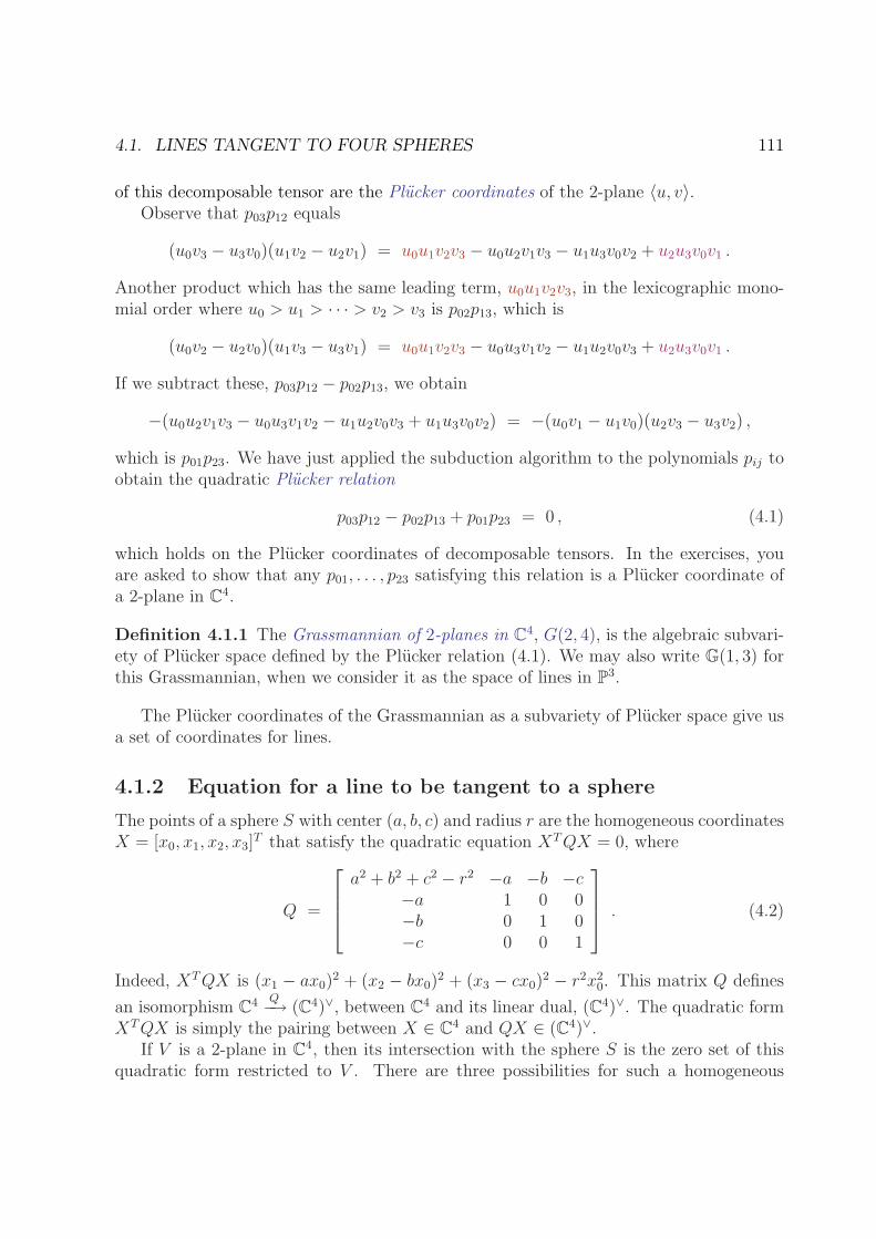
4.1. LINES TANGENT TO FOUR SPHERES 111
of this decomposable tensor are the Plucker coordinates of the 2-plane 〈u, v〉.Observe that p03p12 equals
(u0v3 − u3v0)(u1v2 − u2v1) = u0u1v2v3 − u0u2v1v3 − u1u3v0v2 + u2u3v0v1 .
Another product which has the same leading term, u0u1v2v3, in the lexicographic mono-mial order where u0 > u1 > · · · > v2 > v3 is p02p13, which is
(u0v2 − u2v0)(u1v3 − u3v1) = u0u1v2v3 − u0u3v1v2 − u1u2v0v3 + u2u3v0v1 .
If we subtract these, p03p12 − p02p13, we obtain
−(u0u2v1v3 − u0u3v1v2 − u1u2v0v3 + u1u3v0v2) = −(u0v1 − u1v0)(u2v3 − u3v2) ,
which is p01p23. We have just applied the subduction algorithm to the polynomials pij toobtain the quadratic Plucker relation
p03p12 − p02p13 + p01p23 = 0 , (4.1)
which holds on the Plucker coordinates of decomposable tensors. In the exercises, youare asked to show that any p01, . . . , p23 satisfying this relation is a Plucker coordinate ofa 2-plane in C4.
Definition 4.1.1 The Grassmannian of 2-planes in C4, G(2, 4), is the algebraic subvari-ety of Plucker space defined by the Plucker relation (4.1). We may also write G(1, 3) forthis Grassmannian, when we consider it as the space of lines in P3.
The Plucker coordinates of the Grassmannian as a subvariety of Plucker space give usa set of coordinates for lines.
4.1.2 Equation for a line to be tangent to a sphere
The points of a sphere S with center (a, b, c) and radius r are the homogeneous coordinatesX = [x0, x1, x2, x3]
T that satisfy the quadratic equation XTQX = 0, where
Q =
a2 + b2 + c2 − r2 −a −b −c−a 1 0 0−b 0 1 0−c 0 0 1
. (4.2)
Indeed, XTQX is (x1 − ax0)2 + (x2 − bx0)
2 + (x3 − cx0)2 − r2x2
0. This matrix Q defines
an isomorphism C4 Q−→ (C4)∨, between C4 and its linear dual, (C4)∨. The quadratic formXTQX is simply the pairing between X ∈ C4 and QX ∈ (C4)∨.
If V is a 2-plane in C4, then its intersection with the sphere S is the zero set of thisquadratic form restricted to V . There are three possibilities for such a homogeneous

112 CHAPTER 4. UNSTRUCTURED MATERIAL
quadratic form on V ≃ C2. If it is non-zero, then it factors. Either it has two distinctfactors, and thus the line corresponding to V meets the sphere in 2 distinct points, orelse it is the square of a linear form, and thus the line is tangent to the sphere. Thethird possibility is that it is zero, in which case, the line lies on the sphere (such a lineis necessarily imaginary) and is tangent to the sphere at every point of the line. Thethree cases are distinguished by the rank of the matrix representing the quadratic form(Exercise 3). In particular, the line is tangent to the sphere if and only if the determinantof this matrix vanishes.
We investigate its determinant. This restriction is defined by the composition of maps
V → C4 Q−−→ (C4)∨ ։ V ∨ , (4.3)
where the last map is the restriction of a linear form on C4 to V . The line represented by Vis tangent to S if and only if this quadratic form is degenerate, which means that the mapdoes not have full rank. To take the determinant of this map between two-dimensionalvector spaces, we apply the second exterior power ∧2 to the composition (4.3) and obtain
∧2V → ∧2C4 ∧2Q−−−→ ∧2(C4)∨ ։ ∧2V ∨ .
Since the image of ∧2V in ∧2C4 is spanned by the Plucker vector p of ∧2V and werestrict a linear form on ∧2C4 to ∧2V ∨ by evaluating it at p, we obtain the equation
pT ∧2Q p = 0 ,
for the line with Plucker coordinate p to be tangent to the sphere defined by the quadraticform Q.
If we express ∧2Q as a matrix with respect to the basis ei ∧ ej of ∧2C4, it will haverows and columns indexed by pairs ij with 0 ≤ i < j ≤ 3, where
(∧2Q)ij,kl := QikQjl −QilQjk = det
(
Qik Qil
Qjk Qjl
)
.
For our sphere (4.2), this is
∧2Q =
b2 + c2 − r2 −ab −ac b c 0−ab a2 + c2 − r2 −bc −a 0 c−ac −bc a2 + b2 − r2 0 −a −bb −a 0 1 0 0c 0 −a 0 1 00 c −b 0 0 1
010203121323
(4.4)
We remark that there is nothing special about spheres in this discussion.
Theorem 4.1.2 If q is any smooth quadric in P3 defined by a quadratic form Q, then aline with Plucker coordinate p is tangent to q if and only if pT ∧2Q p = 0, if and only if plies on the quadric in Plucker space defined by ∧2Q.

4.1. LINES TANGENT TO FOUR SPHERES 113
4.1.3 Solving the equations?
We may now formulate our problem of lines tangent to four spheres as the solutions toa system of equations. Namely, the set of lines tangent to four spheres have Pluckercoordinates in P5 which satisfy
1. The Plucker equation (4.1), and
2. Four quadratic equations of the form pT∧2Q p = 0, one for each sphere.
By Bezout’s theorem, we expect that there will be 25 solutions to these five quadraticequations on P5.
Let us investigate these equations. We will use the symbolic computation packageSingular [8] and display both annotated code and output in typewriter font. Outputlines begin with //, which are comment-line characters in Singular. First, we define ourground ring R to be Q[u, v, w, x, y, z] with the degree reverse lexicographic monomial orderwhere u > v > · · · > z. This is the coordinate ring of Plucker space, where we identifyp01 with u, p02 with v, p03 with w, and so on. We also declare the types of some variables.
ring R = 0, (u,v,w,x,y,z), dp;
matrix wQ[6][6];
matrix Pc[6][1] = u,v,w,x,y,z;
We give a procedure to compute ∧2Q (4.4),
proc Wedge_2_Sphere (poly r, a, b, c)
{
wQ = b^2+c^2-r^2 , -a*b , -a*c , b , c , 0,
-a*b , a^2+c^2-r^2 , -b*c , -a , 0 , c,
-a*c , -b*c , a^2+b^2-r^2 , 0 ,-a ,-b,
b , -a , 0 , 1 , 0 , 0,
c , 0 , -a , 0 , 1 , 0,
0 , c , -b , 0 , 0 , 1;
return(wQ);
}
and a procedure to compute the quadratic form pT∧2Q p.
proc makeEquation (poly r, a, b, c)
{
return((transpose(Pc)*WedgeTwoSphere(r,a,b,c)*Pc)[1][1]);
}
Now we create the ideal defining the lines tangent to four spheres with radii 1, 3/2, 2,and 2, and respective centers (0, 1, 1), (−1,−1, 0), (1,−1, 1), and (−2, 2, 0).

114 CHAPTER 4. UNSTRUCTURED MATERIAL
ideal I =
w*x-v*y+u*z,
makeEquation(1 , 0, 1, 1),
makeEquation(3/2 ,-1,-1, 0),
makeEquation(2 , 1,-1, 1),
makeEquation(2 ,-2, 2,0);
Lastly, we compute a Grobner basis for I and determine its dimension and degree.
I=std(I);
degree(I);
// dimension (proj.) = 1
// degree (proj.) = 4
This computation shows that the set of lines tangent to these four spheres has dimension1, so that there are infinitely many common tangents! This is not what we expected fromBezout’s Theorem and we must conclude that our equations are not sufficiently general.We will try to understand the special structure in our equations.
The key to this, as it turns out, is to use some classical facts about spheres. It is well-knkown that circles are exactly the conics in the plane P2 which contain the imaginarycircular points at infinity [0, 1,±i]. This is clear if we set x0 = 0 in the equation for acircle with center (a, b) and radius r,
(x1 − ax0)2 + (x2 − ax0)
2 = r2x20 .
For the same reason, spheres are the quadrics in P3 which contain the imaginary circularconic at infinity, which is defined by
x0 = 0 and x21 + x2
2 + x23 = 0 .
The lines at infinity have Plucker coordinates satisfying p01 = p02 = p03 = 0. For sucha point p, the equation pT∧2Qp, where Q is (4.4), becomes
p212 + p2
13 + p223 = 0 . (4.5)
This is the condition that the line at infinity is tangent to the spherical conic at infinity.Since the parameters r, a, b, c for the sphere do not appear in the equations p01 = p02 =p03 = 0 and (4.5), every line at infinity tangent to the spherical conic at infinity is tangentto every sphere.
In the language of enumerative geometry, this problem of lines tangent to four sphereshas excess intersection. That is, our equations for a line to be tangent to four spheres notonly define the lines we want (the tangent lines not at infinity), but also lines we did notintend, namely these lines tangent to the spherical conic at infinity.
If I is the ideal generated by our equations and J is the ideal of this excess component,then by Lemma 3.3.7, the saturation (I : J∞) is the ideal of V(I) \ V(J), which should

4.1. LINES TANGENT TO FOUR SPHERES 115
be the tangents that we seek. (We could also saturate by the ideal K = 〈p01, p02, p03〉of lines at infinity.) We return to our Singular computation, defining the ideal J andcomputing the quotient ideal (I : J). We do this instead of saturation, as saturation istypically computationally expensive.
ideal J = std(ideal(u,v,w,x^2+y^2+z^2));
I = std(quotient(I,J));
degree(I);
// dimension (proj.) = 1
// degree (proj.) = 2
While the degree of (I : J) is less than that of I, it is still 1-dimensional, so we take thequotient ideal again.
I = std(quotient(I,J));
degree(I);
// dimension (proj.) = 0
// degree (proj.) = 12
The dimension is now zero and we have removed the excess component from V(I).Since the dimension is 0 and the degree is 12, we expect that 12 is the answer to our
original question. That is, we expect that there will be 12 complex lines tangent to amyfour spheres in general position. In Exercise 6 we ask you to verify that there are indeed12 complex common tangent lines to the four spheres. Of these 12, six are real, and wedisplay them with the spheres below.
4.1.4 Twelve lines tanget to four general spheres
We remark that the computation of Section 4.1.3, while convincing, does not constitute aproof. We will give a rigorous proof here. Our basic idea to handle the excess component

116 CHAPTER 4. UNSTRUCTURED MATERIAL
is to simply define it away. Represent a line ℓ in R3 by a point p ∈ ℓ and a direction vectorv ∈ RP2.
p
vℓ
No such line can lie at infinity, so we are avoiding the excess component of lines at infinitytangent to the spherical conic at infinity.
Lemma 4.1.3 The set of direction vectors v ∈ RP2 of lines tangent to four spheres withaffinely independent centers consists of the common solutions to a cubic and a quarticequation on RP2. Each direction vector gives one common tangent.
Proof. For vectors x, y ∈ R3, let x · y be their ordinary Euclidean dot product and writex2 for x · x, which is ‖x‖2. Fix p to be the point of ℓ closest to the origin, so that
p · v = 0 . (4.6)
The distance from the line ℓ to a point c is ‖c− p‖ sin θ, where θ is the angle betweenv and the displacement vector from p to c.
cθ
c− p
‖c− p‖ sin θp
vℓ
This is the length of the cross product (c − p) × v, multiplied by the length ‖v‖ of thedirection vector v. If ℓ is tangent to the sphere with radius r centered at c ∈ R3 if itsdistance to c is r, and so we have ‖(c− p)× v‖ = r‖v‖. Squaring, we get
[(c− p)× v]2 = r2v2 . (4.7)
This formulation requires that v2 6= 0. A line with v2 = 0 has a complex direction vectorand it meets the spherical conic at infinity.
We assume that one sphere is centered at the origin and has radius r, while the otherthree have centers and radii (ci, ri) for i = 1, 2, 3. The condition for the line to be tangentto the sphere centered at the origin is
p2 = r2 . (4.8)

4.1. LINES TANGENT TO FOUR SPHERES 117
For the other spheres, we expand (4.7), use vector product identities, and the equa-tions (4.6) and (4.8) to obtain the vector equation
2v2
cT1cT2cT3
· p = −
(c1 · v)2
(c2 · v)2
(c3 · v)2
+ v2
c21 + r2 − r21
c22 + r2 − r22
c23 + r2 − r23
. (4.9)
Now suppose that the spheres have affinely independent centers. Then the matrix(c1, c2, c3)
T appearing in (4.9) is invertible. Assuming v2 6= 0, we may use (4.9) to write pas a quadratic function of v. Substituting this expression into equations (4.6) and (4.8),we obtain a cubic and a quartic equation for v ∈ RP2. The lemma now follows fromBezout’s Theorem. �
Bezout’s Theorem implies that there are at most 3 · 4 = 12 isolated solutions to theseequations, and over C exactly 12 if they are generic. The equations are however far fromgeneric as they involve only 13 parameters while the space of quartics has 14 parametersand the space of cubics has 9 parameters.
Example 4.1.4 Suppose that the spheres have equal radii, r, and have centers at thevertices of a regular tetrahedron with side length 2
√2,
(2, 2, 0)T , (2, 0, 2)T , (0, 2, 2)T , and (0, 0, 0)T .
In this symmetric case, the cubic factors into three linear factors. There are real commontangents only if
√2 ≤ r ≤ 3/2, and exactly 12 when the inequality is strict. If r =
√2, then
the spheres are pairwise tangent and there are three common tangents, one for each pairof non-intersecting edges of the tetrahedron. Each tangent has algebraic multiplicity 4.If r = 3/2, then there are six common tangents, each of multiplicity 2. The spheres meetpairwise in circles of radius 1/2 lying in the plane equidistant from their centers. Thisplane also contains the centers of the other two spheres, as well as one common tangentwhich is parallel to the edge between those centers.
Figure 4.1 shows the cubic (which consists of three lines supporting the edges of anequilateral triangle) and the quartic, in an affine piece of the set RP2 of direction vectors.The vertices of the triangle are the standard coordinate directions (1, 0, 0)T , (0, 1, 0)T , and(0, 0, 1)T . The singular cases, (i) when r =
√2 and (ii) when r = 3/2, are shown first,
and then (iii) when r = 1.425. The 12 points of intersection in this third case are visiblein the expanded view in (iii′). Each point of intersection gives a real tangent, so there are12 tangents to four spheres of equal radii 1.425 with centers at the vertices of the regulartetrahedron with edge length 2
√2.
One may also see this number 12 using group theory. The symmetry group of thetetrahedron, which is the group of permutations of the spheres, acts transitively on theircommon tangents and the isotropy group of any tangent has order 2. To see this, orienta common tangent and suppose that it meets the spheres a, b, c, d in order. Then thepermutation (a, d)(b, c) fixes that tangent but reverses its orientation, and the identity isthe only other permutation fixing that tangent.

118 CHAPTER 4. UNSTRUCTURED MATERIAL
(i) (ii)
(iii) (iii′)
Figure 4.1: The cubic and quartic for symmetric configurations.
This example shows that the bound of 12 common tangents from Lemma 4.1.3 is infact attained.
Theorem 4.1.5 There are at most 12 common real tangent lines to four spheres whosecenters are not coplanar, and there exist spheres with 12 common real tangents.
Example 4.1.6 We give an example when the radii are distinct, namely 1.4, 1.42, 1.45,and 1.474. Figure 4.2 shows the quartic and cubic and the configuration of 4 spheres andtheir 12 common tangents.
Now suppose that the centers are coplanar. A continuity argument shows that fourgeneral such spheres will have 12 complex common tangents (or infinitely many, but thispossibility is precluded by the following example). Three spheres of radius 4/5 centeredat the vertices of an equilateral triangle with side length
√3 and one of radius 1/3 at
the triangle’s center have 12 common real tangents. We display this configuration inFigure 4.3. This configuration of spheres has symmetry group Z2 ×D3, which has order12 and acts faithfully and transitively on the common tangents.
In the symmetric configuration of Example 4.1.4 having 12 common tangents, everypair of spheres meet. It is however not necessary for the spheres to meet pairwise whenthere are 12 common tangents. In fact, in both Figures 4.2 and 4.3 not all pairs of spheres

4.1. LINES TANGENT TO FOUR SPHERES 119
Figure 4.2: Spheres with 12 common tangents.
meet. However, the union of the spheres is connected. This turns out to be unnecessary.In the tetrahedral configuration, if one sphere has radius 1.38 and the other three haveequal radii of 1.44, then the first sphere does not meet the others, but there are still 12tangents.
More interestingly, it is possible to have 12 common real tangents to four disjointspheres. Figure 4.4 displays such a configuration. The three large spheres have radius4/5 and are centered at the vertices of an equilateral triangle of side length
√3, while the
smaller sphere has radius 1/4 and is centered on the axis of symmetry of the triangle, butat a distance of 35/100 from the plane of the triangle.
Exercises
1. Show that if u ∧ v and x ∧ y are two decomposable tensors representing the samepoint in P(∧2C4), then they come from the same 2-plane in C4. That is, show that〈u, v〉 = 〈x, y〉.
2. Show that if [p01, . . . , p23] are the homogeneous coordinates of a point of P(∧2C4)that satisfies the Plucker relation, then this is the Plucker coordinate of a 2-planein C4.
3. Let Q be a symmetric 2 × 2 matrix. Show that the quadratic form XTQX hasdistinct factors if and only if Q is invertible. If Q has rank 1, then show that XTQXis the square of a linear form, and that XTQX is the zero polynomial only when Qhas rank zero.
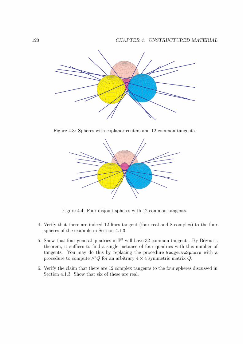
120 CHAPTER 4. UNSTRUCTURED MATERIAL
Figure 4.3: Spheres with coplanar centers and 12 common tangents.
Figure 4.4: Four disjoint spheres with 12 common tangents.
4. Verify that there are indeed 12 lines tangent (four real and 8 complex) to the fourspheres of the example in Section 4.1.3.
5. Show that four general quadrics in P3 will have 32 common tangents. By Bezout’stheorem, it suffices to find a single instance of four quadrics with this number oftangents. You may do this by replacing the procedure WedgeTwoSphere with aprocedure to compute ∧2Q for an arbitrary 4× 4 symmetric matrix Q.
6. Verify the claim that there are 12 complex tangents to the four spheres discussed inSection 4.1.3. Show that six of these are real.

Appendix A
Appendix
A.1 Algebra
Algebra is the foundation of algebraic geometry; here we collect some of the basic algebraon which we rely. We develop some algebraic background that is needed in the text. Thismay not be an adequate substitute for a course in abstract algebra. Proofs can be foundin give some useful texts.
A.1.1 Fields and Rings
We are all familiar with the real numbers, R, with the rational numbers Q, and withthe complex numbers C. These are the most common examples of fields, which are thebasic building blocks of both the algebra and the geometry that we study. Formallyand briefly, a field is a set F equipped with operations of addition and multiplicationand distinguished elements 0 and 1 (the additive and multiplicative identities). Everynumber a ∈ F has an additive inverse −a and every non-zero number a ∈ F× := F− {0}has a multiplicative inverse a−1 =: 1
a. Addition and multiplication are commutative and
associative and multiplication distributes over addition, a(b + c) = ab + ac. To avoidtriviality, we require that 0 6= 1.
The set of integers Z is not a field as 12
is not an integer. While we will mostly beworking over Q, R, and C, at times we will need to discuss other fields. Most of whatwe do in algebraic geometry makes sense over any field, including the finite fields. Inparticular, linear algebra (except numerical linear algebra) works over any field.
Linear algebra concerns itself with vector spaces. A vector space V over a field F
comes equipped with an operation of addition—we may add vectors and an operation ofmultiplication—we may multiply a vector by an element of the field. A linear combinationof vectors v1, . . . , vn ∈ V is any vector of the form
a1v1 + a2v2 + · · ·+ anvn ,
where a1, . . . , an ∈ F. A collection S of vectors spans V if every vector in V is a linear
121

122 APPENDIX A. APPENDIX
combination of vectors from S. A collection S of vectors is linearly independent if zerois not nontrivial linear combination of vectors from S. A basis S of V is a linearlyindependent spanning set. When a vector space V has a finite basis, every other basis hasthe same number of elements, and this common number is called the dimension of V .
A ring is the next most complicated object we encounter. A ring R comes equippedwith an addition and a multiplication which satisfy almost all the properties of a field,except that we do not necessarily have multiplicative inverses. While the integers Z donot form a field, they do form a ring. An ideal I of a ring R is a subset which is closedunder addition and under multiplication by elements of R. Every ring has two trivialideals, the zero ideal {0} and the unit ideal consisting of R itself. Given a set S ⊂ R ofelements, the smallest ideal containing S, also called the ideal generated by S, is
〈S〉 := {r1s1 + r2s2 + · · ·+ rmsm | r1, . . . , rm ∈ R and s1, . . . , sm ∈ S} .
A primary use of ideals in algebra is through the construction of quotient rings. LetI ⊂ R be an ideal. Formally, the quotient ring R/I is the collection of all sets of the form
[r] := r + I = {r + s | s ∈ I} ,
as r ranges over R. Addition and multiplication of these sets are defined in the usual way
[r] + [s] = {r′ + s′ | r′ ∈ [r] and s′ ∈ [s]} != [r + s], and
[r] · [s] = {r′ · s′ | r′ ∈ [r] and s′ ∈ [s]} != [rs] .
The last equality (!=) in each line is meant to be surprising, it is a theorem and due to
I being an ideal. Thus addition and multiplication on R/I are inherited from R. Withthese definitions (and also −[r] = [−r], 0 := [0], and 1 := [1]), the set R/I becomes aring.
We say ‘R-mod-I’ for R/I because the arithmetic in R/I is just the arithmetic in R,but considered modulo the ideal I, as [r] = [s] in R/I if and only if r − s ∈ I.
Ideals also arise naturally as kernels of homomorphisms. A homomorphism ϕ : R→ Sfrom the ring R to the ring S is a function that preserves the ring structure. Thus forr, s ∈ R, ϕ(r + s) = ϕ(r) + ϕ(s) and ϕ(rs) = ϕ(r)ϕ(s). We also require that ϕ(1) = 1.The kernel of a homomorphism ϕ : R→ S,
kerϕ := {r ∈ R | ϕ(r) = 0}
is an ideal: If r, s ∈ kerϕ and t ∈ R, then
ϕ(r + s) = ϕ(r) + ϕ(s) = 0 = tϕ(r) = ϕ(tr) .
Homomorphisms are deeply intertwined with ideals. If I is an ideal of a ring R, thenthe association r 7→ [r] defines a homomorphism ϕ : R → R/I whose kernel is I. Dually,given a homomorphism ϕ : R→ S, the image of R in S is identified with R/ kerϕ. More

A.1. ALGEBRA 123
generally, if ϕ : R→ S is a homomorphism and I ⊂ R is an ideal with I ⊂ kerϕ (that is,ϕ(I) = 0), then ϕ induces a homomorphism ϕ : R/I → S.
Properties of ideals induce natural properties in the associated quotient rings. Anelement r of a ring R is nilpotent if r 6= 0, but some power of r vanishes. A ring R isreduced if it has no nilpotent elements, that is, whenever r ∈ R and n is a natural numberwith rn = 0, then we must have r = 0. An ideal radical if whenever r ∈ R and n is anatural number with rn ∈ I, then we must have r ∈ I. It follows that a quotient ring R/Iis reduced if and only if I is radical.
A ring R is a domain if whenever we have r · s = 0 with r 6= 0, then we must haves = 0. An ideal is prime if whenever r · s ∈ I with r 6∈ I, then we must have s ∈ I. Itfollows that a quotient ring R/I is a domain if and only if I is prime.
A ring R with no nontrivial ideals must be a field. Indeed, if 0 6= r ∈ R, then the idealrR of R generated by r is not the zero ideal, and so it must equal R. But then 1 = rsfor some s ∈ R, and so r is invertible. Conversely, if R is a field and 0 6= r ∈ R, then1 = r · r−1 ∈ rR, so the only ideals of R are {0} and R. An ideal m of R is maximalif m ( R, but there is no ideal I strictly contained between m and R; if m ⊂ I ⊂ Rand I 6= R, then I = m. It follows that a quotient ring R/I is a field if and only if I ismaximal.
Lastly, we remark that any ideal I of R with I 6= R is contained in some maximalideal. Suppose not. Then we may find an infinite chain of ideals
I =: I0 ( I1 ( I2 ( · · ·
where each is proper so that 1 lies in none of them. Set J :=⋃
n In. Then we claim thatthe union I :=
⋃
n In of these ideals is an ideal. Indeed, if r, s ∈ I then there are indicesi, j with r ∈ Ii and s ∈ Ij. Since Ii, Ij ⊂ Imax(i,j), we have r + s ∈ Imax(i,j) ⊂ J . If t ∈ R,then tr ∈ Ii ⊂ J
A.1.2 Fields and polynomials
Our basic algebraic objects are polynomials. A univariate polynomial p is an expressionof the form
p = p(x) := a0 + a1x+ a2x2 + · · ·+ amx
m , (A.1)
where m is a nonnegative integer and the coefficients a0, a1, . . . , am lie in F. Write F[x] forthe set of all polynomials in the variable x with coefficients in F. We may add, subtract,and multiply polynomials and F[x] is a ring.
While a polynomial p may be regarded as a formal expression (A.1), evaluation of apolynomial defines a function p : F → F: The value of the function p at a point a ∈ F issimply p(a). When F is infinite, the polynomial and the function determine each other,but this is not the case when F is finite.
Our study requires polynomials with more than one variable. We first define a mono-mial.

124 APPENDIX A. APPENDIX
Definition A.1.1 A monomial in the variables x1, . . . , xn is a product of the form
xα1
1 xα2
2 · · ·xαn
n ,
where the exponents α1, . . . , αn are nonnegative integers. For notational convenience, setα := (α1, . . . , αn) ∈ Nn† and write xα for the expression xα1
1 · · ·xαnn . The (total) degree of
the monomial xα is |α| := α1 + · · ·+ αn.
A polynomial f = f(x1, . . . , xn) in the variables x1, . . . , xn is a linear combination ofmonomials, that is, a finite sum of the form
f =∑
α∈Nn
aαxα ,
where each coefficient aα lies in F and all but finitely many of the coefficients vanish. Theproduct aαx
α of an element aα of F and a monomial xα is called a term. The supportA ⊂ Nn of a polynomial f is the set of all exponent vectors that appear in f with anonzero coefficient. We will say that f has support A when we mean that the support off is a subset of A.
After 0 and 1 (the additive and multiplicative identities), the most distinguished in-tegers are the prime numbers, those p > 1 whose only divisors are 1 and themselves.These are the numbers 2, 3, 5, 7, 11, 13, 17, 19, 23, . . . Every integer n > 1 has a uniquefactorization into prime numbers
n = pα1
1 pα2
1 · · · pαn
n ,
where p1 < · · · < pn are distinct primes, and α1, . . . , αn are (strictly) positive integers.For example, 999 = 33 · 37. Polynomials also have unique factorization.
Definition A.1.2 A nonconstant polynomial f ∈ F[x1, . . . , xn] is irreducible if wheneverwe have f = gh with g, h polynomials, then either g or h is a constant. That is, f has nonontrivial factors.
Theorem A.1.3 Every polynomial f ∈ F[x1, . . . , xn] is a product of irreducible polyno-mials
f = p1 · p2 · · · pm ,where the polynomials p1, . . . , pm are irreducible and nonconstant. Moreover, this factor-ization is essentially unique. That is, if
f = q1 · q2 · · · qs ,
is another such factorization, then m = s, and after permuting the order of the factors,each polynomial qi is a scalar multiple of the corresponding polynomial pi.
†Where have we defined N?

A.1. ALGEBRA 125
A.1.3 Polynomials in one variable
While rings of polynomials have many properties in common with the integers, the relationis the closest for univariate polynomials. The degree, deg(f) of a univariate polynomialf is the largest degree of a monomial appearing in f . If this monomial has coefficient 1,then the polynomial is monic. This allows us to remove the ambiguity in the uniquenessof factorizations in Theorem A.1.3. A polynomial f(x) ∈ F[x] has a unique factorizationof the form
f = fm · pα1
1 · pα2
2 · · · pαs
s ,
where fm ∈ F× is the leading coefficient of f , the polynomials p1, . . . , ps are monic andirreducible, and the exponents αi are positive integers.
Definition A.1.4 A greatest common divisor of two polynomials f, g ∈ F[x] (or gcd(f, g))is a polynomial h such that h divides each of f and g, and if there is another polynomialk which divides both f and g, then k divides h.
Any two polynomials f and g have a monic greatest common divisor which is theproduct of the common monic irreducible factors of f and g, each raised to the highestpower that divides both f and g. Finding greatest common divisor would seem challengingas factoring polynomials is not an easy task. There is, however, a very fast and efficientalgorithm for computing the greatest common divisor of two polynomials.
Suppose that we have polynomials f and g in F[x] with deg(g) ≥ deg(f),
f = f0 + f1x+ f2x2 + · · ·+ fmx
m
g = g0 + g1x+ g2x2 + · · ·+ gmx
m + · · ·+ gnxn ,
where fm and gn are nonzero. Then the polynomial
S(f, g) := g − gnfmxn−m · f
has degree strictly less than n = deg(g). This simple operation of reducing f by thepolynomial g forms the basis of the Division Algorithm and the Euclidean Algorithm forcomputing the greatest common divisor of two polynomials.
We describe the Division Algorithm in pseudocode, which is a common way to explainalgorithms without reference to a specific programming language.
Algorithm A.1.5 [Division Algorithm]Input: Polynomials f, g ∈ F[x].Output: Polynomials q, r ∈ F[x] with g = qf + r and deg(r) < deg(f).Set r := g and q := 0.(1) If deg(r) < deg(f), then exit.(2) Otherwise, reduce r by f to get the expression
r =rnfmxn−m · f + S(f, r) ,

126 APPENDIX A. APPENDIX
where n = deg(r) and m = deg(f). Set q := q + rnfmxn−m and r := S(f, r), and return to
step (1).
To see that this algorithm does produce the desired expression g = qf + r with thedegree of r less than the degree of f , note first that whenever we are at step (1), we willalways have g = qf + r. Also, every time step (2) is executed, the degree of r must drop,and so after at most deg(g) − deg(f) + 1 steps, the algorithm will halt with the correctanswer.
The Euclidean Algorithm computes the greatest common divisor of two polynomials fand g.
Algorithm A.1.6 [Euclidean Algorithm]Input: Polynomials f, g ∈ F[x].Output: The greatest common divisor h of f and g.(1) Call the Division Algorithm to write g = qf + r where deg(r) < deg(f).(2) If r = 0 then set h := f and exit.
Otherwise, set g := f and f := r and return to step (1).
To see that the Euclidean algorithm performs as claimed, first note that if g = qf + rwith r = 0, then f = gcd(f, g). If r 6= 0, then gcd(f, g) = gcd(f, r). Thus the greatestcommon divisor h of f and g is always the same whenever step (1) is executed. Since thedegree of r must drop upon each iteration, r will eventually become 0, which shows thatthe algorithm will halt and return h.†
An ideal is principal if it has the form
〈f〉 = {h · f | h ∈ F[x]} ,
for some f ∈ F[x]. We say that f generates 〈f〉. Since 〈f〉 = 〈αf〉 for any α ∈ F, theprincipal ideal has a unique monic generator.
Theorem A.1.7 Every ideal I of F[x] is principal.
Proof. Suppose that I is a nonzero ideal of F[x], and let f be a nonzero polynomial ofminimal degree in I. If g ∈ I, then we may apply the Division Algorithm and obtainpolynomials q, r ∈ F[x] with
g = qf + r with deg(r) < deg(f) .
Since r = g− qf , we have r ∈ I, and since deg(r) < deg(f), but f had minimal degree inI, we conclude that f divides g, and thus I = 〈f〉. �
†This is poorly written!

A.2. TOPOLOGY 127
The ideal generated by univariate polynomials f1, . . . , fs is the principal ideal 〈p〉,where p is the greatest common divisor of f1, . . . , fs.
For univariate polynomials p the quotient ring F[x]/〈p〉 has a concrete interpretation.Given f ∈ F[x], we may call the Division Algorithm to obtain polynomials q, r with
f = q · p+ r, where deg(r) < deg(q) .
Then [f ] = f + 〈p〉 = r + 〈p〉 = [r] and in fact r is the unique polynomial of minimaldegree in the coset f + 〈p〉. We call this the normal form of f in F[x]/〈p〉.
Since, if deg(r), deg(s) < deg(p), we cannot have r− s ∈ 〈p〉 unless r = s, we see thatthe monomials 1, x, x2, . . . , xdeg(p)−1 form a basis for the F-vector space F[x]/〈p〉. Thisdescribes the additive structure on F[x]/〈p〉.
To describe its multiplicative structure, we only need to show how to write a productof monomials xa · xb with a, b < deg(p) in this basis. Suppose that p is monic withdeg(p) = n and write p(x) = xn − q(x), where q has degree strictly less than p. Sincexa · xb = (xa · x) · xb−1, we may assume that b = 1. When a < n, we have xa · x1 = xa+1.When a = n− 1, then xn−1 · x1 = xn = q(x),
• Relate algebraic properties of p(x) to properties of R, for example, zero divisors anddomain.
• Prove that a field is a ring with only trivial ideals.
Prove I ⊂ J ⊂ R are ideals, then J/I is an ideal of R/I, and deduce that R =F[x]/p(x) is a field only if p(x) is irreducible.
Example Q[x]/(x2 − 2) and explore Q(√
2).
Example R[x]/(x2 + 1) and show how it is isomorphic to C.
Work up to algebraically closed fields, the fundamental theorem of algebra (bothover C and over R).
Explain that an algebraically closed field has no algebraic extensions (hence thename).
• Define the maximal ideal ma for a ∈ An.
Theorem A.1.8 The maximal ideals of C[x1, . . . , xn] all have the form ma for somea ∈ An.
A.2 Topology
Collect some topological statements here. Definition of topology, Closed/open duality, dense,nowhere dense... Describe the usual topology.
Recall that a function f : X → Y is continuous if and only if whenever Z ⊂ Y is aclosed set f−1(Z) ⊂ X is also closed.

128 APPENDIX A. APPENDIX

Bibliography
[1] Etienne Bezout, Theorie generale des equations algebriques, Ph.-D. Pierres, 1779.
[2] , General theory of algebraic equations, Princeton University Press, 2006,Translated from French original by Eric Feron.
[3] B. Buchberger, Ein algorithmisches Kriterium fur die Losbarkeit eines algebraischenGleichungssystems, Aequationes Math. 4 (1970), 374–383.
[4] Bruno Buchberger, An algorithm for finding the basis elements of the residue classring of a zero dimensional polynomial ideal, J. Symbolic Comput. 41 (2006), no. 3-4,475–511, Translated from the 1965 German original by Michael P. Abramson.
[5] David Cox, John Little, and Donal O’Shea, Ideals, varieties, and algorithms, thirded., Undergraduate Texts in Mathematics, Springer, New York, 2007, An introduc-tion to computational algebraic geometry and commutative algebra.
[6] J.-C. Faugere, FGb, See http://fgbrs.lip6.fr/jcf/Software/FGb/index.html.
[7] J. C. Faugere, P. Gianni, D. Lazard, and T. Mora, Efficient computation of zero-dimensional Grobner bases by change of ordering, J. Symbolic Comput. 16 (1993),no. 4, 329–344.
[8] G.-M. Greuel, G. Pfister, and H. Schonemann, Singular 3.0, A Computer AlgebraSystem for Polynomial Computations, Centre for Computer Algebra, University ofKaiserslautern, 2005, http://www.singular.uni-kl.de.
[9] Raymond Hemmecke and Peter Malkin, Computing generating sets of lattice ideals,math.CO/0508359.
[10] H. Hironaka, Resolution of singularities of an algebraic variety over a field of char-acteristic zero, Ann. Math. 79 (1964), 109–326.
[11] Serkan Hosten and Bernd Sturmfels, GRIN: an implementation of Grobner bases forinteger programming, Integer programming and combinatorial optimization (Copen-hagen, 1995), Lecture Notes in Comput. Sci., vol. 920, Springer, Berlin, 1995, pp. 267–276.
129
130 BIBLIOGRAPHY
[12] T. Y. Li, Tim Sauer, and J. A. Yorke, The cheater’s homotopy: an efficient procedurefor solving systems of polynomial equations, SIAM J. Numer. Anal. 26 (1989), no. 5,1241–1251.
[13] F.S. Macaulay, Some properties of enumeration in the theory of modular systems,Proc. London Math. Soc. 26 (1927), 531–555.
[14] Andrew J. Sommese and Charles W. Wampler, II, The numerical solution of systemsof polynomials, World Scientific Publishing Co. Pte. Ltd., Hackensack, NJ, 2005,Arising in engineering and science.