Discovering Interacting Artifacts from ERP Systems(Extended Version)

Xixi Lu1, Marijn Nagelkerke2, Dennis van de Wiel2, and Dirk Fahland1

1 Eindhoven University of Technology, The Netherlands2 KPMG IT Advisory N.V., Eindhoven, The Netherlands.

(x.lu,d.fahland)@tue.nl(Nagelkerke.marijn,vandewiel.dennis)@kpmg.nl

Abstract. The omnipresence of using Enterprise Resource Planning (ERP) sys-tems to support business processes has enabled recording a great amount of (re-lational) data which contains information about the behaviors of these processes.Various process mining techniques have been proposed to analyze recorded in-formation about process executions. However, classic process mining techniquesgenerally require a linear event log as input and not a multi-dimensional rela-tional database used by ERP systems. Much research has been conducted intoconverting a relational data source into an event log. Most conversion approachesfound in literature usually assume a clear notion of a case and a unique case iden-tifier in an isolated process. This assumption does not hold in ERP systems whereprocesses comprise the life-cycles of various interrelated data objects, instead ofa single process. In this paper, a new semi-automatic approach is presented todiscover from the plain database of an ERP system the various objects supportingthe system. More precisely, we identify an artifact-centric process model describ-ing the system’s objects, their life-cycles, and detailed information about how thevarious objects synchronize along their life-cycles, called interactions. In addi-tion, our artifact-centric approach helps to eliminate ambiguous dependencies indiscovered models caused by the data divergence and convergence problems andto identify the exact “abnormal flows”. The presented approach is implementedand evaluated on two processes of ERP systems through case studies.

Keywords: Process Discovery, Artifact-Centric Processes, Outlier Detection, Rela-tional Data, Log Conversion, ERP Systems

1 Introduction

Information systems (IS) not only store and process data in an organization but alsorecord event data about how and when information changed. This “historical eventdata” is often used to analyze, for instance, whether information processing in the pastconformed to the processes in the organization or to compliance regulations. For exam-ple, has each order by a gold customer been delivered with priority shipping, or haveall delivery documents been created before creating the invoice? The manual analysisof historic event data is time consuming and error-prone as often hundreds of thousandsof records need to be checked.

Documents Changes

Change id Date changed Reference id Table name Change type Old Value New Value

1 17-5-2020 S1 SD Price updated 100 80

2 19-5-2020 S1 SD Delivery block released X -

3 19-5-2020 S1 SD Billing block released X -

4 10-6-2020 B1 BD Invoice date updated 20-6-2020 21-6-2020

Billing documents (BD)

BD id Date created Document type Clearing date

B1 20-5-2020 Invoice 31-5-2020

B2 24-5-2020 Invoice 5-6-2020

Delivery documents (DD)

DD id Date created Reference SD id Reference BD Document type Picking date

D1 18-5-2020 S1 B1 Delivery 31-5-2020

D2 22-5-2020 S1 B2 Delivery 5-6-2020

D3 25-5-2020 S2 B2 Delivery 5-6-2020

D4 12-6-2020 S3 null Return Delivery NULL

Sales documents (SD)

SD id Date created Reference id Document type Value Last change

S1 16-5-2020 null Sales Order 100 10-6-2020

S2 17-5-2020 null Sales Order 200 31-5-2020

S3 10-6-2020 S1 Return Order 10 NULL

F1

F2

F4 F3

Parent

table

Child

table

Fig. 1: The tables of the simplified OTC example

Process mining [1] offers automated techniques for this task. The most prominenttechnique is to discover from historical event data a graphical process model describ-ing all historic behaviors; the discovered model can be visually explored to identify themain flows and the unusual flows of the process. Process analyst and domain expert canthen for instance identify the historic events that correspond to unusual flows, investi-gate circumstances and possible causes for this behavior, and devise concrete measuresto improve the process [2]. The success of the analysis often depends on whether un-usual behavior is easy to distinguish visually from normal behavior. Prerequisite to thisanalysis is a process event log that describes how all information changes occurred fromthe perspective of a particular process; its underlying assumption is that each event canunambiguously be mapped to a particular case of the process.

1.1 Problem Description

In the more general case, information access is not tied to a particular case of a process;rather the same information can be accessed and changed from various processes andapplications. A typical example are Enterprise Resource Planning (ERP) systems whichorganize all information in documents related to each other through one-to-many andmany-to-many relations; information changes occur in transactions and the completionof a transaction is logged as an event also called transactional data. All data relevantfor the analysis is stored in a relational database.

Figure 1 shows a simplified example of the transactional data of an Order to Cash(OTC) process supported by SAP systems; Fig. 2 visualizes the events stored in thesetables related to the creation of documents. There are two sales orders S1 and S2; cre-ation of S1 is followed by creation of a delivery document D1, an invoice B1, anotherdelivery document D2, and another invoice B2 which also contains billing informationabout S2. Creation of S2 is also followed by creation of another delivery document D3.Further, there is a return order S3 related to S1 with its own return delivery documentD4. The many-to-many relations between documents surface in the transactional data:a sales document can be related to multiple billing documents (S1 is related to B1 andB2) and a billing document can be related to multiple sales document (B2 is related toS1 and S2). This behavior already contains an unusual flow: two times delivery doc-

PAGE 34

15-5 20-5 25-5 9-6

S1 created on 16-5

D1 created on 18-5

D2 created on 22-5

B1 created on 20-5

B2 created on 24-5

S2 created 17-5 D3 created 25-5

B2 created 24-5

S3 created on 10-6

D4 created on 22-5

Creation of documents related to S1

Creation of documents related to S2

Timeline

Fig. 2: A time-line regarding the creation of documents of the OTC example.

uments were created before the billing document (main flow), but once the order wasreversed (B2 before D3).

The main research problem addressed in this paper is to provide (semi-)automatedtechniques to

(1) discover from the relational transactional data of an ERP system an accurate graph-ical model describing all transactions and their order, and

(2) identify main flows and unusual flows and highlight the latter ones.

Classical process mining techniques cannot be applied directly. Many previous studieshave shown that an attempt to cast transactional data over objects with many-to-manyrelations into a single process event log and discovering a single process model describ-ing all transactional data is bound to fail. It leads to false dependencies between eventsand duplicate events which obscures the main flow and hinder the detection of unusualflows [3] [4] [5] [6] [7].

1.2 Proposed Solution

We propose to approach the problem under the “conceptual lens” of artifact-centricmodels [8, 9]. An artifact is a data object over an information model; each artifact in-stances exposes services that allow changing its informational contents; a life-cyclemodel governs when which service of the artifact can be invoked; the invocation of aservice in one artifact may trigger the invocation of another service in another artifact.Information models of different artifacts can be in one-to-many and many-to-many rela-tions, which allows to describe behavior over complex data in terms of multiple objectsinteracting via service invocations. We apply the artifact-centric view to our problemas follows: each document of an ERP system can be seen as an artifact; transactionson the document are service calls on the artifacts; behavioral dependencies betweentransactions of documents can be seen as life-cycle behavior and dependencies of ser-vice calls. With these concepts, the transactional data of Fig. 1 can be described as the

Fig. 3: Artifact-centric model of the behavior in Fig. 1

artifact-centric model of Fig. 3. The model visualizes the order in which objects arecreated and also highlights the unusual flow of invoice B2 being created before deliveryD2.

The problem of discovering an artifact-centric process model from relational ERPdata decomposes into two sub-problems:

(1) Given a relational data source, identify a set of artifact types on the database level,extract for each artifact type an event log and discover its life-cycle.

(2) Given a relational data source, a set of artifact types and their corresponding setof logs, identify interactions between the artifact types, between their instances,between their event types and between their events. As a result, obtain a completeartifact-centric process model.

Figure 4 shows the overview of our approach. The flow of our approach that ad-dresses the first problem of discovering artifact’s life-cycles is shown by the filled arcs,whereas the second problem of discovering interactions between artifacts is addressedby the flow shown by the dashed arcs. In a nutshell, (1.1) we use the data schema todiscover artifact schemas from which (1.2) we discover artifact types; each artifact typedescribes the information model of one artifact in terms of the attributes found in thedata source. Each record in the data source defines an artifact instance. For each artifacttype, (1.3) we extract its instances and all related events; all events related to one arti-fact instance are grouped together into a case of this instance and ordered by time. Thecase describes how the artifact instance evolved over time. All cases together yield theevent log of the artifact type. (1.4) We feed the event log of an artifact type to existingprocess discovery algorithms to obtain the life-cycle model of the artifact type. In par-allel, (2.1) we use the foreign key relations in the data schema to discover interactionsbetween artifact types and instances. (2.2) This information about interactions betweenartifact instances is also added to the respective cases in the extracted event logs. (2.3)We then propose two different techniques to derive from the interactions between casesinteractions between the events of the different cases. (2.4) Interactions between eventsare then generalized to interactions between life-cycle models.

We implemented our approach and conducted two case studies. In both case studiesthe discovered process models were assessed as accurate graphical representations of

the source data; insights about unusual flows could be obtained significantly faster thanwith existing best practices. Thereby, we also learned that the steps of (1.1-1.2) of iden-tifying artifact types and steps (2.1-2.4) are tightly related due to relations in the originalrelational data source. By choosing whether a relation is contained inside one artifacttype or between two artifact types, one also chooses whether there is an interactionbetween artifacts or not. In this paper, we will show that by moving all one-to-manyand many-to-many relations between artifact types in (1.1-1.2), the life-cycle modelsdiscovered in (1.4) have higher quality and the interactions discovered in (2.1-2.4) aremeaningful to business users.

The remainder of this paper is structured as follows. In Section 2, we provide a de-tailed problem analysis using a running example, showing the limitations of classicallog conversion approaches and motivating the use of an artifact-centric approach in-stead. Section 3 discusses related work. Section 4 illustrates our extended approach toidentify artifacts and their life-cycles from a given relational data source. In Section 5,we discuss interactions between artifacts on different levels and show how to identifythese interactions to obtain a complete artifact-centric model. The methodology used toconduct artifact-centric process analysis is presented in Section 6. We implemented ourtechnique and report on two case studies in Section 7. Section 8 concludes the paper.

2 Problem Analysis

In this section, we first introduce a running example that is used throughout the paper todemonstrate the concepts used in this paper and our approach. Using the running exam-ple, we then discuss why classical log conversions and process discovery techniques failto analyze ERP data sets. Then we introduce the artifact-centric approach and show thatit is better suited to describe ERP data sets allowing for a variety of results dependingon user choices.

2.1 Running Example

To illustrate the problem of process discovery from ERP data, we consider a simplifiedvariant of the Order to Cash process supported by SAP systems and use this as ourrunning example throughout the paper. In short, the OTC process starts with customersplacing orders. Then, the organization fulfills the orders by delivering the goods andsending invoices to bill the cost and receive payments from customers. Organizationsuse an ERP system to store documents of sales orders, deliveries, invoices and paymentsthat are related to the OTC process in tables similar to those shown in Figure 1. Webriefly explain the process executions that have led to the data in Figure 1, focusingonly on the creation of documents for the sake of brevity. First, a customer placed asales order S1, which is created in the system on May 16th. Then a partial delivery D1is done on May 18th, and the related invoice B1 is created two days later. On May 22th,another part of the sales order S1 is delivered according to the delivery document D2which is invoiced with document B2 on May 24th. On May 17th, the same customerplaces another sales order S2, which is also invoiced within the same billing documentB2. However, the delivery D3 related to the sales order S2 is executed after the billing

Artifact types

Database schema

Artifact schemas

Event logs

Life-cycles

Artifact-centric process model

Data Source

Import data schema

Use XTract

1.1 Discover Artifact Schemas

(Sect. 4.3)

1.2 Discover Artifacts

(Sect. 4.4)

1.3 Extract Logs (Sect. 4.5)

1.4 DiscoverLife-cycle (Sect. 4.7)

2.1 Discover artifact type level

interactions(Sect. 5.2)

2.2 Extract artifact instance level interactions

(Sect. 5.3)

2.3 Discover event type leveland event level

interactions(Sect. 5.4)

Refine or select by users

Refine or select by users

Case 1Case 2

…Case n

Case 1Case 2

…Case n

Case 1Case 2

…Case n

2.4 Discover Artifact-centric

Model (Sect. 5.5)

Discovering artifactsDiscovering interactions

Fig. 4: An overview of our approach.

document B2 on May 25th. Days later, a return order S3 is placed for the sales orderS1 and return delivery D4 is executed. A time-line of the events related to the creationsis shown in Figure 2, in which a distinction is made between the creation of documentsthat is related to the sales order S1 (above the line in Figure 2) or to S2 (below the linein Figure 2).

The data related to these executions are stored in four tables Sales Documents(SD),Delivery Documents(DD), Billing Documents(BD), and Document Changes(DC) shownin Figure 1. The table SD contains the two sales order documents S1 and S2 and thereturn order document S3. The foreign key F1 relates the sales documents to each other.The DD contains the three delivery documents D1, D2 and D3 and the return deliverydocument D4. The delivery and return delivery documents are related to the sales doc-uments via foreign key F2. The two invoices B1 and B2 are stored in the table BD haverelations with the delivery documents via foreign key F3. Any changes related to thedocuments are stored in the table Document Changes.

2.2 Classical Log Conversion and Process Discovery

Process mining is a set of techniques to “discover, monitor and improve real processes(i.e., not assumed processes) by extracting knowledge from event logs” [10]. In thispaper, we focus on process discovery, which aims to discover a process model from agiven event log.

In general, an event log comprises a list of traces of which each trace contains allevents that occurred in a case, i.e., an execution of the process. Each event may be char-acterized by various attributes, e.g., a timestamp, correspond to an activity, is executedby a particular person. Therefore, to be able to apply process discovery techniques,relational data sources have to be converted into an event log.

Classical log conversion and extraction approaches [3–7] tend to extract an eventlog from a relational data source based only on one notion of a case. These approachesfirst (try to) identify or define one notion of a case. After specifying or selecting theevent types related to the defined case notion, the approaches collect the events foundin the data source that are associated with the defined cases. The extracted events are fi-nally sorted by cases and time and written into one event log. These approaches only ex-tract one log for one process definition at a time, while assuming the process is isolatedand has no interaction with other processes or its system environment. For example, ifwe consider the sales orders in the OTC example as our cases of the OTC process, wecan obtain the event log of Figure 5, by relating each creation event to one of the twosales order cases. For example, Figure 5 shows that the sales order S1 trace has sevenevents, each event has four attributes. While this method is straight forward, it leads totwo special problems arising from one-to-many relationships between the source tables.

Data Divergence The data divergence problem is defined as the situation when a caseis related to multiple events of the same event type. Figure 5 shows that the case salesorder S1 has two Delivery Created events D1 and D2 and two Invoice Created eventsB1 and B2. If we draw a simple causality net by only using the trace S1, we obtainthe model shown in Figure 6 (left). Business users immediately notice the edge from

Event Id Event type Event timestamp Resource

S1 Order Created 16-5-2020 Dirk

D1 Delivery Created 18-5-2020 Dirk

B1 Invoice Created 20-5-2020 Dennis

D2 Delivery Created 22-5-2020 Marijn

B2 Invoice Created 24-5-2020 Marijn

S3 Return order Created 10-6-2020 Xixi

D4 Return Delivery created 12-6-2020 Xixi

Event Id Event type Event timestamp Resource

S2 Order Created 17-5-2020 Dirk

B2 Invoice Created 24-5-2020 Dennis

D3 Delivery Created 25-5-2020 Dirk

Trace : Sales Order S1

Trace : Sales Order S2

Event Log

Fig. 5: An conceptual event log of the OTC example

Invoice to Delivery and find this edge strange as they think the edge indicates that thereare invoices created before the related deliveries. However, this edge actually meansthat there is an invoice B1 created before a delivery D2, both of which are related tothe sales order S1 but not related to each other. The complexity and ambiguity of theprocess model increase when more deliveries and invoices are linked to the case, asthe divergence problem also introduces self-loops. Now, if we include the trace S2, asimilar model shown in Figure 6 (right) is discovered, in which the same abnormal edgefrom Invoice Created to Delivery Created appears. However, this time there really is aninvoice B2 created before its related delivery document D3, which is an outlier andmight indicate risks or faulty configurations in the process.

The aim of conducting process analysis by business users is to produce rather sim-ple process models that can be used to communicate with stakeholders and to identifyexactly the abnormal process executions that happened in reality. As the running exam-ple shows, this aim is disturbed by the divergence problem. Solving data divergence istherefore one of the goals of this paper.

Data Convergence The problem of data convergence is defined as the situation whenone event is related to multiple cases. For example, when considering the sales ordersas the notion of a case and the creation of invoices as events, the Invoice Created eventof the invoice B2, which is related to two different sales orders S1 and S2, is extractedtwice, as illustrated by the event log in Figure 5. Traditional process mining techniquesconsider the event Invoice Created B2 as two different events. Together with the cre-ation of invoice B1, we obtain three Invoice Created events as shown in Figure 6 (right),whereas there are actually only two invoices B1 and B2. Thus, the data convergenceproblem leads to extracting duplicate events and biased statistics.

Choosing different notions of a case for the process definition is proposed in [5] [6][7] as a solution to the divergence and convergence problem in traditional log extractionapproaches. However, while this might avoid some issues of converge and divergence,it cannot solve these problems completely. Taking the OTC example, and choosing theinvoices as the case definition, the many-to-many relation between the invoices andsales orders yields an event log suffering from divergence and convergence. Choosingthe deliveries as case definition solves the divergence problem, but worsens the conver-gence problem. It is also very difficult to define or to retrieve an optimal definition of acase from all possible case definitions found in relational data.

Fig. 6: Left: A causal graph of Sales Order S1; Right: A causal graph of the OTCexample.

2.3 Artifact-Centric Approach

The data divergence and convergence problems discussed in the previous section showthat the classical log conversion and mining approaches are unable to handle one-to-any and many-to-many relations between cases and their events, which are frequentlyobserved in complex data models such as the ones employed by ERP systems. Sucha complex data model contains several logically defined objects that are relevant for

the business process execution (e.g., the objects such as the sales orders, deliveriesand invoices of the OTC example); each object has attributes and is related to otherobjects (i.e. has interactions with each other). During process execution, instances ofthese objects are created and related to other instances of other objects. Each of theseobjects (and each instance of an object) has a real-life interpretation. In order to dealwith such complex processes, the artifact-centric approach has been proposed, whichdescribes a process in terms of how (all of) its objects evolve through an execution,instead of a single monolithic process model [8, 9, 11].

An artifact is a conceptually relevant object (with a real-life interpretation) thatobserves a life-cycle of updates from instantiation to some goal state. We use the termartifact type to refer to the formal definition (i.e. the type) of an artifact and use the termartifact instance when we refer to a particular instance of an artifact type. For example,the notion of sales order documents can be considered as an business object, thus, anartifact. The formally defined artifact type of this artifact is Sales Order which containsan event type Created. The sales order S1 in the running example is an artifact instancethat belongs to the artifact type Sales Orders.

An artifact-centric model encapsulates all the artifacts that are engaged in such adynamic business process and visualizes the general life-cycle of each artifact. Actionsof the process move an artifact instance from one state to another until some goal state isreached. Artifacts that are related to each other may influence each other, i.e., an actionon one artifact instance may trigger/lead to an action of a related artifact instance. Inother words, artifacts interact with each other.

Similar to finding an optimal notion of cases in the classical log conversion problem,finding a set of optimal artifacts from a given data source is difficult and depends on thegoals of process analysis projects. Defining the scope of each artifact not only influencesthe life-cycle of artifacts but also the interactions between the artifacts. In addition, thereis a trade-off between the number of artifacts and the amount of data per artifact, forexample, in terms of the number of tables related to an artifact, which again affect thecomplexity of an artifact. This trade-off is depicted by Figure 7.

Number of artifacts

Amount of data per artifact

“left extreme” - Classical log conversion

A B

C D

Fig. 7: The trade-off of defining artifacts

In this trade-off, the classical log extract represents the “left extreme” option whichminimizes the number of artifact (to one) and maximizes the amount of data per artifact(to include all tables), thus, having only a single artifact containing all event data. The“right extreme” option minimizes the amount of data per artifact (resulting in simpleartifacts) while maximizing the number of artifacts. Figures 29 and 6, obtained usingclassical conversion approach, already show examples of the “left extreme” option.Sections 2.3 and 2.3 discuss two examples of defining artifact types using the “rightextreme” options A and B, and Sections 2.3 and 2.3 show two examples C and D inbetween. The artifact-centric models shown in this section are only to illustrate thedifferent ways of constructing artifacts and its subsequent effect on the interactionsbetween them, the exact meaning of the model is explained in Sections 4 and 5.

Example B - Tables as Artifact Types First we discuss a rather direct mapping fromtables to artifacts: each table defines one artifact, each datetime column defines an activ-ity (or step) in the artifact. Figure 8 shows an artifact-centric model of the OTC exampleconsisting of three artifacts SD, DD, and BD (named after their originating tables anddenoted by large grey rectangles), each of which consists of one event type Created(denoted by green rectangles within grey rectangles). Also, the self-loop on Created inartifact SD shows that the activity Created has been executed twice in an instance of thatartifact. Finally, there is an interaction (denoted by arcs between green rectangles) fromthe creation of artifact SD to the creation of artifacts DD which leads to the creation ofBD.

The model was obtained by mapping each table in Figure 1 to one artifact type anda datetime column to one event type. For example, table SD to artifact SD, and thedatetime column Date created to activity Created.

One of the limitation of mapping one table to one artifact type and one column toone event type is that one table may hold data of conceptually different artifacts, e.g.sales orders and return orders are both stored in table SD. By considering these concep-tually different artifacts as one artifacts, we lost the ability to distinguish the differencesin their life-cycles and their interactions towards other artifacts. For example, we cannot clearly see the sales orders S1 and S2 have interactions with delivery documentsand return order documents whereas the return order document S3 stored in the sametable only have relation to return delivery but no deliveries.

Fig. 8: Example B which maps each table as an artifact type.

Example A - Document Types as Artifacts A more fine-grained artifact-centric modelof the OTC example is shown in Figure 3. This model was obtained by mapping asubset of a table to an artifact. For example, the table SD is mapped to two artifacts: thesubset related to the document type “sales order” is mapped to the artifact Sales Order,whereas the other subset related to the document type “return order” constitutes theartifact Return Order.

Mapping subsets of a table to different artifacts, we are able to distinguish the dif-ference between sales orders and return orders, and between deliveries and return deliv-eries. Moreover, and arguably more importantly, also the interactions between artifactsget refined. For example, the model shows that according to the current data set, thereturn deliveries have no relation with invoices whereas the deliveries do have invoices.In addition, considering the one-to-many relations as interactions, the artifact-centricmodel is able to show the true unusal flow (denoted by red arcs), i.e. the creation of aninvoice happened before the creation of its related delivery, in comparison to the modelsshown in Figure 6 obtained using the classical log conversion.

Example C - Only One-to-One within Artifacts It is also possible to consider a setof tables to be related to an artifact. For example, one can consider the sales orders andtheir return orders and return deliveries as one artifact. Since there is only one-to-onerelations between sales orders and return orders and return deliveries, the obtained life-cycle (process model) of this artifact do not have the data convergence and divergenceissues.

Figure 9 shows the artifact-centric model consisting of the artifact Sales Order andthe two artifacts Delivery and Invoice. Note that both relations within the artifacts aswell as the interactions between the artifacts are simple to interpret.

Fig. 9: Example C consists of artifacts within which only one-to-one references areallowed

Example D - One-to-Many within Artifacts Defining more complex artifacts andincluding non-one-to-one relation within artifacts is also an option (and is supported

by our approach). However, such artifacts increase the complexity of their life-cyclesand the interactions between them, making the derived artifact-centric model moredifficult to interpret. Figure 10 shows two artifacts: one is the Sales Order artifactwhich includes the sales orders, deliveries, return orders, and return deliveries; theother is the Invoice artifact. Since one sales order can be related to many deliveries,we already observed the data divergence within artifact Sales Order, i.e. the self-looparound the event type Delivery Created. It also increased the complexity of the in-teractions between Sales Order and Invoice. While the model clearly describes thatSales Order Created happened before the events Created of Invoice and the eventsCreated of Invoice before the Return Order Created, the specific inter-leavings betweenthe events Delivery Created and the events Created of Invoice are difficult to interpret,but relevant to a business user.

Fig. 10: Example D consists of artifacts within which one-to-many relations are al-lowed

To summarize, we have discussed various options to create artifact-centric mod-els using the OTC example. In addition, the discussion shows that artifact-centric ap-proaches are more general than and actually include the classical log conversion ap-proaches (by mapping all data to one artifact). While artifact-centric approaches providea more dynamic way to analyze a data source with complex data structures, discoveringartifacts and interactions between them is crucial for conducting analysis.

3 Related Work

We discuss existing work along the main problems addresses in this paper: (1) discover-ing conceptual entities and their relations from a relational data structure, (2) extractingevent logs from relational data structures, (3) discovering models or specifications of

a single entity/process from an event log, and (4) discovering/analyzing relations andinteractions between multiple objects and processes.Entity discovery. The relational schema used in a database may differ significantlyfrom the conceptual entities which it represents, mostly to improve system perfor-mance. Various existing works solve different steps along the way. After discoveringthe actual relational schema from the data source [12–14], an (extended) ER model canbe retrieved that turns foreign keys between tables into proper relations between enti-ties [15–17]. The artifact discovery problem faced in this paper (Sect. 4) differs fromthis problem as one artifact type may comprise multiple entities as long as they are con-sidered to be following a joint life-cycle, that is, multiple entities may grouped into thesame artifact type, such that convergence and divergence (see Sect. 2.2) do not arise.This problem has been partly addressed in [18] through schema schema summarizationtechniques [19] though convergence and divergence may still arise.

It is also possible to discover entities and artifact types from a raw event stream(instead of a relational structure); the prerequisite is that each event carries enoughattributes and identifiers. The approach in [20] first reconstructs a simple relationalschema from all events and their attributes, two related entities can be grouped into thesame artifact if one entity is always created before the other (according to the eventstream); this extraction dismisses interactions between different artifacts which is cru-cial to our approach (step 2.1 in Fig. 4. This work presents a first complete solution todiscovering entities, artifacts, and their interactions from relational data in Sect. 4 (steps1.1 and 1.2 in Figure 4), and Sect. 5.1 (step 2.1).Log Extraction. Existing work on extracting event logs from relational data sources(step 1.3 in Figure 4) mainly focus on identifying a monolithic process definition andextracting one event log where each trace describes the (isolated) execution of one pro-cess instance. Manually approaches to extracting data from relational databases of SAPsystems particularly failed to separate events related to various processes; analyzingwhat was part of the process was hard and time consuming [21, 22]. In the generic logextraction approach of [5], the user defines a mapping from from tables and columns tolog concepts such as traces, events, and attributes (assuming the existence of a singlecase identifier to which all events can be related); various works exist to improve find-ing optimal case identifiers and relations between the identifiers and events [6,7,23]. Ifthe event data is structured along multiple case identifiers as in ERP systems, all theseapproaches suffers from data convergence and divergence (Sect. 2.2). In this work, weidentify multiple artifact types (each having their own case identifiers) and separateevents into artifact types such that convergence and divergence do not arise; havingidentified proper case identifiers and related events, we then reuse the approach of [5]to extract an event log for each artifact type. No existing work extracts attributes thatdescribe the interaction between different artifact instances; we present a first solutionin Sect. 5 (step 2.2 of Fig. 4).Model discovery. Much research has been conducted on the problem of discoveringa (single) process model from other information artifacts. Process mining [1] takes asinput an event log where each trace describes the execution of one process instance. Anevent in the log is a high-level event corresponding to a complex user action or systemaction, potentially involving dozens or thousands of method calls, service invocations,

and data updates. The log describes behavior that actually happened allowing to dis-cover unusual and exceptional flows not intended by the original process design. Somewell known process discovery techniques are Alpha algorithm [24], (Flexible) Heuristicminer [25], Genetic process mining [26], ILP mining [27], Fuzzy mining [28], and In-ductive Mining [29] [30]. De Weerdt et al. [31] compared various discovery algorithmsusing real-life event logs. Existing discovery techniques mainly focus on a single pro-cess discovery and assume the model operates in an isolated environment. We will reuseexisting process discovery techniques when discovering artifact life-cycle models (step1.4) and artifact interactions (step 2.3 of Fig. 4).

One can also use low-level event logs where one event corresponds to an atomicoperation (method invocation, data read/write, message exchange). Low-level eventlogs are usually considered when discovering models and specifications of particularsoftware artifacts (the object-oriented source code of a module, the GUI, etc.). Vari-ous techniques are available to discover formal behavioral specifications such as au-tomata [32, 33], scenario-based specifications [34], or object-usage models [35] fromlow-level event logs; see [36, 37] for overviews. Like artifacts, object-usage modelsdescribe how an object is being used in a context. These techniques rely on the assump-tion of sequential execution (on a single machine) and strict patterns (following codeexecution), while our problem features a high degree of concurrency and user-drivenbehavior. Concurrent use and user influence is considered in [38] being essentially avariant of process mining discussed above.

Other works use event data generated by users in the application interface to dis-cover models of how a user operates an application. These events can be used to analyzestyles of process modeling [39] or problem solving strategies in program developmentenvironments [40]; these works cannot analyze events beyond the user interface whichis the scope of this paper. In [41] it is shown how to generate application interface testmodels by generating user interface on a web interface; this work synthesises the userbehavior whereas we analyze actual user behavior.Interactions and deviations. The notion of artifacts [8, 9] where a (complex) processemerges from the interplay of multiple related objects has proven to be a useful con-ceptual lens to describe behavioral data of ERP systems. The feasibility of the artifactidea in process mining was demonstrated in [42, 43] by checking the conformance ofa given artifact-centric model to event data with multiple case identifiers. In [18, 44],the XTract approach was introduced which allows for fully automatic discovery of anartifact-centric model (multiple artifacts and their life-cycles) from a given relationaldata source. It is also possible to discover artifact-centric process models from eventstreams where events contain enough attributes to discover entities and relations [20];this work also shows how to produce life-cycle models in GSM notation [11], a declar-ative language for describing artifact-centric processes. Both approaches are limited toidentifying individual artifacts, extracting logs, and discovering life-cycles, but cannotidentify interactions between artifacts and may suffer from convergence and divergence.In this paper, we extend this approach to avoid the problems and also discover interac-tions between artifacts.

With respect to the second problem of discovering interactions between artifacts,much less literature has been found. Petermann et al. [45] proposed to represent rela-

tional data as graphs in which nodes are objects or instances and edges are relations,which is comparable to (2.1) in Figure 4. However, the scope of their approach areonly limited to instances and direct relations between objects, while neglecting the dy-namic life-cycles of instances and the interrelations between them. Conforti et al. [46]proposed another way to address data divergence and convergence by contextualizingone-to-many relations as subprocesses of a BPMN model instead of interactions be-tween artifacts; this approach unable to handle many-to-many relations as encounteredin this paper.

Also object-usage models and scenario-based specifications have been used to studyobject interactions. In [47] it is shown how to discover from source code how an (object-oriented) object is being used in a caller context; such models can also be discoveredfrom low-level execution traces [35]. Also scenario-based specifications discoveredfrom low-level event logs [34] describe interactions between multiple objects. However,all these works either focus on a single object or do not distinguish multiple instances ofseveral interacting objects in many-to-many relations, i.e., two orders being processedin three deliveries, which is a crucial property of our problem. Using event logs fromtwo different versions of an object, it is possible to reveal detect changes in object us-age [48]. In this paper, we want to detect deviations of usage of a single version of anobject to identify outlier behavior.

To summarize, our approach addresses a more general problem than all precedingapproaches: (1) discover multiple artifacts (comprising multiple entities) that are inmany-to-many relations to each other such that data divergence and convergence donot arise, and (2) discover interactions between artifacts and identify outliers in theseinteractions. Sections 4 and 5 address the first and second problem, respectively, andexplain our approach more in detail. The methodology of using our approach to conductartifact-centric process mining analyses is discussed in Section 6.

4 Artifact-Centric Log Extraction and Life-cycle Discovery

The first step in our approach is to identify artifact types from a given relational datasource. The artifact types typically describe high-level objects with a real-life interpre-tation. However, the relational schema used in the data source may differ significantlyfrom the conceptual model it represents, usually due to performance optimizations. Wefirst discuss this problem and then our approach to overcome it.

4.1 Relational Schemas vs. High-Level Models

One can describe the difference between conceptual high-level models and relationalschemata in terms of four basic operations. (1) Horizontal partitioning specializes ageneral entity (or artifact) into multiple different tables depending on their kind. Forexample, “Documents” are distinguished into “Sales Documents” and “Delivery Doc-uments” with different tables, see Fig. 1. (2) Vertical partitioning distributes propertiesof one entity into multiple different tables. For example, the “Changes” to a “DeliveryDocument” are not stored in the “Delivery Documents” table, but in a separate “Doc-ument Changes” table. (3) Horizontal Anti-Partitioning generalizes data from multiple

entities into one table. For example, changes of different document types are all storedin the same “Document Changes” table rather than in separate tables. (4) Vertical Anti-Partitioning aggregates attributes of multiple entities into the same table. For example,“Sales Documents” aggregates attributes for “Sales Order” and “Return Order” (eventhough “Reference id” is only required by “Return Order”). The examples also showthat one table may be the result of multiple such operations.

Artifact identification has to undo these operations. The problem is similar to re-covering a classical entity-relationship (ER) model from a relational data source; seeSect. 3. The artifact discovery problem solved here differs from this problem as one ar-tifact type may comprise multiple entities as long as they are considered to be followinga joint life-cycle, see for example Sect. 2.3 combining entities “sales orders”, “returnorders”, and “return deliveries” into one artifact. The XTract approach [18] uses schemasummarization techniques [19] to cluster tables in the data source based on their “infor-mational distance”; This approach can undo some cases of horizontal partitioning andsome cases of vertical partitioning by grouping multiple related tables into the samecluster.

In the following, we present a more general, semi-automatic approach for artifactidentification. We want to identify artifact types from a relational data source and thenextract an event log describing the artifact’s life-cycle. Therefore, each artifact typeshall comprise all attributes, including time stamps, related to a particular high-levelbusiness object.

Due to vertical partitioning, an artifact’s attributes may be distributed over manytables. We undo vertical partitioning by grouping all tables related to an artifact inorder to collect all its attributes. This first step, described in Sect. 4.3, yields an artifactschema that potentially contains information of multiple different artifacts that wereall stored in the same tables due to horizontal anti-partitioning. The artifacts in oneschema are all of a similar form. However, because of vertical anti-partitioning, theremay be tables containing information of artifacts of very dissimilar form, such as table“Changes” in Fig. 1. To overcome this side effect of vertical anti-partitioning, the sametable may be part of different artifact schemas; this refinement of artifact schemas mayrequire user interaction.

Next, we refine an artifact schema into individual artifact types by letting the userspecify a discriminating predicate for each artifact thus undoing horizontal anti-partitioning.This step also reverts vertical anti-partitioning by selecting from the artifact schemaonly those attributes that are relevant for an artifact type as shown in Sect. 4.4. Eachresulting artifact type allows to extract an event log describing the life-cycle of this ar-tifact; this step is discussed in Sect. 4.5. Reversing horizontal partitioning (i.e., dealingwith specialization) is discussed in Sect. 4.6. Finally, we discuss how existing processdiscovery techniques can be used to discover a suitable life-cycle model for each arti-fact.

4.2 Preliminaries - Relational Data

Before going into details, we briefly recall some standard relational concepts [49].

Definition 1 (Tables, Columns). T = {T1, · · · ,Tn} is a set of tables of a data source,where each table Ti = 〈C,Cp〉 is a tuple of its columns C and its primary keys Cp.

In our OTC example, we have four tables, each of which has one column as primarykey, i.e. T = {SD, DD , BD, Changes} and e.g. table SD = 〈{SD id, Date Created,Reference id, Document Type, Value, Last change }, {SD id}〉.

Definition 2 (References). F = 〈Tp,Cp,Tc,Cc,Fcondition〉 is a reference if and only if

– Tp is the parent table ,– Cp is an ordered subset of columns denoting the primary key of the parent table,– Tc is the child table,– Cc is an ordered subset of columns denoting the foreign key, and– Fcondition is the extra condition for the reference (which can be appended in the

FROM part or the WHERE part of an SQL query).

The condition Fcondition reflects the as-is situation in various ERP systems such asSAP where Cc only is a proper reference to an entry in Tp if that entry has a particularvalue in particular column of Tp. For example, the foreign key F4 can be defined by threereferences, and one of these references is 〈 [SD], {SD id}, [Changes], {Reference Id},“ [Changes].[Table name] = “SD ” ”〉. The condition Fcondition could be empty indicatingFcondition is true.

Definition 3 (Data schemas). S = 〈T,F,D, column domain〉 is a data schema with:

– T is a set of the tables with the primary keys of each table filled in;– F is a set of references between the tables;– D is a set of domains; and– column domain that assigns each column a domain.

The data schema of a relational data source describes the relational structure of thedata source. Since our approach requires a data schema as input, the data schema canbe either discovered using the original XTract approach or imported.

4.3 Artifact Schema Identification

Our first step is to identify artifact schemas, where one artifact schema contains allattributes related to all artifacts of a similar form. Formally, an artifact schema is acollection of related tables; a distinguished main table holds the identifier.

Definition 4 (Artifact-schemas). SA = 〈TA,FA,DA, column domain,Tm〉 is an artifact-schema if and only if SA a subset of the schema S = 〈T,F,D, column domain〉, i.e.,

– TA ⊆ T is a subset of tables;– FA ⊆ F is a subset of reference;– DA ⊆ D is a subset of domains;– column domain is the assignment function of the schema; and– Tm ∈ TA is the main table in which the trace identifiers can be found.

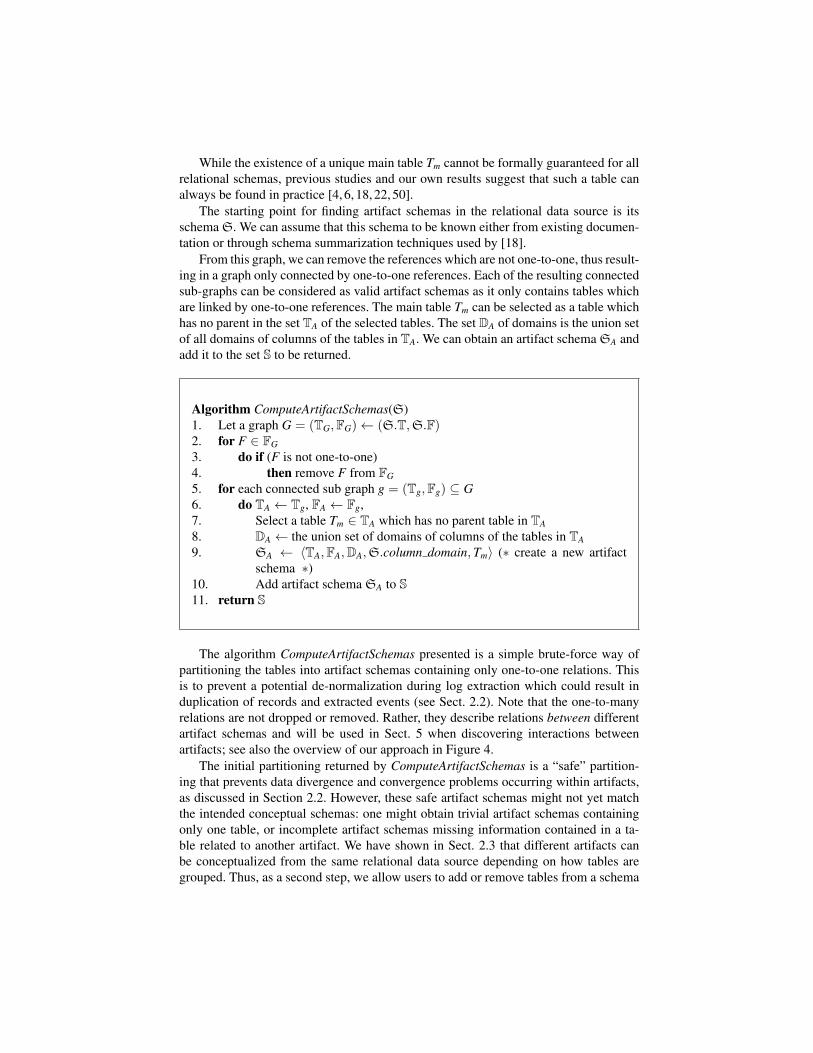
While the existence of a unique main table Tm cannot be formally guaranteed for allrelational schemas, previous studies and our own results suggest that such a table canalways be found in practice [4, 6, 18, 22, 50].

The starting point for finding artifact schemas in the relational data source is itsschema S. We can assume that this schema to be known either from existing documen-tation or through schema summarization techniques used by [18].

From this graph, we can remove the references which are not one-to-one, thus result-ing in a graph only connected by one-to-one references. Each of the resulting connectedsub-graphs can be considered as valid artifact schemas as it only contains tables whichare linked by one-to-one references. The main table Tm can be selected as a table whichhas no parent in the set TA of the selected tables. The set DA of domains is the union setof all domains of columns of the tables in TA. We can obtain an artifact schema SA andadd it to the set S to be returned.

Algorithm ComputeArtifactSchemas(S)1. Let a graph G = (TG,FG)← (S.T,S.F)2. for F ∈ FG

3. do if (F is not one-to-one)4. then remove F from FG

5. for each connected sub graph g = (Tg,Fg) ⊆ G6. do TA ← Tg, FA ← Fg,7. Select a table Tm ∈ TA which has no parent table in TA

8. DA ← the union set of domains of columns of the tables in TA

9. SA ← 〈TA,FA,DA,S.column domain,Tm〉 (∗ create a new artifactschema ∗)

10. Add artifact schema SA to S11. return S

The algorithm ComputeArtifactSchemas presented is a simple brute-force way ofpartitioning the tables into artifact schemas containing only one-to-one relations. Thisis to prevent a potential de-normalization during log extraction which could result induplication of records and extracted events (see Sect. 2.2). Note that the one-to-manyrelations are not dropped or removed. Rather, they describe relations between differentartifact schemas and will be used in Sect. 5 when discovering interactions betweenartifacts; see also the overview of our approach in Figure 4.

The initial partitioning returned by ComputeArtifactSchemas is a “safe” partition-ing that prevents data divergence and convergence problems occurring within artifacts,as discussed in Section 2.2. However, these safe artifact schemas might not yet matchthe intended conceptual schemas: one might obtain trivial artifact schemas containingonly one table, or incomplete artifact schemas missing information contained in a ta-ble related to another artifact. We have shown in Sect. 2.3 that different artifacts canbe conceptualized from the same relational data source depending on how tables aregrouped. Thus, as a second step, we allow users to add or remove tables from a schema

in order to obtain the intended artifacts. This way, also one-to-many relations may beincluded in an artifact schema at the potential cost of data convergence and divergence.Moreover, as one table may contain information of artifacts stored in different schemas(vertical anti-partitioning), we explicitly allow artifact schemas to overlap in tables.

The manual refinement of artifact schemas requires domain knowledge, which istypically available for standard ERP systems by Oracle or SAP. In case no domainknowledge is available, earlier works [18, 44] could be used to automatically identifyartifact schemas based on their informational contents. However, the resulting artifactschemas may include one-to-many relations and thus induce data convergence and di-vergence. Again, a subsequent manual refinement is required to obtain the desired ar-tifact schemas. We illustrate the difference between the original XTract approach [44]and our artifact schema identification using the OTC example. The XTract approachreturns the three artifact schemas shown in the left table of Figure 11 when we set thenumber of artifacts to be 3. Our approach first return three artifact schemas SD, BD,and DD as shown by the black tables in the right table of Figure 11. Since only one in-voice has a change, the document changes table is assigned to the BD artifact schema.The SD artifact schema returned only contains the SD table, similar for the DD artifactschema. Now if users desire to include changes for the SD artifact, they can add thechanges table to the SD artifact schema.

PAGE 33

XTract: Artifact Schemas (k = 3)

Name Main table Tables

BD BD BD

Changes Changes Changes

Changes ? SD, DD

Our Approach: Artifact schemas

Name Main table Tables

BD BD BD, Changes

SD SD SD (, Changes)

DD DD DD

Fig. 11: Comparing the artifact schemas obtained using the XTract approach and ourapproach with respect to tables T and the main table Tm

4.4 Artifact Identification

The tables of an artifact schema SA may contain information about multiple similarartifact types, due to horizontal anti-partitioning. Next, we refine an artifact schemainto its artifact types by specifying discriminating predicates. Also, due to vertical anti-partitioning, the artifact schema may contain attributes that are not relevant for each ofits artifact type. Thus, we project the artifact schema onto only those attributes (identi-fiers, time stamps, etc.) that belong the artifact type.

Definitions Formally, we center the definition of an artifact type around the events de-scribing its life-cycle. Intuitively, each time-stamped value in the data source describesan event, the attribute (or column) containing that value is classified as an event type.That is, an artifact type is a collection of columns containing time-stamp values, and anidentifier. All other columns in the tables of an artifact are considered to be attributesof the various event types where they are accessible for subsequent process mininganalysis. The formal definitions read as follows.

Definition 5 (Event types). Ei = 〈Ename,CEid,Ctime,CEattrs,Econdition〉 ∈ E is an eventtype if and only if:

– Ename is the name of the event type;– CEid is a set of columns defining the event identifier;– Ctime is the column indicating the ordering (or the timestamps) of events of this

event type;– CEattrs is a set of columns denoting the attributes of the event type; and– Econdition is a condition (which can be appended in the FROM part or the WHERE

part of an SQL query) to distinguish various event types stored in the same columnCtime of the data source.

Definition 6 (Artifact types). A = 〈Aname,CAid,E,Cattrs, I,SA,Acondition〉 is an artifactif and only if:

– Aname is and artifact name;– CAid is a set of columns denoting the case identifier of the artifact;– E is a set of event types;– Cattrs is a set of columns denoting the case attributes,– I is a set of interactions between this artifact A and other artifacts (which remains

as an empty set in this section);– SA is the corresponding artifact schema; and– Acondition is the an artifact condition which is an extra condition (which can be

appended in the FROM part or the WHERE part of an SQL query) that is used todistinguish various artifacts having the same main table Tm (or having the sameartifact schema).

We show a concrete example of the artifact definition. Consider the artifact schemaSA = 〈TA,FA,DA, column domain,Tm〉, where the tables TA = {SD} and the refer-ences FA = {〈SD, {SD id}, SD, {Reference id}〉}, we would like to identify two arti-facts, Sales Order and Return Order. Both artifacts may have the same artifact schema,but they could have different events, attributes, and interactions. For example, the ar-tifact Sales Order ASalesOrder = 〈Aname,CAid,E,Cattrs, I,SA,Acondition〉 could have thestructure shown in Table 1, in which each component of the artifact is given a value.

Discovery Algorithms To be able to semi-automatically discover artifacts from an arti-fact schema and a column (or columns) indicating the artifact, we define two functions.The first function constructs a single artifact, whereas the second function constructsmultiple artifacts by calling the first function multiple times.

The first createArtifact(SA, Aname, Acondition) function takes an artifact schema SA,an artifact name Aname, and an artifact condition Acondition as input and returns one arti-fact. For this function, we assume that condition Acondition is given or provided by a userwith insights into the data model of the system. The case identifier CAid of the artifactis defined by the primary key of the main table of the inpu artifact schema SA, eachtime-stamped column Ctime in a table T ∈ TA of the artifact schema defines an eventtype E ∈ E, every other non-time stamped column in T defines an attribute of eventtype E. Every non-time stamped column that cannot be related to one specific event

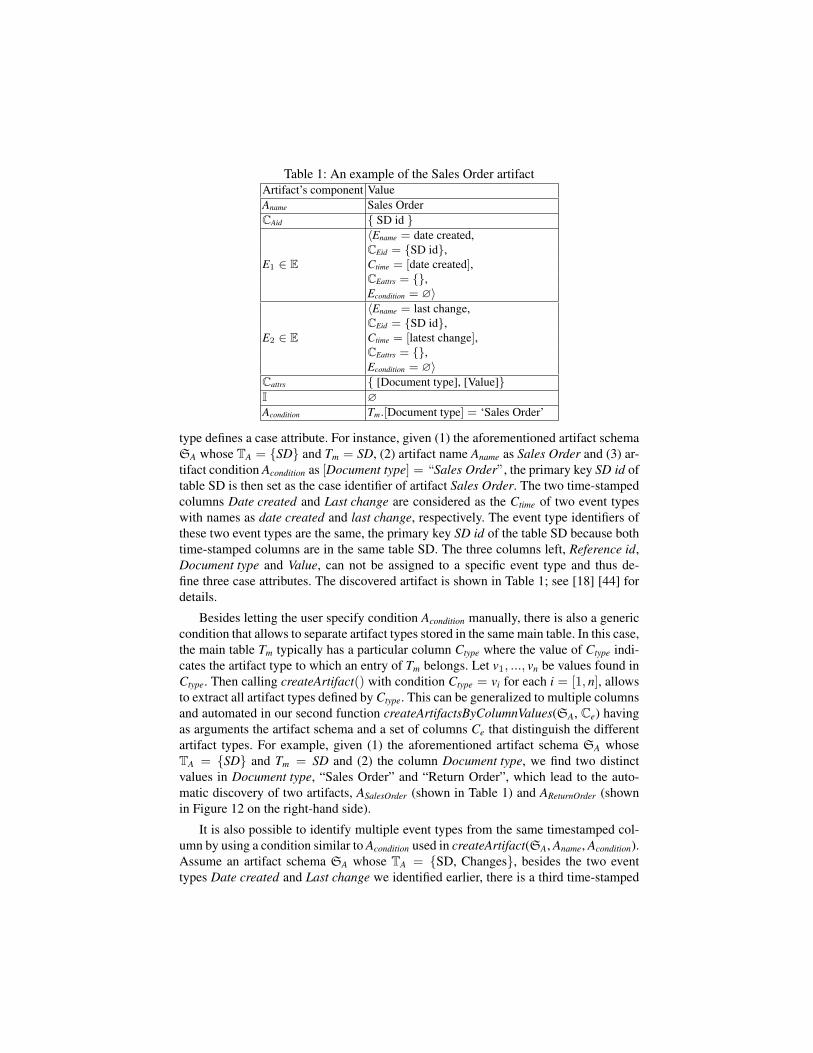
Table 1: An example of the Sales Order artifactArtifact’s component ValueAname Sales OrderCAid { SD id }

E1 ∈ E

〈Ename = date created,CEid = {SD id},Ctime = [date created],CEattrs = {},Econdition = ∅〉

E2 ∈ E

〈Ename = last change,CEid = {SD id},Ctime = [latest change],CEattrs = {},Econdition = ∅〉

Cattrs { [Document type], [Value]}I ∅Acondition Tm.[Document type] = ‘Sales Order’

type defines a case attribute. For instance, given (1) the aforementioned artifact schemaSA whose TA = {SD} and Tm = SD, (2) artifact name Aname as Sales Order and (3) ar-tifact condition Acondition as [Document type] = “Sales Order”, the primary key SD id oftable SD is then set as the case identifier of artifact Sales Order. The two time-stampedcolumns Date created and Last change are considered as the Ctime of two event typeswith names as date created and last change, respectively. The event type identifiers ofthese two event types are the same, the primary key SD id of the table SD because bothtime-stamped columns are in the same table SD. The three columns left, Reference id,Document type and Value, can not be assigned to a specific event type and thus de-fine three case attributes. The discovered artifact is shown in Table 1; see [18] [44] fordetails.

Besides letting the user specify condition Acondition manually, there is also a genericcondition that allows to separate artifact types stored in the same main table. In this case,the main table Tm typically has a particular column Ctype where the value of Ctype indi-cates the artifact type to which an entry of Tm belongs. Let v1, ..., vn be values found inCtype. Then calling createArtifact() with condition Ctype = vi for each i = [1, n], allowsto extract all artifact types defined by Ctype. This can be generalized to multiple columnsand automated in our second function createArtifactsByColumnValues(SA, Ce) havingas arguments the artifact schema and a set of columns Ce that distinguish the differentartifact types. For example, given (1) the aforementioned artifact schema SA whoseTA = {SD} and Tm = SD and (2) the column Document type, we find two distinctvalues in Document type, “Sales Order” and “Return Order”, which lead to the auto-matic discovery of two artifacts, ASalesOrder (shown in Table 1) and AReturnOrder (shownin Figure 12 on the right-hand side).

It is also possible to identify multiple event types from the same timestamped col-umn by using a condition similar to Acondition used in createArtifact(SA, Aname, Acondition).Assume an artifact schema SA whose TA = {SD, Changes}, besides the two eventtypes Date created and Last change we identified earlier, there is a third time-stamped

Name

Artifact Id

Condition

name "Created"

Event id {[SD id]}

Timestamp {[date created]}

Condition

name "last change"

Event id {[SD id]}

Timestamp {[last change]}

Condition

name "Price updated"

Event id {[Change id]}

Timestamp {[Date changed]}

Condition

Changes.[Change type] =

'Price updated'

name "Delivery block released"

Event id {[Change id]}

Timestamp {[Date changed]}

Condition

Changes.[Change type] =

'Delivery block released'

name "Billing block released"

Event id {[Change id]}

Timestamp {[Date changed]}

Condition

Changes.[Change type] =

'Billing block released'

Artifact Sales Order

Sales Order

{[SD id]}

DateCreated

Event type BillingBlockReleased

SD.[Document type] = 'Sales Order'

LastChange

Event type

Event type

Event type PriceUpdated

Event type DeliveryBlockReleased

Name

Artifact Id

Condition

name "Created"

Event id {[SD id]}

Timestamp {[date created]}

Condition

Artifact Return Order

Return Order

{[SD id]}

SD.[Document type] = 'Return Order'

Event type DateCreated

Name Main table Tables

SD SD SD, Changes

Given Artifact schema SDOur Approach

The

origin

al XTract

one schema one artifactone time column one event type

Name

Artifact Id

name "Created"

Event id {[SD id]}

Timestamp {[date created]}

name "last change"

Event id {[SD id]}

Timestamp {[last change]}

name "Changed"

Event id {[Change id]}

Timestamp {[Date changed]}

Event type LastChange

Event type ChangesChanged

Artifact SD

SalesDocuments

{[SD id]}

Event type DateCreated

one schema multiple artifacto

ne

tim

e c

olu

mn

mu

ltip

le e

ven

t ty

pe

s

Fig. 12: Comparing the artifacts obtained using the XTract approach and our ap-proach

column Date changed, which can either be considered as one event type, or we can usethe column Change type to indicate different event type conditions resulting in threedifferent event types (similar to Acondition). An example of the artifact Sales Order wethen discovered is shown in the middle of Figure 12; see [51] for the technical details.Furthermore, the approach presented allows users to add, delete and modify each eventtype, event type attributes and case attributes.

Figure 12 demonstrates the difference in artifacts returned by the XTract approachand our approach. Given the artifact schema SD containing the table SD as the maintable and table Changes, the XTract approach returns one artifact SD shown on the lefthand side in Figure 12. In contrast, our approach allows the user to indicate the columndocument type as a condition column constituting Ce in the function createArtifactsBy-

ColumnValues(SA, Ce). Two artifacts Sales Order and Return Order are then identified,as shown on the right hand side in Figure 12.

4.5 Artifact Extraction

To extract an event log for an artifact, the identified artifact is used to create a logmapping which maps the components of an artifact type to the components of a log.For example, the artifact identifier CAid is mapped to the trace identifier attribute; theevent type identifier CEid is mapped to the event identifier attribute, each timestampcolumn Ctime is mapped to the timestamp attribute. Note that the set of the interactionsof each artifact type is still empty and no information about interactions is mapped norextracted for now.

Next, the log mapping is used to create SQL queries which select the instancesaccording to the log mapping and join the events and attributes to the instances. Theresult of the queries is stored in a cache database, which is then used to write event logfiles in XES format by calling the functions of the OpenXES library3.

Figure 13 shows an example of an event log extracted for the artifact Sales Orderin Figure 12. Only two entries in table SD satisfy the artifact condition SD.[Documenttype] = “Sales Order”, S1 and S2, which respectively result in two traces with S1 andS2 as trace identifiers. According to the event type definitions, we are able to extractfive events for S1 and two events for S2. The corresponding values for the ID, name,timestamp and attributes of an event are also extracted. For example, event e2 of caseS1 is extracted according to event type Price updated and thus has Price updated asname, the value 1 (which is the value of its primary key of column Change id in tableDocuments Changes) as event ID, 17-5-2020 as timestamp (which is the value of col-umn Date changed), and some event attributes extracted from table Documents Changes(as example). Other events are extracted using the same method, see Figure 13.

Our approach basically reused the orginal XTract approach [44] [18] and only ex-tended it by appending the conditions in the WHERE-part of the queries. For technicaldetails, we refer to [51] [44].

Log Name Sales Order

Trace

ID name timestamp event attrs

Event e1 S1 Date created 16-5-2020 -

Event e2 1 Price updated 17-5-2020 Old value = "100", New value = "80"

Event e3 2 Delivery block released 19-5-2020 Old value = "x", New value = "-"

Event e4 3 Billing block released 19-5-2020 Old value = "x", New value = "-"

Event e5 S1 Last change 10-6-2020 -

Trace

ID name timestamp event attrs

Event e1 S1 Date created 17-5-2020 -

Event e2 S1 Last change 31-5-2020 -

ID = S1, Document type = "Sales Order", value = 100

ID = S2, Document type = "Sales Order", value = 200

Fig. 13: An example of event log extracted for artifact Sales Order

3 http://www.xes-standard.org/openxes/start

4.6 Handling Generalization

The previous sections described how to identify and extract artifact types and theirlife-cycle information from a relational data source. The presented steps allowed torevert vertical partitioning, and horizontal and vertical anti-partitioning of the givendata. Here, we discuss how to handle horizontal partitioning in the data source, that is,when information about a conceptual general artifact is not stored as such, but has beendistributed over many different tables. For example in Fig. 1, one could be interested inextracting a general “Documents” artifact rather than one artifact for different documenttypes.

Generalizing different artifact types into one general artifact is similar to generaliz-ing entities and highly depends on the given relational schema [52].

1. The specialization is materialized in the relational schema by a discriminating at-tribute. In this case all artifact types are found in the same tables, and hence willbe contained the same artifact schema. When defining the artifact type, one simplyspecifies are more general discriminating condition Acondition in Def. 6. The result-ing general artifact type then contains more or even all event types and attributes inthe artifact schema.

2. The specialization is materialized as an “IS-A” relationship with a “general table”and foreign keys from its specializations. In this case, the general table and allspecializations of interest become part of the artifact schema, and the general tableis chosen as main table. Artifact type definition proceeds as described above.

3. The specialization is materialized as separate tables without an “IS-A” relation-ship. In this case no generalizing main table for the different specializations can bedefined. Two solutions are possible. (1) One can first extract the life-cycle eventlog for each specialized artifact, and then merge the resulting event logs into onegeneralized event log. Prefixing values of identifier attributes prevents collisionsof different specializations. (2) For the purpose of the analysis, one could trans-form a copy of the original relational source, for example by introducing an “IS-A”relationship with appropriate foreign keys.

4.7 Artifact Life-cycle Discovery

For each artifact Ai which we identified on the database level, we have shown how to ex-tract an event log Li. To discover the life cycle Mi of artifact Ai from the correspondinglog Li, we can reuse existing process discovery algorithms. For discovering a life-cyclemodel from a log Li, generally the same considerations apply as for discovering a pro-cess model from Li. There are various discovery algorithms available and the user hasto pick one that satisfies her desired criteria.

For Life-cycle discovery, we provide no new technique but re-use existing processdiscovery techniques that create from an event log of a process, a process model. Theadvantages and disadvantages of these techniques have been discussed extensively on aconceptual and on empirical level [31]. A user can choose a suitable algorithm based onthese and the desired characteristics and quality criteria with respect to the target model(fitness, precision, simplicity, generalization). Often, different mining algorithms can

be used depending on the purpose, e.g., ILP miner for optimizing fitness and precision,ETM to balance quality criteria, heuristics miner to show a simple model without com-plex routing logic (though without operational semantics), etc. One characteristic thatis specific to artifacts is that, unlike classical workflow processes, concurrency in thediscovered may be of secondary concern (i.e., a business object may never be accessedconcurrently by two users/processes at the same time, thus a transition system model[TS miner] could provide a the right representational bias that does not introduce ar-tificial concurrency). The subsequent interaction discovery requires that each event ofan artifact is translated into (exactly one) action of the life-cycle model as otherwiseinteractions cannot be discovered properly. This assumption excludes algorithms thatmay discard certain events during discovery or that may duplicate tasks.

For the remainder, we assume that Miner(L) denotes some life-cycle miner thatreturns a process model M of the life-cycle of Ai. For the artifact type Sales Orderwe shown in Figure 12 and the event log that we extracted for this artifact shown inFigure 13, we discovered a life-cycle of this artifact shown in Figure 14 by applying theflexible heuristic miner [25].

Fig. 14: The life-cycle discovered for the artifact Sales Order

5 Interaction Discovery

Having identified artifact life-cycles, we can now approach the problem of discoveringinteractions between artifacts. In Section 5.1, we begin with an analysis of the possibleinteractions between artifacts. In Section 5.2, we illustrate how to identify interactionsbetween artifact types and between instances. Enriching the logs extracted for artifactswith these interactions is discussed in Section 5.3. These enriched logs can then beused to identify interactions between event which is discussed in Section 5.4. Finally,Section 5.5 presents the computation of artifact-centric models.

5.1 Interaction Types and Definitions

Interactions between artifacts can be studied from different levels of abstractions. Fig-ure 15 illustrates four levels of interactions: interactions (a) between artifact instances,(b) between artifact types, (c) between events of artifacts, or (d) between event types ofartifacts.

The (a) artifact instance level interactions denotes interactions between two artifactinstances such as the sales order S1 and the return order S3. The (b) artifact type levelinteractions refer to interactions between two artifact types such as the Sales Orderand the Return Order. The existence of interactions between two instances indicates, tosome extent, the existence of an interaction between the two artifact types. The (c) eventlevel interactions are interactions between two events such as the Latest Change eventwith id S1 and timestamp ‘10-6-2020’ of the sales order S1 and the Date Created eventwith id S3 and timestamp ‘10-6-2020’ of the return order S3 that is related to sales orderS1. The (d) event type level interactions denote interactions between two event typessuch as the Latest Change event type of the sales order artifact and the Date Createdevent type of the return order artifact. For the sake of brevity, we also refer to artifactinstance level interactions as instance level interactions and refer to artifact type levelinteractions as type level interactions.

PAGE 27

Artifacts Event types

Artifact instances Events

Specifies

Performed

Instantiation Instantiation

Event type level interactions

Events level interactions Artifact instance level interactions

Artifact type level interactions

Definition

Recording

Indicate

DB level Log level

Artifact LogMapping

Event Log

CacheDB

Indicate

Fig. 15: The four levels of interactions

Direct Type- and Instance Level Interaction Before formally defining interactions,we explain briefly the reasoning behind the existence of interactions. Starting from twogiven artifacts, each of which has a main table containing its instances. If there exists areference between the two main tables and there is an instance in one of the two tables

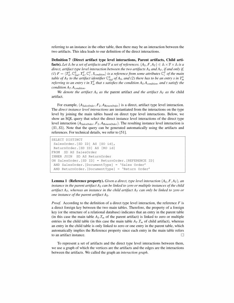
referring to an instance in the other table, then there may be an interaction between thetwo artifacts. This idea leads to our definition of the direct interactions.

Definition 7 (Direct artifact type level interactions, Parent artifacts, Child arti-facts). Let A be a set of artifacts and F a set of references. (AS,F,AT) ∈ A×F×A is adirect, artifact type level interaction between the two artifacts AS and AT , if and only if,(1) F = 〈TS

m,CSAid,T

Tm,CT

c , Scondition〉 is a reference from some attributes CTc of the main

table of AT to the artifact identifier CSAid of AS, and (2) there has to be an entry s in TS

mreferring to an entry t in TT

m that s satisfies the condition AS.Acondition, and t satisfy thecondition AT .Acondition.

We denote the artifact AS as the parent artifact and the artifact AT as the childartifact.

For example, (ASalesOrder,F2,AReturnOrder) is a direct, artifact type level interaction.The direct instance level interactions are instantiated from the interactions on the typelevel by joining the main tables based on direct type level interactions. Below, weshow an SQL query that select the direct instance level interactions of the direct typelevel interaction (ASalesOrder,F2,AReturnOrder). The resulting instance level interaction is(S1, S3). Note that the query can be generated automatically using the artifacts andreferences. For technical details, we refer to [51].

SELECT DISTINCTSalesOrder.[SD ID] AS [SO id],ReturnOrder.[SD ID] AS [RO id]

FROM SD AS SalesOrderINNER JOIN SD AS ReturnOrderON SalesOrder.[SD ID] = ReturnOrder.[REFERENCE ID]AND SalesOrder.[DocumentType] = ‘Sales Order’AND ReturnOrder.[DocumentType] = ‘Return Order’

Lemma 1 (Reference property). Given a direct, type level interaction (AS,F,AT), aninstance in the parent artifact AS can be linked to zero or multiple instances of the childartifact AT , whereas an instance in the child artifact AT can only be linked to zero orone instance of the parent artifact AS.

Proof. According to the definition of a direct type level interaction, the reference F isa direct foreign key between the two main tables. Therefore, the property of a foreignkey (or the structure of a relational database) indicates that an entry in the parent table(in this case the main table AS.Tm of the parent artifact) is linked to zero or multipleentries in the child table (in this case the main table AT .Tm of child artifact), whereasan entry in the child table is only linked to zero or one entry in the parent table, whichautomatically implies the Reference property since each entry in the main table refersto an artifact instance.

To represent a set of artifacts and the direct type level interactions between them,we use a graph of which the vertices are the artifacts and the edges are the interactionsbetween the artifacts. We called the graph an interaction graph.

PAGE 22

Sales Documents

Table

Deliveries Documents

Table

Sales

Documents

table

Deliveries

Documents

table

Billing

Documents

table

Billing Documents

Table

Sales Order Delivery

Return order Return delivery

Invoice

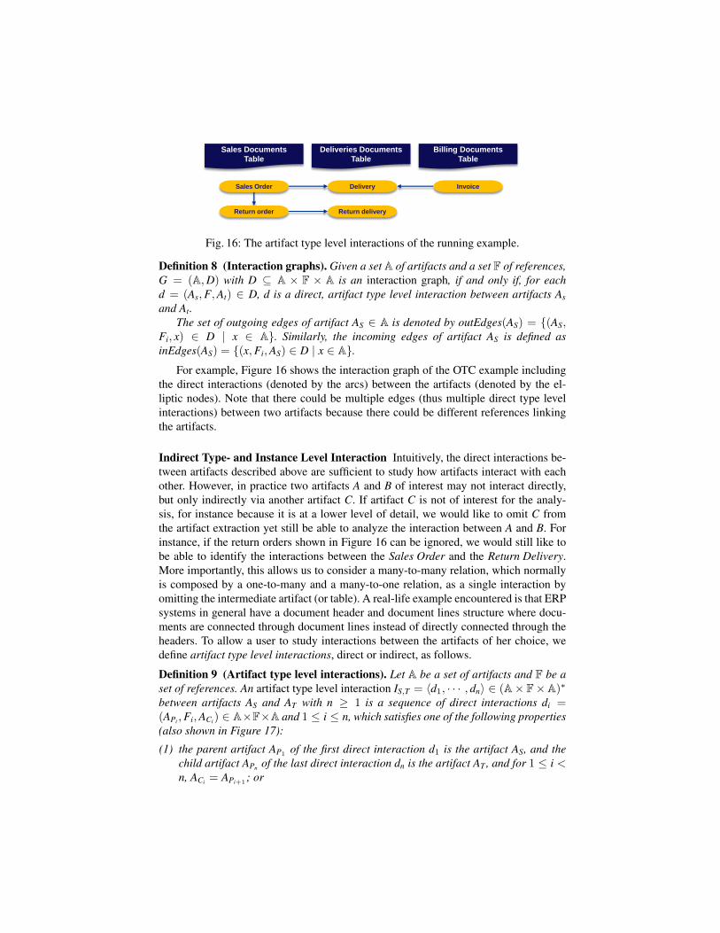
Fig. 16: The artifact type level interactions of the running example.

Definition 8 (Interaction graphs). Given a set A of artifacts and a set F of references,G = (A,D) with D ⊆ A × F × A is an interaction graph, if and only if, for eachd = (As,F,At) ∈ D, d is a direct, artifact type level interaction between artifacts As

and At.The set of outgoing edges of artifact AS ∈ A is denoted by outEdges(AS) = {(AS,

Fi, x) ∈ D | x ∈ A}. Similarly, the incoming edges of artifact AS is defined asinEdges(AS) = {(x,Fi,AS) ∈ D | x ∈ A}.

For example, Figure 16 shows the interaction graph of the OTC example includingthe direct interactions (denoted by the arcs) between the artifacts (denoted by the el-liptic nodes). Note that there could be multiple edges (thus multiple direct type levelinteractions) between two artifacts because there could be different references linkingthe artifacts.

Indirect Type- and Instance Level Interaction Intuitively, the direct interactions be-tween artifacts described above are sufficient to study how artifacts interact with eachother. However, in practice two artifacts A and B of interest may not interact directly,but only indirectly via another artifact C. If artifact C is not of interest for the analy-sis, for instance because it is at a lower level of detail, we would like to omit C fromthe artifact extraction yet still be able to analyze the interaction between A and B. Forinstance, if the return orders shown in Figure 16 can be ignored, we would still like tobe able to identify the interactions between the Sales Order and the Return Delivery.More importantly, this allows us to consider a many-to-many relation, which normallyis composed by a one-to-many and a many-to-one relation, as a single interaction byomitting the intermediate artifact (or table). A real-life example encountered is that ERPsystems in general have a document header and document lines structure where docu-ments are connected through document lines instead of directly connected through theheaders. To allow a user to study interactions between the artifacts of her choice, wedefine artifact type level interactions, direct or indirect, as follows.

Definition 9 (Artifact type level interactions). Let A be a set of artifacts and F be aset of references. An artifact type level interaction IS,T = 〈d1, · · · , dn〉 ∈ (A× F×A)∗between artifacts AS and AT with n ≥ 1 is a sequence of direct interactions di =(APi ,Fi,ACi) ∈ A×F×A and 1 ≤ i ≤ n, which satisfies one of the following properties(also shown in Figure 17):

(1) the parent artifact AP1of the first direct interaction d1 is the artifact AS, and the

child artifact APn of the last direct interaction dn is the artifact AT , and for 1 ≤ i <n, ACi = APi+1 ; or

(2) the child artifact AC1of first direct interaction d1 is the artifact AS, and the parent

artifact APn of the last direct interaction dn is the artifact AT , and for 1 ≤ i < n,APi = ACi+1 ; or

(3) there is a number k and 1 ≤ k ≤ n, for 1 ≤ i < k, ACi = APi+1, and ACk = ACk+1

,and for k < i < n, APi = ACi+1

, and the parent artifact AP1of first direct interaction

d1 is the artifact AS, and the parent artifact APn of the last direct interaction dn isthe artifact AT .

Additionally, in all cases the number of instance level interaction is greater than zero.

PAGE 31

S T d1 dn

S T d1 dn AP1 ACn Ac1

Apn

S d1 dk AP1

ACk = AC(k+1)

T dk+1 dn Apn

(1) (2)

(3)

Fig. 17: Type level interactions

Definition 10 (Strongly connected interactions). The artifact type level interactionsIS,T = 〈d1, · · · , dn〉 between artifacts AS and AT that satisfy the first or the second prop-erties in Definition 9, we called them the strongly connected interactions. The length ofstrong joins of this interaction is n.

Figure 18(a) shows a strongly connected interaction consisting of two direct interac-tions (ASalesOrder,Fi,AReturnOrder) and (AReturnOrder,Fj,AReturnDelivery) linked by AReturnOrder.Since both interactions share the return order artifact, it is possible to join the three maintables based on the two direct interactions. As the references are joined in the same di-rection, we have the guarantee that an instance of the artifact ATi is only linked to zeroor one instance of the artifact ASi , based on the reference property. This property alsoindicates that an instance of the artifact ASi is linked to all related instances of the arti-fact ATj , and these instances of ATj are not linked to any other instances of the artifactASi .

Definition 11 (Weakly connected interactions). The artifact type level interactionsIS,T = 〈d1, · · · , dn〉 between artifacts AS and AT that satisfy the third property inDefinition 9, we called them the weakly connected interactions. The length of strongjoins of this interaction is k, and the length of weak joins is m = n − k. When thelength m of weak joins is greater than zero, the interaction instances could be an over-approximation. We define functions lengthSJ : I → N and lengthWJ : I → N toretrieve the length of strong joins (k) and the length of weak joins (m) of an interaction,respectively.

Figure 18(b) shows a weakly connected interaction comprised two direct interac-tions (ASalesOrder,Fi,ADelivery) and (AInvoice,Fj,ADelivery) linked to the same child artifact

Sales Order

Return order Return delivery

Sales Order Delivery Invoice

Sales Order Delivery

Return order

S1

S3 D4

S1

S2

D1

D2

B1

B2

D3

S1

S3

D1

D2

(a)

(b)

(c)

Fig. 18: The three possible cases of indirect interactions constituted of two directinteractions

ADelivery. The instances of the artifact Sales Order are explicitly linked to the instancesof the artifact Invoice via the instances of the artifact Delivery, as shown by the graphin Figure 18(b) on the right-hand side. For example, S1 linked to B1 via D1, S1 linkedto B2 via D2, and S2 linked to B2 via D3. This explicitness is because an instance ofthe artifact Delivery can only be linked to one instance of Sales Order and one instanceof Invoice (e.g. (S1, D1, B1)) based on the reference property. However, also based onthe reference property, there is the possibility that an instance of the artifact Invoiceis linked to multiple sales orders (e.g. B2). As a result, when the invoices B1 and B2are selected as the indirect instance level interactions for the sales order S1, we havealso included a part of B2 that is not related to S1 but related to S2. Therefore, there isan over-approximation when a weakly connected interaction is used to derive instancelevel interactions.

Invalid Interactions. Compared to weakly connected interactions, sequences thathave two consecutive direct interactions (ASi ,Fi,ATi) and (ASi ,Fj,ATj) with the sameparent artifact ASi and different target artifacts is invalid. Figure 18(c) shows an exam-ple: the interaction composed of (ASalesOrder,Fi,ADelivery) and (ASalesOrder,Fj,AReturnOrder).Since an instance of the artifact Sales Order can be linked to multiple instances of the ar-tifact Delivery and multiple instances of the Return Order, it is impossible to determinethe exact relations between the instances only based on the references. For instance, D1and D2 refer to S1, but also S3 refers to S1, but there is no explicit relation that indi-cates whether D1 is then related to S3 or D2 to S3. Therefore, this type of interaction isconsidered to be invalid.

Possibility of Identifying Event Level Interactions The definition and the examplesdemonstrate that type level interactions and instance level interactions between two ar-tifacts can be identified on the database level. However, the database is not suitable foridentifying event level interactions as we illustrated on our OTC example. The directinteraction between the Sales Order and the Return Order does not indicate whether theDate Created event type of Return Order is (causally) related to the Date Created eventtype of Sales Order or to the Latest Change event type of the Sales Order. Moreover,we aim at identifying a “direction” of interaction such as “event e1 caused event e2”.

This information requires to compare the order of different events in time. For this pur-pose, the event log structure and process mining techniques are much more suitable thanthe tables of a relational database. Therefore, we propose to identify event level interac-tions after we extracted the artifact event logs (which will be discussed in Section 5.4).Though in order to allow finding event level interactions in event logs, we first haveto enrich the event logs (extracted in Section 4) with information about artifact levelinteractions. The algorithms for enriching logs are presented in Section 5.3.

5.2 Artifact Type Level Interaction Discovery

To compute artifact type level interactions, our method consists of two parts. First, givena set of artifacts A = {A1, · · · ,An}, we compute an interaction graph G = (A,D). Fromthe interaction graph G, we then compute a set of type level interactions I, direct andindirect, for each artifact.

Interaction Graph Construction To solve the first part, we introduce the algorithmConstructInteractionGraph(A,F). We first define an auxiliary function Artifacts(T) ={A ∈ A | A.Tm = T} to retrieve a set of artifacts that shares the same main table T .Then, using Artifacts(Tp) and Artifacts(Tc), for each reference F ∈ F between Tp andTc, we retrieve all artifacts Ap that has the parent table Tp and all artifacts Ac of thechild table Tc, respectively (see Line 3). For each combination of Ap and Ac with thereference F between them, we select the count using the countSelect query defined inSection 5.1 to verify whether it is a direct interaction (see Line 4). If the count is greaterthan 0, then an edge (Ap,F,Ac) is added to D as an edge in the interaction graph G.

Algorithm ConstructInteractionGraph(A,F)1. D← ∅2. for F = 〈Tp,Cp,Tc,Cc, Scondition〉 ∈ F3. do for Ap ∈ Artifacts(TP), Ac ∈ Artifacts(Tc)4. do if countSelect(Ap,F,Ac) ≥ 05. then D← D ∪ (Ap,F,Ac)6. return G = (A,D)

Computing Artifact Type Level Interactions To solve the second part, i.e. discov-ering a set of (direct and indirect) interactions for each artifact given, we present thealgorithm CalculatesInteractions(A,G, r, k,m), with r > 0, k ≥ 1 and 0 ≤ m ≤ k,which returns the set A of artifacts, and for each artifact AS ∈ A we fill in the set IS ofinteractions with the following requirements. For each interaction IS ∈ IS, the length ofthe strong joins is at most k, the length of weak joins is at most m and the number ofdistinct instance level of interactions is at least r.

The algorithm CalculatesInteractions runs the following. For each artifact AS ∈ A,it initializes the set I of interactions as empty set. Next, taking AS as the start point, the

algorithm simply explores all paths in the interaction graph G with a depth first strategyby recursively calling the algorithm calculateJoins. The paths that satisfy the require-ments w.r.t. k, m, and r are returned as type level interactions for AS (see Appendix fordetails).

Algorithm CalculatesInteractions(A,G, r, k,m)1. for AS ∈ A2. do I← ∅3. for (AS,F,At) ∈ outEdges(AS)4. do Icurrent ← 〈(AS,F,At)〉5. if countSelect(Icurrent) ≥ r6. then I← I ∪ Icurrent

7. calculateJoins(AS, At, Icurrent, I, r, k − 1, m)8. A.I← I9. return A

After the algorithm CalculatesInteractions(A,G, r, k,m) terminates, we have, foreach artifact A ∈ A, the set A.I of interactions calculated and returned. Users can selecta set of desired type level interactions from the set A.I.

Single-Sided Discovery Note that we made a design decision to restrict the identifi-cation of symmetric interactions on the parent artifact by using the condition that thelength of strong joins is at least the length of weak joins, in addition to that the numberof strong joins greater than zero (i.e. k ≥ 1). In other words, recalling the three situ-ations of type level interaction shown in Figure 17, we only obtain interactions of theparent artifact AS that satisfy (1), or (3) with m ≤ k. The interactions that satisfy (2)or (3) with m > k will only be extracted as the interactions of artifact AT . Note thatthis decision will also effect the event logs we extract. An instance level interaction willonly be extracted for the parent artifact.

There are several advantages to only identify interactions on the one side. First,limiting the interactions to the parent artifact can prevent duplicated attributes to beextracted to improve the performance of log extraction. Furthermore, this decision alsolimits the number of discovered interactions to decrease the number of manual selec-tions that are needed by users. Moreover, we retain the parent and child structure andthe reference property which can be reused during the process discovery. We have ob-served one disadvantage. For example, when a child artifact instance has an interactionwith a parent artifact instance but this parent instance is not extracted in the event log,then we miss the information that the child instance has an interaction in the event log.Changing the proposed algorithm to extract interactions on both side is considered asfuture research.

5.3 Enriched Log Extraction

Using the method described in Section 5.2, we discovered for each artifact a set of typelevel interactions and their instance level interactions. These instance level interactionsare used to enrich logs extracted for artifacts (which is discussed in Section 4.5) andthus retained for the mining phase. The method runs as follows.

Each artifact type level interaction is used to generate an SQL query that joins themain tables of artifacts and select interactions between the artifact instances. These in-stance level interactions are considered as (a list of) attributes of an artifact instance andextracted as the case attributes for the artifact instance. For example, Figure 19 showsthe artifact type Sales Order filled with two type level interactions I1 and I2 (omittedthe five event types in Figure 11 for the sake of brevity). Using similar automaticallygenerated SQL queries as we discussed in Section 5.1, we obtain {(S1, S3)} and {(S1,D1), (S1, D2)} as instance level interactions of sales orders S1 with return orders anddeliveries, respectively. For sales order S2, only interactions with deliveries are found,{(S2, D3)}; the instance level interactions between S2 and return orders is an emptyset. The instance level interactions (stored in the cache database) can now be extractedto enrich the event log of artifact Sales Order. Thus, the log shown in Figure 13 is nowenriched with the three case attributes as Figure 20 illustrated with the highlighted parts(we omitted the events for the sake of brevity). For instance, trace S1 has now two caseattributes additionally: one indicates its interacting traces in the artifact Delivery whichare D1 and D2; another indicates its interacting trace in artifact Return Order which isS3. For technical detail, we refer to [51].

Artifact name

Artifact Identifier

Condition

Interaction I1

Interaction I2

<A_SalesOrder, F1, A_ReturnOrder>

<A_SalesOrder, F2, A_Delivery>

Artifact Sales Order

Sales Order

{[SD id]}

SD.[Document type] = 'Sales Order'

Fig. 19: An example of artifact Sales Order with type level interactions

Log Name Sales Order

Trace

ID name timestamp event attrs

Event e1 S1 Date created 16-5-2020 -

Event e2 1 Price updated 17-5-2020 Old value = "100", New value = "80"

Event e3 2 Delivery block released 19-5-2020 Old value = "x", New value = "-"

Event e4 3 Billing block released 19-5-2020 Old value = "x", New value = "-"

Event e5 S1 Last change 10-6-2020 -

Trace

ID name timestamp event attrs

Event e1 S1 Date created 17-5-2020 -

Event e2 S1 Last change 31-5-2020 -

Log Name Sales Order

Trace

Events ID name timestamp event attrs

Trace

Events ID name timestamp event attrs

ID = S1, Document type = "Sales Order", value = 100

ID = S2, Document type = "Sales Order", value = 200

ID = S1, Document type = "Sales Order", value = 100

ID = S2, Document type = "Sales Order", value = 200

Interaction_Delivery = {D1, D2}, Interaction_ReturnOrder = {S3}

Interaction_Delivery = {D3}

Fig. 20: An example of event log extracted for artifact Sales Order with instancelevel interactions as case attributes

5.4 Event Type Level Interaction Discovery

We have shown how to identify type level interactions and enrich the logs with trace at-tributes of which instance interacts with which other instances. From a log perspective,

a trace t1 of artifact A1 referring to a trace t2 of artifact A2 means that some of the eventsin t1 interact with some of the events in t2. In the following, we present techniques toidentify these interactions between events and event types. First, we retrieve for anytwo artifacts A1 and A2 the pairs of interacting traces. Then, we provide two differentkinds of techniques to identify patterns of possible event interactions between the inter-acting traces of A1 and A2. From these, we then derive event type level interactions. Inparticular we distinguish frequent interactions and infrequent interactions (outliers).

Preliminaries - Event logs We use the formal definition of event log in [1]. In general,an event log comprises a list of traces of which each trace contains all events thatoccurred in a case, i.e., an execution of the process.

Definition 12 (Event universe E). Let E be the event universe, i.e. the set of all possibleevent identifiers. Events may be characterized by various attributes. Let AN be a set ofattribute names. For any event e ∈ E and name n ∈ AN : #n(e) is the value of attributen for event e. If event e does not have an attribute named n, then #n(e) = ⊥ (nullvalue).

For example, #type(e) is the event type associated to event e describing the activitythat has been executed; #time(e) is the timestamp of event e (also denoted by T (e)).

Definition 13 (Case universe L). Let L be the case universe, i.e. the set of all possiblecase identifiers. A case also has attributes. For any case c ∈ L and name n ∈ AN :#n(c) is the value of attribute n for case c. If case c does not have an attribute namedn, then #n(c) = ⊥.

Definition 14 (Traces). Each case has a special mandatory attribute trace: #trace(c) =σc ∈ E∗, which is a finite sequence of events σ ∈ E∗ such that each event appears onlyonce. We assume traces in a log contain at least one event, i.e. #trace(c) 6= 〈〉.

Definition 15 (Logs). An event log is a set of cases L ⊆ L such that each event appearsat most once in the entire log. We use A to denote the set of all event types appearingin log L, i.e. A = {#type(e) | c ∈ L ∧ e ∈ #trace(c)}.

We also define the following short notations for your convenience.

Definition 16 (Projection F). Given a log L and an event type E ∈ A, FE(L) filters Land retain, for each of its traces, the event of event type E only.

For example, the trace sales order σS1 consists of two events, i.e. 〈(S1, created,16-5-2020), (S1, latestchange, 10-6-2020)〉. If we apply the project function on the traceσS1 with E = created, we obtain Fcreated(σS1) = 〈(S1, created, 16-5-2020)〉.

Definition 17 (Trace precedence <T ). Given two traces σs and σt, σs <T σt, if andonly if, for each event es ∈ σs and et ∈ σt, the timestamp #time(es) of the event es isbefore the timestamps #time(et).

For example, FE(σs) <T FE(σt) means that each event es ∈ σs which has the eventtype E is executed earlier than each event et ∈ σt which has the event type E. σs =T σt,σs >T σt, σs ≤T σt and σs ≥T σt are also similarly defined.

Interacting Traces We define a function #I T(cs) which returns the set of the instancelevel interactions of case cs with the cases in artifact T .

Definition 18 (Function #I T(c)). Given a log L, of which each case is enriched withinstance level interactions, a case c, and artifact T, we use the notation #I T(c) toretrieve the instance level interactions between the case c and the set of cases of artifactT.

If we use the log shown in Figure 20 as an example, #I Delivery(S1) = {D1,D2},#I ReturnOrder(S1) = {S3}, and #I Delivery(S2) = {D3}. If the case has no interactionwith the given artifact, an empty set is returned, e.g. #I ReturnOrder(S2) = ∅.

Definition 19 (Function I). Given two event logs LS and LT , we define I(LS,LT) ={(cs, ct) | cs ∈ LS ∧ ct ∈ LT ∧ ct ∈ #I T(cs)} ⊆ LS × LT as the set of trace levelinteractions between the logs LS and LT , where each (cs, ct) ∈ I(LS,LT) indicates thatthere is an instance level interaction between the two traces cs and ct seen from theparent artifact AS to the child artifact AT .

We illustrate the function I with the OTC example shown in Figure 18(b). Assumewe have extracted an event log of the artifact Sales Order with trace level interactions tothe artifact Invoice and an event log of the artifact Invoice (i.e. the artifact Sales Orderis the parent artifact). We use the trace id to represent the trace. Thus the set of tracelevel interactions I(LSalesOrder,LInvoice) = {(S1,B1), (S1,B2), (S2,B2)}.

Definition 20 (Event type level interactions (ETLI)). Given two artifact types AS andAT , and their set of event types AS and AT , respectively, an event type level interaction(ap, ac) between AS and AT satisfies, at least, the requirement that ap ∈ AS and ac ∈AT , or vice versa.

In the following, we present two methods to identify event type level interactionsbetween the events of two interacting traces LS and LT . More specifically, we identifythe relation X ⊆ (AS ×AT) ∪ (AT ×AS) where AS and AT denote the event types ofLS and LT , respectively.

ETLI Discovery by Merging Logs The first idea for discovering event type levelinteractions is to compute a merged trace from any two interacting traces of artifactsA1 and A2 (by putting all their events in one trace). Doing this for all interacting tracesgives a merged log. Applying a classical process discovery algorithm then allows toidentify causal dependencies between activities from artifacts A1 and A2. These can beinterpreted as event type level interactions between A1 and A2.

We present the CalcETLInteractionsByMergingLogs algorithm below. In general,for each (σs, σt) ∈ I(LS,LT), we merge the two traces to a new trace using the mergefunction M (see Line 5) that simply builds the union of the events of two traces σs

and σt and orders all events by their timestamp (see [51] for a formal definition). Allmerged traces are added to the log Lnew containing events originally from two artifacts.Now, a process discovery algorithm Miner() can be applied on the merged log Lnew todiscover dependencies between the two sets of event types, i.e.AS andAT . (see Line 7).

Each direct succession (Ei,Ej) between the two event types Ei and Ej discovered whereEi ∈ AS and Ej ∈ AT (or vice versa) is considered an event type level interactionbetween artifacts AS and AT , and added to the result X (see Lines 8-9).

Algorithm CalcETLInteractionsByMergingLogs(LS,LT )1. if I(LS,LT) = ∅2. then return ∅3. else Lnew ← [], X ← ∅4. for (σs, σt) ∈ I(LS,LT)5. do σnew ←M(σs, σt)6. if σnew 6= 〈〉 then add σnew to Lnew

7. Mnew ← Miner(Lnew)8. for (Ei,Ej) where Ej is a direct successor of Ei in the model Mnew, and

(Ei,Ej) ∈ AS ×AT or (Ei,Ej) ∈ AT ×AS

9. do add (Ei,Ej) to X.10. return (Lnew,X)

For example, if we use the heuristic miner as the Miner(Lnew), a simple causality netDG = (Anew,D), in which D ⊆ Anew × Anew indicates the direct succession betweenevent types, is obtained from the log Lnew. Here, a dependency (Ei,Ej) ∈ D with Ei ∈ALS and Ej ∈ ALT (or vice versa) is returned as an event type level interaction. Whenusing a miner that returns a Petri net, we first compute the direct succession betweentransitions by omitting the places and then identify event type level interactions.

An important remark is that different process discovery techniques return a differ-ent set of event type level interactions. The meaning of an event type level interactionsidentified also varies depending on the discovery miner chosen as Miner(L). For ex-ample, the interactions (dependencies) between two event types identified by the alphaminer are absolute precedence, thus event type A always before event type B, and noB is found before A in the log. In contrast, the event type level interactions returned bythe flexible heuristic miner have a different meaning, i.e. event type A is mainly beforeevent type B, and B before A is much less frequent (or lower than the threshold) in thelog.

ETLI Discovery by Using Defined Criteria Using an existing miner to identify in-teraction may not be feasible in all situations. In particular the miner might producemodels of low quality on the given data, or the user might not be interested in all in-teractions, but only in a specific subset. For such situations, we introduce a differentmethod for identifying event type level interactions based on a simple precedence ofevents and time intervals between directly succeeding events. This method allows toconsider all possible interactions (including outliers) or filter interactions based on awell-defined criterion.

We define several criteria, and for each criterion, a suitable situation is given as anexample to use this criterion. For all criteria, let LS,LT be two logs with event types AS

and AT respectively, and | I(LS,LT) |> 0. Further, assume a user selected subsets ofevent types with AsubS ⊆ AS,AsubT ⊆ AT . We would like to find a set X of event typelevel interactions betweenAsubS andAsubT such that one of the following criteria holds.

Definition 21 (Criterion absolute precedence). For each (Ep,Ec) ∈ AsubS × AsubT ∪AsubT × AsubS, (Ep,Ec) ∈ X is an ETLI according to absolute precedence, iff, for all(σs, σt) ∈ I(LS,LT) : FEp(σs) ≤T FEc(σt)

The criterion absolute precedence basically says that in every trace any event oftype Ep happens before any event of type Ec, without any exceptions.

It is possible that there might be exceptions. For example, the event type Createdof sales orders should always happened before the event type Created of the relateddeliveries, but the recorded data may have been entered manually, and therefore, somedeliveries are created before the creation of orders (and other events could happenedbetween). To be able to detect both the “majority flow” and the “minority flow”, wedefine the existing precedence criterion which says that there exists a trace where Ep ispreceded by Ec.

Definition 22 (Criterion existing precedence). For each (Ep,Ec) ∈ AsubS × AsubT ∪AsubT × AsubS, (Ep,Ec) ∈ X is an ETLI according to existing precedence, iff, there is(σs, σt) ∈ I(LS,LT) : FEp(σs) ≤T FEc(σt)

From a time perspective, we also consider event types that always happen shortlyafter each other, i.e. the average time duration between the events of the two event typesare shortest. We call this the shortest time criterion.

Definition 23 (Criterion shortest time). (Ep,Ec) ∈ X is an ETLI according to shortesttime, iff, (1)

min (Ep,Ec)∈AsubS×AsubT (∑

(σs,σt)∈I(LS,LT ) AvgTimeDur(FEp (σs),FEc (σt))

|I(LS,LT)| )

or (2)

min (Ep,Ec)∈AsubT×AsubS(∑

(σs,σt)∈I(LS,LT ) AvgTimeDur(FEp (σs),FEc (σt))

|I(LS,LT)| )

Note that in each pair of interacting logs, there is only one pair of events with ashortest time interval. Despite this limitation, we found this criterion in our case studies(see Section 7) to be very effective in identifying the main event type level interactionsand hiding the complexities of interleaving relations between artifacts.

In addition, we define event level interactions using merged traces, based on whichwe then introduce the criterion existence of an event level interaction, which to someextent indicates the set of all possible event type level interactions.

Definition 24 (Event level interactions). Let σ = 〈e1, e2, · · · , en〉 be a trace. For alli = [1, ..., n − 1], we call event ei+1 the direct successor of ei; we write (ei, ei+1) ∈

succ(σ). Let succ(L) denote the direct successors of all traces in L. Now, if L is mergedfrom two logs LS and LT (using the function described in Section 5.4), an event ei ∈ Lindicates ei ∈ ES ∪ ET which is the union set of events of LS and LT . We define an eventlevel interaction as follows. A succession (ei, ei+1) ∈ succ(L) with L merged from LS

and LT is an event level interaction between the two events if and only if ei ∈ ES andej ∈ ET or vice versa.

The criterion existence of an event level interactions states if there exists an eventlevel interaction (ei, ei+1) between two event types Ec and Ep, we consider (Ep,Ec) asan event type level interaction.

Definition 25 (Criterion existence of an event level interaction). (Ep,Ec) ∈ X is anETLI according to existence of an event level interaction, iff, there exists (ei, ei+1) ∈succ(L) such that (1) ei ∈ ES ∧ ei+1 ∈ ET (or vice versa) and (2) #type(ei) = Ep ∧#type(ei+1) = Ec

The criterion max number of event level interactions explicitly count how often anevent level interaction occurs in the merged log and treat the maximal interactions.

Definition 26 (Criterion max number of event level interactions). (Ep,Ec) ∈ X is anETLI according to max number of event level interactions, iff, , iff,

max (Ep,Ec)∈AsubS×AsubT

⋃(σs,σt)∈I(LS,LT)

(

{(ei, ei+1) | (ei, ei+1) ∈ σ ∧ σ ∈M(σs, σt)

∧#type(ei) = Ep ∧#type(ei+1) = Ec})∨

max (Ep,Ec)∈AsubT×AsubS

⋃(σs,σt)∈I(LS,LT)

(

{(ei, ei+1) | (ei, ei+1) ∈ σ ∧ σ ∈M(σs, σt)

∧#type(ei) = Ep ∧#type(ei+1) = Ec})

Identifying Unusal Interactions The two techniques introduced in Sections 5.4 and 5.4are designed to identify the artifact interactions. However, a user might also be in-terested in particularly finding outliers, i.e., deviations from the main flow. Next, wepresent a corresponding technique based on the merged event logs of Section 5.4.

To identify outliers in the interaction, we first consider all event level interactions(see Definition 24), thus the directly succeeding events (ei, ei+1) in a merged log. Usingthese event level interactions, we can identify outliers as follows. On the merged log L,we first consider all pairs of event types (of AS and AT ) that directly follow each otherin some trace of L. Then we identify the main interactions between AS and AT by ap-plying a suitable discovery algorithm on the merged log (the technique of Section 5.4).Removing these main interactions from the set of all found direct successors yields theinfrequent interactions. The formal definitions are as follows.

Let the set Xall denote the event type level interactions identified based on the theexistence of an event level interactions criterion (which have included, to some extent,all possible type level interactions), and let Xmain denote the event type level interactionsthat we identified by applying a miner on the merged log. Since we assume the minersidentify the main flows, we consider Xall\Xmain as the set of unusual event type levelinteractions (i.e. outliers).

5.5 Artifact-centric Model Discovery

We have shown two different methods to compute a set X ⊆ AS × AT ∪ AT × AS ofevent type level interactions from two given event logs LS and LT . In this section, wediscuss how to discover an artifact-centric model.

Proclet System Discovery Formally, given a set of event logs {L1, · · · ,Ln}, let a set Mbe the set of life-cycles discovered, i.e. each Mi ∈M is a (Petri net) model describes thelife-cycle of event log Li extracted for artifact Ai. Given two life-cycles MS,MT ∈ M,we can use a mapping function X : (M × M) → A × A to return a set X of eventtype level interactions between the two life-cycles (using our techniques in Sections 5.4and 5.4), i.e. X ⊆ AS × AT ∪ AT × AS. In addition, for each model Mi, we have afunction ATi : Ai → Tiv that maps an event type to the corresponding labeled transitionin the model. To express the identified interactions between these life-cycle models,we turn each model into a proclet and add ports and channels between transitions thatdescribe interacting event types.

We define the constraint that each port is connect to one transition, and each transi-tion is only connect to one input port and one output port. This constraint is due to thefact that when a transition is connected to two output ports, there is no explicit expres-siveness (identifiable) to distinguish whether a message is sent via both output ports(AND-splits), or it is only sent via one output port depending on a condition.

First, we create ports for each model MS ∈ M as follows. Given a model MS repre-senting the life cycle of artifact AS, let XS =

⋃Mi∈M X (MS,Mi) denote all interactions

that AS has with all other artifacts. For each event type Eout of the artifact AS if there isan event type level interaction (Eout,Ei) ∈ XS and (Eout,Ei) ∈ AS × Ai, we create anoutput port for the labeled transition ATs(Eout) in model Ms. For each event types Ein ofMs, if there is an event type level interaction (Ei,Ein) ∈ Xs and (Ei,Ein) ∈ Ai ×As, wecreate an input port for the transition ATs(Ein) in model net Ms.

Finally, we connect the output port of transition AT(Ei) to the input port of transitionAT(Ej) for each distinct type level interaction (Ei,Ej) ∈ X =

⋃Mi∈M,Mj∈M X (Mi,Mj).

Simple Representation To be able to support business users by using our approach,interviews have be conducted within KPMG to investigate the requirements of clientsfor a suitable visual representation. The result of the investigation indicates that theproclet notation might be too formal to be communicated with a non-technical processstakeholder. One of the customers involved in the case study also indicated that he isless interested in the notions of places, tokens, silent transitions, AND-splits and OR-splits and finds the sequential relations containing adequate information. Therefore, we

developed a simpler notation to visualize the life-cycles and their interactions, whichis similar to a simple dependency graph. We obtained this simpler representation byomitting the places of the Petri net and the ports of the system and directly connectingthe transitions with their successors. Examples are shown in Figures 25 and 3.

Complexity Analysis In this section, we provide a complexity analysis of our ap-proach. The running time of algorithms are summarized in Table 2. We use the samenumber to refer to the same step in the overview shown in Figure 4.

In the following analysis, we use | T | to denote the number of tables, | C | todenote the number of columns, | F | the number of references, | A | the number ofartifact types, | E | the number of event types, and | L | to denote the size of log in termof number of events.

The database schema identification (1.0), including primary key and foreign keyextraction, is an NP-hard problem. Our approach and tools support both importing theexisting data schemas, which takes O(| T | + | F |), as well as using the original XTractapproach to discover data schemas, which is exponential in number of columns.

The artifact schema identification (1.1) runs in linear with respect to the number oftables or the number of references. The artifact identification (1.2), which follows, runsin worst case O(| A | × | C |) because for each artifact type the algorithm has to includeall columns (as identifiers, event types, or attributes of the artifact type). The extractionof a log of a defined artifact type (1.3) currently takes quadratic in terms of the numberof entries in the data set, in worst case, since each entry in the main table is joined withall other entries to obtain its events and attributes. In theory, this running time can beimproved to be linear in terms of the number of entries. Finally, the complexity of thediscovery of a life-cycle of an artifact (1.4) depends on the discovery algorithm selected,which might be linear or exponential in terms of the number of events of the log for theartifact.

For discovering interactions between artifact types (2.1), the algorithm basically fol-lows a depth-first-search to select all paths composed of references of which the numberof strong joins is at most k and the number of weak joins is at most m, and therefore,grows exponentially in (k + m). The interactions between artifact types are then usedto extract interactions between artifact instances for logs (2.2), which takes quadratic interms of the number of entries in the data set and is executed during step 1.3. Discover-ing interactions between event types (2.3) of two interacting artifacts requires to mergetheir logs, which takes O(| L |2), to run a discovery algorithm. To discovery an artifact-centric model, step 2.3 is re-run for every two interacting artifacts, and between eachtwo event types, thus O(| E |2), if they interact, we add an event type level interaction.

During the case studies, which is discussed in Section 7, steps (1.3) combined with(2.2) are the most time-consuming part; to extract about 30000 traces, in total circa30000 events, it takes almost a hour. Other steps executed during the two case studiestake less than ten minutes4.

4 We import the data schema, and for step (2.1) we use k = 2 and m = 1

Table 2: Running time analysisStep Running time1.0 NP-hard or O(| T | + | F |)1.1 O(| T | + | F |)1.2 O(| A | × | C |)1.3 O(| Entries |2)1.4 running time on the discovery algorithm selected2.1 O(| A | × | F |k+m)2.2 O(| Entries |2)2.3 O(| L |2 + running time of discovery algorithm)2.4 O(| E |2)

6 Artifact-Centric Process Mining Methodology

In this section, we explain our methodology for conducting an artifact-centric processanalysis project, which we also employed during our case studies. Figure 21 showsthe methodology and indicates which parts of the methodology is supported by ourapproach and implementation.

An artifact-centric process analysis project starts with selecting a data source to beanalyzed, and users can import the data source and data schema using our approach;XTract [18] can be used to automatically discover an unknown data schema. After im-porting the data source, users can discover, create and modify artifact schemas, theirartifacts and interactions between them based on the methods described in Sections 4.3,4.4 and 5.2. Once the artifacts and the interactions between them are specified, ourtechniques can automatically extract an event log for each artifact, as shown in Sec-tions 4.5 and 5.3. The logs are used to discover an artifact-centric process model thatshows the life-cycle of each artifact and the interactions between the artifacts duringtheir life-cycle, which are discussed in Sections 4.7, 5.4 and 5.5. Domain experts canuse this model to analyze and evaluate the business processes in its context and refinethe artifacts, their event types and their interactions if desired. It is common practice inprocess analysis to refine the analysis and data extraction in several iterations.

During the case study, we obtained some best practices with respect to constructingand evaluating an artifact-centric model. To start with, it is much easier to first createan overview of simple artifacts, each of which has only one or two event types (e.g.only Created), and with no more than two interactions between any two artifacts,to help both analysts and clients to start the analysis and to understand the main flowof the process. Moreover, such a simple overview can be used to communicate betweenstakeholders, to further elaborate on requirements and questions, and to find more fine-grained or more complex artifacts. For example, in Section 2.3, the example of theartifact-centric model shown in Figure 3 is much easier to understand than the otherthree. This observation is also verified later during the case study for the Oracle ProjectAdministration process when we tried to communicate with the clients for the first time.

Generally, with respect to evaluating artifacts, we suggest to have simple artifactsand to include only one-to-one relations within artifacts, with one exception: if theentries in the table (to which the artifact’s main table is related via a one-to-many rela-tion) can not be considered as instances of any other artifacts but purely denoting events.

Data source

Artifact schemas / Artifact types

Logs +

Interactions

Artifact-centric models

Refine Artifacts

Evaluate

Repository of schemas

Discover Extract

Good to use

Import / Discover

Where our approach supports

Objects

Methods

Fig. 21: The methodology used for conducting artifact-centric process analysisprojects

For example, the change tables in SAP (CDHDR and CDPOS) only contain events thatdescribe the changes of artifact instances, then it is harmless to include them as eventsof the artifact. Otherwise, it is better to consider the table as a separate artifact.

With respect to discovering and evaluating interactions between artifacts, we discussthe following cases which we learned during our Oracle case study (discussed in Sec-tion 7.4). When the artifacts in a model are clear and simple (e.g. less than two events),one can use the merged traces method to use discovery algorithm to discover the mainevent type level interactions. However, when the complexity of artifacts increases, theinteractions discovered using this method are too complex to start with business users.In this situation, it is better to start with one of the criteria that only result in at mosttwo interactions between artifacts (e.g. Definition 23 criterion shortest time). After themain flow of the model is understood, analysts can use discovering all interactions andoutliers to inspect infrequent or abnormal flows individually.

To refine or evaluate artifacts and their interactions, if an artifact appears to beinteresting, one can start to unfold / extend the artifact by adding more tablesand include more event types. These event types are then also taken into accountwhen discovering interactions. An example of extending simple artifacts is discussedusing the SAP case study in Section 7.3. As a general rule, we found that two eventtypes should only be included in the same artifact type if one wants to comparethe order of their occurrence on the same time-line, for example, if we want toknown when deliveries and return orders happened during the life-cycle of a sale-order.Generally, the definition and refinement of artifact types should orient along theintended conceptual business objects; a domain expert should validate the scope ofthe extracted business objects, a data expert can help in refining the artifact definitionin order to retrieve the intended schema from the relational data source as explained inSection 4. To summarize, we suggest to start analyses with simple, clear artifacts andinteractions and then gradually extend the artifacts and include more interactions whilefocus on the interesting observations made using discovered artifact-centric models.

7 Empirical Evaluation

We implemented the techniques presented in Sections 4 and 5. In this section, we brieflydescribe our implementation and then describe two real-life case studies where this toolwas used.

7.1 Prototype Implementation

Our implementation consists of two parts. A standalone tool which is an extensionof XTract [18] and implements the techniques described in Sections 4 and 5 for dis-covering artifact types and interactions between the artifact types, and for extractinglife-cycle logs that are enriched with information about interactions between artifact in-stances. The tool reads as input the contents of a relational database. Then the user canimport or automatically discover artifact schemas; for each schema the user can spec-ify various artifact types choosing which events and attributes to include. Similarly, allvalid artifact interactions are computed and the user selects the interactions of interest.From this selection one event log per artifact type is extracted containing the artifact’slife-cycle and its interactions to other extracted artifacts.

The second part of our implementation is a plugin to the Process Mining toolkitProM5. The plugin takes as input a set of extracted life-cycle logs. Then, a life-cyclemodel is discovered for each artifact and the user can choose which method to usefor discovering artifact interactions. The resulting life-cycle models with interactionsare shown graphically to the user on a screen where she has various filtering optionsavailable, for instance to highlight outliers. See [51] for details.

7.2 Case Study Design

The goal of the case studies was to evaluate the feasibility and practicability of ourapproach in a real-life setting. More specifically, we wanted (1) to verify whether ourapproach can indeed discover an artifact-centric process model including interactions ina practical setting as a proof-of-concept and (2) avoid false positive flows that showedup in earlier approaches because of convergence and divergence (see Section 2.2). Fur-thermore, we wanted to evaluate whether (3) the discovered model and interactions canprovide accurate data- and facts-based insights of the given data source helping a busi-ness analyst to analyze the process and (4) whether the discovered models can be usedto communicate with and understood by process stake holders with ease.

The first case study was performed in the Order to Cash (OTC) process of SAP.In this case study, we emphasized on the execution of our approach such as decisionsabout the artifact selection and interaction selection since no customer was involved.The second case study was conducted in the Project Administration (PA) process ofOracle. Since real customers were involved, we emphasize the discussion of the resultof analyses.

For each case study, we (1) introduce the process and the data source, (2) explain theexecution of our approach including decisions made, and (3) discuss observations and

5 www.promtools.org

results we have obtained. In addition, during the first case study, we compare our artifactdiscovery to the one used by the original XTract approach, and we show some statisticsabout the false-positive flows with respect to a classical log conversion approach.

7.3 Case I - SAP Order To Cash Process

The first case study was performed for the Order to Cash (OTC) process supportedby SAP systems. The data has been provided by KPMG. The main goal of this casestudy was to evaluate the technical abilities of our technique. Thus, the authors with anaffiliation to KPMG, who are the experts in ERP systems and data analytic and haverich experience of conducting advisory projects for clients, provided the requirementsand evaluated the results based on their experiences in earlier projects.

SAP OTC process and data structure A default OTC process in SAP starts with cre-ating a sales order. After the order is delivered, a delivery document is created. Then, aninvoice document is created in the system, sent to customer and posted in the accountreceivable (table). After receiving the payment, this default OTC process ends. How-ever, there are many complex variations of this process. For example, the orders couldbe linked to a contract document, or return orders could be placed and return deliveriesare made. Credit memo requests might be received from customers when the goods areincomplete or damaged. Invoices might also be canceled.

The data structure used to support the OTC process allows flexibility to deal withthe aforementioned variance, but it is also very complex. The relational data structureof SAP regarding the relevant tables of this case study is discussed in [51].

SAP OTC - Extraction and Discovery In this section, we emphasize the steps takenand decisions made to obtain an artifact centric model for the SAP - OTC process.

Table

Name Constraint and Time scope

Row Count

used

Column

Count

BKPF where '2012-09-01' <= cpudt and cpudt < '2012-11-01' and awtyp = 'vbrk' 11358 32

BSID where '2012-09-01' <= cpudt and cpudt < '2012-11-01' 4428 49

BSAD where '2012-09-01' <= cpudt and cpudt < '2012-11-01' 911 49

CDHDR

where '2012-09-01' <= [UDATE] and [UDATE] < '2012-11-01' and (

cdhdr.objectclas = 'VERKBELEG' or cdhdr.objectclas = 'faktBELEG') 13903 9

CDPOS

inner join cdhdr on cdhdr.changenr = cdpos.changenr where '2012-09-01' <=

[UDATE] and [UDATE] < '2012-11-01' and ( cdhdr.objectclas = 'VERKBELEG' or

cdhdr.objectclas = 'faktBELEG') 56018 10

DDFTX where tabname = 'vbak' or tabname = 'vbrk' 237 5

VBAK where '2012-09-01' <= erdat and erdat < '2012-11-01' 3383 40

VBAP where '2012-09-01' <= erdat and erdat < '2012-11-01' 4317 35

VBRK where '2012-09-01' <= erdat and erdat < '2012-11-01' 5285 37

VBRP where '2012-09-01' <= erdat and erdat < '2012-11-01' 10206 31

LIKP where '2012-09-01' <= erdat and erdat < '2012-11-01' 11623 51

LIPS where '2012-09-01' <= erdat and erdat < '2012-11-01' 13157 15

Fig. 22: SAP OTC process - tables and record counts

First, we imported 11 tables shown in Figure 22 in which the name of the tables, theconstraint for selective import, the number of records used, and the number of columnsare described. We considered only the documents created between ‘01-09-2012’ and

‘31-10-2012’. As some time columns in the OTC process data were not recorded, weonly considered ‘date-stamps’. Primary keys and foreign keys where imported based ondomain knowledge [51].

Second, we observed in the data that documents (e.g. a sales order) and lines (e.g.line items in a sales order) are stored separately in different tables. Moreover, the line-level objects have their own life-cycles which could be independent of the related doc-ument objects. For example, a line item might be rejected but the sales order is stillpursued. As the line objects have many-to-one relation with their related document ob-jects (e.g. a sales order can have multiple sales lines), documents and lines were splitinto separated artifact schemas (automatically done by the algorithm in Section 4.3),leading to 8 artifact schemas in total. For the sales documents (i.e. table VBAK) andlines (i.e. table VBAP), delivery documents (i.e. table LIKP) and lines (i.e. table LIPS),and invoice documents (i.e. table VBRK) and lines (i.e. table VBRP), there is a columnvbtyp in the document tables that indicate the type of documents. Therefore, we createdthe artifacts of documents and lines based on the values found in this column. In total,we identified 35 artifacts. Figure 23 shows some example of the artifact schemas andthe artifacts we identified. The complete list can be found in [51].

Art.Schema Maintable Artifact Artifact condition Extracted

BKPF BKPF PostInAR <maintable>.awtyp = 'VBRK' Yes

Payment05or15

(<maintable>.bschl = '05' or

<maintable>.bschl = '15') Yes

Payment01or11

(<maintable>.bschl = '01' or

<maintable>.bschl = '11')

VBAK VBAK Order H <maintable>.vbtyp = 'C' Yes

VBAP VBAP

Order L

inner join tableVBAK s4 on

<maintable>.vbeln = s4.vbeln

and s4.vbtyp = 'C'

BSAD BSAD

Fig. 23: SAP OTC process - artifacts

To create a high-level overview of the OTC process, our business analysts suggestto only consider the document level artifacts for now and omit the line level artifacts.Therefore, we identify all possible type level interactions between artifacts (Figure 24shows a screen shot of the interaction graph that is constructed) and selected the (directand indirect) interactions between document level artifacts for the data extraction, asfollows. The predecessor relation which indicates the transformation (or causality) be-tween objects (indicated by the foreign key relation vgbel and vgpos columns) is veryinteresting. However, the predecessor relation is mainly between lines, whereas wewould like to identify interactions between the documents. To obtained the predecessorrelation between document artifacts, the indirect interactions that join a document arti-fact with its line artifact, and then join the line artifact with its predecessor line artifact(preceding lines), and finally with the (preceding) document artifact to which the pre-ceding line artifact is related (i.e. the number of strong joins k = 2, the number of weakjoins m = 1) are required. Whenever this key relation contained a record, we selectthe indirect interactions between documents based on this key relation. Furthermore, as

one of our goal was to identify outliers, we included any interaction between documentartifacts with at least one record (i.e. the least number of instance interaction r = 1).

Fig. 24: SAP OTC process - interaction graph

For each artifact shown in Figure 25, we obtain an event log with trace level inter-action. In total, 18 event logs are extracted and imported into ProM. Using the heuristicminer as the life-cycle miner and as the miner for discovering interactions on the mergedlogs, we obtain the artifact-centric model. Filtering the life-cycle logs to contain onlyCreation events prior to discovery allowed us to first obtain an overview on the processthat is shown in Figure 25.

SAP OTC - Process Analyses and Discussion In this section, we discuss three obser-vations: identifying unusual flows, drilling down from an overview to details by creatingcomplex artifacts and the complexity of interactions.

Identifying Unusual Flows. As the high-level model of Figure 25 only containedthe dominant artifact interactions, we set on to identify unusual flows using the exis-tence of an event level interactions criterion (described in Section 5.4). The red arc inFigure 26 shows the unusual event type level interactions which were revealed by usingthis criterion. This unusual flow from Payments Received to Invoice Created indicatesthat there were payments received before the corresponding invoices were created inthe account receivable.

We verified the existence of this unusual flow in the database (the SQL query usedcan be found in [51]) and found that for the cases that caused this flow, the databaseindeed contained a Payment Received date earlier than the Posted In AR date. This usualflow indicates that a manual change was made to the payment record, or a paymentwas made before the corresponding customer invoice was recorded in the system. Thelatter case can occur if payment was recorded through bank statement transfer, and

Fig. 25: SAP OTC process - artifact-centric model with simple representation

Zoom-in

Fig. 26: SAP OTC process - artifact-centric model with outliers

the system was unable to apply the cash to an invoice. Later, the invoice is postedand manually matched to the already received payment. Both cases indicate a deviationfrom a reference sales process and/or untimely recording of customer liabilities. Furtherinvestigation revealed that the cases was (indeed) manually changed by someone usingthe transaction code FB05, which is used to apply for cash (automated or manually)incurring risks. In other words, we have successfully and exploratively discovered atrue-positive unusual action.

Creating Complex artifacts. After this initial analysis on the basic relations of thecreation of documents in the process, we conducted a second analysis to consider thelife-cycle of the Sales Order artifact in more detail. For this, we returned to the dataextraction and now included in the Sales Order artifact type all event types found inthe change tables CDHDR and CDPOS; see [51] for details. Since the trace identifiershave not changed, and interactions have not changed, there is no need to re-extractother artifacts. Using the max number of event level interactions criterion, we obtainthe artifact centric model shown in Figure 28.

Fig. 27: SAP OTC process - the Orders artifact with change event types

Fig. 28: SAP OTC process - the same artifact-centric model as Figure 25 except thelife-cycle of artifact Sales order is extended

Complexity of Interactions. Note that we can now identify clear difference inevent type level interactions between the sales order artifact and other artifacts. Thered circles indicate an interesting difference. For example, most artifacts, e.g. Delivery,Credit Memo Request, Debit Memo Request are generally created directly after the cre-ation of Sales Order, whereas the invoices (that are directly related to a sales order viavgbel and vgpos) are created after the Release Date change event type of this sales or-der. Similar for the invoice cancellation artifact, of which the creation generally takesplace after the Next Date of the sales order changes.

At this point, while the results show that the first three goals (see Section 7.2) havebeen achieved, we also noted a limitation of our technique. Showing all interactions dis-covered on the merged log makes the artifact-centric model very complex and almostimpossible to analyze, further simplification or filtering techniques have to be devel-oped.

Comparing to Existing Approaches In this section, we compare our approach to aclassical log conversion approach and the original XTract approach using the data setfrom the SAP case study.

8

1

1472

1

6

341

346

53

59

142

18

17

90

108

138

1

141

13

3

257

22

65

47

2

278

1360

1

2439

23

907

1

46

620

597

1

1

212

1

1

1

2

22

10

12

6

1

2

1

15

107

78

26

31

7

12

371

316

2

11

49

9

15

22 1

89

1

3

18

1298

854

354

42

5 9

1

14

15

1140

646

39

46

55

641

14

304

271

568

734

625

4

8

49

7

5

6

Created

2581

Delivery H_Created

5118

Payment05or15_Payment Received

822

PostInAR_PostedInAR

3479

Invoice H_Created

2629

InvoiceCancellation H_Created

40

Contract H_Created

741

ProFormaInvoice H_Created

730

ReturnDelivery H_Created

1

CreditMemo H_Created

34

ReturnOrder H_Created

1

CreditMemoRequest H_Created

33

DebitMemoRequest H_Created

2

DebitMemo H_Created

14

Fig. 29: SAP OTC process case study - a life-cycle of sales orders obtained using aclassical log conversion approach.

Comparing To Classical Conversion Approach - False Positive Flows. To showthe improvements of artifact-centric approach with respect to reducing the number offalse positive “abnormal flows”, we defined the artifact Sales Order that includes all theselected event types shown in Figure 26. In other words, we use the sales orders as ourcase notion and merged all events related to a sales order to the trace of this sales order.More specifically, if an event e is indirectly related to a sales order via multiple otherartifacts or events, the event e is only added once to the trace of this sales order. Theartifacts of which no event is related to any sales order is neglected. The events with thesame time-stamps are sorted randomly.

The directly-follows-graph of the sales-order-oriented event log is shown in Fig-ure 29. While created based on the same data source and with less events (becausemany events are not related to any sales orders), the life-cycle model shown is muchmore complex due to data divergence and convergence problems. We observed that 9out of the 14 event types have a self-loop, e.g. Delivery H Created, Invoice H Created,PostInAR PostedInAR, which violates the artifact-centric model obtained and the factthat no event in the original data set is directly related to another event of the same type.

We count the absolute number of directly follows relations between event types andsummarize them in Figure 30. In total, we found that 6696 out of 13644 directly followsrelations directly or transitively violate the flows shown by the artifact-centric model inFigure 25, which is about 50%. 36 out of the 79 number of arcs found in Figure 29,each of which indicates a causality dependency between the source and the target eventtypes, violates the causality dependencies indicated by the artifact-centric model. Thus,almost 50% of the dependencies, between events and between event types, are false.

Besides causing these false positive “abnormal flows”, the statistics related to thenumber of events are also polluted. A clear example that shows the data convergenceproblem is the 119% increase in the number of contracts, i.e. from 338 (shown by theoriginal data set and the artifact-centric models) to 741 (shown by the directly-followsgraph in Figure 29). The contract created events are duplicated because a contract canbe related to multiple sales orders.

Comparing to Artifact Discovery of the original XTract Approach. The originalXTract approach uses k-means clustering approach to automatically discover a set ofartifact types if the number of artifact types is given. We import the keys from our

n: violating n: non-violating n: C O D RO RD I DR DM IC CR CM PI AR P Total

C 0 371 316 0 0 15 0 0 0 0 0 9 22 0

O 53 0 1472 0 0 346 0 0 0 0 0 59 341 6

D 46 907 2439 0 0 597 0 0 1 1 1 212 620 23

RO 0 0 1 0 0 0 0 0 0 0 0 0 0 0

RD 0 0 0 0 0 0 0 0 0 0 1 0 0 0

I 0 65 47 0 0 142 1 0 17 3 1 90 1360 278

DR 0 0 0 0 0 0 0 2 0 0 0 0 0 0

DM 0 0 0 0 0 0 0 3 0 0 0 0 5 0

IC 0 0 1 0 0 10 0 0 2 0 0 0 22 1

CR 0 0 1 0 0 1 0 0 0 6 12 0 8 0

CM 0 0 0 1 0 1 0 0 0 7 2 0 15 1

PI 0 18 141 0 0 138 0 0 2 2 2 257 108 13

AR 1 49 42 0 1 1298 1 9 18 14 15 89 854 354

P 0 31 12 0 0 26 0 0 0 0 0 0 78 107

100 1441 4472 1 1 2574 2 14 40 33 34 716 3433 783 13644

100 1070 2683 1 1 1468 1 12 20 27 17 257 932 107 6696

100% 74% 60% 100% 100% 57% 50% 86% 50% 82% 50% 36% 27% 14% 49%

79

0 36

53 0

46 907 2439

0 0 0

0 0 0 0

0 65 47 142

0 0 0

0 0 0 0 0 3

0 0 1 0 2

0 0 1 1 6

CreditMemoRequest H_Created

CreditMemo H_Created

ProFormaInvoice H_Created

ReturnDelivery H_Created

Invoice H_Created

DebitMemoRequest H_Created

DebitMemo H_Created

InvoiceCancellation H_Created

aligning

Contract H_Created

(Order) Created

Delivery H_Created

ReturnOrder H_Created

PostInAR_PostedInAR

Payment05or15_Payment Received

Sum total number of edges

Sum the number of "False" edge

Relative False Edges w.r.t. Total in %

Fig. 30: Statistics w.r.t. directly-follows relations discovered in the sales-order-oriented log

repository because the XTract approach was unable to discover the primary keys andforeign keys of SAP tables.

The artifact schemas returned by the XTract approach are listed in Table 3 whengiven k as the number of artifact types. Each artifact schema is converted into an artifact.For instance, when k is 2, tables from VBAP to BSAD are returned as one artifact type(C2) with main table VBRP; when k is 5, tables VBAK, VBAP, LIPS and LIKP arereturned as one artifact type (C5) with the main table VBAP.

As shown by Table 3, when the number k of artifacts is chosen well, e.g. between7 and 9, the resulting artifact types are simple and reasonable, each of which only in-cludes one or two one-to-many relations within an artifact, thus very similar to the onesreturned by our approach. However, there are three limitations shown by the table. First,when the number k of artifacts is small (e.g. 2 ≤ k ≤ 6), the k-means clustering algo-rithm neglects the divergence and convergence problem and places many tables in thesame cluster (e.g. clusters C2 and C5). These clusters result in complex and difficult-to-understand life-cycles such as the one shown by Figure 29. Second, when the number kof artifacts is large (e.g. ≥ 10), empty clusters are returned (e.g. C10). Third, the tablesof each of these clusters can only be completely mapped to an artifact; no subset of thetables can be considered as an artifact. This limitation obstructs us from identifying, forexample, different document types as different artifact types.

In comparison to our artifact discovery, we identify artifact schemas automatically,no need to choose a k for the number of artifacts. The artifact schemas can also beautomatically mapped to one artifact. However, manual inputs are needed to discovermore fine-grained artifacts.

7.4 Case II - Oracle Project Administration Process

The second case study is performed for the project administration (PA) process sup-ported by the Oracle information system of an educational organization. This case studyis performed on request of an educational organization to who we refer as the client.For this case study, we first downloaded a dataset from the client’s information system,then analyzed the data and provided the client with feedback about our findings.

Table 3: Artifact schemas obtained using the original XTract approach.k 2 3 4 5 6 7 8 9 10

CDPOS C1 C1 C1 C1 C1 C1 C1 C1 C1CDHDR C2 C2 C2 C2 C2 C2 C2VBAK C8 C8 C8VBAP C2 C5 C5 C5 C5 C5 C5LIPSLIKP C7 C7 C7 C7VBRK C6 C6 C6 C6 C6VBRP C2 C3 C3 C3 C3 C3 C3 C3BKPF C3 C4 C4 C4 C4 C4 C4 C4BSAD C9 C9

no table C10

Oracle PA Process and Data source An educational organization has thousands ofprojects running, e.g. different research projects. The project administration processsupported by Oracle starts with creating projects in the system. At the moment of cre-ating a project in the system, it is usually definitive that the project will be executed. Itis possible that the project has already started before it is added to Oracle PA. After theproject is created in the system, one can specify relevant information of the project suchas its starting date. During the execution of the project, tasks are created for the projectto declare different expenditures related to a task, e.g. personnel, materials. For assess-ing financial risks, it is important that the ending date of expenditures is before the thecomplete date of tasks. Moreover, all tasks should be completed before the completiondate of the project. When the project is completed, it means that the main activities,such as the research itself, are finished. When the administration work is completed,such as financial checks, the project is closed.

For this case study, 18 tables were downloaded, and 7 tables were used in the actualanalysis as shown in Figure 31. For our analysis, we considered data recorded between01-06-2012 and 31-12-2012. The number of the records of each table used in the pro-cess analysis is also shown in the fourth column of Figure 31. Documentation about thedata schema (esp. primary keys and foreign keys) was available.

Oracle PA - Extraction and Discovery In the chosen data, the table PA PROJECT STATUSESdid not contain any information relation to process steps and were omitted from theanalysis. Each of the remaining six tables was considered an artifact schema and alsomapped to one artifact type, respectively. The six artifacts are shown in Figure 32.Seven direct type level interactions are found between the artifacts which are shown inFigure 33.

For the log extraction step, we considered only the artifacts Projects, Tasks andExpenditures as these are the primary objects in the process. The three event logs wereimported into ProM. We confirmed that the number of traces (or cases) of an event logmatched the number of the row count of the corresponding main table. The projects

Table Name

Row Count

downloaded Used

Row Count

used

Column

Count

FND_USER 905 905 27

HR_ALL_ORGANIZATION_UNITS 1053 1053 43

MTL_SYSTEM_ITEMS_B 0

OE_ORDER_HEADERS_ALL 0

PA_COST_DISTRIBUTION_LINES_ALL 95943 x 5543 15

PA_EXPENDITURE_COMMENTS 55149 30511 7

PA_EXPENDITURE_ITEMS_ALL 96978 x 5620 32

PA_EXPENDITURE_TYPES 94 x 94 10

PA_EXPENDITURES_ALL 682590 x 3100 24

PA_PROJECT_CUSTOMERS_V 16238 16238 17

PA_PROJECT_STATUSES 80 x 80 23

PA_PROJECTS_ALL 5364 x 1132 29

PA_TASKS 2416 x 1236 31

PA_TRANSACTION_SOURCES 48 48 4

PAY_COST_ALLOCATION_KEYFLEX 1694 1694 11

PO_HEADERS_ALL 5186 5186 139

PO_LINE_LOCATIONS_ALL 7700 7700 148

PO_LINES_ALL 7700 7700 135

Fig. 31: Oracle PA process table record counts

log, the task log and the ExpAll log have each in total 5329, 4383, and 9300 events,respectively.

For the artifact-centric process discovery, the heuristic miner was used as the lifecycle miner and as the miner for discovering interactions on the merged logs. We ob-tain the following proclet model in simple representation shown in Figure 34. In a sec-ond run, we used the max number of event level interactions criterion (defined in Sec-tion 5.4) to identify the event type level interactions, to obtain a simpler model shownin Figure 35 which can be communicated with business users with more ease.

Process Analyses Result and Discussion Since we aim to perform process analysisusing the artifact centric approach, the results obtained were discussed and validatedinternally as well as with the client. We found a set of unusual flows both within ar-tifacts as well as in interactions between artifacts using the discovered artifact-centricmodel(s). We were able to retrieve the cases for each unusual flow we found and verifiedthem in the original database. An interview with the client was conducted during whichthe unusual flows were discussed. Since the identification of unusual flows within arti-facts are already covered by classical process mining techniques, we here focus on theunusual interactions and discuss two findings in detail. For more findings and discus-sion, we refer to [51]. In the following, we use the number between the parenthesis torefer to the corresponding finding annotated with the same number shown in the figures.

We observed cases where a task had been started before the related project hadbeen created as shown in the model in Figure 36. In the interview, the client asked forthe time duration between these two events. The client indicated that when creating aproject in the system, the specification of all tasks related to this project are known, thusthe creation time of tasks should happen shortly after the creation of the project in thesystem. If not, it may indicate that double administrative work have been performed.

Artifacts Maintable Extracted

Interaction

From To via

Project PA_PROJECTS_ALL x Project Tasks

ExpAll PA_EXPENDITURES_ALL x Tasks ExpAll ExpItem

Tasks PA_TASKS x

CostDistr PA_COST_DISTRIBUTION_LINES_ALL

ExpItem PA_EXPENDITURE_ITEMS_ALL

ExpTypes PA_EXPENDITURE_TYPES

Fig. 32: The artifacts created for Oracle PA process

Fig. 33: Interaction graph of PA artifacts

Since the average time of different event type level interactions is calculated for theshortest time criterion defined in Section 5.4, we were able to retrieve this average timebetween the creation of project and tasks easily (see Figure 36 (5)), which is 1.088 day.As the average time might be an inaccurate indication, the client was asked to give amaximal threshold, which was less than or equal to two weeks. We had to verify thisproperty manually in the database. Of the 1236 tasks, we found 1197 tasks that hadbeen created less than a day after the project was created; 8 tasks that had been createdbetween a day and 14 days after the project was created; and 31 tasks had been createdlater than 14 days after the project had started. We found no task had been created beforethe creation of its project (which show that our model has correctly shown the flows),see Figure 36 (5).

Another unexpected unusual observation that we made on the data was that therewere many projects closed before the related tasks completed [51]. This ordering ofevents indicates the risk that expenditures can be booked on the tasks while the projectis already closed. Therefore, the client asked us to further investigate whether there areexpenditures created after the projects are closed or completed. For this analysis, we

Fig. 34: A proclet system discovered using merging logs method

Fig. 35: A proclet system discovered by using the max number of event level inter-actions criterion

Fig. 36: A proclet system discovered by using the existing precedence criterion

Fig. 37: Expenditures created after projects closed

extracted a new event log for the Project artifact enriched with the interaction to theExpenditures artifact. We now analyzed the Project artifact, the Expenditures artifactand their interactions; the resulting model is shown in Figure 37.

We found two projects had been created in parallel with the creation of the expen-ditures indicating that there are expenditures which are created after the two projectsare closed (see Figure 37 (8)). Verifying this observation in the database, we retrievedthat 5 out of the 28 expenditures related to these two projects were indeed created af-ter the two projects were closed, shown in Figure 38. Two of the five expendituresare created longer than 24 hours after the closure of the projects; other three expen-ditures were created on the same day when the project are closed (which may due tothe CLOSED DATE events of the projects only have a ‘date-stamp’). This result againshows that our approach is able to illustrate true positive unusual flows based on therecorded data.

Fig. 38: Expenditures created after projects closed in database

In addition, we found the following allowed unusual flows. We have found onetask which is completed before the two related expenditures were ended. Consultingthe Oracle website6, we learned that the expenditures could end in the weekend of thesame week that the task is completed, we verified in the original database that this wasindeed the case; for detail see [51]. Furthermore, we found expenditures that had beencreated before the related task was created. To explain this observation, we drilled downin the data and split the Expenditure artifact schema into 8 different artifact types basedon the expenditure category. The model shown in Figure 39 confirms the assumptionsthat each type of expenditure has different event type level interaction with the projectlife cycle. For example, the staff expenditures are rather created at the beginning of theproject (see Figure 39 (9)), whereas the others expenditures are created after the projectis definitive (in the system) or after the Update Program event type of the project (seeFigure 39 (10)).

We also found some unusual flows within artifacts and discussed these with theclient. For example, we found that a project is closed (i.e. financially complete) beforethe project is completed (i.e. research completed), which might indicate financial risks.In addition, we found a task was created after the task was completed.

Finally, the understandability of the model was discussed. The client indicated theprocess models shown in this paper were very hard to understand without further expla-nation. Especially, business users were used to static diagrams such as histograms, orpie charts. But after an interactive session of one hour showing and explaining the pro-cess models the client, who is an domain-expert on the analyzed process, could clearly

6 http://docs.oracle.com/cd/A60725_05/html/comnls/us/pa/dates06.htm

Fig. 39: Interactions between the eight expenditure artifacts and the project life cycle

understand the process model and join in the analysis. A good argument for this claimis that the client was able to observe the unusual flow from the Closed event type to theLast Update event type of the project which had not been observed by the authors ofthis paper before the interview. The client indicated that the number of cases are alsoimportant to help assess the impact of certain unusual flows.

We conclude this section by summarizing the the results of the two case studies.For both case studies, we are able to successfully create the desired artifacts and iden-tify the desired type level interactions. We were able to discover artifact-centric modelsusing the event logs that were extracted for the artifacts and enriched with interactions.Moreover, for both case studies, we were able to use the discovered model to iden-tify true-positive unusual flows validated by ourselves and by client. While we couldachieve our goals, we also noted some limitation. In some cases, domain knowledgemight be required to distinguish the “allowed” unusual flows (e.g. expenditures are al-lowed to be closed after the related tasks are closed but in the same week) from theprohibited unusual flows identified.

8 Conclusion

In this paper, we addressed the problem of discovering a process model from eventdata stored in a relational data source. We proposed to discover a model that describesthe process as a set of interacting data objects (of the process), each following its ownlife-cycle, also called artifacts. For this, we contributed a semi-automatic techniqueto identify artifact types in a relational data source, extract a life-cycle log for eachidentified type. From each log, a life-cycle model of this artifact can be identified usingexisting process discovery techniques. Second, we provide, for the first time, a familyof technique to discover interactions between artifacts at the type level and the eventlevel. This information can be used to visualize the interactions between the extractedartifact life-cycle models. We validated our approach in two case studies using real-lifedata from ERP systems and showed that the discovered models accurately describedthe executions of the recorded business processes. We could show that the discoveredmodels provide useful insights into the processes and allowed to identify unusual flowsof executions.

Future Research. This paper made a first step towards a fully discovery of artifact-centric process models from a relational data source. Currently, our approach for dis-covering artifacts still needs manual steps such as indicating a column for splitting theartifacts or splitting the event types. More advanced algorithms can be developed toidentify the “perfect” artifact automatically by using, for example, metrics and heuris-tics. Furthermore, we considered the line level artifacts (e.g. sales order lines) as sep-arate artifacts in our case study and omitted them from the log extraction. It would beinteresting to investigate the hierarchy of artifacts; for example, supporting the discov-ery of sub-artifacts (e.g. sales order lines) within artifacts. A limitation of the currentinteraction discovery is that it is limited to two artifacts. We would like to discover theinteraction flow between multiple artifacts by merging multiple artifacts for example.

Acknowledgments

We thank B.F. van Dongen and H.M.W. Verbeek for their substantial support in writingthis paper. We also thank W. van Kessel (KPMG) for his substantial support in analyzingthe Oracle case study.

References

1. W. v. d. Aalst, Process Mining: Discovery, Conformance and Enhancement of Business Pro-cesses. Springer, 2011.

2. M. van Eck, X. Lu, S. Leemans, and W. van der Aalst, “Pm2: a process mining projectmethodology,” in CAiSE 2015 (accepted), 2015.

3. M. v. Giessel, “Process Mining in SAP R/3: A method for applying process mining to SAPR/3,” Master’s thesis, Eindhoven University of Technology, 2004.

4. I. Segers, “Investigating the application of process mining for auditing purposes,” Master’sthesis, Eindhoven University of Technology, 2007.

5. J. Buijs, “Mapping data sources to xes in a generic way,” Master’s thesis, Eindhoven Univer-sity of Technology, 2010.

6. D. Piessens, “Event Log Extraction from SAP ECC 6.0,” Master’s thesis, Eindhoven Univer-sity of Technology, 2011.

7. A. Roest, “A Practitioners Guide Towards Process Mining on ERP Systems - Implementedand Tested for SAP Order to Cash,” Master’s thesis, Eindhoven University of Technology,2012.

8. A. Nigam and N. Caswell, “Business artifacts: An approach to operational specification,”IBM Systems Journal, vol. 42, no. 3, pp. 428–445, 2003.

9. D. Cohn and R. Hull, “Business artifacts: A data-centric approach to modeling businessoperations and processes,” Bulletin of the IEEE Computer Society Technical Committee onData Engineering, vol. 32, no. 3, pp. 3–9, 2009.

10. W. v. d. Aalst, A. Adriansyah, A. d. Medeiros, F. Arcieri, T. Baier, T. Blickle, J. Bose, P. v. d.Brand, R. Brandtjen, J. Buijs et al., “Process Mining Manifesto,” in Business process man-agement workshops. Springer, 2012, pp. 169–194.

11. R. Hull, E. Damaggio, R. D. Masellis, F. Fournier, M. Gupta, F. T. Heath, S. Hobson,M. Linehan, S. Maradugu, A. Nigam, P. Sukaviriya, and R. Vaculn, “Business artifacts withguard-stage-milestone lifecycles: managing artifact interactions with conditions and events.”in DEBS, ACM, 2011, pp. 51–62.

12. R. J. Miller and P. Andritsos, “Schema discovery,” IEEE Data Eng. Bull., vol. 26, no. 3, pp.40–45, 2003. [Online]. Available: http://sites.computer.org/debull/A03sept/toronto.ps

13. J. Turmo, A. Ageno, and N. Catala, “Adaptive information extraction,” ACM Comput. Surv.,vol. 38, no. 2, 2006. [Online]. Available: http://doi.acm.org/10.1145/1132956.1132957

14. S. Sarawagi, “Information extraction,” Foundations and Trends in Databases, vol. 1, no. 3,pp. 261–377, 2008. [Online]. Available: http://dx.doi.org/10.1561/1900000003

15. V. M. Markowitz and J. A. Makowsky, “Identifying extended entity-relationship objectstructures in relational schemas,” IEEE Trans. Software Eng., vol. 16, no. 8, pp. 777–790,1990. [Online]. Available: http://doi.ieeecomputersociety.org/10.1109/32.57618

16. R. H. L. Chiang, T. M. Barron, and V. C. Storey, “Reverse engineering of relational databases:Extraction of an EER model from a relational database,” Data Knowl. Eng., vol. 12, no. 2,pp. 107–142, 1994. [Online]. Available: http://dx.doi.org/10.1016/0169-023X(94)90011-6

17. R. Alhajj, “Extracting the extended entity-relationship model from a legacy relationaldatabase,” Inf. Syst., vol. 28, no. 6, pp. 597–618, 2003. [Online]. Available: http://dx.doi.org/10.1016/S0306-4379(02)00042-X

18. E. Nooijen, B. v. Dongen, and D. Fahland, “Automatic Discovery of Data-Centric andArtifact-Centric Processes,” in Business Process Management Workshops. Springer, 2013,pp. 316–327.

19. C. Yu and H. V. Jagadish, “Schema summarization,” in Proceedings of the 32ndInternational Conference on Very Large Data Bases, Seoul, Korea, September 12-15, 2006.ACM, 2006, pp. 319–330. [Online]. Available: http://www.vldb.org/conf/2006/p319-yu.pdf

20. V. Popova, D. Fahland, and M. Dumas, “Artifact lifecycle discovery,” International Journalof Cooperative Information Systems, World Scientific., 2014 (to appear).

21. J. E. Ingvaldsen and J. A. Gulla, “Preprocessing support for large scale process mining ofsap transactions,” in Business Process Management Workshops. Springer, 2008, pp. 30–41.

22. A. Ramesh, “Process mining in peoplesoft,” Master’s thesis, Eindhoven University of Tech-nology, 2006.

23. K. Yano, Y. Nomura, and T. Kanai, “A practical approach to automated business processdiscovery,” in Enterprise Distributed Object Computing Conference Workshops (EDOCW),2013 17th IEEE International. IEEE, 2013, pp. 53–62.

24. W. v. d. Aalst, A. Weijters, and L. Maruster, “Workflow mining: Discovering process modelsfrom event logs,” Knowledge and Data Engineering, IEEE Transactions on, vol. 16, no. 9,pp. 1128–1142, 2004.

25. A. Weijters and J. Ribeiro, “Flexible heuristics miner (fhm),” in Computational Intelligenceand Data Mining (CIDM), 2011 IEEE Symposium on. IEEE, 2011, pp. 310–317.

26. A. d. Medeiros, A. Weijters, and W. v. d. Aalst, “Genetic process mining: an experimentalevaluation,” Data Mining and Knowledge Discovery, vol. 14, no. 2, pp. 245–304, 2007.

27. J. v. d. Werf, B. v. Dongen, C. Hurkens, and A. Serebrenik, “Process discovery using integerlinear programming,” in Applications and Theory of Petri Nets. Springer, 2008, pp. 368–387.

28. C. Gunther and W. v. d. Aalst, “Fuzzy mining–adaptive process simplification based onmulti-perspective metrics,” in Business Process Management. Springer, 2007, pp. 328–343.

29. S. J. J. Leemans, D. Fahland, and W. M. P. v. d. Aalst, “Discovering block-structured processmodels from event logs-a constructive approach,” in Application and Theory of Petri Netsand Concurrency. Springer, 2013, pp. 311–329.

30. ——, “Discovering block-structured process models from non-conforming event logs,” inIn 9th International Workshop on Business Process Intelligence 2013 (BPI), Beijing, China,2013.

31. J. De Weerdt, M. De Backer, J. Vanthienen, and B. Baesens, “A multi-dimensional qualityassessment of state-of-the-art process discovery algorithms using real-life event logs,” Infor-mation Systems, vol. 37, no. 7, pp. 654–676, 2012.

32. D. Lo and S. Khoo, “Smartic: towards building an accurate, robust and scalable specificationminer,” in Proceedings of the 14th ACM SIGSOFT International Symposium on Foundationsof Software Engineering, FSE 2006, Portland, Oregon, USA, November 5-11, 2006,M. Young and P. T. Devanbu, Eds. ACM, 2006, pp. 265–275. [Online]. Available:http://doi.acm.org/10.1145/1181775.1181808

33. M. Gabel and Z. Su, “Javert: Fully automatic mining of general temporal properties fromdynamic traces,” in Proceedings of the 16th ACM SIGSOFT International Symposiumon Foundations of Software Engineering, ser. SIGSOFT ’08/FSE-16. New York, NY,USA: ACM, 2008, pp. 339–349. [Online]. Available: http://doi.acm.org/10.1145/1453101.1453150

34. D. Fahland, D. Lo, and S. Maoz, “Mining branching-time scenarios,” in 2013 28thIEEE/ACM International Conference on Automated Software Engineering, ASE 2013,Silicon Valley, CA, USA, November 11-15, 2013, E. Denney, T. Bultan, and A. Zeller, Eds.IEEE, 2013, pp. 443–453. [Online]. Available: http://dx.doi.org/10.1109/ASE.2013.6693102

35. M. Pradel and T. Gross, “Automatic generation of object usage specifications from largemethod traces,” in Automated Software Engineering, 2009. ASE ’09. 24th IEEE/ACM Inter-national Conference on, Nov 2009, pp. 371–382.

36. A. Zeller, “Specifications for free,” in NASA Formal Methods - Third InternationalSymposium, NFM 2011, Pasadena, CA, USA, April 18-20, 2011. Proceedings, ser.Lecture Notes in Computer Science, M. G. Bobaru, K. Havelund, G. J. Holzmann,and R. Joshi, Eds., vol. 6617. Springer, 2011, pp. 2–12. [Online]. Available:http://dx.doi.org/10.1007/978-3-642-20398-5 2

37. B. Cornelissen, A. Zaidman, A. van Deursen, L. Moonen, and R. Koschke, “A systematicsurvey of program comprehension through dynamic analysis,” Software Engineering, IEEETransactions on, vol. 35, no. 5, pp. 684–702, Sept 2009.

38. J. Lou, Q. Fu, S. Yang, J. Li, and B. Wu, “Mining program workflow from interleavedtraces,” in Proceedings of the 16th ACM SIGKDD International Conference on KnowledgeDiscovery and Data Mining, Washington, DC, USA, July 25-28, 2010, B. Rao,B. Krishnapuram, A. Tomkins, and Q. Yang, Eds. ACM, 2010, pp. 613–622. [Online].Available: http://doi.acm.org/10.1145/1835804.1835883

39. J. Pinggera, P. Soffer, D. Fahland, M. Weidlich, S. Zugal, B. Weber, H. Reijers,and J. Mendling, “Styles in business process modeling: an exploration and amodel,” Software & Systems Modeling, pp. 1–26, 2013. [Online]. Available: http://dx.doi.org/10.1007/s10270-013-0349-1

40. R. Minelli, A. Mocci, M. Lanza, and L. Baracchi, “Visualizing developer interactions,” inSoftware Visualization (VISSOFT), 2014 Second IEEE Working Conference on, Sept 2014,pp. 147–156.

41. M. Schur, A. Roth, and A. Zeller, “Mining behavior models from enterprise webapplications,” in Proceedings of the 2013 9th Joint Meeting on Foundations of SoftwareEngineering, ser. ESEC/FSE 2013. New York, NY, USA: ACM, 2013, pp. 422–432.[Online]. Available: http://doi.acm.org/10.1145/2491411.2491426

42. D. Fahland, M. d. Leoni, B. v. Dongen, and W. v. d. Aalst, “Behavioral conformance ofartifact-centric process models,” in Business Information Systems. Springer, 2011, pp. 37–49.

43. ——, “Conformance checking of interacting processes with overlapping instances,” in Busi-ness Process Management. Springer, 2011, pp. 345–361.

44. E. Nooijen, “Artifact-Centric Process Analysis–Process discovery in ERP systems.” Master’sthesis, Eindhoven University of Technology, 2012.

45. A. Petermann, M. Junghanns, R. Muller, and E. Rahm, “Biiig: enabling business intelligencewith integrated instance graphs,” in Data Engineering Workshops (ICDEW), 2014 IEEE 30thInternational Conference on. IEEE, 2014, pp. 4–11.

46. R. Conforti, M. Dumas, L. Garcıa-Banuelos, and M. La Rosa, “Beyond tasks and gate-ways: Discovering bpmn models with subprocesses, boundary events and activity markers,”in Business Process Management. Springer, 2014, pp. 101–117.

47. A. Wasylkowski, A. Zeller, and C. Lindig, “Detecting object usage anomalies,” inProceedings of the the 6th Joint Meeting of the European Software Engineering Conferenceand the ACM SIGSOFT Symposium on The Foundations of Software Engineering, ser.ESEC-FSE ’07. New York, NY, USA: ACM, 2007, pp. 35–44. [Online]. Available:http://doi.acm.org/10.1145/1287624.1287632

48. A. Mocci and M. Sangiorgio, “Detecting component changes at run time withbehavior models,” Computing, vol. 95, no. 3, pp. 191–221, 2013. [Online]. Available:http://dx.doi.org/10.1007/s00607-012-0214-z

49. A. Silberschatz, H. F. Korth, and S. Sudarshan, Database system concepts. McGraw-HillHightstown, 1997, vol. 4.

50. J. E. Ingvaldsen and J. A. Gulla, “Preprocessing support for large scale processmining of SAP transactions,” in Business Process Management Workshops, BPM2007 International Workshops, BPI, BPD, CBP, ProHealth, RefMod, semantics4ws,Brisbane, Australia, September 24, 2007, Revised Selected Papers, ser. Lecture Notesin Computer Science, vol. 4928. Springer, 2007, pp. 30–41. [Online]. Available:http://dx.doi.org/10.1007/978-3-540-78238-4 5

51. X. Lu, “Artifact-Centric Log Extraction and Process Discovery,” Master’s thesis, EindhovenUniversity of Technology, 2013.

52. D. Embley and B. Thalheim, Handbook of Conceptual Modeling: Theory, Practice, andResearch Challenges. Springer, 2012.