Online Appendix for “Why do firms use high discount rates?”

By RAVI JAGANNATHAN, DAVID A. MATSA,

IWAN MEIER, AND VEFA TARHAN

A-1

OA.1. Comparing early and late responders

Based on the order in which we received the survey responses, we split the sample into

“early” and “late” subsamples of equal size. Table OA.1 reports statistics on discount rates, the

percentages of firms that use WACC, and select firm characteristics for the two subsamples. The

table also includes p-values for difference in mean and difference in median tests. Mean discount

rates of early (14.9%) and late respondents (15.3%) are similar, and their median discount rates

(15.0%) are identical. Of the dozen firm characteristics that we analyze, none of their means or

medians is significantly different across the samples; neither is the percentage of firms that use

WACC. Although the differences are not statistically significant, a few large firms responded

early, leading to higher sample means (but similar medians) for total book value, total market

value, and sales.

OA.2. Adoption of DCF methods, WACC, CAPM, and company-wide discount rates over time

In our analytic sample, 93.0% of firms rank a discounted cash flow (DCF) method among

their top two capital budgeting methods. These findings reflect the increased use of DCF-based

capital budgeting methods over time as shown in Figure IB.1. Over the past half-century, the use

of DCF in capital budgeting has increased from less than 15% in 1961 to almost 100% today, and

many firms continue to use one company-wide discount rate.

Furthermore, 74.4% of the sample firms respond that their discount rate represents their

weighted average cost of capital (WACC). This widespread use of WACC is in line with other

surveys over the past two decades, as shown in Figure OA.1. Firms’ use of the CAPM in capital

budgeting has grown dramatically over the last 40 years, and most firms now use the CAPM to

estimate their cost of equity capital.

OA.3. Computing adjusted discount rates

In this section, we describe further details of our calculation of adjusted discount rates,

report the results of alternative specifications to compute firms’ cost of financial capital, and

analyze the importance of the functional form of WACC in computing firms’ cost of financial

capital.

A-2

OA.3.1. Debt rates

To compute the debt rates of survey firms, we first predict their credit rating from

accounting data, and then use the predicted rating to impute the risk premium based on the risk

premium of an average firm in 2003 with a similar credit rating. Finally, we use survey data on

the average life of a typical project to determine the corresponding Treasury bond yield and add

the risk premium to arrive at the firm’s cost of debt.

We use the following model from Jorion, Shi and Zhang (2009) to predict the firm’s credit

rating:

Creditrating 1.42 Interest coverage 1.801 Operating margin

4.09 Long‐termleverage 1.128 Totalleverage

0.405 Logmarketvalue 0.309 Marketmodelbeta

1.165 Marketmodelstandarderror

(OA.1)

The coefficient a depends on the interest coverage variable as follows: –0.008 if interest coverage

≥ 0.2, 0.042 if 0.1 ≤ interest coverage < 0.2, 0.02 if 0.05 ≤ interest coverage < 0.1 and 0.311 if 0

≤ interest coverage < 0.05. We use the same accounting and financial variable definitions as in

Jorion, Shi and Zhang (2009). Eq. (OA.1) generates a score that maps into a credit rating for each

firm.

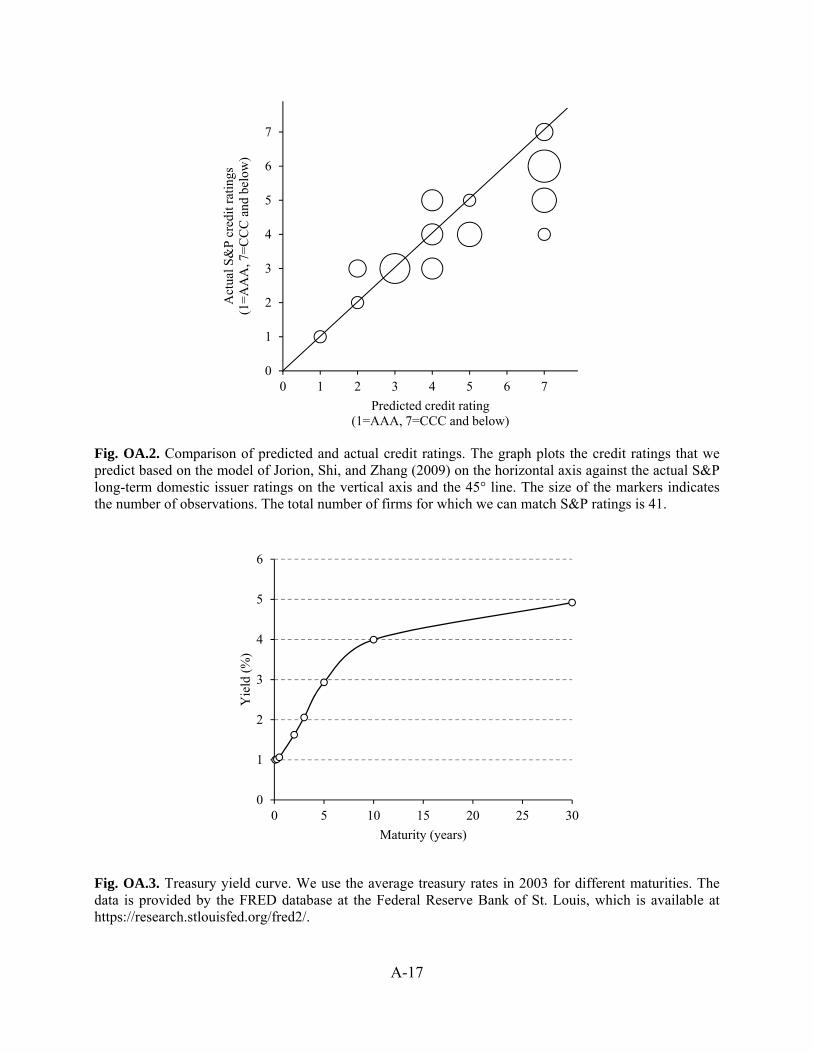
As a robustness check, Fig. OA.2 shows a bubble plot of the actual rating on the vertical

axis and the predicted rating on the horizontal axis for the 41 firms in our sample for which we

have both the actual S&P long-term domestic issuer rating and the predicted ratings. The

numbers on the axes represent ratings in ascending order with CCC and below being 7 and AAA

being 1. The Spearman rank order correlation is 0.995, indicating almost perfect prediction.

In order to compute the credit spread we use the average of the five- and ten-year spreads

as shown in Table OA.2. We add the credit spread that matches a firm’s predicted credit rating to

the Treasury rate from Fig. OA.3 corresponding to the firm’s typical project life using linear

interpolation. We take the average life of a typical project of each firm from their responses to the

survey (Question 3).

A-3

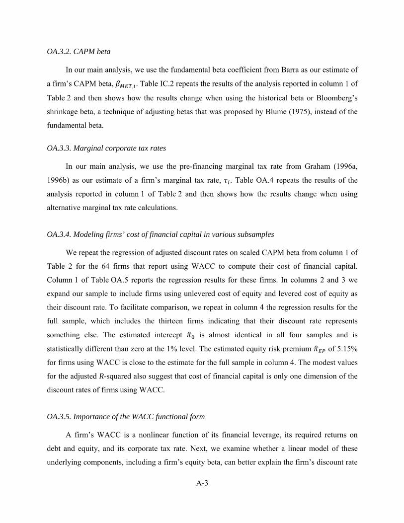
OA.3.2. CAPM beta

In our main analysis, we use the fundamental beta coefficient from Barra as our estimate of

a firm’s CAPM beta, , . Table IC.2 repeats the results of the analysis reported in column 1 of

Table 2 and then shows how the results change when using the historical beta or Bloomberg’s

shrinkage beta, a technique of adjusting betas that was proposed by Blume (1975), instead of the

fundamental beta.

OA.3.3. Marginal corporate tax rates

In our main analysis, we use the pre-financing marginal tax rate from Graham (1996a,

1996b) as our estimate of a firm’s marginal tax rate, . Table OA.4 repeats the results of the

analysis reported in column 1 of Table 2 and then shows how the results change when using

alternative marginal tax rate calculations.

OA.3.4. Modeling firms’ cost of financial capital in various subsamples

We repeat the regression of adjusted discount rates on scaled CAPM beta from column 1 of

Table 2 for the 64 firms that report using WACC to compute their cost of financial capital.

Column 1 of Table OA.5 reports the regression results for these firms. In columns 2 and 3 we

expand our sample to include firms using unlevered cost of equity and levered cost of equity as

their discount rate. To facilitate comparison, we repeat in column 4 the regression results for the

full sample, which includes the thirteen firms indicating that their discount rate represents

something else. The estimated intercept is almost identical in all four samples and is

statistically different than zero at the 1% level. The estimated equity risk premium of 5.15%

for firms using WACC is close to the estimate for the full sample in column 4. The modest values

for the adjusted R-squared also suggest that cost of financial capital is only one dimension of the

discount rates of firms using WACC.

OA.3.5. Importance of the WACC functional form

A firm’s WACC is a nonlinear function of its financial leverage, its required returns on

debt and equity, and its corporate tax rate. Next, we examine whether a linear model of these

underlying components, including a firm’s equity beta, can better explain the firm’s discount rate

A-4

than does WACC itself. In this analysis, we regress stated discount rates, , of the 64 firms that

use WACC as their discount rate directly on the components of WACC. The results are reported

in Table OA.6. If firms use the CAPM along with WACC to determine their discount rates, then

the discount rates should be correlated with firms’ CAPM betas. To test for this relationship, we

examine CAPM beta as the single explanatory variable. The coefficient estimate on the CAPM

beta, reported in column 1, is positive; however, the coefficient is insignificant and the R-squared

is very low, indicating that beta alone cannot explain discount rates. This finding is consistent

with Poterba and Summers (1995).

The univariate regression does not account for the other components of cost of financial

capital. Therefore, we regress self-reported discount rates on the debt-to-asset ratio, firms’

before-tax cost of debt, marginal tax rate, and two components of the CAPM, the risk-free rate

and the Barra fundamental beta. As reported in column 2, none of the five WACC components is

significantly related to firms’ discount rates, and the specification’s adjusted R-squared is

negative. The coefficient on CAPM beta is again positive and statistically insignificant. The cost

of debt is positively related with discount rates, however, its standard error is relatively high, and

the ratio debt-to-total capital is negatively related to discount rates.

If managers really use WACC, however, then a linear regression on these five components

is misspecified, because the variables should affect discount rates through the nonlinear WACC

formula. Therefore, to assess the importance of the WACC formula, we estimate the following

specification:

, , (OA.2)

where 

, , (OA.3)

and

, 1 , . (OA.4)

The term corresponds to the part of WACC that we deducted in Eq. (2) from the self-

reported discount rate to compute the adjusted discount rate. It combines all the terms that are not

directly related to the compensation for equity risk. If the model is correctly specified, then the

A-5

coefficient estimate provides an estimate of the equity risk premium and the coefficient

estimate should be one. The term is a constant, and is the error term.

As reported in column 3, both components of WACC are positively related to discount

rates. The estimated equity risk premium is 2.6% and is statistically significant at the 10% level.

The increase in adjusted R-squared from –0.015 in column 2 to 0.048 in column 3 supports the

view that the various components of WACC enter nonlinearly through the WACC formula.

However, as before, the cost of financial capital alone cannot explain much of the variation in

discount rates. In the final specification, equals 0.027 with a standard error of 0.227, so we

can clearly reject the hypothesis that equals one. The estimated equity risk premium is also

low when compared to the 3.83% value from Graham and Harvey (2005). These specification

tests indicate that there are variables missing from the model.1

The question arises: Is the adjusted R-squared of 4.8% in column 3 of Table OA.6 just

noise or are the discount rates firms use positively related to their systematic risk? To answer this

question we conduct the following Monte Carlo simulation. For each firm, we assign a debt-to-

equity ratio, a cost of debt, and a tax rate that are randomly drawn from the sample. Then we re-

estimate Eq. (OA.2) and compute the probability that we would observe an adjusted R-squared of

0.048. We find that there is only a 4.4% probability that, when assigning randomly the WACC

components other than beta, the adjusted R-squared would attain 0.048. Hence, our finding of a

positive relation between firms’ discount rates and systematic risk (i.e., , ) in the cross-

section is unlikely to be due to chance alone.

OA.3.6. Do firms use other models for their cost of equity capital? 

We also investigate whether the difference between firms’ discount rates and their costs of

financial capital comes from firms using other models instead of the CAPM to estimate their cost

of equity capital. While 73.5% of the respondents in Graham and Harvey’s (2001) survey use the

CAPM, 34.3% answer that they include some additional risk factors. Respondents to our survey

                                                            1 Another way to interpret the specification in column 3 of Table OA.6 is modeling the discount rate as

a linear function of WACC: , i.e., , . It follows from the estimates reported in column 3 of Table OA.6 that 0.0264 and 0.0269 ,

i.e., that the equity risk premium is .

.0.9814, which is almost 100%. The data thus clearly

rejects the model that firms’ discount rates are a simple linear function of WACC; there appear to be omitted variables that are correlated with the residuals.

A-6

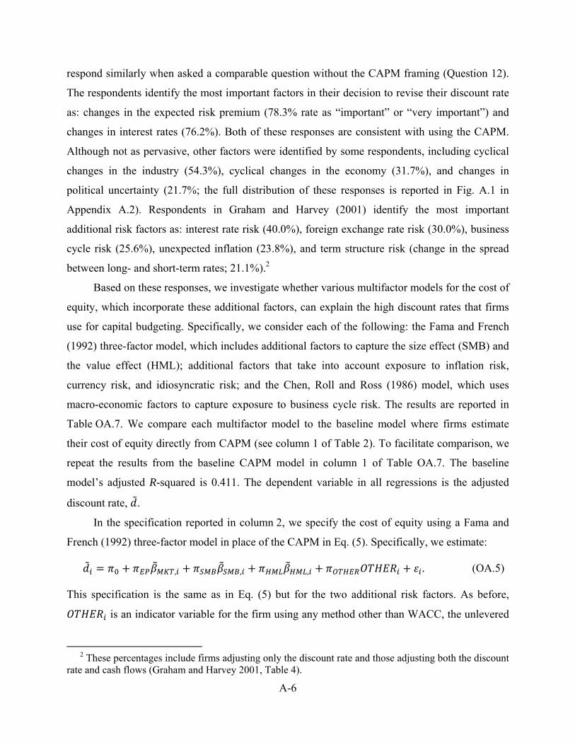
respond similarly when asked a comparable question without the CAPM framing (Question 12).

The respondents identify the most important factors in their decision to revise their discount rate

as: changes in the expected risk premium (78.3% rate as “important” or “very important”) and

changes in interest rates (76.2%). Both of these responses are consistent with using the CAPM.

Although not as pervasive, other factors were identified by some respondents, including cyclical

changes in the industry (54.3%), cyclical changes in the economy (31.7%), and changes in

political uncertainty (21.7%; the full distribution of these responses is reported in Fig. A.1 in

Appendix A.2). Respondents in Graham and Harvey (2001) identify the most important

additional risk factors as: interest rate risk (40.0%), foreign exchange rate risk (30.0%), business

cycle risk (25.6%), unexpected inflation (23.8%), and term structure risk (change in the spread

between long- and short-term rates; 21.1%).2

Based on these responses, we investigate whether various multifactor models for the cost of

equity, which incorporate these additional factors, can explain the high discount rates that firms

use for capital budgeting. Specifically, we consider each of the following: the Fama and French

(1992) three-factor model, which includes additional factors to capture the size effect (SMB) and

the value effect (HML); additional factors that take into account exposure to inflation risk,

currency risk, and idiosyncratic risk; and the Chen, Roll and Ross (1986) model, which uses

macro-economic factors to capture exposure to business cycle risk. The results are reported in

Table OA.7. We compare each multifactor model to the baseline model where firms estimate

their cost of equity directly from CAPM (see column 1 of Table 2). To facilitate comparison, we

repeat the results from the baseline CAPM model in column 1 of Table OA.7. The baseline

model’s adjusted R-squared is 0.411. The dependent variable in all regressions is the adjusted

discount rate, .

In the specification reported in column 2, we specify the cost of equity using a Fama and

French (1992) three-factor model in place of the CAPM in Eq. (5). Specifically, we estimate:

, , , . (OA.5)

This specification is the same as in Eq. (5) but for the two additional risk factors. As before,

is an indicator variable for the firm using any method other than WACC, the unlevered

                                                            2 These percentages include firms adjusting only the discount rate and those adjusting both the discount

rate and cash flows (Graham and Harvey 2001, Table 4).

A-7

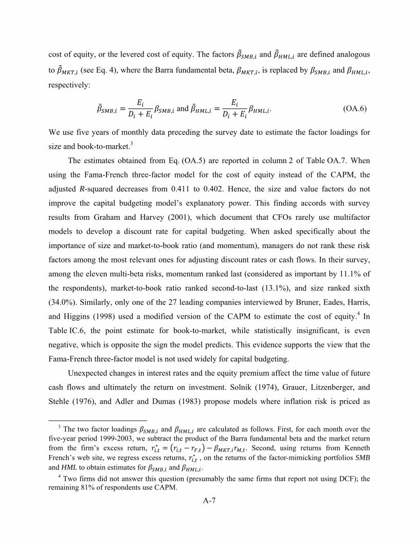
cost of equity, or the levered cost of equity. The factors , and , are defined analogous

to , (see Eq. 4), where the Barra fundamental beta, , , is replaced by , and , ,

respectively:

, , and , , . (OA.6)

We use five years of monthly data preceding the survey date to estimate the factor loadings for

size and book-to-market.3

The estimates obtained from Eq. (OA.5) are reported in column 2 of Table OA.7. When

using the Fama-French three-factor model for the cost of equity instead of the CAPM, the

adjusted R-squared decreases from 0.411 to 0.402. Hence, the size and value factors do not

improve the capital budgeting model’s explanatory power. This finding accords with survey

results from Graham and Harvey (2001), which document that CFOs rarely use multifactor

models to develop a discount rate for capital budgeting. When asked specifically about the

importance of size and market-to-book ratio (and momentum), managers do not rank these risk

factors among the most relevant ones for adjusting discount rates or cash flows. In their survey,

among the eleven multi-beta risks, momentum ranked last (considered as important by 11.1% of

the respondents), market-to-book ratio ranked second-to-last (13.1%), and size ranked sixth

(34.0%). Similarly, only one of the 27 leading companies interviewed by Bruner, Eades, Harris,

and Higgins (1998) used a modified version of the CAPM to estimate the cost of equity.4 In

Table IC.6, the point estimate for book-to-market, while statistically insignificant, is even

negative, which is opposite the sign the model predicts. This evidence supports the view that the

Fama-French three-factor model is not used widely for capital budgeting.

Unexpected changes in interest rates and the equity premium affect the time value of future

cash flows and ultimately the return on investment. Solnik (1974), Grauer, Litzenberger, and

Stehle (1976), and Adler and Dumas (1983) propose models where inflation risk is priced as

                                                            3 The two factor loadings , and , are calculated as follows. First, for each month over the

five-year period 1999-2003, we subtract the product of the Barra fundamental beta and the market return from the firm’s excess return, ,

∗, , , , . Second, using returns from Kenneth

French’s web site, we regress excess returns, ,∗ , on the returns of the factor-mimicking portfolios SMB

and HML to obtain estimates for , and , . 4 Two firms did not answer this question (presumably the same firms that report not using DCF); the

remaining 81% of respondents use CAPM.

A-8

investors use part of their portfolio to hedge against domestic inflation risk.5 Chen, Roll, and

Ross (1986), de Santis and Gérard (1997), Vassalou (2000), and Moerman and van Dijk (2010)

find evidence that inflation risk is priced.

In analysis reported in column 3, we test whether inflation risk can explain the variation in

the discount rates that firms use for capital budgeting. Similar to the factor loadings for SMB and

HML, we compute the inflation beta by regressing the excess returns ,∗ on changes in the

inflation index. Discount rates that are positively related to inflation provide a hedge against

inflation risk. Therefore, we would expect a negative coefficient for the inflation risk premium.

The estimated coefficient for inflation risk, however, is positive and statistically significant at the

5% level, suggesting that the inflation beta, which is computed from past realized changes in

inflation, may be proxying for other (omitted) economy wide risk factors.6 Although the

coefficient is statistically significant, the adjusted R-squared increases only slightly from the

baseline 0.411 to 0.431.

Next, we consider exchange rate risk. A number of empirical studies document that

exchange rate risk is priced in major stock markets (e.g., Dumas and Solnik, 1995; de Santis and

Gérard, 1998; Doukas, Hall, and Lang, 1999). Others, such as Chen, Roll, and Ross (1986) find

mixed evidence, while Jorion (1991) concludes that exchange rate risk is not priced.

In analysis reported in column 4, we test whether exchange rate risk can explain the

variation in the discount rates that firms use for capital budgeting. To assess a firm’s exchange

rate risk sensitivity, we first regress the excess returns ,∗ on changes in the U.S. dollar-Yen

exchange rate.7 We then include this sensitivity in our model for firms’ adjusted discount rate.

We find that currency risk is not priced in capital budgeting, as the coefficient in column 4 is

small and not statistically different from zero. This result may not be surprising as the majority of

empirical studies, including Jorion (1990), Choi and Prasad (1995), and Griffin and Stulz (2001),

                                                            5 In these models, the price of inflation risk is negative such that assets whose returns are high in times

of high inflation earn lower expected returns. Ferson and Harvey (1991) argue that the premium for inflation risk could be positive if inflation has negative real effects and firms differ in their exposure to changes in inflation.

6 Indeed, the estimated inflation risk premium is much smaller and statistically insignificant if we also control for the firms’ sensitivity to industrial production, , , discussed below.

7 Not only is it difficult to determine which currency pair is most relevant for the cash flows of our sample firms, but we also do not have information on the degree of hedging and thus a firm’s net currency risk exposure. Firms that hedge their currency risk will exhibit a lower exchange rate sensitivity.

A-9

find only weak evidence of currency exposure for U.S. firms, even when analyzing

multinationals. Firms hedge against exchange rate risk by matching exchange rate risk on the

asset and liability side and by using financial derivatives, which will mitigate their overall

exchange rate exposure. Bartram (2008) provides a clinical study of a large nonfinancial

multinational firm and shows that its residual foreign exchange rate exposure is small.

Next, we test whether macroeconomic risk factors have a significant impact on firms’

discount rates. Indeed, the CFOs surveyed by Graham and Harvey (2001) stress the importance

of interest rate risk and business cycle risk for capital budgeting. Chen, Roll, and Ross (1986)

estimate a multifactor asset pricing model that includes exposure to the following factors:

industrial production growth, unexpected inflation, changes in expected inflation, the slope of the

yield curve, and the credit risk premium. We analyze their set of macroeconomic factors and, as

before, compute the sensitivities by regressing five years of monthly excess returns on monthly

data for each of these five macroeconomic variables.

The results are reported in column 5 of Table OA.7. While the risk premium, , for the

firms’ sensitivity to the growth rate of industrial production, , , is negative and statistically

significant in this specification, this result is not robust to including other covariates.8 When we

replace in column 5 the unanticipated inflation beta, , , with the inflation beta from column 3,

, , its coefficient becomes insignificant ( 0.106, with a standard error of 0.300).

This suggests that the inflation beta computed from past realized changes in inflation proxies for

the business cycle, and the significance of the inflation beta disappears once we include a macro

variable for economic growth.

In sum, in line with results from previous surveys, we find that firms in our sample do not

use multifactor models to calculate their cost of equity for the purpose of capital budgeting.

OA.3.7. Variation in discount rates across additional firm characteristics

In Table 4 of the article, we report average discount rates for various subsamples of firms.

We use each of various variables constructed from survey answers or archival sources to

construct two subsamples and then tabulate means and standard errors for each subsample and p-

values from difference-in-means t-tests between the two subsamples. In Table OA.8 we include                                                             

8 If we include the firms’ sensitivity to the growth rate of industrial production, , , in the model reported below in Table OA.13 in the Online Appendix OA.4.5, the coefficient is half the magnitude and not statistically significant.

A-10

the same statistics describing discount rates for subsamples formed using additional variables

from our analyses.

Firms with higher CAPM betas use higher discount rates (p < 0.05), which is consistent

with firms using CAPM to calculate their cost of financial capital. Furthermore, the average

discount rates are significantly different for subsamples formed based on the current ratio (p <

0.05), number of business segments (p < 0.10), earnings surprises (p < 0.10), and market share (p

< 0.01). These unconditional differences, however, do not control for systematic risk. In further

analysis, we find that for all of these subsamples, with the exception of those formed based on the

current ratio, the subsample with higher average discount rate also has a higher CAPM beta.

Controlling for systematic risk likely explains why these other variables are not significant in our

regression analysis (see Tables 7 and 8 in the article). The current ratio has cash (and cash

equivalents) in its numerator, which we find to be an important determinant of firms’ discount

rates.

OA.4. Additional robustness tests

OA.4.1. Including the one outlier

In the main text, we exclude one outlier firm that reports using a discount rate of 40, which

is one-third greater than the next highest reported discount rate of 30%. In our regression model

of firms’ discount rates, the outlier observation has a studentized residual of 5.9 and is the only

observation whose studentized residual exceeds the critical value of 2 (Ruppert 2004). The

article’s conclusions are robust to addressing this outlier in other ways. Table OA.9 reports key

specifications from the article after including the outlier in the sample and using either OLS (in

Panel A) or robust regression analysis (in Panel B). Robust regression analysis, which we

implement using Stata’s rreg command, computes iteratively reweighted least squares, where

higher weights are given to well behaved observations and observations with Cook's distance

greater than 1 are excluded from the analysis.

The coefficient estimates and significance levels are similar in both sets of results, with the

exception of the variable measuring operational constraints, . Whereas is insignificant

when using OLS, its coefficient estimates are more than twice as large and statistically significant

at the 5% level when using robust regression. Significance levels also exhibit modest variations

A-11

for self-reported financial constraints, FINC; Altman’s Z-score, ; and the estimated equity

risk premium, .

OA.4.2. Restricting the sample to firms that use WACC

As reported in Table OA.10, we find similar results when restricting the sample to firms

that say they use WACC. The results for this subsample provide an even stronger case against

financial constraints as the negative coefficient on the self-reported financial constraints

indicator, , is statistically significant at the 5% level and the coefficient on Altman’s Z-

score, , increases from 0.0284 to 0.0360. The coefficient estimate on cash holdings, ,

is not statistically significant in combination with only the CAPM beta but is again statistically

significant at the 1% level in the combined model in the last column of Table OA.10. The

coefficient estimate on idiosyncratic risk, , is significant at only the 10% level in

combination with only the CAPM beta but is again statistically significant at the 5% level in the

combined model.

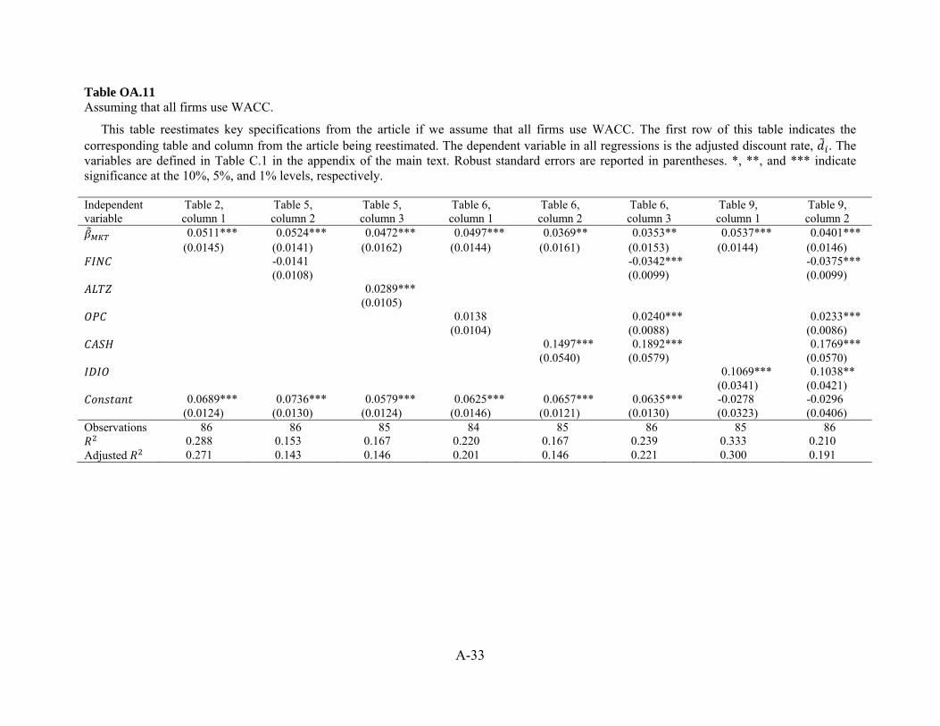
OA.4.3. Assuming that all firms use WACC

To further corroborate our main findings, we repeat the analysis again, this time treating all

firms as if they use WACC regardless of what they respond in the survey. Under this assumption

adjusted discount rates, , and scaled CAPM beta, , , are calculated as in Eqs. (3) and (4)

for all firms. The results are reported in Table OA.11. The results are again broadly similar, and

the significance levels for all of the coefficient estimates are the same as in the analysis in the

main text that accounts for the cost of capital method firms report to use. There are slight

variations in the coefficient estimates. For example, in all specifications shown in Table OA.11,

the estimate for the equity risk premium is lower than in our analysis in the main text; and in

most specifications, the constant term is higher.

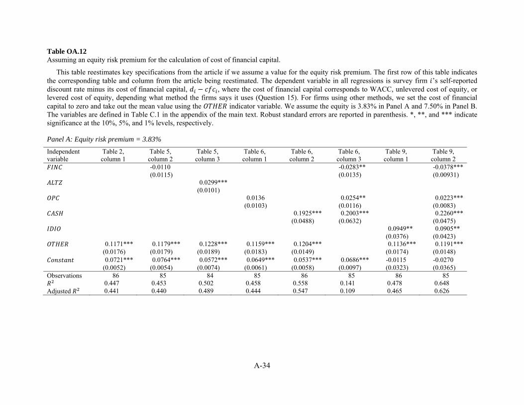
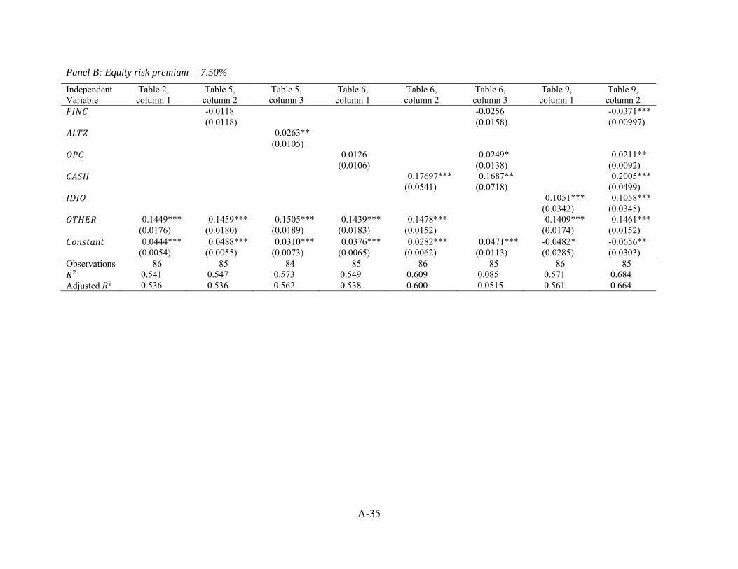
OA.4.4. Assuming an equity risk premium

Next, instead of inferring the equity risk premium from the data, we assume an equity risk

premium. We consider two potential values for the equity risk premium: (i) 3.83%, which CFOs

report to use at the time of our survey (Graham and Harvey, 2005), and (ii) 7.50%, which is a

plausible upper bound (Fama and French, 2002). In Table OA.12, we repeat the analysis for the

A-12

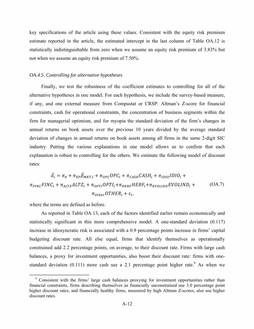
key specifications of the article using these values. Consistent with the equity risk premium

estimate reported in the article, the estimated intercept in the last column of Table OA.12 is

statistically indistinguishable from zero when we assume an equity risk premium of 3.83% but

not when we assume an equity risk premium of 7.50%.

OA.4.5. Controlling for alternative hypotheses

Finally, we test the robustness of the coefficient estimates to controlling for all of the

alternative hypotheses in one model. For each hypothesis, we include the survey-based measure,

if any, and one external measure from Compustat or CRSP: Altman’s Z-score for financial

constraints, cash for operational constraints, the concentration of business segments within the

firm for managerial optimism, and for myopia the standard deviation of the firm’s changes in

annual returns on book assets over the previous 10 years divided by the average standard

deviation of changes in annual returns on book assets among all firms in the same 2-digit SIC

industry. Putting the various explanations in one model allows us to confirm that each

explanation is robust to controlling for the others. We estimate the following model of discount

rates:

,

,

(OA.7)

where the terms are defined as before. 

As reported in Table OA.13, each of the factors identified earlier remain economically and

statistically significant in this more comprehensive model. A one-standard deviation (0.117)

increase in idiosyncratic risk is associated with a 0.9 percentage points increase in firms’ capital

budgeting discount rate. All else equal, firms that identify themselves as operationally

constrained add 2.2 percentage points, on average, to their discount rate. Firms with large cash

balances, a proxy for investment opportunities, also boost their discount rate: firms with one-

standard deviation (0.111) more cash use a 2.1 percentage point higher rate.9 As when we

                                                            9 Consistent with the firms’ large cash balances proxying for investment opportunities rather than

financial constraints, firms describing themselves as financially unconstrained use 3.0 percentage point higher discount rates, and financially healthy firms, measured by high Altman Z-scores, also use higher discount rates.

A-13

examine the hypotheses individually, neither of the managerial biases appear to play an important

role in determining the firm’s discount rate. Controlling for these factors also does not alter our

conclusions about the other hypotheses, as the estimates pertaining to idiosyncratic risk,

operational constraints, and financial constraints are similar to those of the combined model

reported in column 2 of Table 9.

References

Adler, M., and Dumas, B. 1983. International portfolio choice and corporation finance: a synthesis. Journal of Finance 38, 925–984.

Bartram, S., 2008. What lies beneath: Foreign exchange rate exposure, hedging and cash flows. Journal of Banking and Finance 32, 1508–1521.

Bierman, H. Jr., 1993. Capital budgeting in 1992: A survey. Financial Management 22, 24.

Blume, M., 1975. Betas and their regression tendencies. Journal of Finance 30, 785–795.

Brigham, E., 1975. Hurdle rates for screening capital expenditure proposals. Financial Management 4, 17–26.

Bruner, R., Eades, K., Harris, R., Higgins, R., 1998. Best practices in estimating the cost of capital: Survey and synthesis. Financial Practice and Education 8 (Spring/Summer), 13v28.

Chen, N.-F., Roll, R., Ross, S., 1986. Economic forces and the stock market. Journal of Business 59, 383–403.

Choi, J., Prasad, A., 1995. Exchange risk sensitivity and its determinants: A firm and industry analysis of U.S. multinationals. Financial Management 24, 77–88.

Doukas, J., Hall, P., Lang, L., 1999. The pricing of currency risk in Japan. Journal of Banking and Finance 23, 1–20.

Dumas, B., Solnik, B., 1995. The world of foreign exchange risk. Journal of Finance 50, 445–479.

de Santis, G., Gerard, B. 1997. International asset pricing and portfolio diversification with time-varying risk. Journal of Finance 52, 1881–1912.

de Santis, G., Gerard, B., 1998. How big is the premium for currency risk? Journal of Financial Economics 49, 375–412.

Fama, E., French, K. 1992. The cross-section of expected stock returns. Journal of Finance 47, 427–465.

Ferson, W., Harvey, C., 1991. The variation of economic risk premiums. Journal of Political Economy 99, 385–415.

Fama, E., French, K. 2002. The equity premium. Journal of Finance 57, 637–659.

Fremgen, J., 1973. Capital budgeting practices: A survey. Management Accounting 54, 19–25.

A-14

Gitman, L., Forrester, J. Jr., 1977. A survey of capital budgeting techniques used by major U.S. firms. Financial Management 6, 66–71.

Gitman, L., Mercurio, V., 1982. Cost of capital techniques used by major U.S. firms: Survey and analysis of Fortune’s 1000. Financial Management 11, 21–29.

Gitman, L., Vandenberg, P., 2000. Cost of capital techniques used by major U.S. firms: 1997 vs. 1980. Financial Practice and Education 10, 53–68.

Graham, J., 1996a. Debt and marginal tax rate. Journal of Financial Economics 41, 41–73.

Graham, J., 1996b. Proxies for the corporate marginal tax rate. Journal of Financial Economics 42, 187–221.

Graham, J., Harvey, C., 2001. The theory and practice of corporate finance: Evidence from the field. Journal of Financial Economics 60, 187–243.

Graham, J., Harvey, C., 2005. The long-run equity risk premium. Finance Research Letters 2, 185–194.

Graham, J., Harvey, C., 2009. Duke/CFO Magazine Global Business Outlook, U.S. topline tables, released September 16, 2009, www.cfosurvey.org/pastresults.htm.

Graham, J., Harvey, C., 2011a. Duke/CFO Magazine Global Business Outlook, U.S. topline tables, released March 9, 2011, www.cfosurvey.org/pastresults.htm.

Graham, J., Harvey, C., 2011b. Duke/CFO Magazine Global Business Outlook, U.S. topline tables, released September 13, 2011, www.cfosurvey.org/pastresults.htm.

Graham, J., Harvey, C., 2012. Duke/CFO Magazine Global Business Outlook, U.S. topline tables, released June 6, 2012, www.cfosurvey.org/pastresults.htm.

Grauer, F., Litzenberger, R., Stehle, R., 1976. Sharing rules and equilibrium in an international capital market under uncertainty. Journal of Financial Economics 3, 233–256.

Griffin, J., Stulz, R., 2001. International competition and exchange rate shocks: A cross-country industry analysis of stock returns. Review of Financial Studies 14, 215–241.

Istvan, D., 1961. The economic evaluation of capital expenditures. Journal of Business 34, 45–51.

Jacobs, M., Shivdasani, A., 2012. Do you know your cost of capital? Harvard Business Review 7/8, 118–124.

Jorion, P., 1990. The exchange-rate exposure of U.S. multinationals. Journal of Business 63, 331–345.

Jorion, P., 1991. The pricing of exchange rate risk in the stock market. Journal of Financial and Quantitative Analysis 26, 363–376.

Jorion, P., Charles S., Zhang, W., 2009. Tightening credit standards: The role of accounting quality. Review of Accounting Studies 14, 123–160.

Kim, S., Farragher, E., 1981. Current capital budgeting practices. Management Accounting 61, 26–30.

A-15

Klammer, Thomas P., 1972, Empirical evidence of the adoption of sophisticated capital budgeting techniques, Journal of Business 45(3), 387-397.

Klammer, T., Walker, M., 1984. The continuing increase in the use of sophisticated capital budgeting techniques. California Management Review 27, 137–148.

Mao, J., 1970. Survey of capital budgeting: Theory and practice. Journal of Finance 25, 349–360.

Moerman, G., van Dijk, M., 2010. Inflation risk and international asset returns. Journal of Banking and Finance 34, 840–855.

Moore, J., Reichert, A. 1983. An analysis of the financial management techniques currently employed by large U.S. corporations. Journal of Business, Finance, and Accounting 10, 623–645.

Petry, G., 1975. Effective use of capital budgeting tools. Business Horizons (October), 57–65.

Petty, W., Bowlin, O., 1976. The financial manager and quantitative decision models. Financial Management 5, 32–41.

Petty, W., Scott, D. Jr., Bird, M., 1975. The capital expenditure decision-making process of large corporations. Engineering Economist 20, 159–172.

Poterba, J., Summers, L., 1995. A CEO survey of U.S. companies’ time horizon and hurdle rates. Sloan Management Review (Fall), 43–53.

Ruppert, D., 2004. Statistics and Finance: An Introduction. Springer, New York.

Schall, L., Sundem, G., Geijsbeek, W. Jr., 1978. Survey and analysis of capital budgeting methods. Journal of Finance 38, 281–287.

Solnik, B., 1974. An equilibrium model of the international capital market. Journal of Economic Theory 8, 500–524.

Trahan, E., Gitman, L., 1995. Bridging the theory-practice gap in corporate finance: A survey of chief financial officers. Quarterly Review of Economics and Finance 35, 73–87.

Vassalou, M., 2000. Exchange rate and foreign inflation risk premiums in global equity returns. Journal of International Money and Finance 19, 433–470.

A-16

Figure OA.1. Adoption of DCF methods, WACC, CAPM, and company-wide discount rates over time. Surveys on capital budgeting practices of U.S. firms are listed in chronological order by survey date below the horizontal time axis. The plot summarizes their findings regarding the percentage of firms that: (i) use discounted cash flow (DCF) methods, including net present value (NPV), adjusted present value (APV), internal rate of return (IRR), and the profitability index (PI); (ii) use the weighted average cost of capital (WACC) to discount cash flows; (iii) use the Capital Asset Pricing Model (CAPM) to compute the cost of equity; and (iv) use a company-wide discount rate.

A-17

Fig. OA.2. Comparison of predicted and actual credit ratings. The graph plots the credit ratings that we predict based on the model of Jorion, Shi, and Zhang (2009) on the horizontal axis against the actual S&P long-term domestic issuer ratings on the vertical axis and the 45° line. The size of the markers indicates the number of observations. The total number of firms for which we can match S&P ratings is 41.

Fig. OA.3. Treasury yield curve. We use the average treasury rates in 2003 for different maturities. The data is provided by the FRED database at the Federal Reserve Bank of St. Louis, which is available at https://research.stlouisfed.org/fred2/.

0

1

2

3

4

5

6

7

0 1 2 3 4 5 6 7

Act

ual S

&P

cre

dit r

atin

gs

(1=

AA

A, 7

=C

CC

and

bel

ow)

Predicted credit rating(1=AAA, 7=CCC and below)

0

1

2

3

4

5

6

0 5 10 15 20 25 30

Yie

ld (

%)

Maturity (years)

A-18

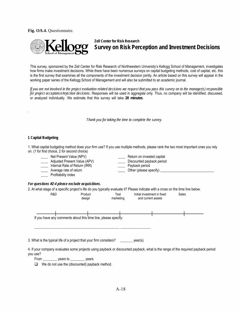
Fig. OA.4. Questionnaire.

Zell Center for Risk Research

Survey on Risk Perception and Investment Decisions This survey, sponsored by the Zell Center for Risk Research of Northwestern University’s Kellogg School of Management, investigates how firms make investment decisions. While there have been numerous surveys on capital budgeting methods, cost of capital, etc. this is the first survey that examines all the components of the investment decision jointly. An article based on this survey will appear in the working paper series of the Kellogg School of Management and will also be submitted to an academic journal. If you are not involved in the project evaluation related decisions we request that you pass this survey on to the manager(s) responsible for project acceptance/rejection decisions. Responses will be used in aggregate only. Thus, no company will be identified, discussed, or analyzed individually. We estimate that this survey will take 20 minutes.

.

Thank you for taking the time to complete the survey. I. Capital Budgeting 1. What capital budgeting method does your firm use? If you use multiple methods, please rank the two most important ones you rely on. (1 for first choice, 2 for second choice)

____ Net Present Value (NPV) ____ Return on invested capital ____ Adjusted Present Value (APV) ____ Discounted payback period ____ Internal Rate of Return (IRR) ____ Payback period ____ Average rate of return ____ Other (please specify) ______________________________ ____ Profitability index

For questions #2-4 please exclude acquisitions.

2. At what stage of a specific project’s life do you typically evaluate it? Please indicate with a cross on the time line below.

R&D Product Test Initial investment in fixed Sales design marketing and current assets

If you have any comments about this time line, please specify: ________________________________________________ _________________ 3. What is the typical life of a project that your firm considers? _______ year(s) 4. If your company evaluates some projects using payback or discounted payback, what is the range of the required payback period you use?

From ________ years to ________ years

We do not use the (discounted) payback method.

A-19

II. Hurdle Rates/Risk 5. In evaluating projects, does your company use

hurdle rates/target rates/discount rates that incorporate the expected future inflation (i.e. nominal hurdle rates) hurdle rates/target rates/discount rates that do not include inflation expectations (i.e. real hurdle rates)

6. In nominal terms (i.e. incorporating the expected future inflation), what is the hurdle your company has used for a typical project during the last two years?

_______ % 7. Does your hurdle rate depend on the expected life of a project?

Yes No

If your answer is “Yes”, do you use a higher rate for

longer life projects or shorter life projects 8. If you use multiple hurdle rates, what is the lowest and highest hurdle rate you use?

Lowest hurdle rate _______ %

Highest hurdle rate _______ % 9. In evaluating strategic projects (where accepting a given project today may enable the firm to make additional future investments), do you

use a lower hurdle rate than you would for a similar non- strategic project value the potential projects in the future separately and add their value to the strategic project evaluate strategic projects in the same manner as non- strategic projects If your company has multiple divisions/business segments please answer #10, otherwise skip to #11

10. If you calculate the hurdle rate for a division/business segment, do you

Never Always -2 -1 0 1 2

use the company-wide hurdle rate

use the hurdle rate of firms that are in the same industry as the division in question (proxy firms)

adjust the industry hurdle rate of proxy firms for tax rate, cost of debt, capital structure, etc., differences between your firm and proxy firms

11. How often did you change the hurdle rate(s) in the past three years?

We have not changed the hurdle rate(s) during the past three years Once More than once 12. If you were to change your hurdle rate(s), how important would the following factors be?

Not important Very important -2 -1 0 1 2 Interest rate changes Cyclical changes in the economy

Cyclical changes in the industry(ies) you operate in

Changes in political uncertainty Changes in the expected risk premium Changes in the corporate tax rates

13. How important are the following factors in determining the hurdle rate you use?

Not important Very important -2 -1 0 1 2

Whether it is a short-lived or long-lived project

Whether it is a strategic or non-strategic investment

Whether it is a replacement project or a new investment

Whether it is a revenue expansion or a cost reduction project

Whether it is a domestic project or a foreign project

Whether the project in question requires significantly more funds than the typical project your firm takes

14. How important are the following risk factors in determining the hurdle rate?

Not important Very important -2 -1 0 1 2

Market risk of a project, defined as the sensitivity of the project returns to economic conditions

Project risk that is unique to the firm and unrelated to the state of the economy

15. The hurdle rate you use represents the firm’s

weighted average cost of capital cost of levered equity capital cost of unlevered equity Other (please specify) ______________________________ ____________________ ____________________________

A-20

 

III. Cash Flows 16. In evaluating projects, the cash flows you use are calculated as

earnings before interest and after taxes (EBIAT) + depreciation earnings before interest and after taxes (EBIAT) + depreciation – capital expenditures – net change in working capital earnings earnings + depreciation earnings + depreciation – capital expenditures – net change in working capital Other (please specify) ______________________________ ____________________________ ____________________ 17. In estimating future sales, cost of goods sold, etc., do you include the expected inflation rate in your cash flow projections?

Yes No 18. In valuing projects, do you incorporate into the cash flows the money you spent before the period when you make the accept/reject decision?

Yes No 19. If a new product will cause a decline in the sales of an existing product (erosion, cannibalization), do you subtract the erosion from the estimated sales figures of the new project?

Yes Yes, but only if competitors are likely to introduce a product similar to the new product Yes, but only if the competitors are unlikely to introduce a similar product No 20. To what extent do these statements agree with your company’s views?

Strongly disagree Strongly agree -2 -1 0 1 2

We need a higher hurdle rate to account for optimism in cash flow forecasts

There are some good projects we cannot take due to limited access to capital markets

We cannot take all profitable projects due to limited resources in the form of limited qualified management and manpower

We invest more in projects in years when the firm has more operating cash flows

21. How do you incorporate risk into project evaluation?

Not important Very important -2 -1 0 1 2

Increase the hurdle rate Decrease the estimated cash flows

If your firm does not have foreign investments, please skip questions #22 and #23.

22. For foreign investments do you

use higher hurdle rates than for similar domestic projects use more conservative cash flow estimates than for similar domestic projects Both Neither Other ___________________________________________ 23. For foreign investments do you

translate the foreign currency cash flows of the project into dollars by using forward rates and use the domestic (dollar based) hurdle rate discount foreign currency cash flows using the hurdle rate calculated from data of the foreign country in question Other __________________________________________ IV. Capital Structure 24. In deciding how to finance projects in your firm, in what order would you use the following sources of capital to fund profitable projects? (1 for first choice, 2 if the first choice does not raise sufficient amount of capital, 3 if the first two choices do not meet the project’s total financing needs, 4, 5, etc.)

____ Internally available excess cash balances ____ Short-term debt ____ Long-term debt ____ Operating profits ____ Equity issues ____ Other (please specify) _________________________ ___________________________________________ 25. The advantage of debt for your firm is that

Strongly disagree Strongly agree -2 -1 0 1 2

interest payments are tax-deductible it forces the firm to be more efficient

debt is a cheaper source of funds even if the interest payments were not tax-deductible

it provides substantial financial flexibility

A-21

 

26. The advantage of equity is that Strongly disagree Strongly agree -2 -1 0 1 2

it increases the firm’s flexibility it reduces costs of financial distress

it does not obligate the firm to make payments to shareholders

27. What factors determine the optimal debt/equity mix of your firm?

Strongly disagree Strongly agree -2 -1 0 1 2

We borrow to the extent that the marginal interest tax shield becomes zero

We do not borrow at all so the firm will not operate in financially distressed situations

We borrow until the tax advantage becomes equal to the financial distress disadvantages of debt

We borrow below our debt capacity so that if we run into very valuable projects in the future we can tap into the unused debt capacity

28. We would borrow more if

Strongly disagree Strongly agree -2 -1 0 1 2

we had more taxable income we had more tangible assets we were in a higher tax rate

V. Other 29. Compared with the current capital structure your company’s intention for the next three years is to

keep your debt/equity ratio the same increase your debt/equity ratio, i.e. move towards more debt than now decrease your debt/equity ratio, i.e. move towards more equity than now 30. Company characteristics

Industry Retail and Wholesale Mining, Construction Manufacturing Communication/Media Technology (Software, Biotech, etc.) Services Utility Other (please specify) _____________________________

Company characteristics (continued)

Sales $100 million $100-499 million $500-999 million $1-5 billion > $5 billion 31. Does your firm have multiple product lines?

Yes No 32. Company ownership

Public Private

If your answer is “Public”, what is the firm’s current price-to-earnings ratio? ________ 33. What is the interest rate on senior long-term debt? ________ 34. What is the approximate equity stake of senior management in the firm?

_______ % Don’t know

Our last two questions are about you and the ticker/name of your company. The ticker symbol will only be used to gather additional, publicly available data from databases such as Compustat. All responses will be used in aggregate only. No company will be identified, discussed or analyzed individually. 35. Information about the person completing the form

Age Time in job Education ≤ 39 < 4 years Undergraduate 40-49 5-9 years MBA 50-59 ≥ 10 years non MBA masters ≥ 60 > masters degree

What year did you graduate from your last school? ___________ 36. Ticker symbol or company name

________________________________ ____________________

Thank you for completing the survey!

A-22

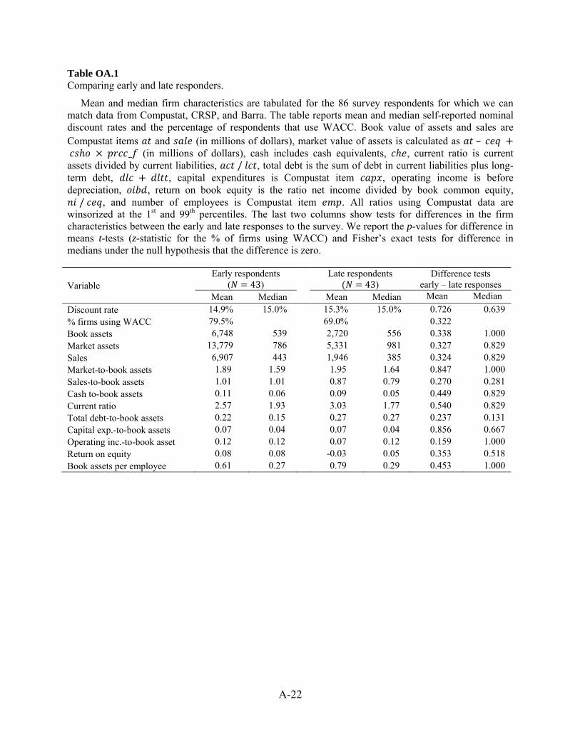
Table OA.1 Comparing early and late responders.

Mean and median firm characteristics are tabulated for the 86 survey respondents for which we can match data from Compustat, CRSP, and Barra. The table reports mean and median self-reported nominal discount rates and the percentage of respondents that use WACC. Book value of assets and sales are Compustat items and (in millions of dollars), market value of assets is calculated as – _ (in millions of dollars), cash includes cash equivalents, , current ratio is current assets divided by current liabilities, / , total debt is the sum of debt in current liabilities plus long-term debt, , capital expenditures is Compustat item , operating income is before depreciation, , return on book equity is the ratio net income divided by book common equity, / , and number of employees is Compustat item . All ratios using Compustat data are

winsorized at the 1st and 99th percentiles. The last two columns show tests for differences in the firm characteristics between the early and late responses to the survey. We report the p-values for difference in means t-tests (z-statistic for the % of firms using WACC) and Fisher’s exact tests for difference in medians under the null hypothesis that the difference is zero.

Variable Early respondents

( 43) Late respondents

43)Difference tests

early – late responses Mean Median Mean Median Mean Median

Discount rate 14.9% 15.0% 15.3% 15.0% 0.726 0.639% firms using WACC 79.5% 69.0% 0.322 Book assets 6,748 539 2,720 556 0.338 1.000Market assets 13,779 786 5,331 981 0.327 0.829Sales 6,907 443 1,946 385 0.324 0.829Market-to-book assets 1.89 1.59 1.95 1.64 0.847 1.000Sales-to-book assets 1.01 1.01 0.87 0.79 0.270 0.281Cash to-book assets 0.11 0.06 0.09 0.05 0.449 0.829Current ratio 2.57 1.93 3.03 1.77 0.540 0.829Total debt-to-book assets 0.22 0.15 0.27 0.27 0.237 0.131Capital exp.-to-book assets 0.07 0.04 0.07 0.04 0.856 0.667Operating inc.-to-book asset 0.12 0.12 0.07 0.12 0.159 1.000Return on equity 0.08 0.08 -0.03 0.05 0.353 0.518Book assets per employee 0.61 0.27 0.79 0.29 0.453 1.000

 

A-23

Table OA.2 Credit spreads.

This table summarizes the spreads over Treasury rates by rating category. For the rating categories AAA through BB, we report the average of the five-year and ten-year spreads of corporate bonds. The individual bond indices of different rating categories are from Bloomberg and include liquid traded bonds with weekly data starting 02/13/1996 and only bonds which have a minimum outstanding of USD 100 million. For the rating category B, since the S&P data ends in 2002, the spread between AAA and B in 2002 is calculated. Using the 2003 yield of AAA rated bonds and the 2002 spread for B bonds over AAA bonds, the yields of B rated bonds are calculated to be 6.09%. For bond ratings which are CCC and below, the Bank of America Merrill Lynch US High Yield CCC or Below Option-Adjusted Spread (obtained from the Global Financial Database) is used to compute the average spread of 12.96% for these bonds in 2003.

Credit rating Bloomberg ticker Average credit

spread Five-year spread Ten-year spread

AAA SPWC3A5 SPWC3A10 0.75% AA SPWC2A5 SPWC2A10 0.87% A SPWCA5 SPWCA10 1.13% BBB SPWC3B5 SPWC3B10 2.43% BB SPWC2B5 SPWC2B10 4.36% B SPWCB5 SPWCB10 6.09% CCC and below 12.96%

A-24

Table OA.3 Using alternative beta estimates.

We repeat the regression in column 1 of Table 2 using different definitions of the CAPM beta, . The dependent variable in all specifications is the transformed discount rate . Column 1 is added for comparisons and repeats the results from Table 2 using the fundamental beta from Barra. In column 2 we use monthly data to estimate beta from a regression of firm’s returns on the returns of the S&P 500 over the past five years. Column 3 reports the firm’s Bloomberg shrinkage beta that puts a weight of 0.667 on the historical beta and 0.333 on one.

Independent varialble

(1) (2) (3) Fundamental beta Historical beta Shrinkage beta

0.0587*** 0.0305*** 0.0522*** (0.0129) (0.0106) (0.0151)

0.134*** 0.112*** 0.129*** (0.0199) (0.0192) (0.0208)

0.0550*** 0.0771*** 0.0599*** (0.0105) (0.0092) (0.0121)

Observations 86 86 86 0.424 0.361 0.395

Adjusted 0.411 0.346 0.381

Table OA.4 Using alternative estimates of marginal corporate tax rates.

We repeat the regression in column 1 of Table 2 using different estimates for firms’ marginal corporate tax rate, . The dependent variable in all specifications is the transformed discount rate . Column 1 is added for comparisons and repeats the results from Table 2 using the before-debt tax rate of Graham (1996a, 1996b). In column 2 we set tax rates to 0% for all firms, in (3) we use 34%, and in (4) the average tax rate of the firm (total tax paid divided by pre-tax income; Compustat items txt / pi).

Independent variable

(1) (2) (3) (4) Graham 0% Rate 34% rate Average rate

0.0587*** 0.0702*** 0.0563*** 0.0650*** (0.0129) (0.0149) (0.0129) (0.0146)

0.134*** 0.149*** 0.130*** 0.142*** (0.0199) (0.0211) (0.0198) (0.0208)

0.0550*** 0.0398*** 0.0589*** 0.0475*** (0.0105) (0.0127) (0.0103) (0.0121)

Observations 86 86 86 86 0.424 0.439 0.419 0.428

Adjusted 0.411 0.426 0.405 0.414

 

A-25

Table OA.5 Modeling discount rates using the cost of financial capital.

This table summarizes results from linear regressions that model firms’ discount rates as their cost of financial capital:

, .

The sample in column 1 includes the 64 firms that use WACC as their discount rate. In column 2, we add the six firms using unlevered cost of equity as their cost of financial capital. Column 3 further adds three firms that indicate to use the levered cost of equity as their cost of financial capital. In column 4, we include the 13 firms that use other methods to compute their cost of financial capital. The variables are defined in Table C.1 in the appendix of the main text. Robust standard errors are reported in parentheses. *, **, and *** indicate significance at the 10%, 5%, and 1% levels, respectively.

Independent variable

(1) (2) (3) (4)

WACC WACC

+ unlevered

WACC + unlevered

+ levered All firms

0.0515*** 0.0572*** 0.0587*** 0.0587*** (0.0133) (0.0136) (0.0128) (0.0129)

0.1340*** (0.0199)

0.0558*** 0.0556*** 0.0550*** 0.0550*** (0.0113) (0.0108) (0.0105) (0.0105)

Observations 64 70 73 86 0.211 0.219 0.239 0.424

Adjusted 0.199 0.208 0.228 0.411

 

A-26

Table OA.6 Relating discount rates to the components of the weighted average cost of capital.

This table summarizes results from linear regressions of the firms’ discount rate on the components of WACC. The dependent variable in all the regressions is the firms’ discount rate from the survey, . The sample is restricted to the 64 firms that respond to use WACC to compute their cost of financial capital. In column 1, the independent variable is the firms’ fundamental beta provided by Barra, , .

, ,

In column 2, the independent variables are the various components of WACC:

, / , , ,

In column 3, we run the following regression:

, ,

, , and , 1 , .

, is a scaled version of , and is a coefficient that is expected to be one if the model is correctly specified. The other variables are defined in Table C.1 in the appendix of the main text. Robust standard errors are reported in parentheses. *, **, and *** indicate significance at the 10%, 5%, and 1% levels, respectively.

Independent variable

(1) (2) (3)

Beta WACC

components Cost of debt and

cost of equity 0.0133 0.0142

(0.0131) (0.0128) ⁄ -0.0322

(0.0243) 0.0564

(0.1016) 0.0225

(0.0350) 0.0092

(0.5402) 0.0264*

(0.0143) 0.0269

(0.2270) 0.1267*** 0.1210*** 0.1190***

(0.0128) (0.0239) (0.0186) Observations 64 64 64

0.028 0.065 0.079 Adjusted 0.013 -0.015 0.048

A-27

Table OA.7 Modeling discount rates using multifactor models.

This table summarizes the results of linear regressions that include different sets of systematic risk factors in our baseline model. The dependent variable in all regressions is the adjusted discount rate, . Column 1 repeats the results of the baseline model in column 1 of Table 2.

In column 2, we specify the cost of equity as a Fama-French three-factor model:

, , , ,

where , , and , , are defined analogous to , , where Barra beta

is replaced by the factor loadings and that we estimate using five years of monthly data over the period 1999-2003. For firm , we subtract each month the product of the firm’s Barra beta and the market return, , , , from its excess return, ,

∗, , ; then we regress these excess returns ,

∗ on the returns of the factor-mimicking portfolios and to get the estimates of , and , .

is a constant and is an idiosyncratic error. The other variables are defined in Table C.1 in the appendix of the main text.

Column 3 shows the results for a 2-factor model for , with the equity beta and inflation beta:

, , ,

where , , , and the inflation beta , is computed as follows: For firm , we regress

the excess returns from before, ,∗ , on the monthly inflation rates, log log ,

where is the seasonally adjusted Consumer Price Index (all urban consumers, U.S. city average, all items; CUSR000SA0 series) from the Bureau of Labor Statistics. The coefficient on the inflation return is the firm’s inflation beta , .

In column 4, we have a 2-factor model with the equity beta and a currency:

, , ,

where , , and the currency beta , is computed in the same manner as the inflation beta,

regressing the excess returns ,∗ on the monthly returns of the USD-Yen index instead. The coefficient on

the USD-Yen return is the currency beta , .

Model (5) includes the macroeconomic factors from Chen, Roll, and Ross (1986):

, ,

, , , , ,

where , , , , , , , , , , , , and ,

, . Analogous to the inflation beta, , , above, we regress the monthly excess return ,∗ on

, , , , and , respectively, over the previous five years to get the estimates of , ,

, , , , , , and , . log log is the monthly growth rate in industrial production, where is the Industrial Production Index (INDPRO series) in month from the FRED database at the Federal Reserve Bank of St. Louis, which measures real output of facilities located in the U.S. in manufacturing, mining, electric, and gas utilities. E | 1 is the unanticipated inflation, where is the inflation rate based on the seasonally adjusted Consumer Price Index as above. E | 1 , E | 1 , where , is the one-month Treasury bill rate from CRSP (file crsp.mcti, variable t30ret) and , . E | E |1 is the change in expected inflation. is the unanticipated change in the term structure, defined as the

A-28

difference between the 20-year (20-Year Treasury Constant Maturity Rate; series GS20) minus the 1-year (1-Year Treasury Constant Maturity Rate; series DGS1) Treasury yield from the FRED database at the Federal Reserve Bank of St. Louis. UPR is the unanticipated change in the risk premium, defined as the Baa-Aaa yield spread (Moody’s Seasoned Baa Corporate Bond Yield minus Moody’s Seasoned Aaa Corporate Bond Yield) from the FRED database at the Federal Reserve Bank of St. Louis.

Robust standard errors are reported in parentheses. *, **, and *** indicate significance at the 10%, 5%, and 1% levels, respectively.

Independent variable

(1) (2) (3) (4) (5) CAPM Fama-French Inflation Currency Chen-Roll-Ross

0.0587*** 0.0525*** 0.0506*** 0.0572*** 0.0572*** (0.0129) (0.0146) (0.0138) (0.0134) (0.0133)

0.0040 (0.0080)

-0.0060 (0.0077)

0.4220** (0.2060)

-0.0081 (0.0184)

  -0.0028**   (0.0012)

  -0.0002   (0.0007)

  0.0000   (0.0003)

  0.0020   (0.0018)

  -0.0007   (0.0006)

0.1340*** 0.1290*** 0.1300*** 0.1330*** 0.1350*** (0.0199) (0.0212) (0.0202) (0.0204) (0.0207)

0.0550*** 0.0604*** 0.0591*** 0.0565*** 0.0543*** (0.0105) (0.0125) (0.0110) (0.0113) (0.0112)

Observations 86 86 86 86 86 0.424 0.431 0.452 0.426 0.476

Adjusted 0.411 0.402 0.431 0.405 0.429

A-29

Table OA.8 Variation in discount rates across additional firm characteristics.

The table reports average discount rates (and standard errors in parentheses) for various subsamples of firms. In each row, the variable in the first column is used to define above median and below median subsamples, whose statistics are reported in the second and third columns. The last column reports p-values for difference in mean t-tests between the two subsamples. The variables are , the CAPM beta, and measures of cost of financial constraints, managerial optimism, and managerial myopia. The measures of financial constraint are: , the current ratio; ⁄ , financial leverage; and , the Kaplan-Zingales index. The measures of managerial optimism are: , the firm’s number of business segments; , the firm’s concentration of business segments; and , the market value of the firm’s assets. The measures of managerial myopia are: , the average absolute percent difference between earnings per share forecasts and actual earnings; , the observed sensitivity of stock prices to earnings news in the industry; , sale concentration of firms in the industry; and

, the firm’s market share. The variables are defined in Table C.1.

Variable used to form subsamples

Above median Below medianp-Value

of difference 0.161 0.141 0.047

(0.007) (0.006) 0.161 0.140 0.035

(0.008) (0.006) ⁄ 0.145 0.156 0.285

(0.007) (0.007) 0.148 0.153 0.645

(0.006) (0.008) 0.148 0.159 0.073

(0.006) (0.007) 0.159 0.143 0.108

(0.007) (0.007) 0.144 0.158 0.163

(0.006) (0.008) 0.164 0.142 0.054

0.009) 0.006) 0.143 0.158 0.144

(0.007) (0.007) 0.145 0.156 0.298

(0.007) (0.007) 0.135 0.165 0.003

(0.006) (0.007)

A-30

Table OA.9 Including the one outlier.

This table reestimates key specifications from the article after including the outlier firm that is excluded from the article’s analytic sample. The outlier firm reports a discount rate of 40%, which it says represents its unlevered cost of equity. The first row of this table indicates the corresponding table and column from the article being reestimated. The dependent variable in all regressions is the adjusted discount rate, . We report the results using ordinary least squares (OLS) in Panel A and robust regression in Panel B, which is estimated using Stata’s rreg command. The variables are defined in Table C.1 in the appendix of the main text. Robust standard errors are reported in parenthesis. *, **, and *** indicate significance at the 10%, 5%, and 1% levels, respectively.

Panel A: OLS regressions

Independent variable

Table 2, column 1

Table 5, column 2

Table 5, column 3

Table 6, column 1

Table 6, column 2

Table 6, column 3

Table 9, column 1

Table 9, column 2

0.0693*** 0.0699*** 0.0621*** 0.0688*** 0.0510*** -0.0161 0.0706*** 0.0527*** (0.0167) (0.0163) (0.0173) (0.0171) (0.0164) (0.0183) (0.0168) (0.0161)

-0.0065 -0.0221 -0.0278** (0.0123) (0.0163) (0.0131)

0.0323*** (0.0107)

0.0064 0.0160 0.0122 (0.0117) (0.0145) (0.0127)

0.1829*** 0.2715*** 0.2042*** (0.0496) (0.0717) (0.0507)

0.112*** 0.1051** (0.0371) (0.0425)

  0.1394*** 0.1402*** 0.13980*** 0.138*** 0.1285*** 0.136*** 0.1276***   (0.0206) (0.0207) (0.0216) (0.0215) (0.0189) (0.0200) (0.0181)

0.0498*** 0.0519*** 0.0392*** 0.0468*** 0.0464*** 0.1027*** -0.0497 -0.0456 (0.0118) (0.0132) (0.0127) (0.0118) (0.0125) (0.0144) (0.0370) (0.0411) Observations 87 86 85 86 87 86 87 86

0.381 0.380 0.440 0.380 0.466 0.183 0.421 0.526 Adjusted 0.366 0.357 0.419 0.357 0.447 0.143 0.400 0.490

A-31

Panel B: Robust regressions

Independent Variable

Table 2, column 1

Table 5, column 2

Table 5, column 3

Table 6, column 1

Table 6, column 2

Table 6, column 3

Table 9, column 1

Table 9, column 2

0.0563*** 0.0567*** 0.0469*** 0.0553*** 0.0406*** 0.0359*** 0.0595*** 0.0419*** (0.0139) (0.0141) (0.0138) (0.0135) (0.0137) (0.0127) (0.0136) (0.0129)

-0.0142 -0.0320*** -0.0351*** (0.0105) (0.0100) (0.0101)

0.0304*** (0.0100)

0.0193* 0.0257*** 0.0245** (0.0099) (0.00937) (0.00942)

0.1824*** 0.2193*** 0.2013*** (0.0460) (0.0446) (0.0451)

0.0914** 0.0814** (0.0431) (0.0393)

  0.1237*** 0.1273*** 0.1299*** 0.1161*** 0.1177*** 0.115*** 0.1220*** 0.1179***   (0.0179) (0.0181) (0.0178) (0.0173) (0.0168) (0.0156) (0.0175) (0.0157)

0.0555*** 0.0600*** 0.0475*** 0.0470*** 0.0521*** 0.0506*** -0.0269 -0.0230 (0.0122) (0.0128) (0.0124) (0.0128) (0.0113) (0.0115) (0.0402) (0.0367) Observations 87 86 85 86 87 86 87 86

0.363 0.378 0.446 0.382 0.478 0.554 0.398 0.566 Adjusted 0.348 0.355 0.425 0.359 0.459 0.526 0.376 0.533  

   

A-32

Table OA.10 Restricting the sample to firms that use WACC.

This table reestimates key specifications from the article after restricting the sample to firms that say they use WACC. The first row of this table indicates the corresponding table and column from the article being reestimated. The dependent variable in all regressions is the adjusted discount rate, . The variables are defined in Table C.1 in the appendix of the main text. Robust standard errors are reported in parentheses. *, **, and *** indicate significance at the 10%, 5%, and 1% levels, respectively. 

Independent variable

Table 2, column 1

Table 5, column 2

Table 5, column 3

Table 6, column 1

Table 6, column 2

Table 6, column 3

Table 9, column 1

Table 8, column 2

0.0515*** 0.0517*** 0.0433*** 0.0516*** 0.0469*** 0.0421*** 0.0539*** 0.0457*** (0.0133) (0.0119) (0.0152) (0.0133) (0.0142) (0.0126) (0.0138) (0.0119)

-0.0250** -0.0391*** -0.0432*** (0.0105) (0.0098) (0.00996)

0.0360*** (0.0096)

0.0131 0.0222** 0.0226** (0.0100) (0.0089) (0.00854)

0.0650 0.1360** 0.143*** (0.0690) (0.0626) (0.0526)

0.0638* 0.0897** (0.0374) (0.0383)

0.0558*** 0.0649*** 0.0441*** 0.0490*** 0.0543*** 0.0552*** -0.0017 -0.0253 (0.0113) (0.0109) (0.0108) (0.0125) (0.0117) (0.0116) (0.0361) (0.0373) Observations 64 63 64 63 64 63 64 63

0.211 0.281 0.372 0.229 0.227 0.392 0.243 0.451 Adjusted 0.199 0.257 0.351 0.203 0.202 0.350 0.218 0.403

A-33

Table OA.11 Assuming that all firms use WACC.

This table reestimates key specifications from the article if we assume that all firms use WACC. The first row of this table indicates the corresponding table and column from the article being reestimated. The dependent variable in all regressions is the adjusted discount rate, . The variables are defined in Table C.1 in the appendix of the main text. Robust standard errors are reported in parentheses. *, **, and *** indicate significance at the 10%, 5%, and 1% levels, respectively.

Independent variable

Table 2, column 1

Table 5, column 2

Table 5, column 3

Table 6, column 1

Table 6, column 2

Table 6, column 3

Table 9, column 1

Table 9, column 2

0.0511*** 0.0524*** 0.0472*** 0.0497*** 0.0369** 0.0353** 0.0537*** 0.0401*** (0.0145) (0.0141) (0.0162) (0.0144) (0.0161) (0.0153) (0.0144) (0.0146)

-0.0141 -0.0342*** -0.0375*** (0.0108) (0.0099) (0.0099)

0.0289*** (0.0105)

0.0138 0.0240*** 0.0233*** (0.0104) (0.0088) (0.0086)

0.1497*** 0.1892*** 0.1769*** (0.0540) (0.0579) (0.0570)

0.1069*** 0.1038** (0.0341) (0.0421)

0.0689*** 0.0736*** 0.0579*** 0.0625*** 0.0657*** 0.0635*** -0.0278 -0.0296 (0.0124) (0.0130) (0.0124) (0.0146) (0.0121) (0.0130) (0.0323) (0.0406) Observations 86 86 85 84 85 86 85 86

0.288 0.153 0.167 0.220 0.167 0.239 0.333 0.210 Adjusted 0.271 0.143 0.146 0.201 0.146 0.221 0.300 0.191  

   

A-34

Table OA.12 Assuming an equity risk premium for the calculation of cost of financial capital.

This table reestimates key specifications from the article if we assume a value for the equity risk premium. The first row of this table indicates the corresponding table and column from the article being reestimated. The dependent variable in all regressions is survey firm ’s self-reported discount rate minus its cost of financial capital, , where the cost of financial capital corresponds to WACC, unlevered cost of equity, or levered cost of equity, depending what method the firms says it uses (Question 15). For firms using other methods, we set the cost of financial capital to zero and take out the mean value using the indicator variable. We assume the equity is 3.83% in Panel A and 7.50% in Panel B. The variables are defined in Table C.1 in the appendix of the main text. Robust standard errors are reported in parenthesis. *, **, and *** indicate significance at the 10%, 5%, and 1% levels, respectively.

Panel A: Equity risk premium = 3.83%

Independent variable

Table 2, column 1

Table 5, column 2

Table 5, column 3

Table 6, column 1

Table 6, column 2

Table 6, column 3

Table 9, column 1

Table 9, column 2

-0.0110 -0.0283** -0.0378*** (0.0115) (0.0135) (0.00931)

0.0299*** (0.0101)

0.0136 0.0254** 0.0223*** (0.0103) (0.0116) (0.0083)

0.1925*** 0.2003*** 0.2260*** (0.0488) (0.0632) (0.0475)

0.0949** 0.0905** (0.0376) (0.0423)

  0.1171*** 0.1179*** 0.1228*** 0.1159*** 0.1204*** 0.1136*** 0.1191***   (0.0176) (0.0179) (0.0189) (0.0183) (0.0149) (0.0174) (0.0148)

0.0721*** 0.0764*** 0.0572*** 0.0649*** 0.0537*** 0.0686*** -0.0115 -0.0270 (0.0052) (0.0054) (0.0074) (0.0061) (0.0058) (0.0097) (0.0323) (0.0365) Observations 86 85 84 85 86 85 86 85

0.447 0.453 0.502 0.458 0.558 0.141 0.478 0.648 Adjusted 0.441 0.440 0.489 0.444 0.547 0.109 0.465 0.626

A-35

Panel B: Equity risk premium = 7.50%

Independent Variable

Table 2, column 1

Table 5, column 2

Table 5, column 3

Table 6, column 1

Table 6, column 2

Table 6, column 3

Table 9, column 1

Table 9, column 2

-0.0118 -0.0256 -0.0371*** (0.0118) (0.0158) (0.00997)

0.0263** (0.0105)

0.0126 0.0249* 0.0211** (0.0106) (0.0138) (0.0092)

0.17697*** 0.1687** 0.2005*** (0.0541) (0.0718) (0.0499)

0.1051*** 0.1058*** (0.0342) (0.0345)

  0.1449*** 0.1459*** 0.1505*** 0.1439*** 0.1478*** 0.1409*** 0.1461***   (0.0176) (0.0180) (0.0189) (0.0183) (0.0152) (0.0174) (0.0152)

0.0444*** 0.0488*** 0.0310*** 0.0376*** 0.0282*** 0.0471*** -0.0482* -0.0656** (0.0054) (0.0055) (0.0073) (0.0065) (0.0062) (0.0113) (0.0285) (0.0303) Observations 86 85 84 85 86 85 86 85

0.541 0.547 0.573 0.549 0.609 0.085 0.571 0.684 Adjusted 0.536 0.536 0.562 0.538 0.600 0.0515 0.561 0.664  

36

Table OA.13 Controlling for alternative hypotheses.

This table contains the results of a linear regression that includes measures of idiosyncratic risk, operational constraints, financial constraints, and managerial biases in our baseline model. We report results from the following specification:

,,

The variables are defined in Table C.1 in the appendix of the main text. Robust standard errors are reported in parentheses. *, **, *** indicate significance at the 10%, 5%, and 1% levels, respectively.

Independent variable

(1)

0.0383*** (0.0131)

  0.0775*   (0.0456)

0.0227** (0.0094)

0.1794*** (0.0498)

-0.0285*** (0.0102)

0.0187** (0.0092)

-0.0115 (0.0087)

0.0042 (0.0220)

-0.0020 (0.0122)

0.1234*** (0.0196)

-0.0205 (0.0443)

Observations 81 0.624

Adjusted 0.570