저 시-비 리- 경 지 2.0 한민

는 아래 조건 르는 경 에 한하여 게

l 저 물 복제, 포, 전송, 전시, 공연 송할 수 습니다.

다 과 같 조건 라야 합니다:

l 하는, 저 물 나 포 경 , 저 물에 적 된 허락조건 명확하게 나타내어야 합니다.

l 저 터 허가를 면 러한 조건들 적 되지 않습니다.

저 에 른 리는 내 에 하여 향 지 않습니다.

것 허락규약(Legal Code) 해하 쉽게 약한 것 니다.

Disclaimer

저 시. 하는 원저 를 시하여야 합니다.

비 리. 하는 저 물 리 목적 할 수 없습니다.

경 지. 하는 저 물 개 , 형 또는 가공할 수 없습니다.

공학박사학위논문

Monitoring of off-grid

renewable energy systems and

a load oriented model for energy

production and consumption

독립 신재생 전력망의 에너지

모니터링 및 부하 고려 모델 개발

2017년 8월

서울대학교 대학원

기계항공공학부

이 장 엽

i

Abstract

Demand for renewable energy sources has increased rapidly

due to global warming. Since 1990, the renewable energy

consumption ratio has increased among developed countries and

the OECD average reached over 10% in 2015. Even in

developing countries, an off-grid renewable power system has

been implemented in rural areas to provide electricity. However,

the power generation characteristics of renewable energy

sources are so random that power outages occur frequently.

In this research, an off-grid monitoring platform was

developed and applied to an off-grid renewable energy system

to overcome the instability of a renewable power system in

rural areas. Our monitoring platform contains a customized

real-time operating system with low-cost hardware for task

management. The monitoring platform was capable of

bidirectionally transmitting a data set via short message service

or the internet. The transmitted data set was uploaded to a

cloud system so that the off-grid system could be monitored

with any platform.

The energy consumption of manufacturing systems and

ii

renewable energy systems were modeled, and the operating

conditions were simulated. The simulation results provided 1)

the design guide for an off-grid system, 2) the failure rate with

various scales of off-grid systems, and 3) the calculation

method of operation times. Furthermore, the modeling method

could be applied to various types of electric load conditions.

Finally, an off-grid test bed was installed with our

developed monitoring platform and four case studies were

conducted: 1) a three dimensional printer, 2) a turning machine,

3) a band saw, and 4) a vaccine carrier, to verify the stability of

the off-grid energy system with manufacturing processes.

Comparison with previous research was also conducted, and the

proposed simulation method provided a smaller scale of off-

grid systems with stable operation.

Key words: renewable energy, energy consumption, modeling,

monitoring, off-grid

Student Number: 2012-20692

iii

Table of Contents

1 INTRODUCTION............................................................................. １

1.1 OVERVIEW ......................................................................................... １

1.2 STABILITY ISSUES IN RENEWABLE ENERGY SYSTEMS......................... ７

1.3 STABILITY ISSUES AND MANUFACTURING PROCESSES ....................... ９

2 RENEWABLE ENERGY PRODUCTION MODEL............................ １２

2.1 PV ENERGY PRODUCTION................................................................１２

2.1.1 Mathematical models and patterns of energy production .１２

2.2 WIND ENERGY PRODUCTION ............................................................１９

2.2.1 Mathematical models and patterns of energy production .１９

2.3 BATTERY MODEL ............................................................................２３

2.4 COMBINING MODELS FOR A RENEWABLE ENERGY PLANT .................２８

2.5 OPERATION TIME CALCULATIONS ...................................................２９

2.6 CONCLUSIONS ................................................................................３１

3 MANUFACTURING ENERGY CONSUMPTION MODEL................ ３２

3.1 OVERVIEW ......................................................................................３２

3.2 THEORETICAL BACKGROUNDS ON MANUFACTURING ENERGY

CONSUMPTION ......................................................................................３５

3.2.1 Cutting process energy consumption model ......................３８

3.2.2 Feed drive friction-based energy consumption model.....４２

3.3 STANDARDIZED ENERGY CONSUMPTION MEASUREMENT PROCEDURE . ４

３

3.3.1 Assumptions and experimental design ...............................４３

3.3.2 Data measurement and analysis procedure .......................４６

3.4 RESULTS ........................................................................................５１

3.5 ENERGY CONSUMPTION SIMULATOR................................................５７

3.5.1 Overview ...............................................................................５７

3.5.2 Simulation procedure and results........................................５９

3.6 MACHINE LEARNING-BASED ENERGY CONSUMPTION MODELING .....６８

3.6.1 Overview ...............................................................................６８

3.6.2 Physical model-based neural network design ..................６８

3.6.3 Backpropagation algorithm ..................................................７１

3.6.4 Results...................................................................................７１

iv

3.7 SUMMARY.......................................................................................７５

4 ENERGY MODEL FOR RENEWABLE ENERGY AND

MANUFACTURING PROCESSES .................................................... ７６

4.1 OVERVIEW ......................................................................................７７

4.2 ASSUMPTIONS OF MODELS..............................................................７９

4.3 GENERALIZED LOAD CONDITION......................................................８１

4.4 TEST BED FOR MODEL ....................................................................８４

4.5 MODELING RESULTS .......................................................................８８

4.5.1 Case study 1: 3D Printer .....................................................９１

4.5.2 Case study 2: Lathe ..........................................................１００

4.5.3 Case study 3: Band saw....................................................１０４

4.5.4 Case study 4: Vaccine carrier..........................................１０７

4.5.5 Comparison with other models.........................................１１０

4.6 SUMMARY....................................................................................１１４

5 CONCLUSIONS .........................................................................１１６

APPENDIX ...................................................................................１１８

MONITORING SYSTEM FOR A RENEWABLE ENERGY SYSTEM ................１１８

Issues in data transmission via telecommunication methods.......... １２４

Issues regarding bidirectional control.............................................. １２７

SUMMARY..........................................................................................１２７

OBJECTIVES.......................................................................................１２８

DEVELOPMENT OF AN OFF-GRID ENERGY MONITORING

PLATFORM..................................................................................１２９

OVERVIEW .........................................................................................１２９

REQUIREMENTS FOR AN OFF-GRID ENERGY MONITORING PLATFORM .１２９

OFF-GRID MONITORING PLATFORM ...................................................１３１

HARDWARE DESIGN FOR OFF-GRID MONITORING PLATFORM ..............１３２

Main processor............................................................................１３３

Sensors............................................................................................... １３３

Telecommunication device................................................................ １３６

SOFTWARE DESIGN FOR OFF-GRID MONITORING PLATFORM...............１３７

Customized real-time OS...........................................................１３７

Task management.............................................................................. １３８

Signal Processing .............................................................................. １３８

v

Low-speed data measurement..................................................... １３９

High-speed data measurement .................................................... １３９

DEVELOPMENT RESULTS ...................................................................１４０

DEVELOPMENT SUMMARY ..................................................................１４４

6 BIBLIOGRAPHY ........................................................................１４５

7 ABSTRACT IN KOREAN...........................................................１５４

vi

List of TablesTable 1. Verification parameters of the PV array...............................１８

Table 2. Composition and power losses of the feed drive system [54]４

２

Table 3. ANN design and training parameters ....................................７２

Table 4. Summary of simulation results...............................................７４

Table 5. Summation of various load conditions ...................................８３

Table 6. Solar panel specifications.......................................................８５

Table 7. MPPT solar charge controller specifications........................８７

Table 8. Wind turbine specifications ....................................................８７

Table 9. Battery specifications.............................................................８８

Table 10. Specifications of 3Dwox DP200, Shindoh Corp ..................９２

Table 11. Comparison result of HOMER and time-wise model.......１１３

Table 12. Previous research of off-grid renewable energy systems １２

１

Table 13. List of commercially available monitoring devices and SNU

monitoring system .......................................................................１２３

Table 14. Communication frequencies in Nepal ...............................１２４

Table 15. Detailed information of SMS cost .....................................１２５

vii

Table of FiguresFigure 1. Global mean estimates based on land and ocean data [1]..... ２

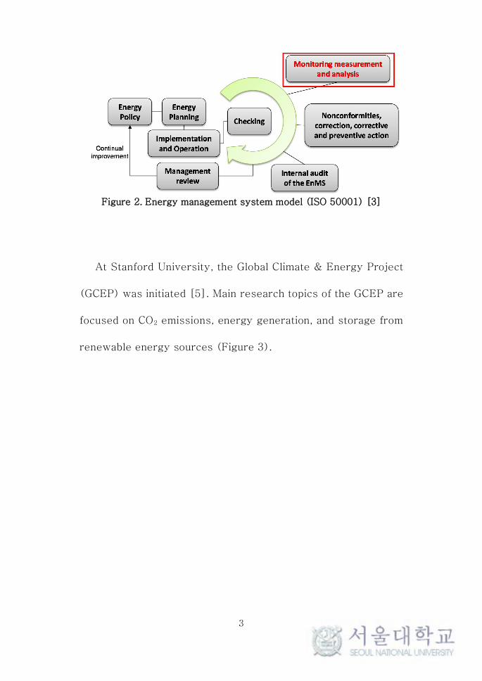
Figure 2. Energy management system model (ISO 50001) [3]............. ３

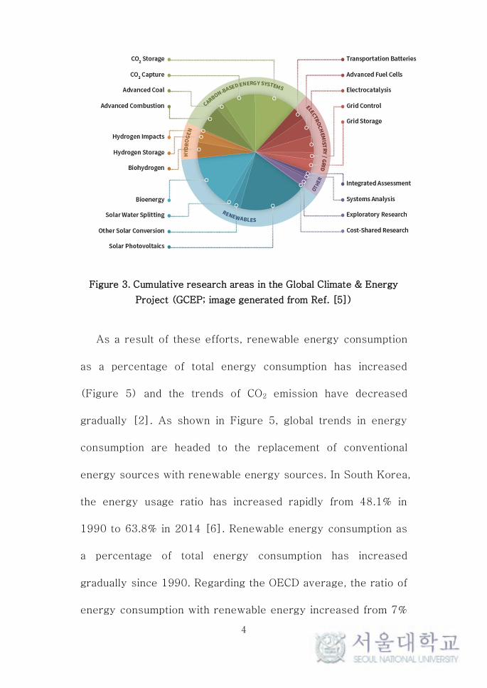
Figure 3. Cumulative research areas in the Global Climate & Energy

Project (GCEP; image generated from Ref. [5]) ............................. ４

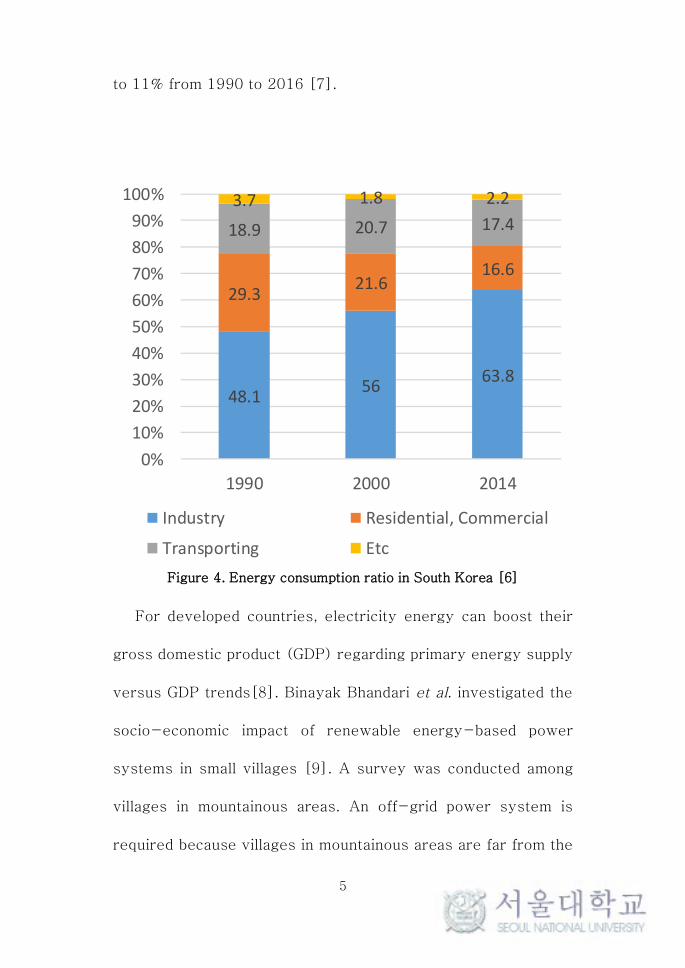
Figure 4. Energy consumption ratio in South Korea [6]........................ ５

Figure 5. Renewable energy consumption ratio [7]............................... ６

Figure 6. Typical pattern of renewable resources [11] ........................ ７

Figure 7. Hourly California renewable electricity production profile by

month (image from [12])................................................................... ８

Figure 8. Product costs for manufacturing ............................................. ９

Figure 9. Power demand for manufacturing (GS400)..........................１０

Figure 10. Failure example of manufacturing process with off-grid

energy system.................................................................................１１

Figure 11. Ideal single-diode photovoltaic (PV) cell model [32].......１３

Figure 12. Brief expression of an ideal single-diode PV cell model .１３

Figure 13. PV array model consists of multiple single-diode models１３

Figure 14. Typical I-V curve for an array of PVs...............................１６

Figure 15. Typical power curve for an array of PVs ..........................１６

Figure 16. Experimental result of PV model verification ...................１８

Figure 17. Typical power curve for a wind turbine.............................２１

Figure 18. Power output versus instantaneous wind speed of a 400-W

wind turbine ....................................................................................２２

Figure 19. Equivalent battery model [40] ...........................................２３

Figure 20. Relationship between temperature and discharge capacity

(provided by manufacturer)............................................................２５

Figure 21. Temperature vs. percent capacity surface........................２６

Figure 22. Equivalent battery model ....................................................２６

Figure 23. Schematics of the model for energy production and

consumption ....................................................................................２８

Figure 24. Operating times of the off-grid system (battery capacity =

240 Ah)............................................................................................３０

Figure 25. Operating times of the off-grid system (battery capacity =

320 Ah)............................................................................................３１

Figure 26. Research trends for machine tool energy consumption....３４

Figure 27. Cutting force diagram..........................................................３８

Figure 28. Merchant’s circle.................................................................３９

Figure 29. Trends of cutting speed versus cutting force [62]...........４０

Figure 30. Typical curve of the SEC model [48]................................４０

Figure 31. Detailed cutting power measurement procedure...............４７

Figure 32. Example of a power profile and power measurement

procedure ........................................................................................４８

Figure 33. Decomposition of additional electrical power requirement . ４

８

Figure 34. Block diagram of power trend acquisition setup...............５０

viii

Figure 35. Axis orientation of CNC lathe.............................................５１

Figure 36. Spindle power of the machine tools ...................................５２

Figure 37. The feed drive power of machine tools .............................５４

Figure 38. The cutting power of machine tools...................................５５

Figure 39. Flow chart describing the power profile simulation..........６１

Figure 40. Definition of the feed drive position vector.......................６１

Figure 41. Example of an actual power profile and a simulated power

profile ..............................................................................................６３

Figure 42. Simulated power profile of the machine tool peripherals .６６

Figure 43. Simulated power profile of the machine tools ...................６７

Figure 44. Block diagram of a two-layer artificial neural network (ANN)

[69]..................................................................................................６９

Figure 45. Results of performance index vs. number of iterations ....７３

Figure 46. Results of trained ANN .......................................................７４

Figure 47. Previous research on renewable energy and load conditions

.........................................................................................................７６

Figure 48. Flow chart of manufacturing-oriented renewable energy

simulation ........................................................................................７８

Figure 49. Schematics of generalized load condition..........................８１

Figure 50. Experimental results of various load conditions ...............８２

Figure 51. Off-grid renewable energy testbed in SNU.......................８４

Figure 52. Hardware block diagram for off-grid testbed in SNU ......８５

Figure 53. Power trends of direct measurement and modeled results . ８

９

Figure 54. Results of monitored voltage of battery bank (actual results)

.........................................................................................................９０

Figure 55. Results of monitored SOC of battery bank (actual results) . ９

１

Figure 56. Dimensions of the test specimen........................................９１

Figure 57. Operating position of manufacturing of target specimen..９２

Figure 58. Power trends of a three dimensional (3D) printer to fabricate

a target specimen ...........................................................................９３

Figure 59. SOC result with six PV arrays and two wind turbines......９３

Figure 60. SOC results with ten PV arrays and two wind turbines....９４

Figure 61. Surface of failure rate vs. scale of renewable energy system

(@ 1 × vwind) ....................................................................................９６

Figure 62. Surface of failure rate vs. scale of renewable energy system

(@ 3 × vwind) ....................................................................................９６

Figure 63. Surface of failure rate vs. scale of renewable energy system

(@ 5 × vwind) ....................................................................................９７

Figure 64. Verification of energy conservation in the redesigned off-

grid system......................................................................................９８

Figure 65. Failure rate of redesigned off-grid system with a

manufacturing process ...................................................................９９

Figure 66. SOC results of eight PV arrays, one wind turbine, and eight

batteries ..........................................................................................９９

ix

Figure 67. Results of battery bank voltage (actual data).................１００

Figure 68. Process procedure for case study: the lathe..................１０１

Figure 69. Surface of failure rate vs. scale of renewable energy system

(@ 1 × vwind) .................................................................................１０２

Figure 70. Surface of failure rate vs. scale of renewable energy system

(@ 3 × vwind) .................................................................................１０３

Figure 71. Power demand profile of the acrylic plate cutting process . １

０５

Figure 72. Simulation results of an off-grid renewable energy system

with a band saw ...........................................................................１０６

Figure 73. Power demand profile of a vaccine carrier with cooling on vs.

off..................................................................................................１０８

Figure 74. Simulation results of an off-grid renewable energy system

with a vaccine carrier..................................................................１０９

Figure 75. Monte Carlo analysis of a PV/wind/hydro system [80].１１１

Figure 76. Load condition example in HOMER Pro ..........................１１２

Figure 77. Optimal results obtained with HOMER Pro .....................１１３

Figure 78. Issues in an off-grid renewable energy system.............１１９

Figure 79. Communication coverage in Nepal ..................................１２５

Figure 80. Cost estimate of MMS per month....................................１２６

Figure 81. Cost estimate of SMS per month.....................................１２６

Figure 82. Schematic of a real-time online energy monitoring system １

２９

Figure 83. Schematic of an off-grid monitoring platform................１３１

Figure 84. Hardware schematics of the off-grid monitoring platform.. １

３２

Figure 85. Customized pyranometer .................................................１３４

Figure 86. Calibration results with the customized pyranometer....１３４

Figure 87. Output curve of the temperature sensor [103]..............１３５

Figure 88. Output curve of Hall effect-based current sensor [104] .１３

６

Figure 89. Database PC and backend data storage program in the

database layer..............................................................................１３６

Figure 90. Hardware schematic of the off-grid monitoring platform.１３

７

Figure 91. First test set up for data transmitting from Nepal to South

Korea ............................................................................................１４１

Figure 92. Results of SMS data transmission from Nepal................１４２

Figure 93. Images of sensor installation in Thingan, Nepal.............１４２

Figure 94. Monitoring device for off-grid power system in Thingan,

Nepal.............................................................................................１４３

Figure 95. Sensor data from Thingan on February 4–6th .................１４３

１

1 Introduction

1.1 Overview

Since the industrial revolution, the amount of CO2 emissions

worldwide has increased dramatically. Consequently, global

warming is now a problem, due to greenhouse gases generated

by fossil-fuel energy generation systems. Since 1970, the

global mean temperature has increased gradually and CO2

emissions have accelerated the effects of global warming [1].

As one effort to slow down global warming, the PBL

Netherlands Environmental Assessment Agency’s 2016 report

was published [2]. There are two major solutions to the global

warming problem: 1) energy consumption and 2) energy

generation.

２

Figure 1. Global mean estimates based on land and ocean data [1]

The International Organization for Standardization (ISO)

published the ISO 50001:2011 Energy management system for

managing energy consumption [3] (Figure 2). ISO also

published another standard, the ISO 14955 series for increasing

energy consumption efficiency in manufacturing industries [4].

-0.6

-0.4

-0.2

0

0.2

0.4

0.6

0.8

1

1.2

1880 1900 1920 1940 1960 1980 2000 2020

Tem

per

atu

re A

no

mal

y (

)

Annual Mean Lowess Smoothing

３

Figure 2. Energy management system model (ISO 50001) [3]

At Stanford University, the Global Climate & Energy Project

(GCEP) was initiated [5]. Main research topics of the GCEP are

focused on CO2 emissions, energy generation, and storage from

renewable energy sources (Figure 3).

４

Figure 3. Cumulative research areas in the Global Climate & Energy

Project (GCEP; image generated from Ref. [5])

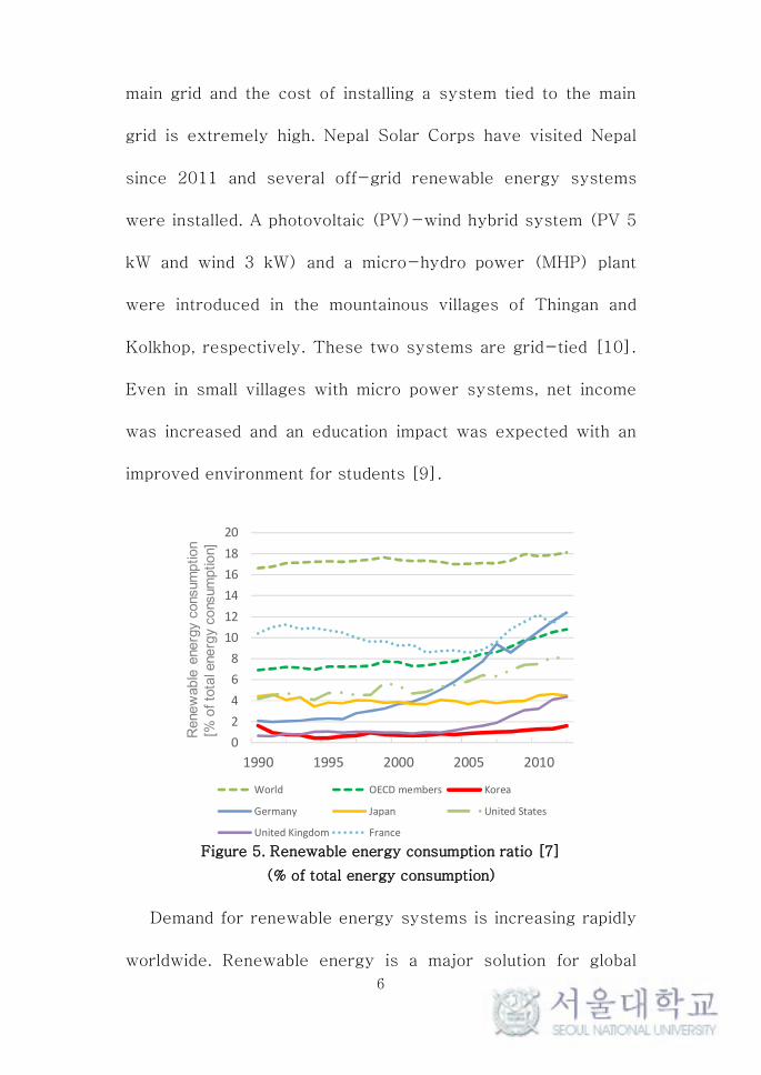
As a result of these efforts, renewable energy consumption

as a percentage of total energy consumption has increased

(Figure 5) and the trends of CO2 emission have decreased

gradually [2]. As shown in Figure 5, global trends in energy

consumption are headed to the replacement of conventional

energy sources with renewable energy sources. In South Korea,

the energy usage ratio has increased rapidly from 48.1% in

1990 to 63.8% in 2014 [6]. Renewable energy consumption as

a percentage of total energy consumption has increased

gradually since 1990. Regarding the OECD average, the ratio of

energy consumption with renewable energy increased from 7%

５

to 11% from 1990 to 2016 [7].

Figure 4. Energy consumption ratio in South Korea [6]

For developed countries, electricity energy can boost their

gross domestic product (GDP) regarding primary energy supply

versus GDP trends[8]. Binayak Bhandari et al. investigated the

socio-economic impact of renewable energy-based power

systems in small villages [9]. A survey was conducted among

villages in mountainous areas. An off-grid power system is

required because villages in mountainous areas are far from the

48.156

63.8

29.321.6

16.6

18.9 20.7 17.4

3.7 1.8 2.2

0%

10%

20%

30%

40%

50%

60%

70%

80%

90%

100%

1990 2000 2014

Industry Residential, Commercial

Transporting Etc

６

main grid and the cost of installing a system tied to the main

grid is extremely high. Nepal Solar Corps have visited Nepal

since 2011 and several off-grid renewable energy systems

were installed. A photovoltaic (PV)-wind hybrid system (PV 5

kW and wind 3 kW) and a micro-hydro power (MHP) plant

were introduced in the mountainous villages of Thingan and

Kolkhop, respectively. These two systems are grid-tied [10].

Even in small villages with micro power systems, net income

was increased and an education impact was expected with an

improved environment for students [9].

Figure 5. Renewable energy consumption ratio [7]

(% of total energy consumption)

Demand for renewable energy systems is increasing rapidly

worldwide. Renewable energy is a major solution for global

0

2

4

6

8

10

12

14

16

18

20

1990 1995 2000 2005 2010

Ren

ew

able

en

ergy

co

nsu

mp

tio

n

[% o

f to

tal e

ne

rgy

con

sum

pti

on

World OECD members Korea

Germany Japan United States

United Kingdom France

Rene

wab

le e

ne

rgy c

onsum

ptio

n[%

of

tota

l ene

rgy

co

nsum

ptio

n]

７

warming and for addressing poverty in developing countries.

Ongoing research has focused primarily on renewable energy

generation rather than monitoring in rural areas as well as

system designs with industrial perspectives. In this research, a

remote monitoring control system was developed and installed

in a rural area. Data were transmitted from foreign rural areas

to South Korea and gathered into a web-based database and

cloud service. Additionally, manufacturing energy consumption

was modeled and stability of an off-grid renewable energy

system was established. A manufacturing-oriented renewable

energy system simulation was developed and a manufacturing-

oriented design for a renewable energy plant was provided.

1.2 Stability issues in renewable energy systems

Figure 6. Typical pattern of renewable resources [11]

0

1

2

3

4

5

6

7

1 101 201 301 401 501 601 701 801 901 1001

Win

d S

pee

d [

m/s

]

0

500

1000

1500

2000

2500

1 101 201 301 401 501 601 701 801 9011001

Sola

r ir

rdia

tio

n [

MJ/

m2]

８

Figure 7. Hourly California renewable electricity production profile by

month (image from [12])

Renewable energy systems have stability issues regarding

random incoming energy sources (e.g., sunrays, wind).

Especially from a manufacturing perspective, unstable energy

sources can cause crucial damage to manufactured parts even

in the manufacturing facility itself. Thus, renewable energy

systems do not fit well with manufacturing systems. Rajab et al.

proposed a planning and operation scheduling method for a PV-

battery system [13]. Rajab’s results suggested that the

reliability of a renewable energy system exhibits a relationship

between PV size and energy storage size. Conventional load

conditions, such as residential and hospital electricity demands,

are random so a statistical method was implemented to manage

the reliability of a renewable energy system.

９

1.3 Stability issues and manufacturing processes

Manufacturing processes consume large amounts of energy,

typically with high stability. As demand for renewable energy

sources have increased dramatically, stability issues have also

increased.

Figure 8. Product costs for manufacturing

Manufacturing costs for products are shown in Figure 8.

Material costs for manufacturing were 35% and manufacturing

costs were 40%. When manufacturing, the facility process may

be aborted in uncertain situations, and up to 75% of costs may

be wasted. Even though facility maintenance costs are not

included, wasted costs are significantly high, such that stability

in manufacturing systems is crucial.

6.00%

35.00%40.00%

19.00%

Design Stage Materials

Manufacturing Administration

１０

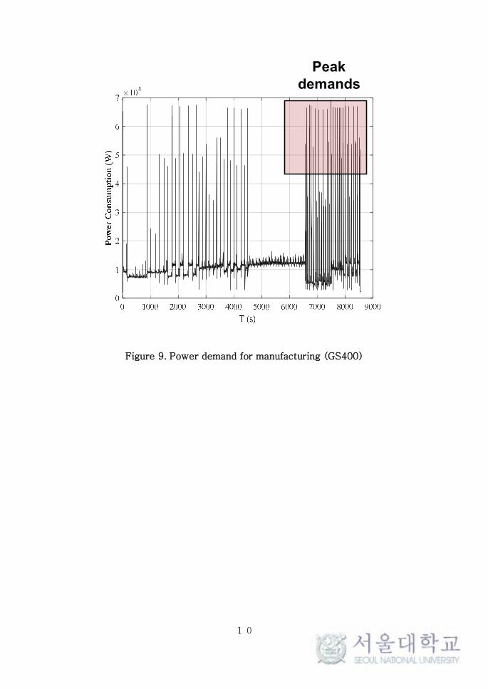
Figure 9. Power demand for manufacturing (GS400)

Peak demands

１１

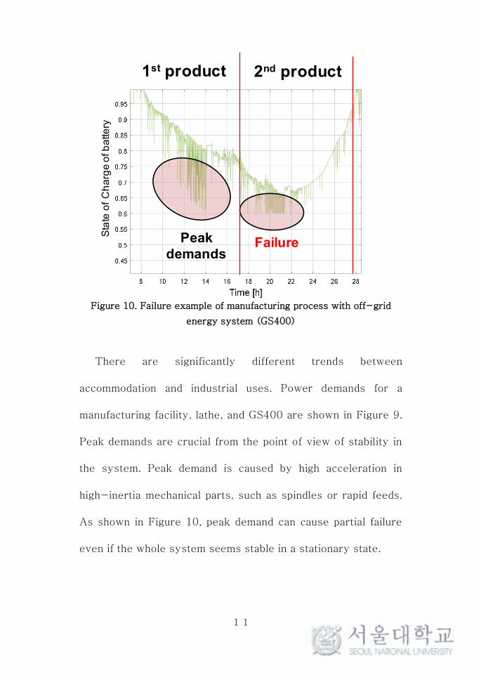
Figure 10. Failure example of manufacturing process with off-grid

energy system (GS400)

There are significantly different trends between

accommodation and industrial uses. Power demands for a

manufacturing facility, lathe, and GS400 are shown in Figure 9.

Peak demands are crucial from the point of view of stability in

the system. Peak demand is caused by high acceleration in

high-inertia mechanical parts, such as spindles or rapid feeds.

As shown in Figure 10, peak demand can cause partial failure

even if the whole system seems stable in a stationary state.

Peak demands

Failure

1st product 2nd product

Sta

te o

f C

ha

rge

of b

atte

ry

１２

2 Renewable energy production model

Several researchers have used the Hybrid Optimization of

Multiple Energy Resources (HOMER) to optimize the size of a

renewable energy plant [14]. Lal et al. optimized a hydro mini-

grid system with HOMER [15]. Chong et al. calculated the

appropriate scale of an autonomous hybrid wind/photovoltaic

(PV)/battery power system for a household [16]. There are

also 68 tools for analyzing renewable energy systems [17].

2.1 PV energy production

PV is the primary source of energy generation in off-grid

systems. A PV array can be used with a grid-tied inverter

(GTI) with a main grid [10]. However, most off-grid cases

require battery banks [13, 18-26].

2.1.1 Mathematical models and patterns of energy

production

There are three major types of PV model for estimating PV

potential [27-31]. An ideal single-diode PV cell model was

derived from the theory of semiconductors and this model has

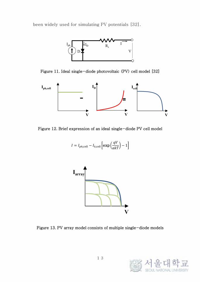
１３

been widely used for simulating PV potentials [32].

Figure 11. Ideal single-diode photovoltaic (PV) cell model [32]

Figure 12. Brief expression of an ideal single-diode PV cell model

Figure 13. PV array model consists of multiple single-diode models

V

Iph,cell

V

ID

V

Icell

- =

V

Iarray

= , − , exp

− 1

１４

Iph,cell and I0,cell are the PV and saturation current of cell and

Iph and I0 represent the array of PV. q is the electron charge

(1.60218 × 10-19 C), V is the potential of the PV, a is the

diode ideality constant, k is the Boltzmann constant (1.38065

× 10-23 J/K), and T is the temperature of the cell.

A PV array model is obtained with the ideal single-diode PV

cell model equation. In this research, the PV array model is an

implicit equation and the Newton– Raphson method was used to

obtain the I-V curve for the target system. Error tolerance was

defined as 0.001 and range of voltage is larger than 0 V, I = Isc

condition, to Voc, I = 0.

Simulation conditions were defined with specification of the

= −(, )

(, )

, 0 < < , Newton − RaphsonMethod

= −1 −

t

exp +

t −

s

= 0

(, ) = − + − exp +

t − 1 −

+ s

= 0

= − exp +

t − 1 −

+ s

１５

target PV panel, SSP-120D, and I-V curve. Figure 14 was

obtained from the proposed model and power performance and

maximum power were obtained as shown in Figure 15.

１６

Figure 14. Typical I-V curve for an array of PVs

Figure 15. Typical power curve for an array of PVs

(0,Isc)

(Vos,0)

(Vmp, Imp)

１７

To verify the modeling results, the maximum power of the

PV was measured with the conditions indicated in Table 1. The

measured solar irradiation value and current were 307.6 W/m2

and 6.51 A, respectively. The rated current was 6.89 A and the

three solar panels are in series, so that the rated current is

equal to 20.67 A. The PV current is proportional to solar

irradiation so that the estimated current is equal to 6.36 A.

１８

Figure 16. Experimental result of PV model verification

Table 1. Verification parameters of the PV array

Model SSP-120D

Ratedpower 120W

Shortcircuitcurrent 7.63A

Opencircuitvoltage 21.75V

Max power generation point

307.6 W/m2

6.51 A

１９

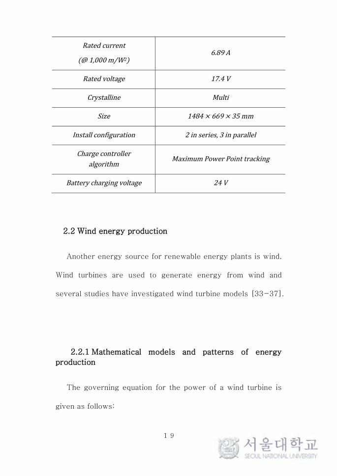
Ratedcurrent

(@1,000m/W2)6.89A

Ratedvoltage 17.4V

Crystalline Multi

Size 1484× 669× 35mm

Installconfiguration 2inseries,3inparallel

Chargecontroller

algorithmMaximumPowerPointtracking

Batterychargingvoltage 24V

2.2 Wind energy production

Another energy source for renewable energy plants is wind.

Wind turbines are used to generate energy from wind and

several studies have investigated wind turbine models [33-37].

2.2.1 Mathematical models and patterns of energy

production

The governing equation for the power of a wind turbine is

given as follows:

２０

Pw is the power generated from the wind turbine (W), CPU is

the power coefficient, A is the intercepting area of the rotor

blades (m2), V is the average wind speed (m/s), and λ is the

tip speed ratio. Coefficients of Cp were obtained from

experimental data [34, 38]. A typical power curve for a wind

turbine is shown in Figure 17.

=

1

=

1

+ 0.08−0.035

+ 1

(, ) = − −

+

=1

2(, )

２１

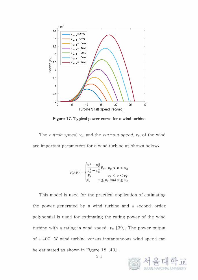
Figure 17. Typical power curve for a wind turbine

The cut-in speed, vC, and the cut-out speed, vF, of the wind

are important parameters for a wind turbine as shown below:

This model is used for the practical application of estimating

the power generated by a wind turbine and a second-order

polynomial is used for estimating the rating power of the wind

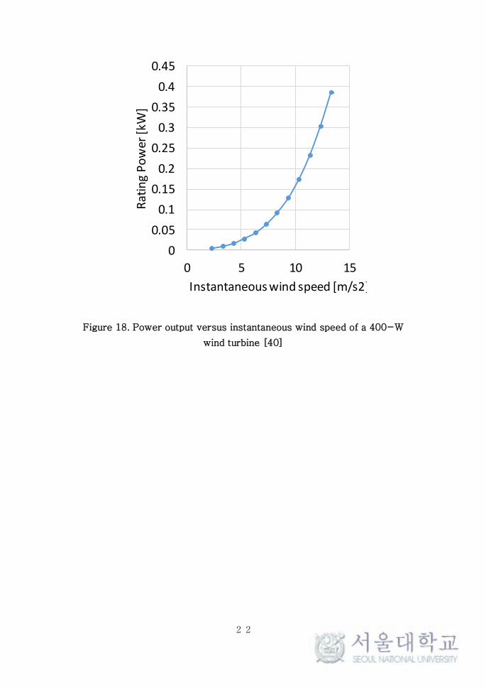
turbine with a rating in wind speed, vR [39]. The power output

of a 400-W wind turbine versus instantaneous wind speed can

be estimated as shown in Figure 18 [40].

() =

⎩⎪⎨

⎪⎧

−

−

, < <

, < < 0, ≤ ≥

２２

Figure 18. Power output versus instantaneous wind speed of a 400-W

wind turbine [40]

0

0.05

0.1

0.15

0.2

0.25

0.3

0.35

0.4

0.45

0 5 10 15

Rat

ing

Po

wer

[kW

]

Instantaneous wind speed [m/s2]

２３

2.3 Battery model

A battery is a major component of off-grid renewable

energy systems. Renewable energy sources are so random that

renewable power plants are eventually overdesigned. To

minimize the instability of renewable energy systems, a set of

batteries was installed with PV arrays and wind turbines.

In this research, a manufacturing-oriented off-grid

renewable energy system requires much higher stability so a

battery model is much more important than in ‘conventional’

research.

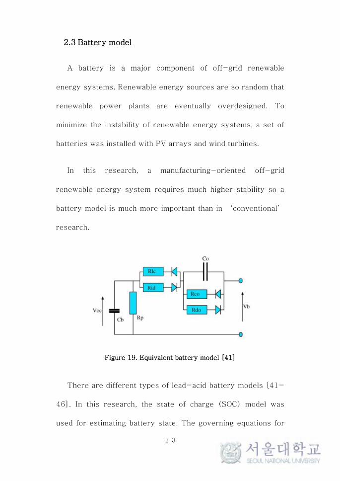
Figure 19. Equivalent battery model [41]

There are different types of lead-acid battery models [41-

46]. In this research, the state of charge (SOC) model was

used for estimating battery state. The governing equations for

２４

SOC involve integrating current flow through the battery and

integrating current to charge. The maximum SOC is limited by

the capabilities of the battery. Furthermore, there are internal

resistances calculated by the SOC so that when the SOC is low,

internal resistance is high, and the external voltage is low

spontaneously.

VOC is the open circuit voltage of the battery, S is the state

of charge factor (form 0, for fully discharged; up to 1 for fully

charged), k is the capacity coefficient, R0 is the resistance of

the fully charged battery (Ω), and C10 is the 10-h capacity (Ah)

at a reference temperature, commonly 25°C. For a dynamic

model, considering charging and discharging models, the

additional terms RLc, Rid, Rco, and Rdo are added in both

directions of current flow (Figure 19).

= =

, where = lowervoltageboundary

= () ≥ 0, − ()( + )

() < 0, −()( +)

= 1 −∫()

(, )

=

２５

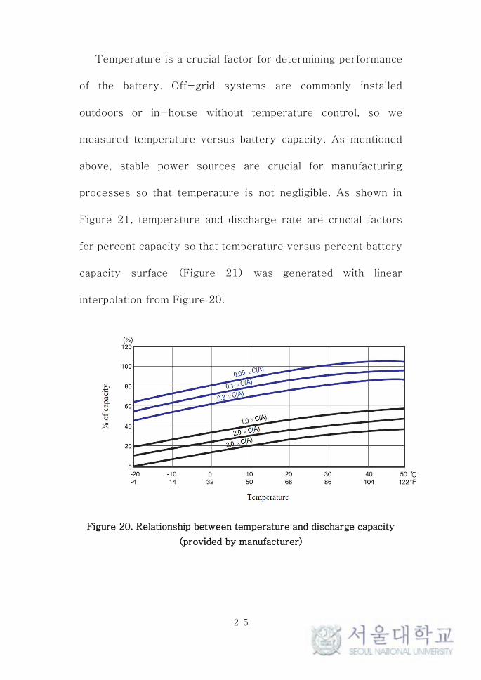
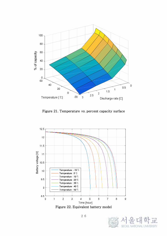
Temperature is a crucial factor for determining performance

of the battery. Off-grid systems are commonly installed

outdoors or in-house without temperature control, so we

measured temperature versus battery capacity. As mentioned

above, stable power sources are crucial for manufacturing

processes so that temperature is not negligible. As shown in

Figure 21, temperature and discharge rate are crucial factors

for percent capacity so that temperature versus percent battery

capacity surface (Figure 21) was generated with linear

interpolation from Figure 20.

Figure 20. Relationship between temperature and discharge capacity

(provided by manufacturer)

２６

Figure 21. Temperature vs. percent capacity surface

Figure 22. Equivalent battery model

% o

f capacity

Ba

tte

ry v

olta

ge

[V

]

２７

Combining the SOC model and temperature versus percent

capacity model, an equivalent battery model with temperature

was developed. As shown in Figure 22, the lower the

temperature, the faster the drop in external voltage. A

monitoring platform measured the current flow of the battery

and the SOC could be obtained by integrating current flow to

the battery.

２８

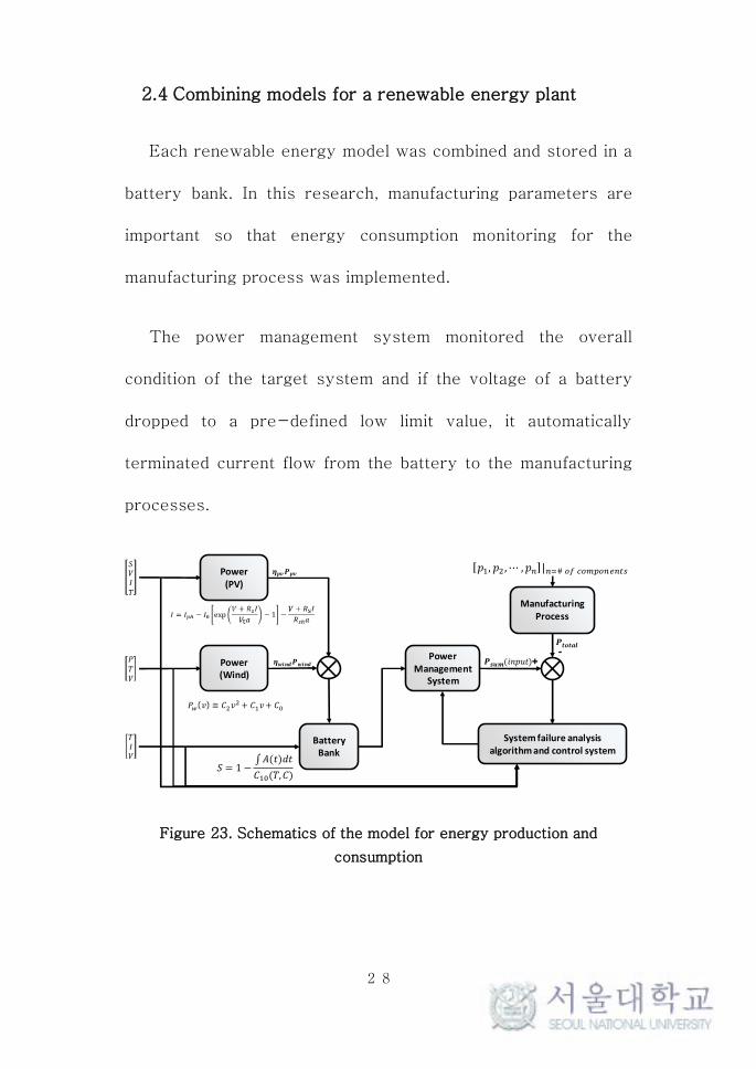
2.4 Combining models for a renewable energy plant

Each renewable energy model was combined and stored in a

battery bank. In this research, manufacturing parameters are

important so that energy consumption monitoring for the

manufacturing process was implemented.

The power management system monitored the overall

condition of the target system and if the voltage of a battery

dropped to a pre-defined low limit value, it automatically

terminated current flow from the battery to the manufacturing

processes.

Figure 23. Schematics of the model for energy production and

consumption

Power(PV)

Power(Wind)

ManufacturingProcess

-+

, , ⋯ , |#

PowerManagement

System

()

System failure analysisalgorithm and control system

BatteryBank

= 1 −∫()

(,)

≅ + +

２９

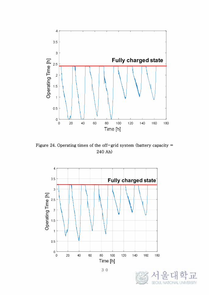
2.5 Operation time calculations

Operating time calculations were studied with energy

production and a consumption model according to the following

equation:

=(, ) − () − ()

()

∙ =(, ) − () − ()

∙

ℎ, () − () ≠ 0

test is the estimated operation time of the off-grid renewable

energy system and SOCfail is a failure condition of the battery

bank. Igen and Iman denote the current flow of power generation

and manufacturing. If Igen is larger than Iman, energy is stored in

the battery bank so that operating time increases until the

battery bank is fully charged. Furthermore, current flow also

affects the operating time. Operating time and instantaneous

operating time can be calculated as shown in Figure 24 and

Figure 25, respectively.

３０

Figure 24. Operating times of the off-grid system (battery capacity =

240 Ah)

Fully charged state

Op

era

tin

g T

ime [

h]

Fully charged state

Op

era

tin

g T

ime [

h]

３１

Figure 25. Operating times of the off-grid system (battery capacity =

320 Ah)

2.6 Conclusions

A renewable power model was reviewed and implemented to

a renewable energy system simulator. Manufacturing power

consumption was also considered to determine the stability of a

manufacturing-oriented simulation. Furthermore, an operation

time calculation algorithm was implemented.

３２

3 Manufacturing energy consumption model

Conventional manufacturing processes require stable power

sources. However, if a power source is not stable, such as an

off-grid renewable energy system, estimating the power

demand of the manufacturing process is crucial. Worldwide, the

ratio of renewable energy sources is increasing so that it will

be necessary to predict energy consumption in manufacturing

processes. In this section, power demands for a manufacturing

process were determined and modeled with process and

empirical parameters of each manufacturing process: in this

case, the lathe.

3.1 Overview

Energy efficiency has become an increasingly important

issue in industry due to growing energy costs and

environmental concerns [47]. Much research has been carried

out with the aim of reducing the energy consumption of machine

tools, using both experimental and theoretical methods. From

the viewpoint of productivity, Dornfeld [48] developed an

“eco-route map” that described the concept of improved

３３

manufacturing processes and systems. Kara et al. [49] used the

specific energy consumption (SEC) model for various work

piece materials and machine tools. Yoon et al. [50] measured

the power required for cutting, including tool wear, using the

response-surface method (RSM). Gutowski et al. [51]

proposed an energy framework to describe manufacturing

processes, and the EnergyBlock planning method was proposed

by Weinert et al. [52] to reduce the total energy consumption

of manufacturing processes. Dietmair [53] studied the

efficiency of machining processes using an energy consumption

model. Xu et al. [54] developed a theoretical model to describe

the required cutting power of machine tools, considering

empirical coefficients as well as the geometric variables of the

tool. Lee et al. [55] developed a detailed model describing the

mechanical and electronic coefficients of a feed-drive system.

Yoon et al. [56] compared the energy consumption of

manufacturing processes, including bulk forming, cutting, and

rapid prototyping.

As part of recent efforts to standardize the energy

consumed by machine tools, the International Organization for

Standardization (ISO) developed the ISO 14995 series of

３４

standards [4]. The first part of these standards defines the

design parameters of machine tools that affect energy

consumption. The second part, which is still under development,

describes energy consumption measurement procedures. The

Japanese Standard Association (JSA) also developed standard

power measurement procedures and specimens for cutting

processes [57]. The JSA standard specimen for a three-axis

milling machine was used by Min et al. [58] to calculate the

energy consumption of machine tools of various sizes.

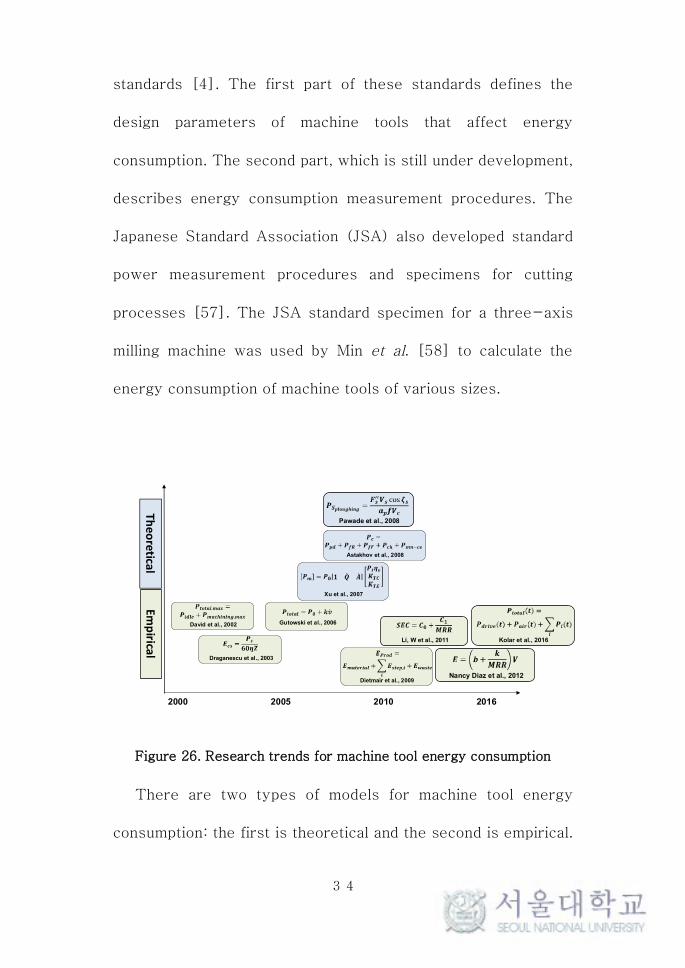
Figure 26. Research trends for machine tool energy consumption

There are two types of models for machine tool energy

consumption: the first is theoretical and the second is empirical.

Theo

reticalEm

pirical

2000 2005 2010 2016

David et al., 2002

Draganescu et al., 2003

Gutowski et al., 2006

Xu et al., 2007

Astakhov et al., 2008

Dietmair et al., 2009

Pawade et al., 2008

Li, W et al., 2011

Nancy Diaz et al., 2012

Kolar et al., 2016

３５

There are few theoretical models for machine tools and cutting

power [54, 59, 60], and there are several empirical models.

Because of the complexity of machine tool configurations and

mechanical properties, an empirical model is commonly used to

estimate energy consumption of machine tools.

The literature reviewed above describes various empirical

approaches and measurement procedures. However, the

development of standardized processes has been hindered by

the number of parameters and the complexity of the procedures.

For these reasons, we describe a simplified measurement

method that integrates the feed drive, the spindle, and cutting.

Six different machine tools were examined to verify the

accuracy of the model.

3.2 Theoretical backgrounds on manufacturing energy

consumption

The EnergyBlock method of Weinert et al. [52] was used to

measure the energy consumption of the machine tool itself

using the following two expressions:

３６

() =

()∀ ∈ [ , ]

()∀ ∈ [, ]…

()∀ ∈ [, ]

and

= ()

where fn is the power profile within the time interval Tn-1 to

Tn, Pp(t) is the power profile function, and Ep is the energy,

which can be calculated by integrating Pp(t) from T0 to T1.

A first-order polynomial energy model for the spindle and

feed drive was assumed for simplicity [55, 61]. The SEC is

widely used to describe the cutting energy. If the work piece

material is known, then the SEC is a powerful tool to calculate

the cutting energy, even though this varies with the cutting

force, which is related to the cutting speed, the coolant, and the

tool geometry. In this study, the cutting energy consumption

was estimated using the material removal rate (MRR) model,

inspired by the models of Kara et al. and Dornfeld et al. [49,

62], and the cutting energy consumption was decomposed using

model equation 3, as suggested by Gutowski et al. [51].

３７

= +

where

⎩⎨

⎧ = =

= ℎ/

= , ℎ/

Here, we use the following basic form of the power model:

() = ∙ +

where Pp(α) is the power consumption of peripherals, such

as idle, coolant, machining, spindle, and feed drive.

= + + + +

, ℎ

⎩⎪⎨

⎪⎧

= =

= ∙ + = ∙ + = ∙ +

In this manner, the power consumption of the machine tool is

modeled as the sum of five terms: the power consumption for

idle PIdle, the power consumption of the coolant system PCoolant,

the spindle power consumption PSpindle, the feed drive power

consumption Pied, and the cutting power consumption PMachining.

C0s, C1f, and C0m are the gradients of the power model of the

cutting, spindle, and feed drive, respectively, and C1i and C1c are

３８

the power offset coefficients for idling and/or the coolant pump.

3.2.1 Cutting process energy consumption model

Before obtaining cutting energy consumption, cutting force

should be determined. Cutting force Fc can be calculated by

Merchant’s circle, where Fc is the vector summation of Fs,

resistance to shear of the metal in forming the chip, and F is the

frictional resistance of the tool acting on the chip (Figure 27).

In total, this is 70– 80% of the total force and it is parallel to

the velocity of the tool relative to the work piece so that the

cutting force Fc is a major factor in the energy consumption of

the cutting process. Thus, cutting power, P, can be calculated

with cutting force, Fc, and cutting speed, V.

Figure 27. Cutting force diagram

FC : Tangential ‘Cutting’ Force

FT : Longitudinal

‘Thrust’ Force Fr : Radial

Force

Cutting Tool

Direction of Feed

Workpiece

V :Velocity of tool relative to workpiece

=

３９

Figure 28. Merchant’s circle

Because of the complexity of the Fc calculation, the SEC

model is commonly used for estimating the required energy for

the cutting process. The SEC model is a simpler form of the

cutting power model, rather than power calculated by cutting

force if the cutting force is constant.

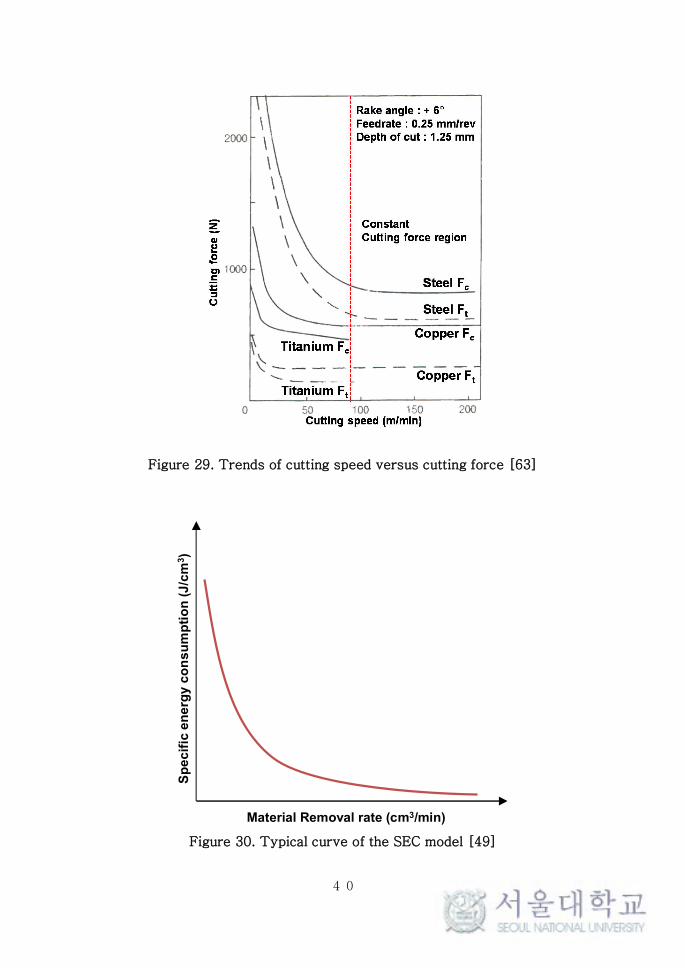
As shown in Figure 29, cutting force is constant with over

90 m/min of cutting speed [63]. Thus, if the cutting speed is

high enough, the SEC model can be applied to estimate the

cutting energy consumption.

R

N

F

Fc

Fs

Fn

Ft

α

α

Ф

Ф

λ

λ-α

Tool

V

４０

Figure 29. Trends of cutting speed versus cutting force [63]

Figure 30. Typical curve of the SEC model [49]

Material Removal rate (cm3/min)

Sp

ec

ific

en

erg

y c

on

su

mp

tio

n (

J/c

m3)

４１

The SEC model has two empirical variables, C0 and C1. A

typical curve of the SEC model is shown in Figure 30 and the

SEC model has been implemented by previous researchers [49,

50, 62, 64-66]. Two empirical variables should be obtained by

experimental results within the constant cutting force region.

Tool wear is directly related to cutting force [50], so tool

manufacturers provide high-cutting-speed conditions.

∙ = ∙ + =

= +

４２

3.2.2 Feed drive friction-based energy consumption

model

For feed drive units, Lee et al. proposed a component-based

friction model for estimating the energy demands of a machine

tool [55]. Based on the friction model, power loss of the feed

drive unit can be summarized as shown in Table 2.

Table 2. Composition and power losses of the feed drive system [55]

As Lee et al. mentioned power loss of each component, a

common term for power loss at each component is feed rate.

The following equations are described in [55]:

Component Losses Factors Output

Motor drive - - Driving power

Motor

ElectricalLoss (PM1)

Idling lossCopper loss

Iron loss

Driving torque of the motor

Mechanical loss (PM2)

Inertial forceDamping forceFriction force

Torque used to drive the ball

screw

Ball screwMechanical

loss (PB)Inertial forceFriction force

Force used to drive the table

Table with LM guide

Mechanical loss (PL)

Inertial forceFriction force

Table position

= 2( − )/

= − 2/

４３

3.3 Standardized energy consumption measurement

procedure

3.3.1 Assumptions and experimental design

Most existing methods that describe the energy consumption

of machine tools are based on the concept of a standardized

work piece; however, it is not always straightforward to use

such a standardized work piece for an arbitrary machine tool

because of the wide variety of types and configurations of

machine tools. The energy consumed during cutting depends on

several factors, including the work piece material, the cutting

features, the tool material, the geometry, and the type of

machine tool. This large number of factors complicates the

development of a unified model. There has been substantial

research into models of the cutting process and energy

consumption during the cutting process using existing cutting

, ℎ

⎩⎪⎨

⎪⎧

: :

: ℎ : ℎ

:

=

= (2/ − )

４４

models.

An objective of this work was to separate the cutting energy

from the energy consumption of machine tools, because the

contribution of the machine tool to the cutting energy appears

to be determined by the characteristics of the machine tool

rather than the process. The cutting power consumption has

been estimated using the cutting force and cutting speed [67],

and the cutting force is proportional to the instantaneous feed

rate and depth of cut if a machine tool cuts the same material

with the same tool at a nominal cutting speed [68]; i.e., the

process condition is the dominant variable used to estimate

cutting power. If the energy consumption behavior of the

machine tool itself can be described separately, it can be used

to estimate the cutting energy. This method significantly

reduces the time and effort required for measurements and

modeling of the energy consumption of a machine tool, while

providing an accurate estimate of the energy used by the

machine tool, and the cutting energy.

The procedure consists of two steps. The first is to measure

the energy consumption without cutting (i.e., the energy of an

４５

air-cut), as well as the power consumption of the individual

components. The second is to measure the cutting energy using

the same sequence as in the first step to determine whether the

cutting energy can be decoupled from the energy used by the

machine tool without cutting.

４６

3.3.2 Data measurement and analysis procedure

The energy measurement procedure is as follows:

Step1. Initiateenergymeasurement

Step2. Idlestate:30s

Step3. Coolantpump:30s

Step4. Cutting,spindle, andfeeddrive

A. Spindleon

B. Cutting

C. Travel+x-axis

D. Travel – z-axis

E. Travel – x-axis

F. Changespindlespeed(withaconstantcuttingspeed)

G. Cutting

H. RepeatfromA

Step5. Spindleandcoolantoff

Step6. Endofenergymeasurement

A dwell time of 5 s is included between each step to identify

the times when the power profile changes. After defining the

start and end points of the profile, the power consumption was

calculated from the average of the profile, subtracted from the

average of the dwelling profile (i.e., the tare energy), which is a

widely used decomposition process [50, 66]. The power

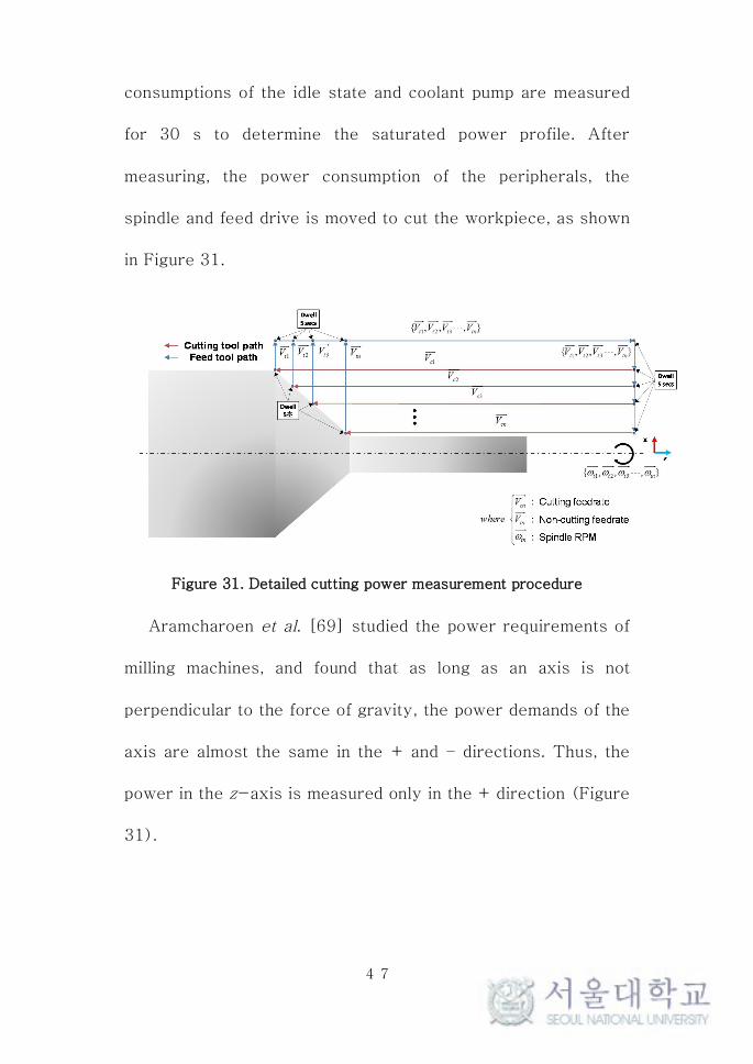
４７

consumptions of the idle state and coolant pump are measured

for 30 s to determine the saturated power profile. After

measuring, the power consumption of the peripherals, the

spindle and feed drive is moved to cut the workpiece, as shown

in Figure 31.

Figure 31. Detailed cutting power measurement procedure

Aramcharoen et al. [69] studied the power requirements of

milling machines, and found that as long as an axis is not

perpendicular to the force of gravity, the power demands of the

axis are almost the same in the + and – directions. Thus, the

power in the z-axis is measured only in the + direction (Figure

31).

４８

Figure 32. Example of a power profile and power measurement

procedure

Figure 33. Decomposition of additional electrical power requirement

In this study, the measurements of energy consumption

during the cutting, the spindle, and the feed-drive steps were

repeated 45 times to complete three sets of the Box– Behnken

1800 1802 1804 1806 1808

2000

3000

4000

5000

X: 1802

Y: 2774

T (s)

Po

wer

Con

sum

ptio

n (W

)

X: 1802

Y: 2774

X: 1807

Y: 2615

Additional electrical power

requirement

Measurement period

Reference electrical power

requirement

Transientstate

Transientstate

４９

experimental design. The speeds of the spindle and the +x, – x,

and – z feed drives were increased gradually to control the

cutting speed. The spindle speed was controlled to provide a

constant cutting speed, and the feed rate was increased from

3,250 to 5,000 mm/min at intervals of 250 mm/min. Table 1

lists the cutting conditions. Horizontal cutting was carried out

using 60-mm diameter AISI1045 mild steel rods, and a carbide

CNMG type insert tool, with a positive rake angle of 15°.

A Yokogawa WT330 digital power meter was used to

measure the energy consumption of the machine tool (Figure

34). The sampling rate was 10 Hz, and no low-pass filter was

used. Six different machine tools were investigated. Table 2

lists the specifications of these machines. Only the saturated

profiles were analyzed, to investigate the effects of over-

shooting the power profile for each component. Acceleration

and deceleration were neglected due to the low sampling rate.

The total power demand of the machine tool includes the

combined demands of the idle, coolant, spindle, feed drives, and

cutting power, which were determined individually. Thus, the

additional electrical energy required was calculated by

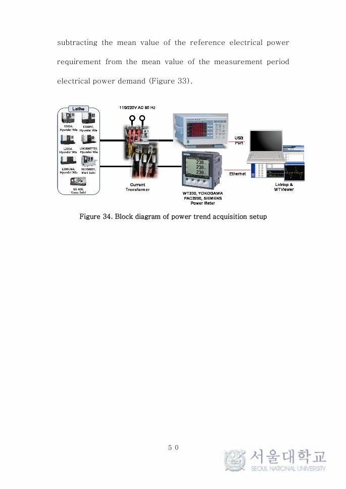
５０

subtracting the mean value of the reference electrical power

requirement from the mean value of the measurement period

electrical power demand (Figure 33).

Figure 34. Block diagram of power trend acquisition setup

５１

3.4 Results

The idle power consumption and the power consumption of a

coolant pump are related to the numerical controller and the

coolant pump itself. The idle power consumption and the power

consumption of a coolant pump are constants [52, 53, 58, 69].

Model coefficients were calculated from the experimental

results. The model results were fitted using linear regression,

as shown in Figure 36– Figure 37. The spindle power

consumption was fitted with a coefficient of determination of R2

> 0.9, and the cutting power consumption was fitted with a

coefficient of determination of R2 > 0.99. A value of R2 > 0.9

shows that the regression fit the data well.

Figure 35. Axis orientation of CNC lathe

The energy consumption of the spindle and the feed drive

Chuck

Spindle axis

Tool

Gravitational force direction

xz

Tool movement direction

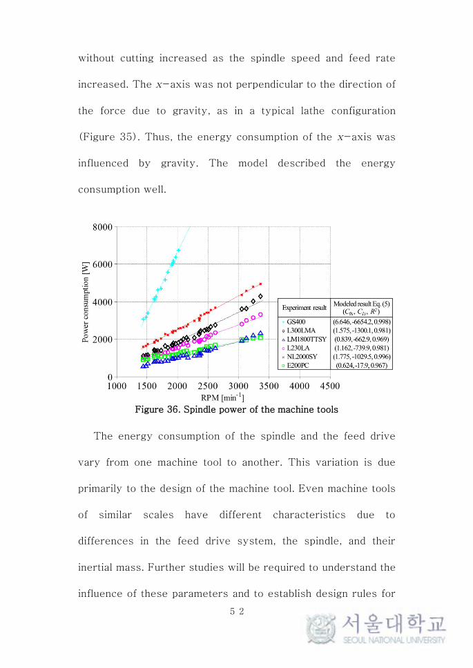
５２

without cutting increased as the spindle speed and feed rate

increased. The x-axis was not perpendicular to the direction of

the force due to gravity, as in a typical lathe configuration

(Figure 35). Thus, the energy consumption of the x-axis was

influenced by gravity. The model described the energy

consumption well.

Figure 36. Spindle power of the machine tools

The energy consumption of the spindle and the feed drive

vary from one machine tool to another. This variation is due

primarily to the design of the machine tool. Even machine tools

of similar scales have different characteristics due to

differences in the feed drive system, the spindle, and their

inertial mass. Further studies will be required to understand the

influence of these parameters and to establish design rules for

５３

‘green’ machines.

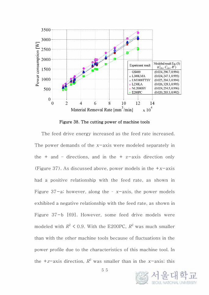
The cutting energy increased as the MRR increased and

varied linearly with the MRR (Figure 38). The cutting energy

varied little between the six machines, although these machine

tools had different specifications. This suggests that the cutting

energy is not strongly dependent on the design or components

of the machine tool. Thus, the cutting energy can be decoupled

from the characteristics of the machine tool, and the models for

the spindle and the feed drive can be used as inputs to the

cutting-energy model. The most interesting trend in the cutting

power consumption occurred when the machine tool was

equipped with a controller from Fanuc Corporation. In particular,

the five machine tools (i.e., GS400, L230LA, L300LMA,

NL2000SY, and LM1800TTSY) exhibited very similar cutting

power consumption models because the gradients of the cutting

power consumption model, C0m, were nearly the same.

５４

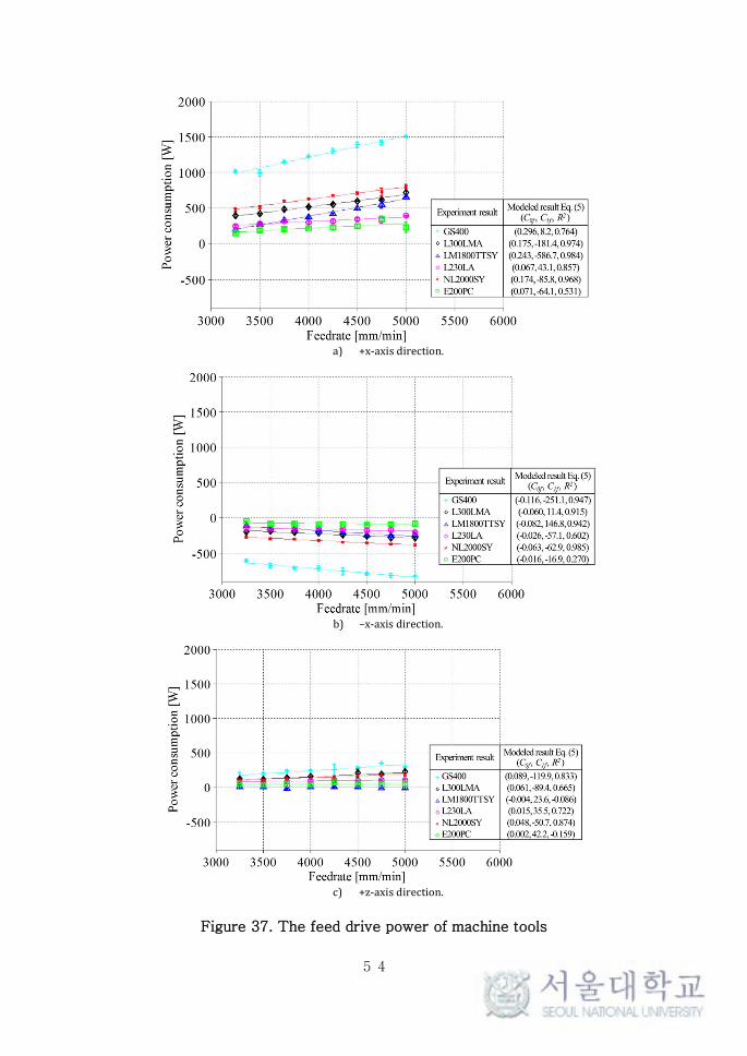
a) +x-axis direction.

b) –x-axis direction.

c) +z-axis direction.

Figure 37. The feed drive power of machine tools

５５

Figure 38. The cutting power of machine tools

The feed drive energy increased as the feed rate increased.

The power demands of the x-axis were modeled separately in

the + and – directions, and in the + z-axis direction only

(Figure 37). As discussed above, power models in the +x-axis

had a positive relationship with the feed rate, as shown in

Figure 37-a; however, along the – x-axis, the power models

exhibited a negative relationship with the feed rate, as shown in

Figure 37-b [69]. However, some feed drive models were

modeled with R2 < 0.9. With the E200PC, R2 was much smaller

than with the other machine tools because of fluctuations in the

power profile due to the characteristics of this machine tool. In

the +z-axis direction, R2 was smaller than in the x-axis; this

５６

was because the signal-to-noise ratio in the z-axis was larger

than that in the x-axis due to the larger power consumption in

the x-axis.

５７

3.5 Energy consumption simulator

3.5.1 Overview

The power consumption of a machine tool depends on the

control parameters, including the NC code. The power

consumption of each component is separated in the model;

however, the power consumption of machine tools is the sum of

each of the peripherals. Thus, we should sum the contributions

from the different components of the model to describe overall

power consumption of the machine tool. In this section, we

describe the power profile simulation method.

The first step of this model is to export the operating

conditions for the machine tool. The machine tool operating

information is analyzed as a time-based array. The time

information is calculated from the position and feed rate data. In

the model, we require only the times when the peripherals’

conditions change.

The second step is to include the machine tool operating

conditions matrix in the time information array. We use the

models in Equation 5, which require operating parameters with

５８

a time array. The feed rates for each axis are linearly

interpolated. The feed rates for each axis are calculated as a

function of the position.

５９

3.5.2 Simulation procedure and results

The model was confirmed using a simulation tool. The power

profile simulation was composed of an NC code analyzer and a

time-wise power profile solver. The total power consumption

of the machine tool can be calculated as the sum of each of the

components of the power consumption model; i.e.,

(, , , ) = , + ,

+ , ,

, + , , ,

ℎ =

⋯

=

⎣⎢⎢⎢⎢⎢⎢⎡ ∙

1

||

∙1

||⋯

∙1

|| ⎦⎥⎥⎥⎥⎥⎥⎤

, =

⎣⎢⎢⎢⎡//

⎦

⎥⎥⎥⎤

, =

, =

⎣⎢⎢⎢⎢⎡

⎦

⎥⎥⎥⎥⎤

#

/ = 1, ≥ 0, <

Information on the operation of the machine tool was

imported from the NC code. The power consumption model was

developed using the operating conditions included in the NC

code. Thus, the power profile simulator required only the NC

code, the cutting variables, and the MRR. The NC code contains

６０

only point-to-point position and feed rate data, and the NC

controller interpolates velocities to drive the stage to the

desired positions. The power consumption model contains the

power consumption for each axis and at each feed rate

independently, and interpolated velocities were calculated using

the following expression:

⎣⎢⎢⎢⎡

⎦

⎥⎥⎥⎤

=

⎣⎢⎢⎡ ( ∙ )

( ∙ )

( ∙ ) ⎦

⎥⎥⎤

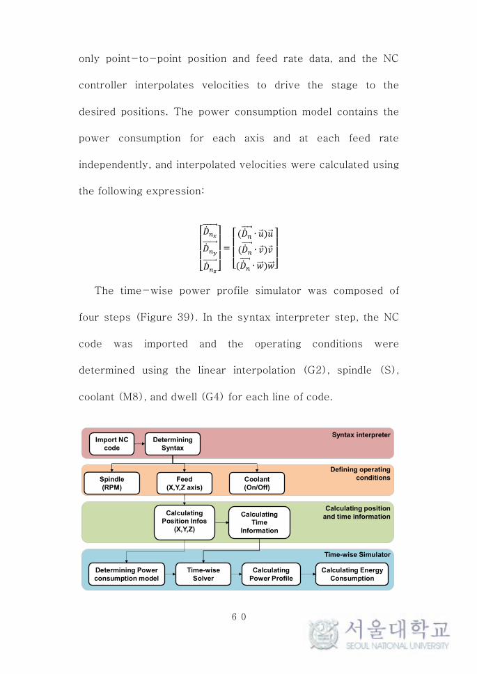
The time-wise power profile simulator was composed of

four steps (Figure 39). In the syntax interpreter step, the NC

code was imported and the operating conditions were

determined using the linear interpolation (G2), spindle (S),

coolant (M8), and dwell (G4) for each line of code.

Import NC code

DeterminingSyntax

Spindle(RPM)

Feed(X,Y,Z axis)

Coolant(On/Off)

Calculating Position Infos

(X,Y,Z)

Calculating Time

Information

Time-wiseSolver

Calculating Power Profile

Determining Power consumption model

Calculating Energy Consumption

Syntax interpreter

Defining operating conditions

Calculating position and time information

Time-wise Simulator

６１

Figure 39. Flow chart describing the power profile simulation

After defining the syntax, the conditions of each of the

components were defined using the condition array,. Positions

and time data were then calculated using the feed information

as follows and shown in Figure 40:

Figure 40. Definition of the feed drive position vector

= ( − ) + ( − )

+ ( − )

=

=

∙ =

∙ (( − )

) + (( − ))

∙ =

∙ (( − )

) + (( − ))

( , , )n n n nP x y zuur

1 1 1 1( , , )n n n nP x y z+ + + +

uuur

1( , , )n n n n n nD X Y Z P P+= -uur uuur uur

xy

z

６２

∙ =

∙ (( − )

) + (( − ))

The power profile simulator was used to calculate the power

consumption of each component from the beginning to the end

of each time step. We used a time step of 0.1 s.

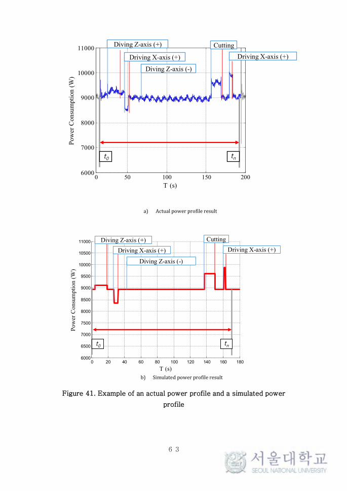
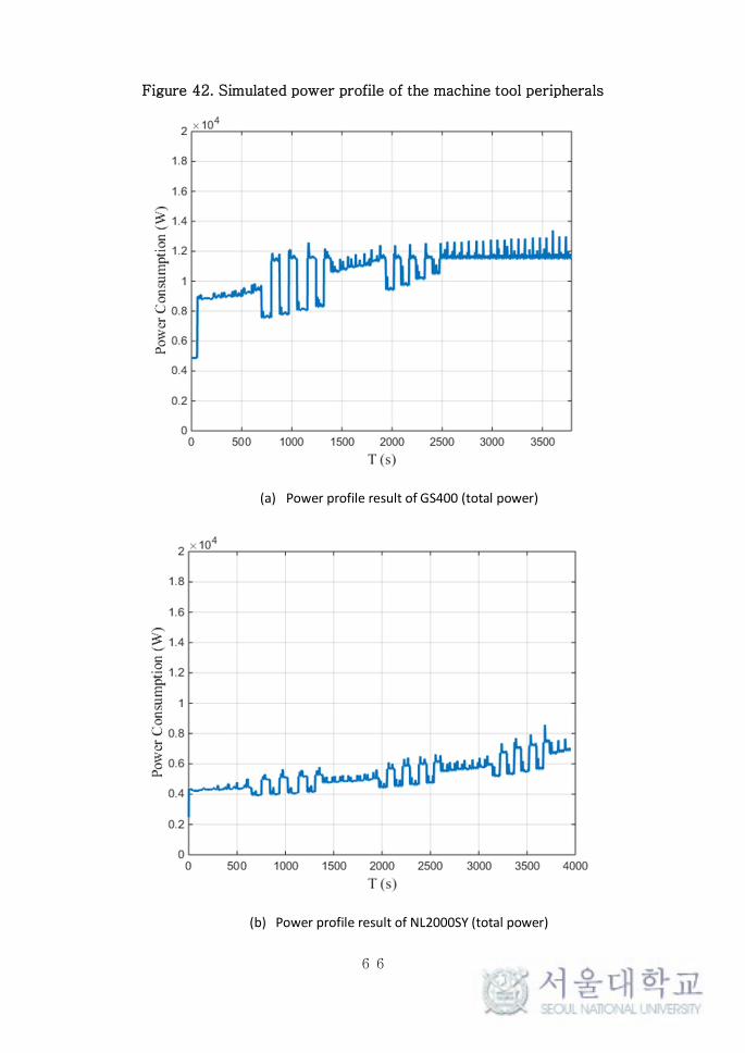
The power profile simulator was used to calculate the power

consumption of each of the peripherals at each time step.

Figure 41 shows that the actual power profile and simulated

power profile fit well. Figure 42 shows the power profile of the

machine tool peripherals. The idle power consumption was

constant at the beginning of the simulation. As the spindle

speed changed, the power consumption of the feed drive

changed depending on the feed rate. The sum of the peripherals

was equal to the total power consumption (Figure 41).

６３

a) Actual power profile result

b) Simulated power profile result

Figure 41. Example of an actual power profile and a simulated power

profile

1050 1100 1150 12006000

7000

8000

9000

10000

11000Experiment #analized62173

T (s)

Po

wer

Co

nsu

mp

tio

n (

W)

t0 tn

Diving Z-axis (+)

Driving X-axis (+)

Cutting

Driving X-axis (+)

Diving Z-axis (-)

0 50 100 150 200

0 20 40 60 80 100 120 140 160 1806000

6500

7000

7500

8000

8500

9000

9500

10000

10500

11000

T (s)

Po

wer

Co

nsu

mp

tio

n (

W)

t0 tn

Diving Z-axis (+)

Driving X-axis (+)

Cutting

Driving X-axis (+)

Diving Z-axis (-)

６４

To confirm the power model and the simulation method, we

simulated the total energy consumption of the GS400 and

NL2000SY machine tools, and compared values with the

measured energy consumption. The measured energy

consumption of the GS400 was 42.14 MJ, and that of the

NL2000SY was 20.54 MJ; the respective simulated energy

consumption values were 41.99 and 20.65 MJ. The power

consumption of the GS400 spindle did not exceed 6637.8 W,

due to the maximum spindle speed of 2,000 RPM. The

simulated total energy consumption of the GS400 was in

agreement with the measured result to within 0.36%, and the

simulated total energy consumption of the NL2000SY was in

agreement with the measured data to within 0.55%. Although

the total energy consumption of the NL2000SY was much less

than that of the GS400, the process times of the two machines

were similar, and the machining power consumption did not

differ significantly between the two machines.

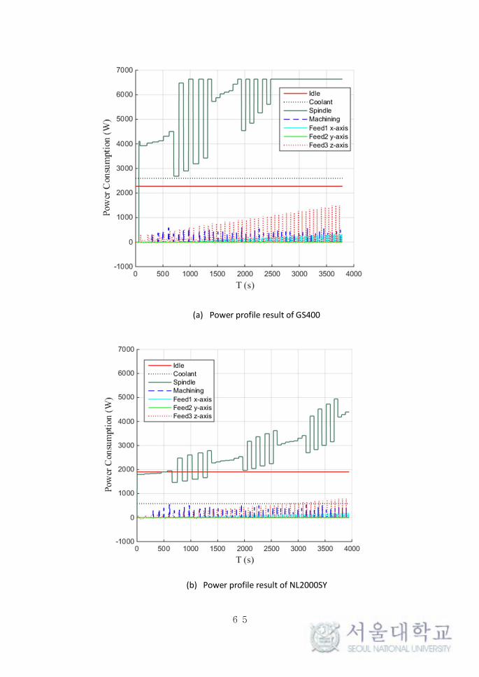
６５

(a) Power profile result of GS400

(b) Power profile result of NL2000SY

６６

Figure 42. Simulated power profile of the machine tool peripherals

(a) Power profile result of GS400 (total power)

(b) Power profile result of NL2000SY (total power)

６７

Figure 43. Simulated power profile of the machine tools

From the simulated data, the spindle power coefficient,,

was much larger for the GS400 than the NL2000SY; however,

the difference in the power trend coefficient is not necessarily

an indicator of a greener machine tool, and criteria describing

how green a given machine tool is should consider the scale and

use of the machine.

６８

3.6 Machine learning-based energy consumption

modeling

3.6.1 Overview

A time-wise simulator could obtain the power consumption

of a machine tool. However, the overall procedure of modeling

requires aborting an ongoing process and attempting the

proposed measurement procedure. Thus, a machine learning-

based modeling methodology is one solution for obtaining a

power model of the manufacturing process.

3.6.2 Physical model-based neural network design

In section 0, power trends of manufacturing processes could

be obtained by a summation of first-order polynomial functions

with process parameters, which is described in the NC code.

Thus, the power can be simplified with the following equation:

, , … , = + + +⋯+

６９

Based on the form of the equation above, an artificial neural

network (ANN) with a pure line function was used as a transfer

function of the network and the output form of the network is

equal to the power model. Labeled data sets were generated

with the simulator and training.

Figure 44. Block diagram of a two-layer artificial neural network (ANN)

[70]

= (( + ) + )

, =

, , , = ∙ +

, ,

, =

∙ +

,,

, = ∙ +

, =

７０

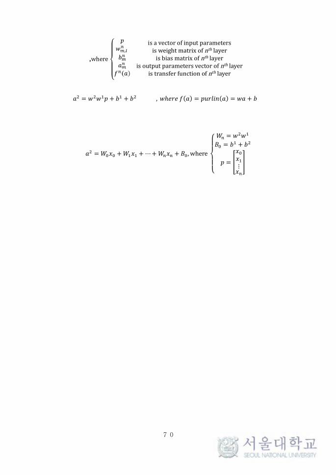
,where

isavectorofinputparametersisweightmatrixofnth layerisbiasmatrixofnth layer

isoutputparametersvectorofnth layeristransferfunctionofnth layer

= + +⋯+ +, where

⎩⎪⎨

⎪⎧ =

= +

=

⋮

, ℎ() = () = + = + +

７１

3.6.3 Backpropagation algorithm

To train the hidden layer of the ANN, a backpropagation

algorithm was implemented.

3.6.4 Results

ANN training parameters are described in Table 3. Six input

neurons are for manufacturing operation conditions and only

one output neuron is for the power demand for manufacturing at

the last layer of the ANN. The number of hidden layers is 100,

which is considered a high level. The initial learning rate is low

F(n) =

()0

0(

)

……

00

⋮ ⋮ ⋮0 0 … (

)

s = F(n)W

s, = − 1,… ,2,1

s = −2F(n)(t− a)

b( + 1) = b() −

s

W( + 1) = W() −

s

a

７２

because of the highly sensitive variables due to the Purelin

function. At first, the state of training, all weights, and biases

are initiated with random variables so that the error in the first

state is high and the backpropagation algorithm is easily

unstable. Thus, the learning rate of the designed ANN would be

low.

Table 3. ANN design and training parameters

Nameofvariable Value Note

Numberoflayer 3 -

Numberofinput

neurons6

6 operating

parameters

Numberofoutput

neurons1

Onlypower

obtained

Numberofhidden

neurons100

Highlevelof

degree

Transfer function Purelin()Duetophysical

model

Trainingdataset 2,000 Randomsamples

Verificationdataset 37,907Generatedby

simulator

Initiallearningrate 1.0 × 10-4 -

Learningrate 5.0 × 10-5Automatically

adjusted

７３

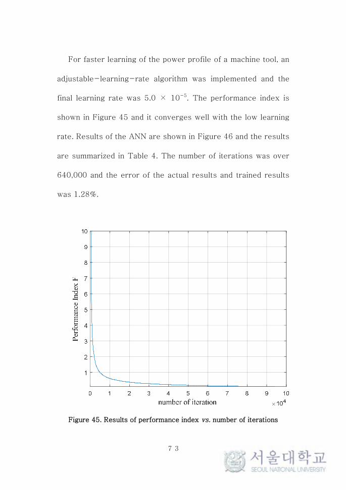
For faster learning of the power profile of a machine tool, an

adjustable-learning-rate algorithm was implemented and the

final learning rate was 5.0 × 10-5. The performance index is

shown in Figure 45 and it converges well with the low learning

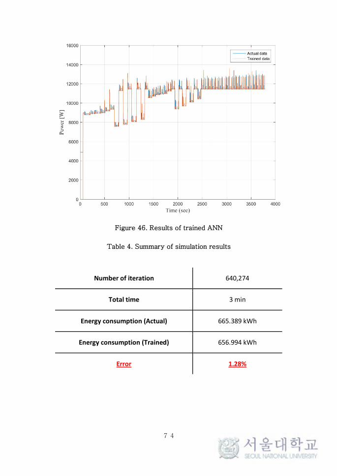
rate. Results of the ANN are shown in Figure 46 and the results

are summarized in Table 4. The number of iterations was over

640,000 and the error of the actual results and trained results

was 1.28%.

Figure 45. Results of performance index vs. number of iterations

７４

Figure 46. Results of trained ANN

Table 4. Summary of simulation results

Number of iteration 640,274

Total time 3 min

Energy consumption (Actual) 665.389 kWh

Energy consumption (Trained) 656.994 kWh

Error 1.28%

７５

3.7 Summary

An energy consumption model was investigated and modeled

with process parameters. The proposed model showed high

accuracy and a simulator was implemented. Moreover, a

physical model-based ANN was proposed and training results

fit the actual results well.

７６

4 Energy model for renewable energy and

manufacturing processes

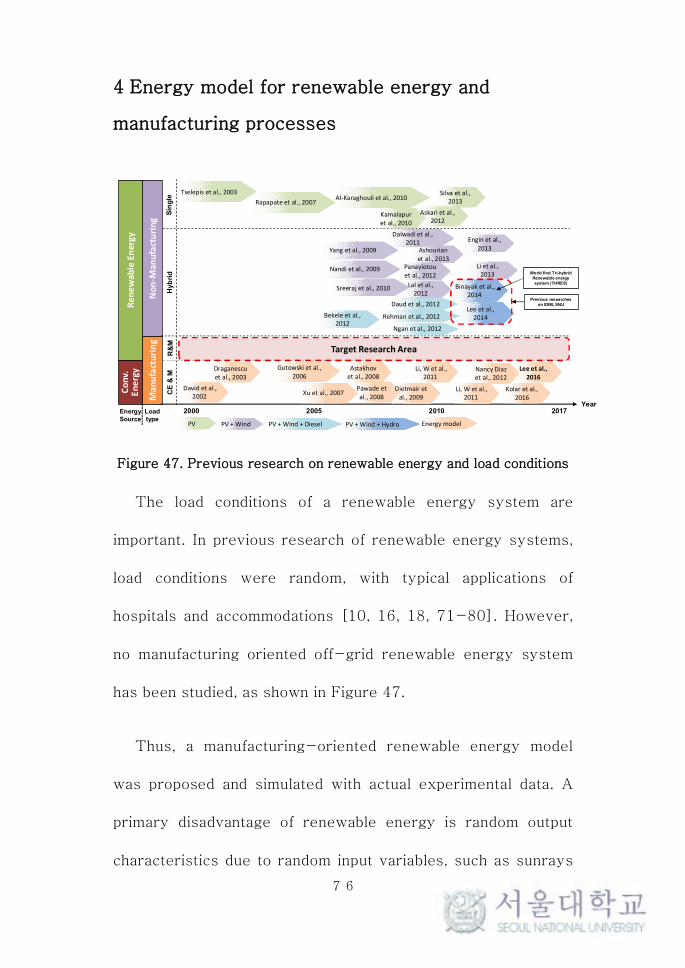
Figure 47. Previous research on renewable energy and load conditions

The load conditions of a renewable energy system are

important. In previous research of renewable energy systems,

load conditions were random, with typical applications of

hospitals and accommodations [10, 16, 18, 71-80]. However,

no manufacturing oriented off-grid renewable energy system

has been studied, as shown in Figure 47.

Thus, a manufacturing-oriented renewable energy model

was proposed and simulated with actual experimental data. A

primary disadvantage of renewable energy is random output

characteristics due to random input variables, such as sunrays

PV PV + Wind PV + Wind + Diesel Energy modelPV + Wind + Hydro

No

n-M

anu

fact

uri

ng

Ma

nu

fact

uri

ng

Loadtype

Sin

gle

CE

& M

Hyb

rid

EnergySource

Re

ne

wab

le E

ner

gyC

on

v.E

ne

rgy

Year

David et al., 2002

2000 2005 2010 2017

Target Research Area

Draganescuet al., 2003

Gutowski et al., 2006

Xu et al., 2007

Astakhovet al., 2008

Pawade et al., 2008

Nancy Diaz et al., 2012

Li, W et al., 2011

Dietmair et al., 2009

Li, W et al., 2011

Lee et al., 2016

Kolar et al., 2016

Tselepis et al., 2003

Kamalapuret al., 2010

Al-Karaghouli et al., 2010Rapapate et al., 2007

Askari et al., 2012

Silva et al., 2013

Dalwadi et al., 2011

Ashourian et al., 2013

Panayiotou et al., 2012

Yang et al., 2009

Nandi et al., 2009

Lal et al., 2012

Sreeraj et al., 2010

Engin et al., 2013

Li et al., 2013

Daud et al., 2012

Ngan et al., 2012

Rehman et al., 2012Bekele et al., 2012

Binayak et al., 2014

Lee et al., 2014

World first Tri-hybrid Renewable energy system (THRES)

R&

M

Previous researches on IDIM, SNU

７７

and wind speed, so a manufacturing-oriented model was

proposed and used for estimating not only the failure rate but

also the scale effect of a renewable energy plant for operating

manufacturing facilities.

4.1 Overview

Mathematical models of renewable energy sources and

manufacturing energy consumption were investigated and

implemented. Each of the equations was implemented in Matlab

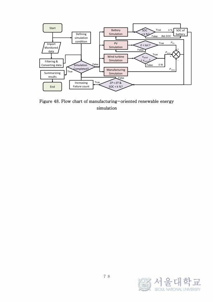
to simulate operating conditions. An overall simulation flow

chart is shown in Figure 48. The main purpose of a

manufacturing-oriented renewable energy simulation is to

estimate the stability of a renewable energy system with

manufacturing processes and provide scale effects of renewable

energy systems. In this research, the target components of a

renewable system include PV arrays, wind turbines, and a

battery bank. Input variables are monitored by an off-grid

monitoring platform.

７８

Figure 48. Flow chart of manufacturing-oriented renewable energy

simulation

Start

Filtering & Converting data

Import Monitored

data

Definingsimulation condition

Battery Simulation

PVSimulation

Wind turbineSimulation

ManufacturingSimulation

SOC of battery

E < tol.?

SOC < k %?

k %True

False

True

False

vwind< vcut in?

ΣP < 0? &SOC < k %?

True

False 0 W

Pwind

PPV

Bat.SOC

Pmanu

+

+

-

IncreasingFailure count

True

False

SimulationCompleted?

Summarizingresults

False

True

End

７９

4.2 Assumptions of models

Before modeling a manufacturing-oriented renewable

energy system, three assumptions should be defined first. The

first assumption is energy conservation of renewable energy

generation and manufacturing energy consumption. The amount

of energy generated from renewable energy sources is equal to

the sum of stored energy in batteries and energy consumption

for the load. The main controller and inverter consume little

amounts of energy and the battery has self-discharge

characteristics. Additionally, wires also consume a small

amount of energy when the current flows. However, the amount

of energy consumed by these components is relatively low such

that the energy losses from the controller, inverter, and wires

are negligible.

The second assumption is that there is no degradation effect

in short-term operation. There are several degradation models

for renewable energy systems. Although there is a degradation

effect on each component, process stability in a manufacturing

system is crucial so that monitoring and predicting failure

within a week is a sufficient period of time. Additionally, the

８０

purpose of this research is an instantaneous stability estimation

for a manufacturing-oriented model such that degradation

factors are negligible.

The third assumption is that the battery bank is fully

charged in the first state of operation. The SOC of the battery

bank is calculated by integrating the current flow of the battery.

Thus, there should be integrating constants for the initial

condition of the battery. Therefore, the battery is fully charged

in the first state of operation and for verification of modeling

results, the recharging period was at least 3 days and collecting

data and determining the fully charged battery for the test bed.

８１

4.3 Generalized load condition

Figure 49. Schematics of generalized load condition

To calculate various types of load conditions, Kirchhoff’s

rule was implemented on the power consumption side. Figure

49 shows Kirchhoff’s rules for various conditions for this

research. Even for an AC load condition with resistive and

inductive loads, the load condition can be estimated as the

summation of individual loads.

=

Load #1

Load #2

Load #n

…

Kirchhoff's rules

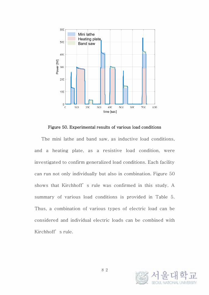
８２

Figure 50. Experimental results of various load conditions

The mini lathe and band saw, as inductive load conditions,

and a heating plate, as a resistive load condition, were

investigated to confirm generalized load conditions. Each facility

can run not only individually but also in combination. Figure 50

shows that Kirchhoff’s rule was confirmed in this study. A

summary of various load conditions is provided in Table 5.

Thus, a combination of various types of electric load can be

considered and individual electric loads can be combined with

Kirchhoff’s rule.

Mini latheHeating plateBand saw

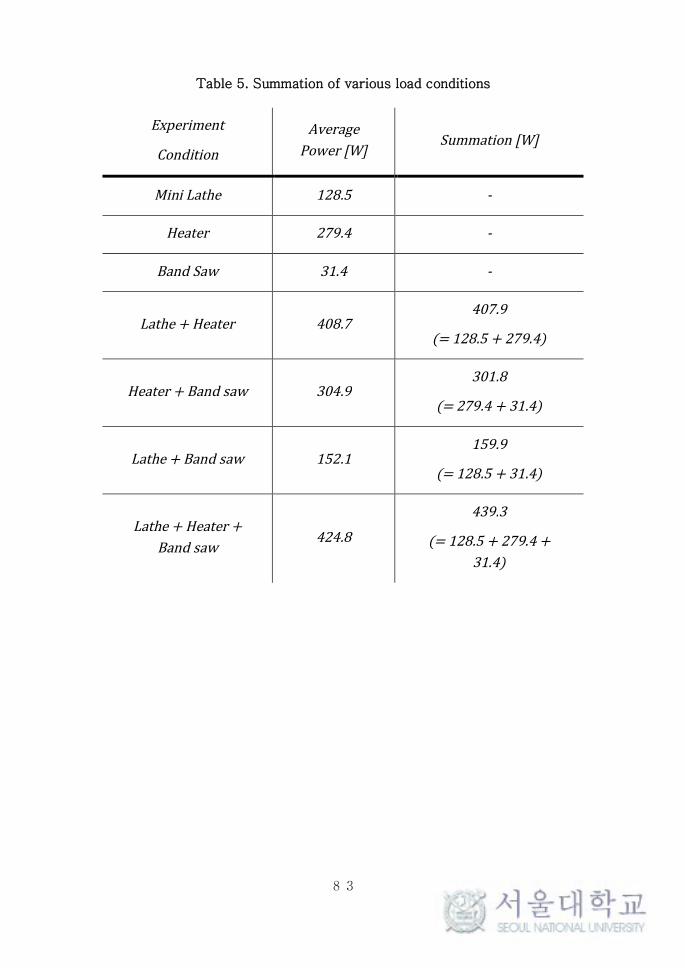
８３

Table 5. Summation of various load conditions

Experiment

Condition

Average

Power [W]Summation[W]

MiniLathe 128.5 -

Heater 279.4 -

BandSaw 31.4 -

Lathe +Heater 408.7407.9

(= 128.5 + 279.4)

Heater+ Bandsaw 304.9301.8

(= 279.4 + 31.4)

Lathe+Bandsaw 152.1159.9

(= 128.5 + 31.4)

Lathe+Heater+

Bandsaw424.8

439.3

(= 128.5 + 279.4 +

31.4)

８４

4.4 Test bed for model

An off-grid renewable energy test bed was installed at SNU,

Seoul. In total, eight PV arrays and a 400-W wind turbine were

installed (Figure 51). An off-grid monitoring platform was also

installed at the test bed. Hardware for the test bed differed

from the monitoring hardware in Nepal because different

numbers of sensors were applied in this case (Figure 52).

Figure 51. Off-grid renewable energy testbed in SNU

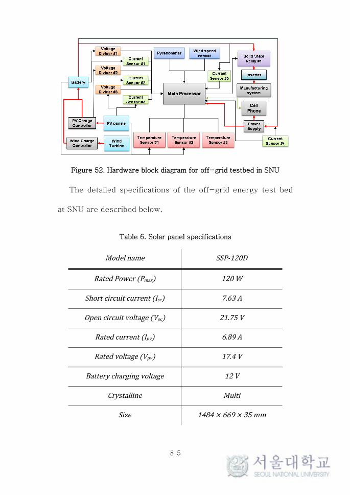
８５

Figure 52. Hardware block diagram for off-grid testbed in SNU

The detailed specifications of the off-grid energy test bed

at SNU are described below.

Table 6. Solar panel specifications

Modelname SSP-120D

RatedPower(Pmax) 120W

Shortcircuitcurrent(Isc) 7.63A

Opencircuitvoltage (Voc) 21.75 V

Ratedcurrent (Ipv) 6.89A

Ratedvoltage (Vpv) 17.4V

Batterychargingvoltage 12V

Crystalline Multi

Size 1484× 669× 35mm

８６

８７

Table 7. MPPT solar charge controller specifications

Modelname Tracer-4215BN

Ratedvoltage 12/24V(Autowork)

Chargealgorithm MaximumPowerPointTracking

Ratedchargecurrent 40A

Maximumbattery voltage 32 V

MaximumPVinputvoltage 150VDC

MaximumPVinputpower 520W(12 V)/1040W (24V)

Self-consumption ≤ 50 mA(12 V)/ ≤ 27 mA(24 V)

Table 8. Wind turbine specifications

Modelname FA24V-400

RatedPower 400W

Rotor diameter 1.2m

Start-upwindspeed 2m/s

Yawmode Fixed-wing

Ratedvoltage (V) 24 V

Shellmaterial Die-cast aluminum

Bladematerial High-strengthnyloncomposite

Motortype Single-phasepermanentmagnetDC

generator

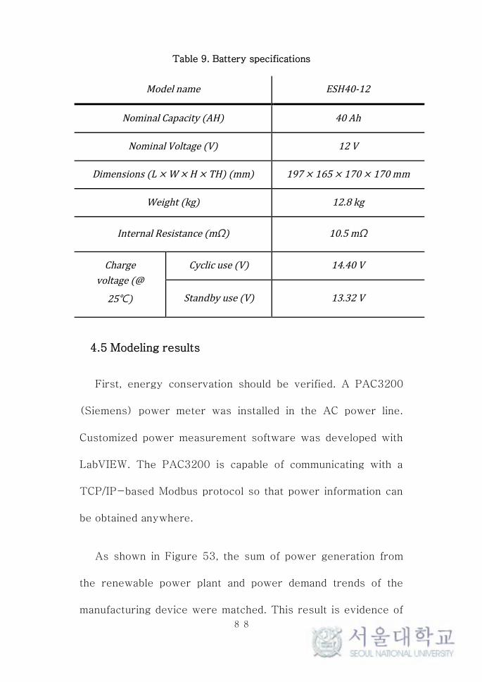
８８

Table 9. Battery specifications

Modelname ESH40-12

NominalCapacity(AH) 40Ah

NominalVoltage(V) 12V

Dimensions(L× W× H× TH)(mm) 197× 165× 170× 170mm

Weight(kg) 12.8kg

InternalResistance(mΩ) 10.5mΩ

Charge

voltage(@

25)

Cyclicuse(V) 14.40V

Standbyuse(V) 13.32V

4.5 Modeling results

First, energy conservation should be verified. A PAC3200

(Siemens) power meter was installed in the AC power line.

Customized power measurement software was developed with

LabVIEW. The PAC3200 is capable of communicating with a

TCP/IP-based Modbus protocol so that power information can

be obtained anywhere.

As shown in Figure 53, the sum of power generation from

the renewable power plant and power demand trends of the

manufacturing device were matched. This result is evidence of

８９

energy conservation in the system.

Failure of the off-grid system was detected at 22 V in the

battery bank (Figure 54). The SOC was also calculated for the

battery model with current measurement data (Figure 57).

Thus, criteria for failure modes can be estimated with the SOC

of the battery bank.

Figure 53. Power trends of direct measurement and modeled results

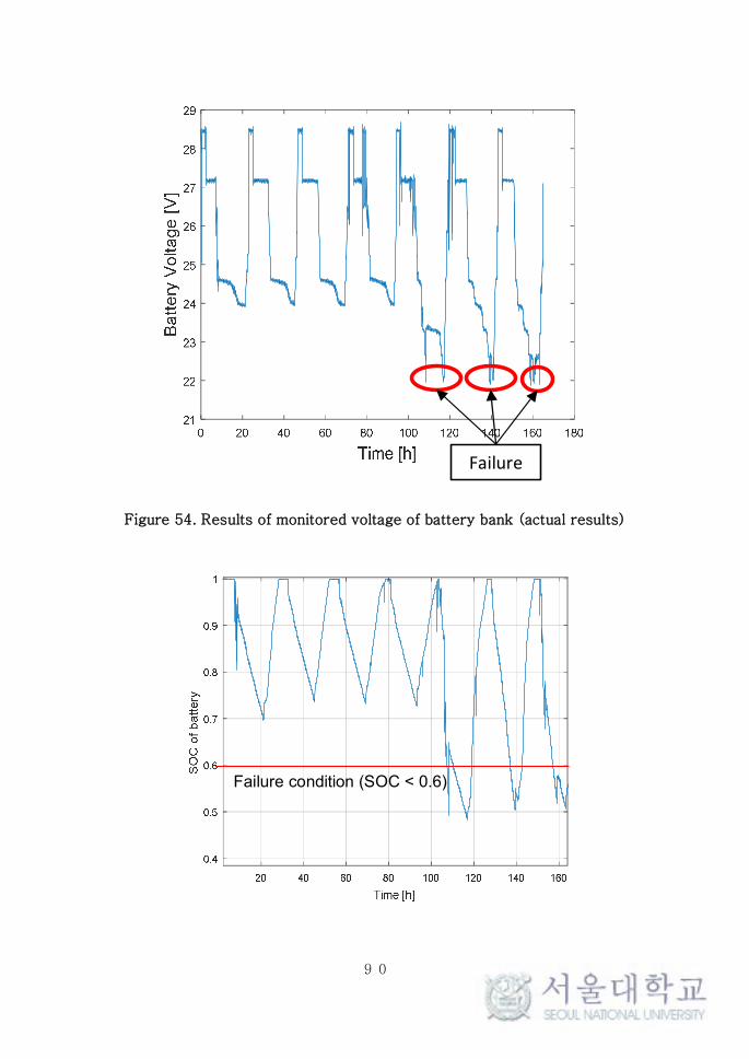
９０

Figure 54. Results of monitored voltage of battery bank (actual results)

Failure

Failure condition (SOC < 0.6)

９１

Figure 55. Results of monitored SOC of battery bank (actual results)

4.5.1 Case study 1: 3D Printer

To measure stability of the off-grid renewable energy

system with manufacturing processes, a simple target specimen

was designed (Figure 56). The target manufacturing process is

a three dimensional (3D) printer (3Dwox DP200, Shindoh

Corp.). Detailed specifications of the 3D printer are described

in Table 10.

NC code was automatically generated by the provided CAM

software. To obtain operating conditions, interpreter software

was developed. Results of the interpretation of the NC code for

position information are shown in Figure 57.

Figure 56. Dimensions of the test specimen

20 mm

10 mm

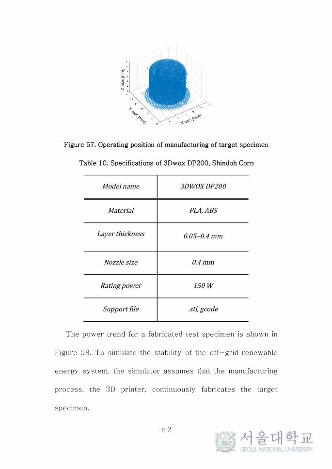
９２

Figure 57. Operating position of manufacturing of target specimen

Table 10. Specifications of 3Dwox DP200, Shindoh Corp

Modelname 3DWOXDP200

Material PLA,ABS

Layerthickness 0.05–0.4mm

Nozzlesize 0.4mm

Ratingpower 150W

Supportfile .stl,gcode

The power trend for a fabricated test specimen is shown in

Figure 58. To simulate the stability of the off-grid renewable

energy system, the simulator assumes that the manufacturing

process, the 3D printer, continuously fabricates the target

specimen.

Z a

xis

[mm

]

９３

Figure 58. Power trends of a three dimensional (3D) printer to

fabricate a target specimen

Figure 59. SOC result with six PV arrays and two wind turbines

Process time = 20 min

Total energy consumption = 50.624 Wh

Failure condition (SOC < 0.6)

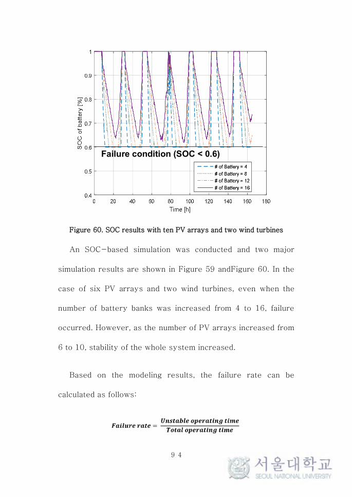
９４

Figure 60. SOC results with ten PV arrays and two wind turbines

An SOC-based simulation was conducted and two major

simulation results are shown in Figure 59 andFigure 60. In the

case of six PV arrays and two wind turbines, even when the

number of battery banks was increased from 4 to 16, failure

occurred. However, as the number of PV arrays increased from

6 to 10, stability of the whole system increased.

Based on the modeling results, the failure rate can be

calculated as follows:

Failure condition (SOC < 0.6)

９５

Overall stability of the off-grid manufacturing system is

correlated with the incoming power source (solar irradiation,

wind speed), scale of the renewable energy system, and

capabilities of the battery bank. Wind speed varies with the

installation location of the wind turbines. Thus, wind speed is

varied by multiplying wind speed data to observe the effects of

natural energy sources.

The failure rate indicates the stability of the whole system;

if the failure rate reaches 0, it means it exhibits stable around-

the-clock operating conditions for the manufacturing process.

However, if the manufacturing process is fixed, an appropriate

scale of the renewable energy system is present, and if the

manufacturing parameters are controlled, the surface of the

failure rate would approach 0, so that the minimum

requirements for the renewable energy system scale decrease,

which means a minimal-scale renewable energy system could

be used with manufacturing facilities.

９６

Figure 61. Surface of failure rate vs. scale of renewable energy system

(@ 1 × vwind)

Figure 62. Surface of failure rate vs. scale of renewable energy system

(@ 3 × vwind)

９７

Figure 63. Surface of failure rate vs. scale of renewable energy system

(@ 5 × vwind)

With the modeling results, a manufacturing-oriented off-

grid system was designed (960 W of a total of eight PV arrays,

two in series, four in parallel; 320 Ah at 24 V for a total of eight

batteries, two in series and four in parallel; and a 400-W wind

turbine), installed, and operated with the same manufacturing

process from April 20– 26. Energy conservation was verified

with direct measurement data and modeled (Figure 64).

With the modeling results above, the estimated failure rate

of the redesigned system was 0.033 (Figure 65). Operating

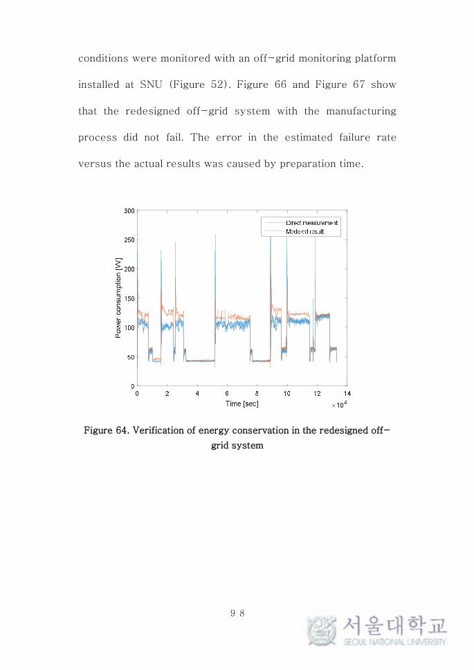
９８

conditions were monitored with an off-grid monitoring platform

installed at SNU (Figure 52). Figure 66 and Figure 67 show

that the redesigned off-grid system with the manufacturing

process did not fail. The error in the estimated failure rate

versus the actual results was caused by preparation time.

Figure 64. Verification of energy conservation in the redesigned off-

grid system

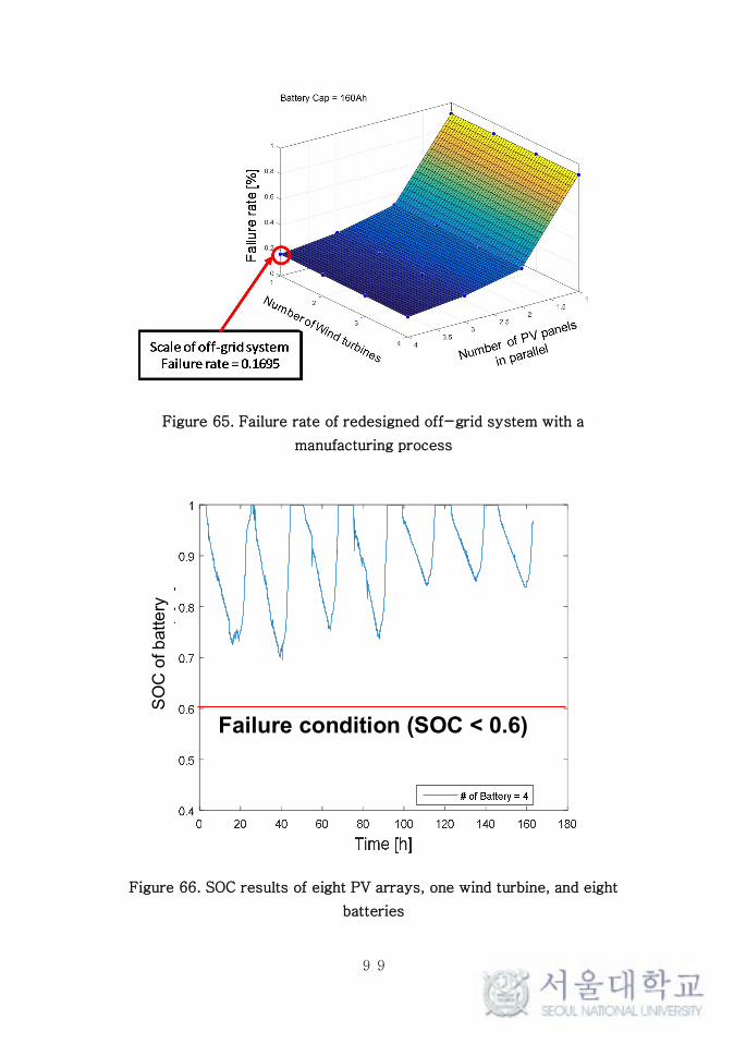
９９

Figure 65. Failure rate of redesigned off-grid system with a

manufacturing process

Figure 66. SOC results of eight PV arrays, one wind turbine, and eight

batteries

Failure condition (SOC < 0.6)

SO

C o

f b

atte

ry

１００

Figure 67. Results of battery bank voltage (actual data)

4.5.2 Case study 2: Lathe

Similar to the first case, the lathe is the second case for a

larger-scale manufacturing system. The target lathe machine is

a NL2000SY and its power profile was simulated with the

time-wise simulator proposed in Chapter 0. The manufacturing

procedure is described in Figure 68.

Failure under 22 V

１０１

Figure 68. Process procedure for case study: the lathe

The failure rate surface was calculated with the simulation

results. Because of the scale of the manufacturing process, the

minimum requirement scale for the renewable energy system is

much larger than in case 1. As shown in Figure 69, the capacity

of the battery was 8,000 Ah with 200 PV arrays for the

renewable energy system to reach a failure rate of almost 0.

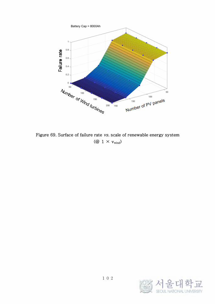
１０２

Figure 69. Surface of failure rate vs. scale of renewable energy system

(@ 1 × vwind)

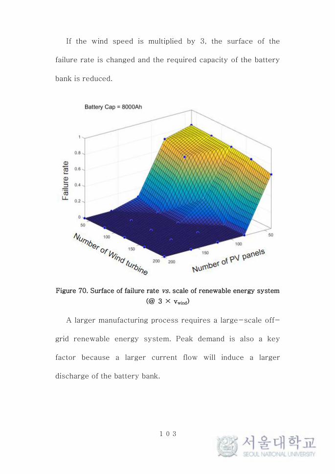
１０３

If the wind speed is multiplied by 3, the surface of the

failure rate is changed and the required capacity of the battery

bank is reduced.

Figure 70. Surface of failure rate vs. scale of renewable energy system

(@ 3 × vwind)

A larger manufacturing process requires a large-scale off-

grid renewable energy system. Peak demand is also a key

factor because a larger current flow will induce a larger

discharge of the battery bank.

１０４

4.5.3 Case study 3: Band saw

A band saw is a simple manufacturing tool that is capable of

fabricating simple two dimensional (2D) parts. An off-grid

renewable energy system would typically be installed in a rural

area of a developing country so a simple manufacturing facility

should be considered. Thus, the band saw is a good candidate

for analysis.

Nine repeat cuts of a 1-mm thick acrylic plate were

performed with an off-grid renewable system (Figure 71). The

simulation result showed that a 240-W PV array, 400-W wind

turbine, and a 120 Ah battery bank system would be required

for continuous cutting processes with the band saw (Figure 72).

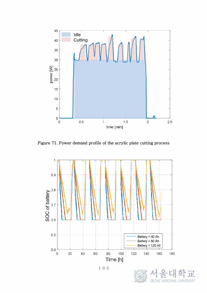
１０５

Figure 71. Power demand profile of the acrylic plate cutting process

IdleCutting

SO

C o

f b

atte

ry

１０６

Figure 72. Simulation results of an off-grid renewable energy system

with a band saw

１０７

4.5.4 Case study 4: Vaccine carrier

A vaccine carrier can have a large impact in developing

countries. However, some countries do not have the

infrastructure for electricity so an active-type vaccine carrier

was developed as a practical example of an off-grid renewable

system. A vaccine carrier is a good example for estimating the

stability of an off-grid energy system.

Recently, cold-chain procedures were proposed for

delivering vaccines farther than a single vaccine carrier. Cold-

chain requires stable electricity so that the proposed model can

estimate the stability of the whole system with multiple vaccine

carriers. The vaccine carrier consists of the cooling part, the

Peltier module. In this research, the power demands of a single

Peltier-type vaccine carrier were measured and a simulation

method was used to estimate the stability of an off-grid system

with a vaccine carrier.

Figure 73 shows the power demands of the vaccine carrier

in two states: cooling on and off. A stable-size off-grid

renewable energy system for cold chain storage in rural areas

for vaccine carriers requires a 360-W PV array, a 400-W

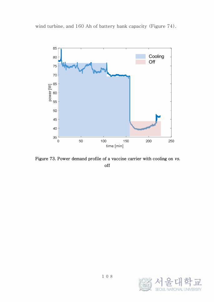
１０８

wind turbine, and 160 Ah of battery bank capacity (Figure 74).

Figure 73. Power demand profile of a vaccine carrier with cooling on vs.

off

po

we

r [W

]

CoolingOff

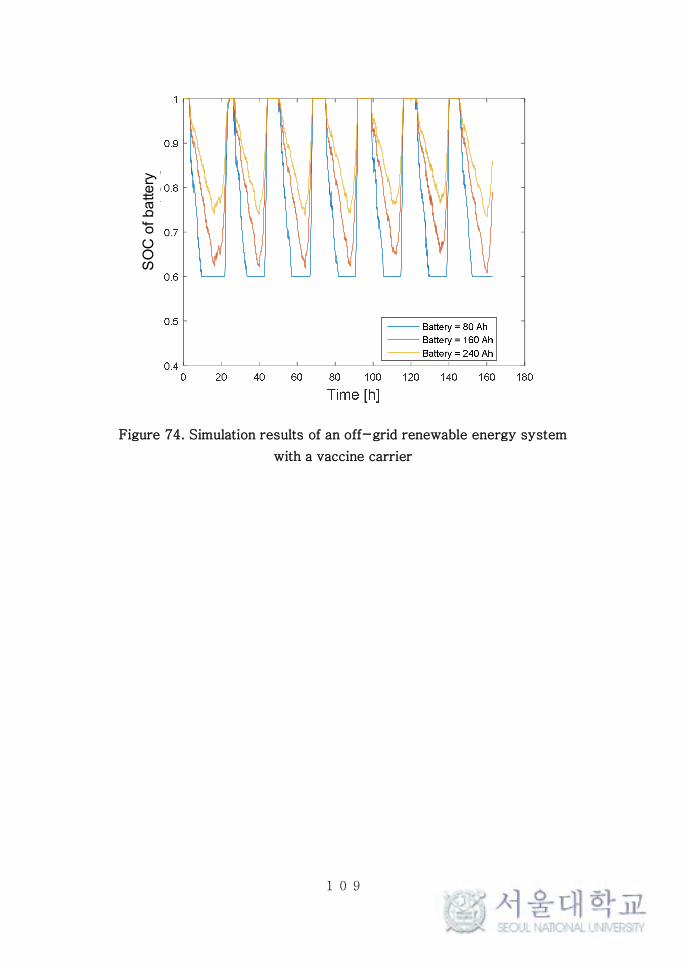
１０９

Figure 74. Simulation results of an off-grid renewable energy system

with a vaccine carrier

SO

C o

f b

atte

ry

１１０

4.5.5 Comparison with other models

Monte-Carlo-based analyses are widely used in the design

of off-grid renewable energy plants for rural areas. The major

merit of such a statistical analysis is that the modeled results

propose the appropriate scale for various types of load

conditions. However, design results based on statistical

methods tend to overdesign an off-grid system.

The Monte-Carlo method examines several samples and

generates random input variables. An even load condition is

generated randomly and power generation can be calculated

simultaneously. Accommodating load conditions can be modeled

with statistical methods so that the Monte-Carlo simulation fits

in randomized load conditions [81].

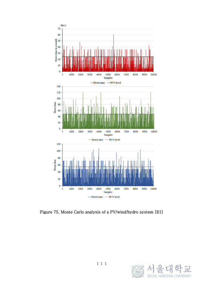
１１１

Figure 75. Monte Carlo analysis of a PV/wind/hydro system [81]

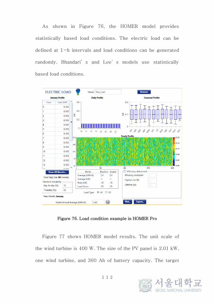
１１２

As shown in Figure 76, the HOMER model provides

statistically based load conditions. The electric load can be

defined at 1-h intervals and load conditions can be generated

randomly. Bhandari’s and Lee’s models use statistically

based load conditions.

Figure 76. Load condition example in HOMER Pro

Figure 77 shows HOMER model results. The unit scale of

the wind turbine is 400 W. The size of the PV panel is 2.01 kW,

one wind turbine, and 360 Ah of battery capacity. The target

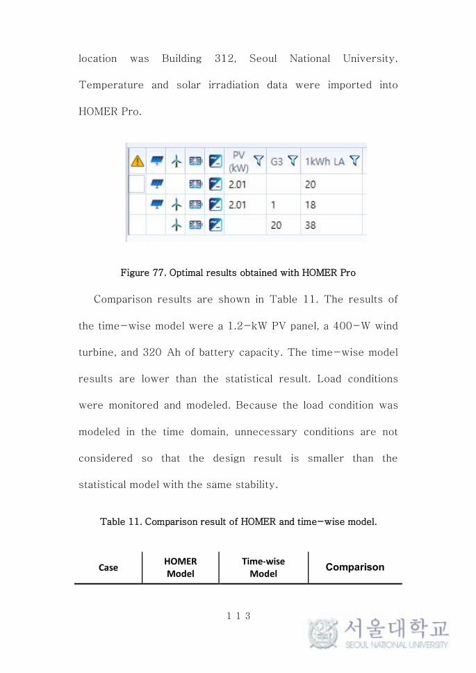
１１３

location was Building 312, Seoul National University.

Temperature and solar irradiation data were imported into

HOMER Pro.

Figure 77. Optimal results obtained with HOMER Pro

Comparison results are shown in Table 11. The results of

the time-wise model were a 1.2-kW PV panel, a 400-W wind

turbine, and 320 Ah of battery capacity. The time-wise model

results are lower than the statistical result. Load conditions

were monitored and modeled. Because the load condition was

modeled in the time domain, unnecessary conditions are not

considered so that the design result is smaller than the

statistical model with the same stability.

Table 11. Comparison result of HOMER and time-wise model.

CaseHOMERModel

Time-wiseModel

Comparison

１１４

PV 2,010 W 1,200 W-500 W[-40.3%]

Wind 400 W 400 W 0 W

Battery 360 Ah 320 Ah-40 Ah

[-12.5%]

4.6 Summary

A manufacturing-oriented simulation method was introduced

and the simulation was compared with actual monitored data. A

data set was provided to the off-grid monitoring platform and

the stability of the whole system was calculated. Two

manufacturing processes were investigated as case studies and

failure rate surfaces were calculated. Moreover, a statistical

model widely used in off-grid systems is used to perform a

comparison with the modeling results.

Various load conditions for the off-grid system were

analyzed with the proposed simulation method. In total, four

cases of load conditions were considered: a 3D printer, a

large-scale lathe, a band saw, and a vaccine carrier. Four

practical cases of load conditions were measured and simulated

and the stable system size for each condition was obtained.

１１５

Furthermore, the proposed model was compared with a

statistical model, the HOMER model, to show that the time-

wise simulation method has value in designing an off-grid

system. With the same rating load conditions in both models,

the proposed model obtained a smaller scale off-grid system.

Moreover, peak demand could be considerable within a few

seconds.

１１６

5 Conclusions

Emerging problems with energy generating sources have

grown since the era of the industrial revolution. Global warming

has been realized as a problem and the ‘climate crisis’ has

accelerated. Furthermore, in developing countries, renewable

energy systems are used widely and the energy consumption

ratio of renewable energy has increased. From the point of view

of manufacturing industries, the largest portion of energy

consumption in South Korea, renewable energy is not attractive

because of the unstable characteristics of energy sources (e.g.,

solar radiation, wind speed). Thus, monitoring of renewable

energy systems is crucial in predicting their stability.

For developing countries, real-time off-grid renewable

energy monitoring systems for rural areas have not been

developed. As such, an SMS-based real-time monitoring

platform was developed and installed in a developing country,

Nepal.

To further investigate the stability of renewable energy

systems, a manufacturing-oriented energy system was

１１７

introduced and a simulation method was developed. An off-grid

renewable energy test bed was installed in SNU, Seoul, and two

manufacturing cases were investigated. From small to large

scale manufacturing processes, an SOC-based simulation

method was implemented and the failure rate with a monitored

data set and manufacturing energy consumption simulator were

calculated. Finally, a scale effect of the renewable energy

system could be obtained based on manufacturing processes

with an off-grid monitoring platform and could provide stability

of the renewable energy system with regard to the

manufacturing processes examined.

１１８

Appendix

Monitoring system for a renewable energy system

On-grid energy monitoring systems are widely used

because fully functioning infrastructures have already been

implemented [82-85]. Thus, a monitoring system with an on-

grid system uses high-speed communication protocols. Due to

the large bandwidth in communication capability, a large data

set can be transmitted and analyzed with high-performance

hardware. A high-speed data acquisition rate supports a high

level of stability in controlling a target system [86, 87].

１１９

Figure 78. Issues in an off-grid renewable energy system

In the case of an off-grid renewable energy monitoring

system, the impact is much larger than with an on-grid system.

Off-grid systems are commonly installed in rural areas so the

infrastructure is not necessarily fully functional. Communication

capabilities are significantly lower and there are typically no

trained engineers working in rural areas. If the whole system

malfunctions, it can take several months to fix the problem.

Sometimes, malfunctioning is not even reported for a few

weeks.

Several off-grid type power systems have been installed in

several different countries. Stand-alone PV power systems [24,

88-93], PV/wind power systems [15, 16, 18, 63, 74, 94-98],

and PV/wind/diesel power systems [75, 77, 99-101] have

been investigated. Akikur et al. surveyed over 30 different off-

grid rural systems [102]. The scale of an off-grid rural energy

system varies with the demand load scale. Some of them have

monitoring systems locally (Table 12), although an off-grid

system is typically installed in a rural area and a remote

monitoring system is not installed even with a large-scale

energy system.

１２０

１２１

Table 12. Previous research of off-grid renewable energy systems

Study/Project location

Total annual load Monitoring Reference

Vadodara, India 1825 kWh/year - (Dalwadi et al. 2011) [94]

Juara village, Tioman island, Malaysia

181.04 MWh/year Local(Ashourian et al. 2013)

[95]

Two different sites: 1. Nice, France;2. Nicosia, Cyprus

8760 kWh/year -(Panayiotou, Kalogirou, and Tassou 2012) [96]

Dalajia Island in China 13.14 MWh/year -(Yang, Wei, and Chengzhi

2009) [97]

Sitakuda, Bangladesh 61,685 kWh/year -(Nandi and Ghosh 2009)

[18]

Naboualu Vanua Levu Island, Fiji

360.985 MWh/year Local (Lal and Raturi 2012) [15]

Sukhalai, Hoshangabad, Madhya Pradesh, India

15,768 kWh/year Local(Sreeraj, Chatterjee, and

Bandyopadhyay 2010) [74]

Turkey 1142 kWh/year - (Engin 2013) [63]

Patenga, Chittagong, Bangladesh

58.4 MWh/year Local(Nandi and Ghosh 2010)

[98]

Urumqi, China 4.015 MWh/year Local (Li et al. 2013) [16]

Some researchers have investigated cell phone-based data

collecting technology in rural areas of Ghana and controlling

simple hand pumps in Zambia [103]. As shown in the results of

hand pump monitoring, even a simple monitoring method can

have a huge impact.

１２２

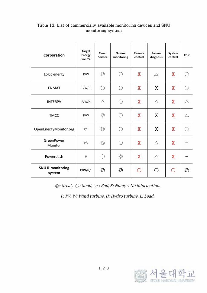
１２３

Table 13. List of commercially available monitoring devices and SNU

monitoring system

CorporationTarget Energy Source

Cloud Service

On-line monitoring

Remote control

Failure diagnosis

System control

Cost

Logic energy P/W X X

ENMAT P/W/B X X X

INTERPV P/W/H X X

TMCC P/W X X X

OpenEnergyMonitor.org P/L X X X

GreenPowerMonitor

P/L X X -

Powerdash P X X -

SNU R-monitoring system

P/W/H/L

: Great, : Good, : Bad,X: None,-:No information.

P: PV,W: Windturbine,H: Hydroturbine,L: Load.

１２４

Issues in data transmission via telecommunication methods

The major issues regarding data transmission via

telecommunication include the communication frequencies for

mobile phones. In this research, an off-grid renewable energy

system was installed at Thingan and Kolkhop, in Nepal. There

are three major telecommunications companies in Nepal: Nepal

telecom, Ncell, and Smart telecom. The location of the target

system is highlighted with a red dot in Figure 79.

Communication coverage and frequencies were provided by

each telecommunication service company. Nepal telecom

provided the widest range of frequencies, followed by Ncell.

Table 14. Communication frequencies in Nepal

Technology Frequency Operator

LTE(4G) 1800MHz NepalTelecom

GSM900MHz/1800

MHz

NepalTelecom,Ncell,

SmartTelecom

CDMA800MHz/1900

MHzUTL,Nepal Telecom

WCDMA(3G) 2100MHz NepalTelecom,Ncell

WiMAX 2300MHz NepalTelecom

１２５

Figure 79. Communication coverage in Nepal

The cost of data transmission with SMS and multimedia

messaging service (MMS) is a major issue for a monitoring

system. International transmission costs of SMS are quite high

so the data-transmitting interval is important. Table 15 shows

detailed cost information for SMS from Nepal to South Korea.

Table 15. Detailed information of SMS cost

Item Quantity

SMScostfromNepaltoKorea ₹6

MMScostfromNepaltoKorea ₹12

Max.DatalengthofSMS 80

Max.DatalengthofMMS 1,000

Currency(￦/₹) 17.61

From Table 15, a cost estimation surface was obtained to

estimate the relationship between data interval and data length

versus data transmitting costs per month. The data interval is

１２６

directly related to the cost of SMS and data length indicates the

limitations of the data transmitting form.

Figure 80. Cost estimate of MMS per month

Figure 81. Cost estimate of SMS per month

１２７

Issues regarding bidirectional control

Bidirectional control is necessary for controlling an off-grid

power system in a rural area. Once the telecommunication line

is confirmed, bidirectional communication can be confirmed too.

Because of the different interfaces between Arduino- and

Android-based smart phones, customized data trimming and

interrupting should be implemented in the monitoring platform.

Thus, a serial communication interrupt was implemented so that

a control solid state relay (SSR) was possible as soon as a

control message was acquired.

Summary

Previously, there have been monitoring systems for off-grid

renewable energy systems in rural areas. However, none of

them could transmit data back from the rural area. Because of

the lack of telecommunication capabilities in these areas, a

primitive telecommunication service was investigated to

overcome difficulties in the transmission of data from rural

areas. A target off-grid energy system was installed in

１２８

Thingan, Nepal, and telecommunication capabilities were

investigated and we estimated the cost of data transfer. Finally,

telecommunication capabilities were confirmed and the

capabilities of the monitoring device were defined.

Objectives

Based on previous research and commercially available

devices, it is worth developing a monitoring platform capable of

transmitting data in real time from a rural area. An off-grid

system should be monitored in real time and the stability of the

target system should be estimated.

Thus, the research objectives were 1) to develop an off-

grid monitoring platform, 2) develop a renewable energy model

for estimating the stability of the off-grid energy system, and 3)

develop a manufacturing-oriented model and verify the

stability of the off-grid energy system with some

manufacturing process examples.

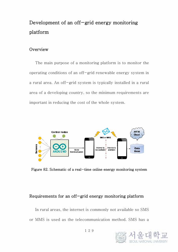
１２９

Development of an off-grid energy monitoring

platform

Overview

The main purpose of a monitoring platform is to monitor the

operating conditions of an off-grid renewable energy system in

a rural area. An off-grid system is typically installed in a rural

area of a developing country, so the minimum requirements are

important in reducing the cost of the whole system.

Figure 82. Schematic of a real-time online energy monitoring system

Requirements for an off-grid energy monitoring platform

In rural areas, the internet is commonly not available so SMS

or MMS is used as the telecommunication method. SMS has a

１３０

short data length per message. However, a wide communication

range is possible and once communication capabilities are

confirmed, bi-directional communication is possible.

Sensor nodes can be fabricated at low cost. Sensors for an

off-grid system should be compact and rigid even under harsh

environmental conditions. Commercially available sensors are

rigid and accurate but often too expensive to install in rural

areas in developing countries. If sensor breakdown occurs, the

cost of maintenance can increase dramatically.

The core processor also requires high stability at low cost.

Arduino is a strong candidate; however, any type of embedded

system could be implemented. A customized Real-Time OS

(RTOS) can be implemented to accurately control sensor nodes

and the data transmission interval.

Finally, several application capabilities are necessary for the

end-user. Thus, Web DB and a cloud service were connected

to the monitoring platform. As one example, ARTIK Cloud was

used to monitor an off-grid system on a web page.

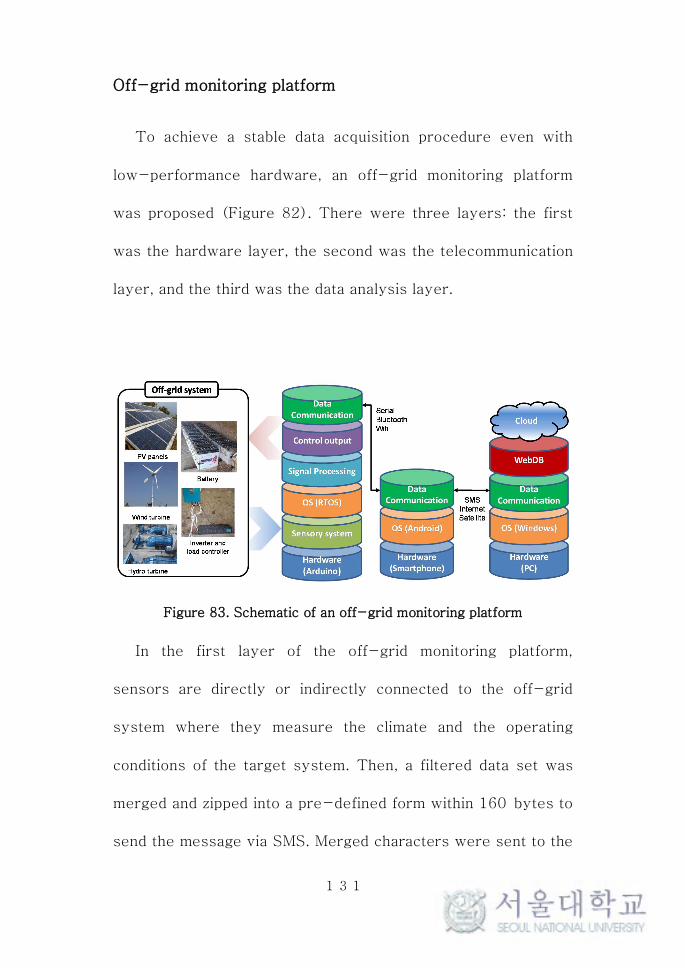
１３１

Off-grid monitoring platform

To achieve a stable data acquisition procedure even with

low-performance hardware, an off-grid monitoring platform

was proposed (Figure 82). There were three layers: the first

was the hardware layer, the second was the telecommunication

layer, and the third was the data analysis layer.

Figure 83. Schematic of an off-grid monitoring platform

In the first layer of the off-grid monitoring platform,

sensors are directly or indirectly connected to the off-grid

system where they measure the climate and the operating

conditions of the target system. Then, a filtered data set was

merged and zipped into a pre-defined form within 160 bytes to

send the message via SMS. Merged characters were sent to the

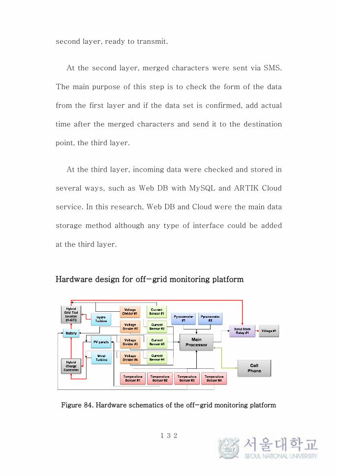
１３２

second layer, ready to transmit.

At the second layer, merged characters were sent via SMS.

The main purpose of this step is to check the form of the data

from the first layer and if the data set is confirmed, add actual

time after the merged characters and send it to the destination

point, the third layer.

At the third layer, incoming data were checked and stored in

several ways, such as Web DB with MySQL and ARTIK Cloud

service. In this research, Web DB and Cloud were the main data

storage method although any type of interface could be added

at the third layer.

Hardware design for off-grid monitoring platform

Figure 84. Hardware schematics of the off-grid monitoring platform

１３３

Main processor

The main processor of the monitoring system was Arduino

Mega. Arduino Mega is equipped with 10 bits, 16 channels of

ADC, and tens of digital I/Os. The processor was equipped with

serial communications and an internal timer and interrupt.

Sensors

To sense solar irradiation, a customized pyranometer was

fabricated and tested. SP-215 (Apogee Corp.) was used for

calibrating the sensor signal. The zenith angle is crucial for

calculating incident radiation from the sun so a sensor cap was

fabricated. A Teflon disk 2 mm thick was fabricated and used to

cover the top of the sensor cap (Figure 85). A PDB-C139

photodiode was used. Results of the calibrated sensor are

shown in Figure 86.

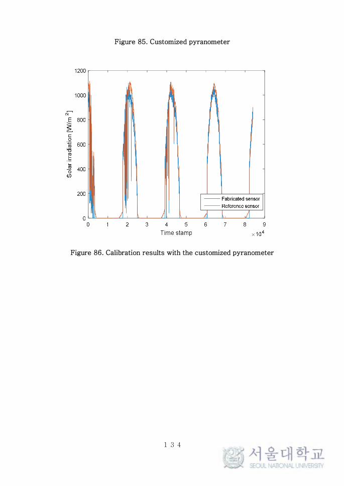
１３４

Figure 85. Customized pyranometer

Figure 86. Calibration results with the customized pyranometer

１３５

The temperature sensor was a TC1047AVNB (Microchip

Technology Inc.), which has temperature range of – 40 to

125°C with a high linear signal (Figure 87) [104].

Figure 87. Output curve of the temperature sensor [104]

A Hall effect-based ring-type current sensor (WCS1x00

series) was used to monitor current flow in the off-grid energy

system. The Hall effect-based sensor has high linearity

(Figure 88) [105].

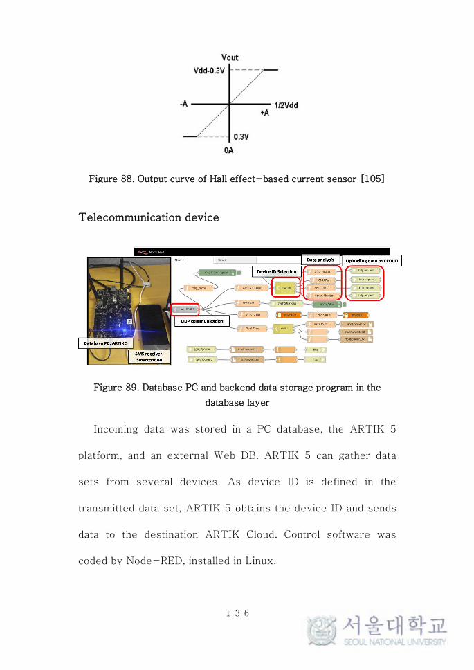
１３６

Figure 88. Output curve of Hall effect-based current sensor [105]

Telecommunication device

Figure 89. Database PC and backend data storage program in the

database layer

Incoming data was stored in a PC database, the ARTIK 5

platform, and an external Web DB. ARTIK 5 can gather data

sets from several devices. As device ID is defined in the

transmitted data set, ARTIK 5 obtains the device ID and sends

data to the destination ARTIK Cloud. Control software was

coded by Node-RED, installed in Linux.

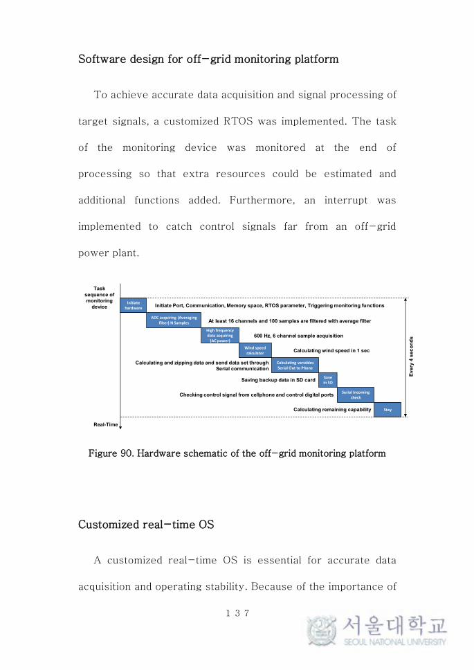
１３７

Software design for off-grid monitoring platform

To achieve accurate data acquisition and signal processing of

target signals, a customized RTOS was implemented. The task

of the monitoring device was monitored at the end of

processing so that extra resources could be estimated and

additional functions added. Furthermore, an interrupt was

implemented to catch control signals far from an off-grid

power plant.

Figure 90. Hardware schematic of the off-grid monitoring platform

Customized real-time OS

A customized real-time OS is essential for accurate data

acquisition and operating stability. Because of the importance of

Real-Time

Task sequence of monitoring

device

ADC acquiring (Averaging filter) N Samples

Calculating variablesSerial Out to Phone

Stay

Save in SD

Serial Incoming check

Wind speed calculator

High frequency data acquiring

(AC power)

Initiate hardware

Initiate Port, Communication, Memory space, RTOS parameter, Triggering monitoring functions

At least 16 channels and 100 samples are filtered with average filter

600 Hz, 6 channel sample acquisition

Calculating wind speed in 1 sec

Calculating and zipping data and send data set through Serial communication

Saving backup data in SD card

Checking control signal from cellphone and control digital ports

Calculating remaining capabilityE

ve

ry 4

se

co

nd

s

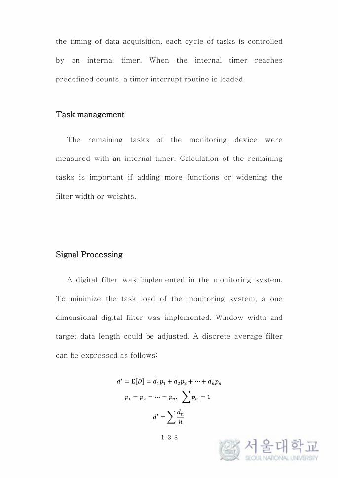
１３８

the timing of data acquisition, each cycle of tasks is controlled

by an internal timer. When the internal timer reaches

predefined counts, a timer interrupt routine is loaded.

Task management

The remaining tasks of the monitoring device were

measured with an internal timer. Calculation of the remaining

tasks is important if adding more functions or widening the

filter width or weights.

Signal Processing

A digital filter was implemented in the monitoring system.

To minimize the task load of the monitoring system, a one

dimensional digital filter was implemented. Window width and

target data length could be adjusted. A discrete average filter

can be expressed as follows:

= E[] = + +⋯+

= = ⋯ = , = 1

′ =

１３９

where D is the set of data, dn is the nth single data point of D,

d’ are filtered data, pn is the probability of each data point dn

as the weight of the discrete filter, and n is the length of the

data as the window width of the digital filter.

There are two different signal acquisition procedures. The

first is low-speed data measurement for DC signals and the

other is high-speed data measurement for AC signals.

Low-speed data measurement

The low-speed data measurement procedure is suitable for

temperature, DC voltage, DC current, solar irradiation, and any

type of DC signal. The low-speed data measurement procedure

acquires a data set with user-defined width and then a digital

filter was applied to reduce external noise.

High-speed data measurement

The high-speed data measurement procedure is suitable for

AC voltage, AC current, and any type of AC signal. Because of

the relatively high frequency of AC power (commonly 50/60

Hz), high-speed data measurement is at 600 Hz.

１４０

Development results

The most important function of the monitoring platform is

communication, so the first prototype was sent to Nepal on

January 24th. Two temperature sensors and two current

sensors were provided in the first version. Nepal Telecom

provided telecommunication services for transmitting SMS.

Figure 91 and Figure 92 show the installation results and

incoming SMSs from Nepal.

１４１

Figure 91. First test set up for data transmitting from Nepal to South

Korea

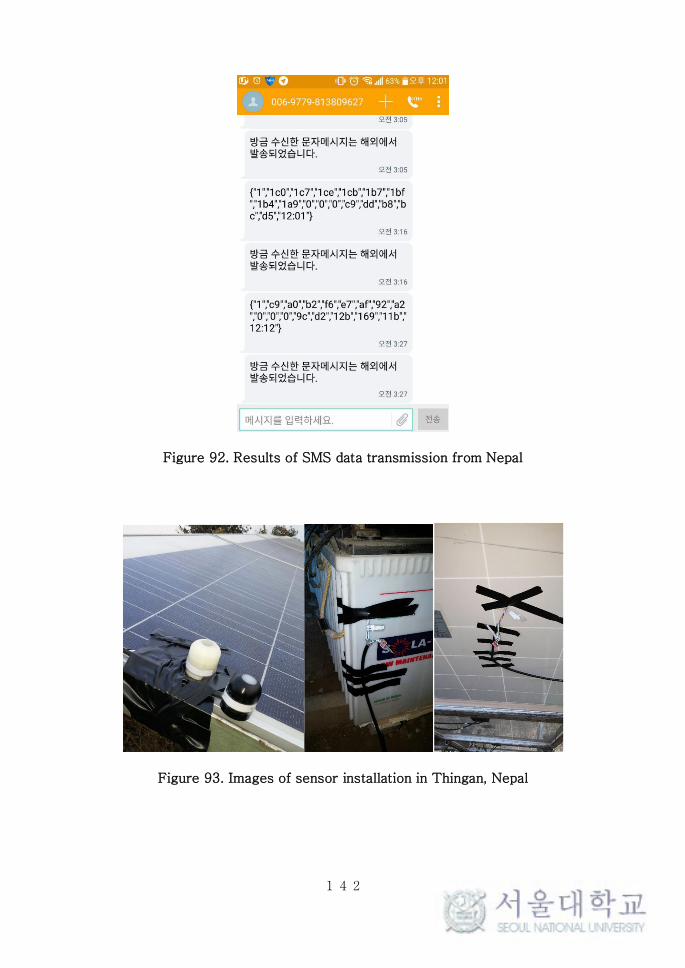
１４２

Figure 92. Results of SMS data transmission from Nepal

Figure 93. Images of sensor installation in Thingan, Nepal

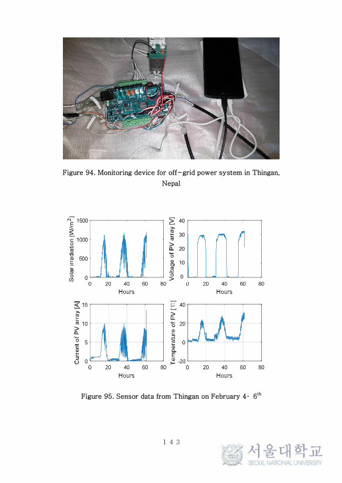
１４３

Figure 94. Monitoring device for off-grid power system in Thingan,

Nepal

Figure 95. Sensor data from Thingan on February 4– 6th

40

30

20

10

0

１４４

Development summary

For two sets of tests, the off-grid monitoring platform from

Nepal to South Korea was used. An off-grid monitoring system

was developed and applied to a renewable system in Thingan,

Nepal. Climate data and power data were acquired successfully

and data sets were transmitted via SMS. Controllability of the

monitoring platform was confirmed. A control signal was sent

from South Korea to Nepal via SMS and the monitoring platform

control SSR to turn on/off the load current.

１４５

6 Bibliography

[1] "GISTEMP Team, 2017: GISS Surface Temperature Analysis

(GISTEMP). NASA Goddard Institute for Space Studies.

Dataset accessed 2017-04-18 at

https://data.giss.nasa.gov/gistemp/.".

[2] ""TRENDS IN GLOBAL CO2 EMISSIONS", 2016 Report, PBL

Netherlands Enbiromental Assessment Agency, European

Commission Joint Research Centre.."

[3] "ISO 50001:2011 – Energy Management System, Internation

Organization for Standardization."

[4] ISO 14955-1 Environmental evaluation of machine tools-Part 1: Energy-saving design methodology for machine tools, 2014.

[5] "Global Climate & Energy Project, Stanford University Scalable

and Flat Controls for Reliable Power Grid Operation with High

Renewable Penetration, GCEP, Stanford University, 2010."

[6] K. E. Agency, "2015 Korea Energy Handbook," 2015.

[7] "The world data bank, Renewable energy consumption (% of

total final energy consumption), 1990-2012."

[8] O. Mielnik and J. Goldemberg, "Foreign direct investment and

decoupling between energy and gross domestic product in

developing countries," Energy policy, vol. 30, no. 2, pp. 87-89,

2002.

[9] B. Bhandari et al., "Socio-economic impact of renewable

energy-based power system in mountainous villages of

Nepal," International Journal of Precision Engineering and Manufacturing-Green Technology, vol. 4, no. 1, pp. 37-44,

2017.

[10] B. Bhandari, K.-T. Lee, C. S. Lee, C.-K. Song, R. K. Maskey,

and S.-H. Ahn, "A novel off-grid hybrid power system

comprised of solar photovoltaic, wind, and hydro energy

sources," Applied Energy, vol. 133, pp. 236-242, 2014.

[11] "Climate data, National Climate Data Service System, Korea

Meteorological Administration."

[12] "Climate dataset acquired by Korea Meteorological

Administration, period : 1. 1. 2016 ~ 2.13. 2016, **California

continues to set daily records for utility scale solar energy,

JUNE 25, 2014."

[13] R. Khalilpour and A. Vassallo, "Planning and operation

scheduling of PV-battery systems: A novel methodology,"

Renewable and Sustainable Energy Reviews, vol. 53, pp. 194-

208, 2016.

１４６

[14] P. Lilienthal, P. Gilman, and T. Lambert, HOMER® micropower optimization model. United States. Department of Energy,

2005.

[15] S. Lal and A. Raturi, "Techno-economic analysis of a hybrid

mini-grid system for Fiji islands," International Journal of Energy and Environmental Engineering, vol. 3, no. 1, pp. 1-10,

2012.

[16] C. Li et al., "Techno-economic feasibility study of autonomous

hybrid wind/PV/battery power system for a household in

Urumqi, China," Energy, vol. 55, pp. 263-272, 2013.

[17] D. Connolly, H. Lund, B. V. Mathiesen, and M. Leahy, "A

review of computer tools for analysing the integration of

renewable energy into various energy systems," Applied Energy, vol. 87, no. 4, pp. 1059-1082, 2010.

[18] S. K. Nandi and H. R. Ghosh, "A wind–PV-battery hybrid

power system at Sitakunda in Bangladesh," Energy Policy, vol.

37, no. 9, pp. 3659-3664, 2009.

[19] E. Tzen, K. Perrakis, and P. Baltas, "Design of a stand alone

PV-desalination system for rural areas," Desalination, vol. 119,

no. 1, pp. 327-333, 1998.

[20] A. Benatiallah, R. Mostefaou, and K. Bradja, "Performance of

photovoltaic solar system in Algeria," Desalination, vol. 209, no.

1, pp. 39-42, 2007.

[21] J. Sachs and O. Sawodny, "A two-stage model predictive

control strategy for economic diesel-pv-battery island

microgrid operation in rural areas," IEEE Transactions on Sustainable Energy, vol. 7, no. 3, pp. 903-913, 2016.

[22] L. An and D. D.-C. Lu, "Design of a single-switch DC/DC

converter for a PV-battery-powered pump system with

PFM+ PWM control," IEEE Transactions on Industrial Electronics, vol. 62, no. 2, pp. 910-921, 2015.

[23] T. Ma, H. Yang, and L. Lu, "A feasibility study of a stand-

alone hybrid solar–wind–battery system for a remote island,"

Applied Energy, vol. 121, pp. 149-158, 2014.

[24] S. Silva, M. Severino, and M. De Oliveira, "A stand-alone

hybrid photovoltaic, fuel cell and battery system: a case study

of Tocantins, Brazil," Renewable energy, vol. 57, pp. 384-389,

2013.

[25] M. Glavin, P. K. Chan, S. Armstrong, and W. Hurley, "A stand-

alone photovoltaic supercapacitor battery hybrid energy

storage system," in Power Electronics and Motion Control Conference, 2008. EPE-PEMC 2008. 13th, 2008, pp. 1688-

1695: IEEE.

[26] B. S. Borowy and Z. M. Salameh, "Methodology for optimally

sizing the combination of a battery bank and PV array in a

１４７

wind/PV hybrid system," IEEE Transactions on energy conversion, vol. 11, no. 2, pp. 367-375, 1996.

[27] T. Hiyama, S. Kouzuma, and T. Imakubo, "Identification of

optimal operating point of PV modules using neural network for

real time maximum power tracking control," IEEE Transactions on Energy Conversion, vol. 10, no. 2, pp. 360-367, 1995.

[28] A. Mellit, M. Benghanem, and S. A. Kalogirou, "Modeling and

simulation of a stand-alone photovoltaic system using an

adaptive artificial neural network: Proposition for a new sizing

procedure," Renewable energy, vol. 32, no. 2, pp. 285-313,

2007.

[29] A. Mellit and A. M. Pavan, "A 24-h forecast of solar irradiance

using artificial neural network: Application for performance

prediction of a grid-connected PV plant at Trieste, Italy,"

Solar Energy, vol. 84, no. 5, pp. 807-821, 2010.

[30] M. G. Villalva, J. R. Gazoli, and E. Ruppert Filho,

"Comprehensive approach to modeling and simulation of

photovoltaic arrays," IEEE Transactions on power electronics, vol. 24, no. 5, pp. 1198-1208, 2009.

[31] Z. Salam, K. Ishaque, and H. Taheri, "An improved two-diode

photovoltaic (PV) model for PV system," in Power Electronics, Drives and Energy Systems (PEDES) & 2010 Power India,

2010 Joint International Conference on, 2010, pp. 1-5: IEEE.

[32] F. Kanellos, A. I. Tsouchnikas, and N. Hatziargyriou, "Micro-

grid simulation during grid-connected and islanded modes of

operation," in International Conference on Power Systems Transients, 2005, vol. 6.

[33] W. Yang, P. J. Tavner, C. J. Crabtree, and M. Wilkinson,

"Cost-effective condition monitoring for wind turbines," IEEETransactions on industrial electronics, vol. 57, no. 1, pp. 263-

271, 2010.

[34] M. Kalantar, "Dynamic behavior of a stand-alone hybrid power

generation system of wind turbine, microturbine, solar array

and battery storage," Applied energy, vol. 87, no. 10, pp.

3051-3064, 2010.

[35] N. W. Miller, J. J. Sanchez-Gasca, W. W. Price, and R. W.

Delmerico, "Dynamic modeling of GE 1.5 and 3.6 MW wind

turbine-generators for stability simulations," in Power Engineering Society General Meeting, 2003, IEEE, 2003, vol. 3,

pp. 1977-1983: IEEE.

[36] Y. Lei, A. Mullane, G. Lightbody, and R. Yacamini, "Modeling of

the wind turbine with a doubly fed induction generator for grid

integration studies," IEEE transactions on energy conversion, vol. 21, no. 1, pp. 257-264, 2006.

[37] C. Eisenhut, F. Krug, C. Schram, and B. Klockl, "Wind-turbine

model for system simulations near cut-in wind speed," IEEE

１４８

Transactions on Energy Conversion, vol. 22, no. 2, pp. 414-

420, 2007.

[38] S. Samanvorakij and P. Kumkratug, "Modeling and simulation

PMSG based on wind energy conversion system in

MATLAB/SIMULINK," in Proc. of the Second Intl. Conf. on Advances in Electronics and Electrical Engineering—AEEE,

2013.

[39] L. Lu, H. Yang, and J. Burnett, "Investigation on wind power

potential on Hong Kong islands—an analysis of wind power and

wind turbine characteristics," Renewable Energy, vol. 27, no. 1,

pp. 1-12, 2002.

[40] "Performance chart of FA 400W wind turbine, 2009, Nanjing

Oulu Electric Transmission Co., Ltd."

[41] M. Dürr, A. Cruden, S. Gair, and J. McDonald, "Dynamic model

of a lead acid battery for use in a domestic fuel cell system,"

Journal of power Sources, vol. 161, no. 2, pp. 1400-1411,

2006.

[42] M. A. Casacca and Z. M. Salameh, "Determination of lead-acid

battery capacity via mathematical modeling techniques," IEEE Transactions on Energy Conversion, vol. 7, no. 3, pp. 442-446,

1992.

[43] M. Ceraolo, "New dynamical models of lead-acid batteries,"

IEEE transactions on Power Systems, vol. 15, no. 4, pp.

1184-1190, 2000.

[44] M. Chen and G. A. Rincon-Mora, "Accurate electrical battery

model capable of predicting runtime and IV performance,"

IEEE transactions on energy conversion, vol. 21, no. 2, pp.

504-511, 2006.

[45] R. A. Jackey, "A simple, effective lead-acid battery modeling

process for electrical system component selection," SAE

Technical Paper0148-7191, 2007.

[46] N. Moubayed, J. Kouta, A. El-Ali, H. Dernayka, and R. Outbib,

"Parameter identification of the lead-acid battery model," in

Photovoltaic Specialists Conference, 2008. PVSC'08. 33rd IEEE, 2008, pp. 1-6: IEEE.

[47] S. Anderberg, S. Kara, and T. Beno, "Impact of energy

efficiency on computer numerically controlled machining,"

Proceedings of the Institution of Mechanical Engineers, Part B: Journal of Engineering Manufacture, vol. 224, no. 4, pp. 531-

541, 2010.

[48] D. A. Dornfeld, "Moving towards green and sustainable

manufacturing," International Journal of Precision Engineering

and Manufacturing-Green Technology, vol. 1, no. 1, pp. 63-66,

2014.

１４９

[49] S. Kara and W. Li, "Unit process energy consumption models

for material removal processes," CIRP Annals-Manufacturing

Technology, vol. 60, no. 1, pp. 37-40, 2011.

[50] H.-S. Yoon, J.-Y. Lee, M.-S. Kim, and S.-H. Ahn, "Empirical

power-consumption model for material removal in three-axis

milling," Journal of Cleaner Production, 2014.

[51] T. Gutowski, J. Dahmus, and A. Thiriez, "Electrical energy

requirements for manufacturing processes," in 13th CIRP international conference on life cycle engineering, 2006, vol.

31.

[52] N. Weinert, S. Chiotellis, and G. Seliger, "Methodology for

planning and operating energy-efficient production systems,"

CIRP Annals-Manufacturing Technology, vol. 60, no. 1, pp.

41-44, 2011.

[53] A. Dietmair and A. Verl, "Energy consumption forecasting and

optimisation for tool machines," Energy, vol. 62, p. 63, 2009.

[54] M. Xu, R. B. Jerard, and B. K. Fussell, "Energy based cutting

force model calibration for milling," Computer-Aided Design and Applications, vol. 4, no. 1-4, pp. 341-351, 2007.

[55] W. Lee, C.-Y. Lee, and B.-K. Min, "Simulation-based energy

usage profiling of machine tool at the component level,"

International Journal of Precision Engineering and

Manufacturing-Green Technology, vol. 1, no. 3, pp. 183-189,

2014.

[56] H.-S. Yoon et al., "A comparison of energy consumption in

bulk forming, subtractive, and additive processes: Review and

case study," International Journal of Precision Engineering and

Manufacturing-Green Technology, vol. 1, no. 3, pp. 261-279,

2014.

[57] Machine Tools—Test Methods for Electric Power Consumption–Part 1: Machining Centres, 2010.

[58] T. Behrendt, A. Zein, and S. Min, "Development of an energy

consumption monitoring procedure for machine tools," CIRP Annals-Manufacturing Technology, vol. 61, no. 1, pp. 43-46,

2012.

[59] R. Pawade, H. A. Sonawane, and S. S. Joshi, "An analytical

model to predict specific shear energy in high-speed turning

of Inconel 718," International Journal of Machine Tools and Manufacture, vol. 49, no. 12, pp. 979-990, 2009.

[60] V. P. Astakhov and X. Xiao, "A methodology for practical

cutting force evaluation based on the energy spent in the

cutting system," Machining Science and Technology, vol. 12,

no. 3, pp. 325-347, 2008.

[61] P. Mativenga and M. Rajemi, "Calculation of optimum cutting

parameters based on minimum energy footprint," CIRP

１５０

Annals-Manufacturing Technology, vol. 60, no. 1, pp. 149-

152, 2011.

[62] N. Diaz, K. Ninomiya, J. Noble, and D. Dornfeld,

"Environmental impact characterization of milling and

implications for potential energy savings in industry," Procedia CIRP, vol. 1, pp. 518-523, 2012.

[63] M. Engin, "Sizing and simulation of PV-wind hybrid power

system," International Journal of Photoenergy, vol. 2013, 2013.

[64] L. Zhou, J. Li, F. Li, Q. Meng, J. Li, and X. Xu, "Energy

consumption model and energy efficiency of machine tools: a

comprehensive literature review," Journal of Cleaner Production, vol. 112, pp. 3721-3734, 2016.

[65] J.-Y. Lee et al., "A simplified machine-tool power-

consumption measurement procedure and methodology for

estimating total energy consumption," Journal of Manufacturing Science and Engineering, vol. 138, no. 5, p. 051004, 2016.

[66] W. Li and S. Kara, "An empirical model for predicting energy

consumption of manufacturing processes: a case of turning

process," Proceedings of the Institution of Mechanical Engineers, Part B: Journal of Engineering Manufacture, vol.

225, no. 9, pp. 1636-1646, 2011.

[67] O. I. Avram and P. Xirouchakis, "Evaluating the use phase

energy requirements of a machine tool system," Journal of Cleaner Production, vol. 19, no. 6, pp. 699-711, 2011.

[68] L. Qian and M. R. Hossan, "Effect on cutting force in turning

hardened tool steels with cubic boron nitride inserts," Journal of Materials Processing Technology, vol. 191, no. 1, pp. 274-

278, 2007.

[69] A. Aramcharoen and P. T. Mativenga, "Critical factors in

energy demand modelling for CNC milling and impact of

toolpath strategy," Journal of Cleaner Production, vol. 78, pp.

63-74, 2014.

[70] M. T. Hagan, H. B. Demuth, and M. H. Beale, "Neural network

design, PWS Pub," Co., Boston, vol. 3632, 1996.

[71] O. Adeoti, B. Oyewole, and T. Adegboyega, "Solar

photovoltaic-based home electrification system for rural

development in Nigeria: domestic load assessment,"

Renewable energy, vol. 24, no. 1, pp. 155-161, 2001.

[72] S. Shaahid and M. Elhadidy, "Economic analysis of hybrid

photovoltaic–diesel–battery power systems for residential

loads in hot regions—A step to clean future," Renewable and Sustainable Energy Reviews, vol. 12, no. 2, pp. 488-503,

2008.

[73] M. Millinger, T. Mårlind, and E. Ahlgren, "Evaluation of Indian

rural solar electrification: a case study in Chhattisgarh,"

１５１

Energy for Sustainable Development, vol. 16, no. 4, pp. 486-

492, 2012.

[74] E. Sreeraj, K. Chatterjee, and S. Bandyopadhyay, "Design of

isolated renewable hybrid power systems," Solar Energy, vol.

84, no. 7, pp. 1124-1136, 2010.

[75] G. Bekele and G. Boneya, "Design of a photovoltaic-wind

hybrid power generation system for Ethiopian remote area,"

Energy Procedia, vol. 14, pp. 1760-1765, 2012.

[76] J. G. Fantidis, D. Bandekas, C. Potolias, and N. Vordos, "The

effect of the financial crisis on electricity cost for remote

consumers: case study Samothrace (Greece)," International Journal of Renewable Energy Research (IJRER), vol. 1, no. 4,

pp. 281-289, 2012.

[77] S. Rehman, M. M. Alam, J. P. Meyer, and L. M. Al-Hadhrami,

"Feasibility study of a wind–pv–diesel hybrid power system for

a village," Renewable Energy, vol. 38, no. 1, pp. 258-268,

2012.

[78] A. H. Khan, M. F. Khan, and R. Mostafa, "Solar PV as an

effective alternative to oil based lamp in the rural Bangladesh,"

in Developments in Renewable Energy Technology (ICDRET), 2012 2nd International Conference on the, 2012, pp. 1-4:

IEEE.

[79] A. Ellegård, A. Arvidson, M. Nordström, O. S. Kalumiana, and C.

Mwanza, "Rural people pay for solar: experiences from the

Zambia PV-ESCO project," Renewable energy, vol. 29, no. 8,

pp. 1251-1263, 2004.

[80] M. Moner-Girona, R. Ghanadan, A. Jacobson, and D. M.

Kammen, "Decreasing PV costs in Africa: Opportunities for

rural electrification using solar PV in sub-Saharan Africa,"

Refocus, vol. 7, no. 1, pp. 40-45, 2006.

[81] K. T. Lee, "Design Guide and Cost Estimation of Micro Hydro-

Solar-Wind Hybrid Renewable Energy System for Off-grid

Villages," Ph.D Thesis, Seoul National University, 2014.

[82] M. Panteli and P. Mancarella, "The grid: Stronger, bigger,

smarter?: Presenting a conceptual framework of power system

resilience," IEEE Power and Energy Magazine, vol. 13, no. 3,

pp. 58-66, 2015.

[83] Y. Yan, Y. Qian, H. Sharif, and D. Tipper, "A survey on smart

grid communication infrastructures: Motivations, requirements

and challenges," IEEE communications surveys & tutorials, vol.

15, no. 1, pp. 5-20, 2013.

[84] G. Bayrak and M. Cebeci, "Monitoring a grid connected PV

power generation system with labview," in Renewable Energy Research and Applications (ICRERA), 2013 International Conference on, 2013, pp. 562-567: IEEE.

１５２

[85] J. Aghaei and M.-I. Alizadeh, "Demand response in smart

electricity grids equipped with renewable energy sources: A

review," Renewable and Sustainable Energy Reviews, vol. 18,

pp. 64-72, 2013.

[86] A. Drews et al., "Monitoring and remote failure detection of

grid-connected PV systems based on satellite observations,"

Solar Energy, vol. 81, no. 4, pp. 548-564, 2007.

[87] R. Teodorescu and F. Blaabjerg, "Flexible control of small wind

turbines with grid failure detection operating in stand-alone

and grid-connected mode," IEEE transactions on power electronics, vol. 19, no. 5, pp. 1323-1332, 2004.

[88] I. B. Askari and M. Ameri, "Techno-economic feasibility

analysis of stand-alone renewable energy systems (PV/bat,

Wind/bat and Hybrid PV/wind/bat) in Kerman, Iran," Energy Sources, Part B: Economics, Planning, and Policy, vol. 7, no. 1,

pp. 45-60, 2012.

[89] G. Kamalapur and R. Udaykumar, "Electrification in rural areas

of India and consideration of SHS," in 2010 5th International Conference on Industrial and Information Systems, 2010, pp.

596-601: IEEE.

[90] A. Al-Karaghouli and L. Kazmerski, "Optimization and life-

cycle cost of health clinic PV system for a rural area in

southern Iraq using HOMER software," Solar Energy, vol. 84,

no. 4, pp. 710-714, 2010.

[91] M. El Mnassri and A. S. Leger, "Stand alone photovoltaic solar

power generation system: A case study for a remote location

in Tunisia," in IEEE PES General Meeting, 2010, pp. 1-4:

IEEE.

[92] N. Rapapate and Ö. Göl, "Use of photovoltaic systems for rural

electrification in Thailand," in Sevilla, Spain: International Conference on Renewable Energies and Power Quality, 2007.

[93] S. Tselepis, "Electrification with solar powered mini-grids, a

case study for the island of Kythnos," in Photovoltaic Energy Conversion, 2003. Proceedings of 3rd World Conference on,

2003, vol. 3, pp. 2314-2317: IEEE.

[94] P. Dalwadi, V. Shrinet, C. Mehta, and P. Shah, "Optimization of

solar-wind hybrid system for distributed generation," in 2011

Nirma University International Conference on Engineering,

2011, pp. 1-4: IEEE.

[95] M. Ashourian, S. Cherati, A. M. Zin, N. Niknam, A. Mokhtar,

and M. Anwari, "Optimal green energy management for island

resorts in Malaysia," Renewable energy, vol. 51, pp. 36-45,

2013.

[96] G. Panayiotou, S. Kalogirou, and S. Tassou, "Design and

simulation of a PV and a PV–Wind standalone energy system to

１５３

power a household application," Renewable Energy, vol. 37, no.

1, pp. 355-363, 2012.

[97] H. Yang, Z. Wei, and L. Chengzhi, "Optimal design and techno-

economic analysis of a hybrid solar–wind power generation

system," Applied Energy, vol. 86, no. 2, pp. 163-169, 2009.

[98] S. K. Nandi and H. R. Ghosh, "Prospect of wind–PV-battery

hybrid power system as an alternative to grid extension in

Bangladesh," Energy, vol. 35, no. 7, pp. 3040-3047, 2010.

[99] A.-K. Daud and M. S. Ismail, "Design of isolated hybrid

systems minimizing costs and pollutant emissions," Renewable energy, vol. 44, pp. 215-224, 2012.

[100] M. S. Ngan and C. W. Tan, "Assessment of economic viability

for PV/wind/diesel hybrid energy system in southern

Peninsular Malaysia," Renewable and Sustainable Energy Reviews, vol. 16, no. 1, pp. 634-647, 2012.

[101] G. Bekele and B. Palm, "Feasibility study for a standalone

solar–wind-based hybrid energy system for application in

Ethiopia," Applied Energy, vol. 87, no. 2, pp. 487-495, 2010.

[102] R. K. Akikur, R. Saidur, H. W. Ping, and K. R. Ullah,

"Comparative study of stand-alone and hybrid solar energy

systems suitable for off-grid rural electrification: a review,"

Renewable and Sustainable Energy Reviews, vol. 27, pp. 738-

752, 2013.

[103] P. Thomson, R. Hope, and T. Foster, "GSM-enabled remote

monitoring of rural handpumps: a proof-of-concept study,"

Journal of Hydroinformatics, vol. 14, no. 4, pp. 829-839, 2012.

[104] "Datasheet of TC1047/TC1047A, Percision Temperature-

To-Voltage Converter, 2002, Microchip Technology Inc.."

[105] "Datasheet of Hall Effect Base Linear Current Sensor, 2010,

Winson Corp.."

１５４

7 Abstract in Korean

Off-grid 신재생 에너지를 원격지에서 모니터링 및 제어할 수

있는 모니터링 플랫폼을 제작하였다. 제안된 플랫폼은 소형, 저가의

모니터링 장비에도 손쉽게 적용 가능하도록 자체 제작한 RTOS

(Real-time Operating System)를 탑재하여 기본적인 Task

management 기능을 수행한다. 개발된 플랫폼은 다양한 형태의

Off-grid System에 적용 가능하며, 인터넷이 불가능한 환경에서도

원격지에서 모니터링 가능하도록 SMS (Short Message Service)를

사용하여 데이터 수집 및 모니터링을 수행하였다. 또한 수집된

데이터를 Cloud에 DB로 구축하여 인터넷 환경에서 모니터링

가능하도록 모니터링 플랫폼을 구성하였다.

또한 모니터링 시스템으로부터 취득된 데이터를 기반으로

제조공정에 초점을 맞춘 Off-grid system의 모델링을

수행하였으며, 실제 Off-grid에서의 에너지 생산, 소비 패턴을

테스트 베드를 구축하여 실험을 통해 모델 검증을 수행하였다.

모델링 수행에 필요한 PV, Wind turbine, Battery 그리고

Manufacturing process 모델을 구축하였으며, 모델을 통합하여

Manufacturing system을 안정적으로 운영하기 위한 Off-grid

renewable energy system의 규모에 따른 failure rate을

계산하였다.

１５５

구축된 모델링 결과를 검증하기 위해 본 연구에서 개발한

Monitoring platform을 사용하여 실제 off-grid 시스템을 모니터링

하였으며, 3D 프린터, 대형 선반, 밴드 톱 그리고 백신케리어 총

4가지 경우에 대한 실험을 수행하였다. 다양한 실험 결과로부터

제안된 모델을 활용하여 Off-grid 신재생 에너지 발전소의

안전성을 확인하였으며, 기존에 사용되던 통계모델 대비 동일한

안정성을 유지하면서 더 작은 규모의 신재생에너지 발전시스템

설계를 도출해 냈다.