disclaimer - snu open repository and archive:...
TRANSCRIPT

저 시-비 리- 경 지 2.0 한민
는 아래 조건 르는 경 에 한하여 게
l 저 물 복제, 포, 전송, 전시, 공연 송할 수 습니다.
다 과 같 조건 라야 합니다:
l 하는, 저 물 나 포 경 , 저 물에 적 된 허락조건 명확하게 나타내어야 합니다.
l 저 터 허가를 면 러한 조건들 적 되지 않습니다.
저 에 른 리는 내 에 하여 향 지 않습니다.
것 허락규약(Legal Code) 해하 쉽게 약한 것 니다.
Disclaimer
저 시. 하는 원저 를 시하여야 합니다.
비 리. 하는 저 물 리 목적 할 수 없습니다.
경 지. 하는 저 물 개 , 형 또는 가공할 수 없습니다.

공학박사 학위논문
Multi-level Optimization of
Aircraft Structure
using a Physics-based Parametric
Design Framework
매개변수 모델링이 가능한
물리 기반 설계 프레임워크를 이용한
항공기 구조물의 다중레벨 최적화
2015 년 8 월
서울대학교 대학원
기계항공공학부 우주항공공학전공
홍 단 비

Multi-level Optimization of
Aircraft Structure
using a Physics-based
Parametric Design Framework
매개변수 모델링이 가능한
물리 기반 설계 프레임워크를 이용한
항공기 구조물의 다중레벨 최적화
지도 교수 김 승 조
이 논문을 공학박사 학위논문으로 제출함
2015 년 6 월
서울대학교 대학원
기계항공공학부 우주항공공학전공
홍 단 비
홍단비의 공학박사 학위논문을 인준함
2015 년 6 월
위 원 장 (인)
부위원장 (인)
위 원 (인)
위 원 (인)
위 원 (인)

i
Abstract
In this study, the new design framework, DIAMOND/AIRCRAFT, is
developed, which is applicable to the early design phase for aircraft. The
design framework using the parametric modeling technique and automated
mesh generation enables efficiently processing the labor-intensive and
iterative model generation or updating whenever design changes occur. It
should be also highlighted that the design framework can estimate the
structural weight based on a physics-based approach using the high-fidelity
method.
Multi-level optimization routine using augmented Lagrangian
Method (ALM) is developed to efficiently perform the optimization for
aircraft structure. It is widely known that multi-level approach is adequate to
solving a large scale problem such as complex aerospace structure. By help of
ALM, the highly nonlinear local constraints such as crippling, buckling and
material strength can be processed with numerical stability. Various design
criteria such as buckling, crippling, and material strength for beam and shell
structures are taken into account. Considering a local post-buckling, Effective
width method is also utilized in the structural design to achieve the goal of
weight saving. The effective width is simplified as a function of skin
thickness by the introduction of appropriate physical assumption to improve
the computational efficiency.
As a case study, the preliminary structural sizing of wing for 90-seat
turboprop aircraft is performed. With the parametric modeling function of

ii
DIAMOND/ AIRCRAFT, elapsed time for generating FE model can be
considerably reduced up to only a few minutes, while it takes several days to
generate FE model of aircraft with a conventional FE modeler. Based on the
more realistic model, the weight estimation from the physics-based method
makes a good agreement with the reference weight more accurately. It is
expected that the value of physics-based design framework will stand out
when an unconventional advanced aircraft with no empirical weight data is
developed rather than a conventional ‘tube-and-wing’ aircraft.
Keywords: Multi-level Optimization, Parametric Modeling,
Physics-based Method, Design Framework,
Preliminary Structural Sizing, Weight Estimation
Student Number: 2010-30201

iii
Table of Contents
Chapter 1 Introduction ......................................................... 1
1.1 Background ................................................................................................ 1
1.2 Motivation ................................................................................................ 10
1.3 Research Objectives ................................................................................. 11
1.4 Organization of Dissertation .................................................................... 12
Chapter 2 Development of Design Framework ................ 13
2.1 Overview .................................................................................................. 13
2.2 Literature Survey ...................................................................................... 16
2.3 Heritage from ASTL ................................................................................ 18
2.4 Design Framework using Parametric Modeling ....................................... 20
2.4.1 Wing Generator ................................................................................. 20
2.4.2 Fuselage Generator ........................................................................... 25
2.4.3 Empennage Generator ...................................................................... 30
Chapter 3 Design Criteria .................................................. 34
3.1 Overview .................................................................................................. 34
3.2 Buckling Criteria ...................................................................................... 35
3.2.1 Column Buckling ............................................................................... 35
3.2.2 Shell Buckling .................................................................................... 38
3.3 Crippling Criteria ..................................................................................... 43
3.4 Johnson-Euler Interaction Equation ......................................................... 50
3.5 Material Strength ...................................................................................... 52
Chapter 4 Multi-level Optimization .................................. 53
4.1 Overview .................................................................................................. 53

iv
4.2 Literature Survey ...................................................................................... 54
4.3 Global Level vs. Local Level in MLO ..................................................... 59
4.4 Augmented Lagrangian Method ............................................................... 61
4.4.1 Mathematical Formulation ................................................................ 61
4.4.2 Test Problem for Code Validation ..................................................... 67
4.5 Calculation of Gradient and Hessian Matrix ............................................ 71
4.5.1 Gradient of Constraint Functions for Beam ...................................... 71
4.5.2 Hessian of Constraint Functions for Beam ....................................... 74
4.5.3 Gradient of Constraint Functions for Shell ....................................... 75
4.5.4 Hessian of Constraint Functions for Shell ........................................ 78
Chapter 5 Preliminary Structural Sizing .......................... 79
5.1 Overview .................................................................................................. 79
5.2 General Information ................................................................................. 80
5.2.1 Aircraft Configuration ....................................................................... 80
5.2.2 Material Selection ............................................................................. 80
5.3 Problem Statement ................................................................................... 84
5.4 Effective Width Method ........................................................................... 86
5.5 Computational Results ............................................................................. 89
5.5.1 Load Generation ............................................................................... 89
5.5.2 Minimum Weight Design ................................................................... 93
5.5.3 Parametric Study ............................................................................... 97
5.5.4 Comparison with Empirical Methods .............................................. 101
Chapter 6 Conclusion ...................................................... 103
Bibliography ........................................................................ 105
Appendix ............................................................................. 111

v
List of Figures
Figure 1.1 Schematic Outline of Design Process in the Early Design Phase ...... 6
Figure 1.2 Iterative Development Method in Concurrent Engineering ......... 8
Figure 1.3 Status of Various Design Features during the Design Process ........... 9
Figure 2.1 Composition of DIAMOND/AIRCRAFT ................................. 14
Figure 2.2 Design Procedure in DIAMOND/AIRCRAFT .......................... 15
Figure 2.3 Feature of DIAMOND/IPSAP ................................................... 19
Figure 2.4 Airfoil Information for Main Wing ............................................ 22
Figure 2.5 GUI for Wing Parameters .......................................................... 22
Figure 2.6 FE Model of Wing via Parametric Modeling ............................. 24
Figure 2.7 GUI for Center Fuselage Parameters ......................................... 27
Figure 2.8 GUI for Aft Center Fuselage Parameters ................................... 27
Figure 2.9 GUI for Aft Fuselage Parameters ............................................... 28
Figure 2.10 FE Model of Fuselage via Parametric Modeling ..................... 28
Figure 2.11 GUI for Empennage Parameters: Vertical Tail ......................... 30
Figure 2.12 GUI for Empennage Parameters: Horizontal Tail .......................... 31
Figure 2.13 FE Model of Empennage via Parametric Modeling................. 31
Figure 2.14 FE Model of Entire Aircraft via Parametric Modeling ............ 33
Figure 3.1 Column End Fixity Coefficients ................................................ 37
Figure 3.2 Compressive Buckling Coefficients for Flat Rectangular Plates ..... 40
Figure 3.3 Shear Buckling Coefficients for Flat Rectangular Plates ........... 41
Figure 3.4 Interaction Equation for Combined Shear and Compression ...... 42

vi
Figure 3.5 Cross Section Subjected to Crippling Stress .............................. 43
Figure 3.6 Dimensionless Crippling Stress vs. b'/t .................................... 46
Figure 3.7 Johnson-Euler Interaction Curve ............................................. 51
Figure 4.1 Flow Chart for Multi-level Optimization ................................... 58
Figure 4.2 Global Level and Local Level in MLO ...................................... 60
Figure 4.3 Flowchart of Augmented Lagrangian Method (ALM) .............. 65
Figure 4.4 Flowchart of Newton Method in ALM ...................................... 66
Figure 4.5 Convergence History of Design Variables ................................. 69
Figure 4.6 Convergence History of Objective Function ............................. 69
Figure 5.1 Configuration of 90-seat Turboprop Aircraft ............................. 81
Figure 5.2 Plan View of Wing Layout (Half Span) ..................................... 82
Figure 5.3 Stress Distribution before and after Buckling ............................ 88
Figure 5.4 Data Transfer Technique between Dissimilar Meshes ............... 91
Figure 5.5 V-M-T Curves for Applied Load Condition ............................... 92
Figure 5.6 Convergence History of Wing Weight ....................................... 95
Figure 5.7 Distribution of Upper Skin Thickness ....................................... 96
Figure 5.8 Distribution of Lower Skin Thickness ....................................... 96
Figure 5.9 Wing Weight vs. the Number of Stringers ................................. 99
Figure 5.10 Wing Weight Breakdown for the Number of Stringers ............ 99
Figure 5.11 Wing Weight vs. the Number of Ribs .................................... 100
Figure 5.12 Wing Weight Breakdown for the Number of Ribs ................. 100
Figure 5.13 GUI of COCOA for Empirical Weight Estimation ············ 102

vii
List of Tables
Table 1.1 Summary of Design Phases ···················································· 7
Table 2.1 Design Parameters for Wing················································· 23
Table 2.2 Design Parameters for Fuselage ············································ 29
Table 2.3 Design Parameters for Empennage ··································· 32
Table 3.1 Basic Angle Unit for Edge Conditions ······························ 47
Table 3.2 g values for Various Cross Sections in Gerard Method ··········· 48
Table 3.3 Maximum Values for Crippling Stress ······························ 49
Table 4.1 History of Constraint Functions ····································· 70
Table 5.1 Geometry Information of Wing ······································ 83
Table 5.2 Material Selection for Wing Component ··························· 83
Table 5.3 Comparison of Weight Estimations for Wing ····················· 102

1
Chapter 1 Introduction
1.1 Background
The design process of an aircraft is generally broken down into three
following phases: conceptual design, preliminary design, and detail design.
Such a series of design process is full of various decision-makings for the
reliable and affordable design, which can successfully satisfy requirements of
the product with respect to both performance and cost. As shown in Figure 1.1,
conceptual design starts from design requirements. Such design requirements
is generally known as Top Level Requirements (TLRs), which will represent
the direction of the aircraft design. In order to find the feasible aircraft design
satisfying all design requirements considered, a myriad of design candidates
should be reviewed and modified again and again through the exploration of
design space.
The objective of conceptual design phase is to investigate and
compare various design candidates in order to determine a feasible layout of
aircraft which is technically excellent and economically competent, a baseline
configuration. In this design phase, preliminary aircraft performance is also
predicted, and the size and placement of the major vehicle components is
assigned. For example, primary components such as wing, fuselage, nacelles,
empennage and other systems are provisionally sized to be reflected onto a
baseline configuration. Once determining a baseline configuration, aircraft
design engineers will enter next preliminary design phase. Preliminary design
is characterized as setting goals for the design tasks to be performed in the

2
next detail design phase. Table 1.1 represents the summary of three design
phases aforementioned.
Design process is inevitably iterative by nature and concurrently
interactive between multi-disciplines, even in a single discipline. During the
design process, a number of disciplines should persistently communicate with
each other, while each discipline has autonomy. This is the reason why
concurrent engineering has been adapted for use especially in the aerospace
industry. In concurrent engineering[1,2], an integrated and iterative
development method, as shown in Figure 1.2, is adopted to enhance product
development efficiency. This kind of method is so eligible for the aircraft
development that most of all, an efficient design tool is indispensable for the
effective implementation of concurrent engineering.[3] During the early phase
of design process for performing trade-off studies, design engineers should
construct and modify geometric models manually and frequently using three-
dimensional Computer-Aided Design (CAD) software whenever design
changes occur. Then the geometry based on CAD model is generally
converted to meta-models for analysis. From the viewpoint of structure
discipline, Finite Element (FE) model generation task is still very tedious and
time-consuming. Therefore, the automated design framework using
parametric modeling[4–14] can alleviate more remarkably the burden of such
an iterative and labor-intensive process.
Figure 1.3 shows the status of various design features during the
design process. It means that there will be a large portion of commitment in
terms of configuration, manufacturing technology, and maintenance

3
techniques at the early phase of development program. During conceptual or
preliminary design phase, the maturity of design is inevitably low and limited
because the information on the definition of an aircraft may be unavailable
partly or be not detailed in general. Because of the same reason, until now,
low fidelity methods have been generally preferred to high fidelity ones for
simple and fast iteration cycles because available resources such as
computational time and cost are also limited considerably in the early design
phase. Nowadays, this problem occurred by limited resources can be
overcome with a relatively cheaper computer with high computational
capability than in the past. Recently, the attempt to introduce high fidelity
method earlier has been attracting attention with keen interest with the help of
such high performance computing capability. Especially, the design of
advanced or unconventional aircraft requires that high-fidelity and physics-
based method be used earlier.[15] The availability of high fidelity method in
the early design phase has strong relation with the cost reduction.
It is definitely remarkable that decisions made in this early phase
have an enormous and far-reaching influence on the later design phases with
respect to cost as well as performance. Enterprise-based life cycles consist of
five distinct functional phases: (1) assessment of opportunities, (2) investment
decision, (3) system concept development, (4) subsystem design and pre-
deployment, and (5) deployment/installation, operations, support, and
disposal.[16] According to Rizzi[17], the importance of early design phases is
worthy of notice in that 80% of the life cycle cost of an aircraft is determined
by decisions taken during the early design phase. As the design process

4
progresses, product-specific knowledge is gradually accumulated, but change
in design is getting harder and harder as shown in Figure 1.3. It means that
even a small design change may incur more additional cost than it did. Hence,
it is essential to ensure the high confidence and the low risk in decisions made
at the early phase with the help of high fidelity methods. Consequently, the
use of high fidelity methods such as Finite Element Method (FEM) and
Computational Fluid Dynamics (CFD) enables reducing development risk
resulted from the growth of structural weight.
Aerospace structures should bear all possible design loads expected
and be also designed with optimal structural weight satisfying a variety of
requirements. Hence, from the early design phase, the main interest of design
engineers is to accurately estimate and control the structural weight,
preferably with a high degree of fidelity.[9,18–20] The primary objective of
physics-based design framework is to improve a level of prediction accuracy
for the weight of structure with load-carrying capacity as highly as possible.
So far, various methods of weight estimation have been used for aircraft
design, which are categorized into different classes.
Most of methods generally have started from empirical approach
based on statistical database for similar aircrafts in size.[21–24] These
methods are generally called low class methods including Class I and II
methods. The Class I method estimates weight of major aircraft components
as a percentage of Maximum Take-Off Weight (MTOW). The averaged figure
of actual weight data from a number of existing aircrafts is calculated as the
first guessing of the weight for each component. Class II method is introduced

5
to predict the weight of major components, in more detail than class I method,
from semi-empirical equation or statistical data when the baseline
configuration of an aircraft is determined. Since Shanley[25], class II & 1/2
methods have been also proposed, which are quasi-analytic methods that
utilize elementary stiffness/strength analysis of structures.[26] PDCYL
implemented by NASA is one of the software for class II & 1/2 method.
Class III method is categorized into a physics-based approach based
on the high fidelity method such as FEM. This kind of method calculates the
structural weight using physical measurement such as volume and material
density, not from statistical data. Although class III method is superior to
lower class methods including class I and class II methods with respect to
accuracy, it requires much more specific information in detail than lower ones.
When the required information may be partly unavailable in the early design
phase, such a problem due to the absent data can be overcome through the
mixed use of data from empirical data.

6
Figure 1.1 Schematic Outline of Design Process in the Early Design Phase [27]

7
Table 1.1 Summary of Design Phases [16]
Phase Conceptual Design Preliminary Design Detail Design
Phase Gate Conceptual Design Review Preliminary Design Review Critical Design Review
Design Product - Functional baseline
- Design-to package - Allocated baseline
- Product baseline
- Build-to package
Design Activities
- Requirement analysis
- Evaluation of feasible technology
- Selection of technical approach
- Requirements allocation
- Trade-off study
- Synthesis
- Preliminary design
- Subsystem design
- Development of engineering models
- Verification of manufacturing and
production processes

8
Figure 1.2 Iterative Development Method in Concurrent Engineering [28]

9
Figure 1.3 Status of Various Design Features during the Design Process [2]

10
1.2 Motivation
From the start of conceptual design, the geometry generation usually
relies on CAD software. Actually, most of the aircraft manufacturers have
selected CAD software as a geometry modeler. Generally, CAD has its own
strengths to improve the productivity of design engineer, the quality of design,
and communications between design engineers through hierarchical
documentation of design change. The core features of CAD also involve high
precision, flexibility, and especially the relation with manufacturing.
Unfortunately, such features are more appropriate for the phase after
preliminary design than for early design phases. Furthermore, the crucial
problem is that the way of defining geometry in CAD is basically different
from how engineers define the geometry of an aircraft.[6] Although CAD
software can build a detailed geometric model, a considerable amount of time
and efforts for becoming proficient is demanded. Accordingly, CAD-based
modeling may be detrimental to efficiency and become hindrances during the
early design phase. It is highly recommended to utilize parameters defining
the aircraft configuration such as span, chord lengths, sweepback angle, and
the like in order to generate the aircraft geometry.[5]

11
1.3 Research Objectives
This dissertation deals with the following objectives for the development of
the aircraft design framework and its optimization routine.
Objective 1: Develop a physics-based design framework using parametric
modeling.
The term physics-based means that the design framework is not dependent on
empirical data for existing aircrafts. The parametric modeling technique
should be used to enable efficient design space exploration during the early
design phase.
Objective 2: Implement the multi-level optimization routine using
Augmented Lagrangian Method (ALM).
Multi-level optimization algorithm is implemented to solve a large-scale
problem easily by decomposing it into a set of small problem, where ALM is
utilized to handle constraint functions efficiently using multipliers terms.
Objective 3: Apply various design criteria such as buckling, crippling,
local post-buckling, and the like to the optimization process.
Various design criteria play roles of constraints during the optimization
process. The more design criteria we consider, the more reliable structure
close to real we can design. Using effective width method, a local post-
buckling analysis is also taken into account for lighter structure.

12
1.4 Organization of Dissertation
The dissertation consists of totally 6 chapters, including this chapter, and
Appendix.
Chapter 2 describes the development of aircraft design framework
for preliminary design phase. The design framework uses the parametric
modeling technique to make the design process more efficient and productive.
Chapter 3 deals with various design criteria for structural sizing. The
design criteria include buckling for both beam and shell, crippling for beam,
material strength. Additionally, Johnson-Euler interaction equation is also
considered for the evaluation of structural integrity.
Chapter 4 describes Multi-level Optimization (MLO) algorithm
using augmented Lagrangian method (ALM). The concept of MLO is briefly
outlined, and the formulation of ALM is arranged in the following part. The
various design criteria mentioned in Chapter 3 are taken into account
constraint functions for optimization process.
Chapter 5 represents physics-based design optimization. The wing
design of 90-seater regional aircraft is performed. Results using multi-level
optimization with respect to various design variables are shown. The weight
calculated by physics-based method is compared with those from empirical
methods.
In Chapter 6 as the final chapter, the achievements and contributions
of this dissertation are summarized.

13
Chapter 2 Development of Design Framework
2.1 Overview
So far, enormous efforts have been made to construct the integrated design
tool for Multi-disciplinary Design Optimization (MDO) in order to solve
complex and involved design problems efficiently because the aircraft design
is very interactive activity incorporating a number of disciplines such as
aerodynamics, structure, control, and so on.[29] The scope of the chapter is
presently focused on the design framework only for structural design during
conceptual and preliminary design phase.
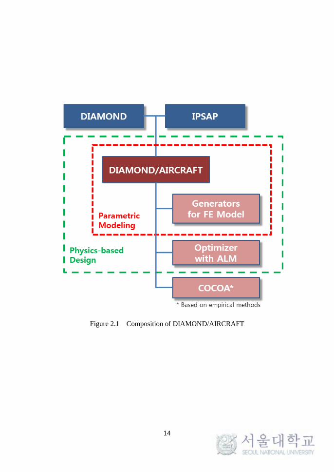
Our design framework is designated as ‘DIAMOND/AIRCRAFT’.
Figure 2.1 shows composition of the design framework, which has three
generators for OML and FE model generation as follows: wing generator,
fuselage generator, and empennage generator. First, the outer mold line (OML)
of aircraft is defined through those generators using parametric modeling
technique. The internal structural layout is also determined at the same time,
which is followed by FE mesh generation. With the design loads applied to FE
mesh, structural members are sized through a physics-based approach, FEM.
At this moment, various design criteria are considered as constraints of
optimization, and multi-level optimization method is adopted to enhance
computational efficiency for faster convergence. The application of a high
fidelity method such as FEM is desirable in order to increase the confidence
for decision-making and reduce the design risk. Figure 2.2 shows the design
procedure for aircraft design using DIAMOND/AIRCARFT.
14
Figure 2.1 Composition of DIAMOND/AIRCRAFT

15
Figure 2.2 Design Procedure in DIAMOND/AIRCRAFT

16
2.2 Literature Survey
The necessity of parametric modeling for aircraft design is evidently
recognized in Chapter 1. Now, the previous studies for parametric modeling
by other researchers are investigated to understand their contents of research.
Mawhinney et al. [7] proposed geometry-based approach for aircraft
conceptual design to efficiently integrate the analysis and design method.
They show that aircraft geometry is generated with the use of displacement,
rotation, and profile components. Using the geometric information, three
kinds of geometric models can be generated for the related analysis: skeleton,
and surface, and solid models. The skeleton model is suitable for loading and
structural analysis, while the surface and solid models are for aerodynamic
analysis. Consequently, the model for structural analysis is unrealistic and
undesirable in terms of the level of fidelity. Rodriguez et al. [5] developed
RAGE (RApid Geometry Engine) in order to create the aircraft geometry for
preliminary design analysis without excessively sophisticated CAD. RAGE is
composed in object-oriented JAVA programming language. RAGE utilizes a
component-based approach to generate geometric models of the aircraft. Main
components include fuselages, wings, and nacelles. They claimed that the
geometric model is mathematically built using the design parameters directly
in RAGE unlike in CAD software that creates splined surfaces. RAGE can
export geometric models formats for aerodynamic analysis tools such as
PLOT3D and PANAIR. La Rocca et al. [30] proposed high-level geometry
primitives in order to help the design engineer generate automated aircraft
geometry. Once picking parameterized geometric elements from database

17
instead of CAD-based elements such as points, lines, and curves, the design
engineer can obtain the geometry of a concept configuration. Although the
proposed method makes the design process efficient and productive through
fast performance, the fidelity is limited and difficult to expand due to the
code-based characteristics.
Researchers working at NASA proposed RAM (Rapid Airplane
Modeler) [4] and VSP (Vehicle Sketch Pad) [6], sequentially released in 1996
and 2010, respectively. RAM was developed written in C++ language to
generate 3-D geometry of aircraft quickly and easily in user-friendly
environment for conceptual design. There are four main components in RAM:
wing, fuselage, external store such as fuel tank and missiles, and engine
including nacelle and duct. Each component is defined by its own parameters.
But, it shows a limited capability to export the geometric model in formats for
vortex lattice method (VLM) and CFD analysis. With the successful
experience of developing RAM, VSP was developed as a modified and
advanced modeler. It enables improving the ability to easily define geometry
by design parameters and displaying in real-time the results of such geometric
definition on GUI. VSP was simply used to provide synthesis code such as
ACSYNT and FLOPS with wetted areas and volumes of an aircraft. VSP can
also generate meta-models to perform high fidelity method, for example,
AWAVE (supersonic compressibility drag analysis program), VorLax (vortex
lattice flow solver), FPS3D (full potential flow solver), and MUSEC (Euler
flow solver). Similar to RAGE and RAM, however, VSP concentrates on the
meta-model generation mostly for aerodynamic analysis as well. For

18
structural analysis, VSP is capable of generating only elements with full depth
such as ribs, spars, and bulkheads for internal structural layout, while it cannot
generate partial depth elements such as stringers and stiffeners for the detailed
modeling of structure.
2.3 Heritage from ASTL
The main objective of DIAMOND/AIRCRAFT is to improve the design
process efficiency and accuracy through a parametric modeling and physics-
based approach using finite element analysis. In order to design structural
components close to real ones as accurately as possible, various design criteria
can be selectively applied to structural sizing. Most of functions of
DIAMOND/AIRCRAFT are implemented under the environment of
DIAMOND/IPSAP, which is the integrated finite element analysis software
with OpenCASCADE-based Graphic User Interface (GUI) for pre/post
processing. DIAMOND/IPSAP was developed and released by ASTL
(Aerospace STructures Laboratory) of the Seoul National University. This
software enables parallel computing process using domain-wise MFS (Multi
Frontal Solver) as well as serial computing process, thus showing excellent
performance speed and improved computational accuracy for finite element
analysis. Hence, DIAMOND/IPSAP has the advantage of computational
capability adequate to solve large-scale problems for complex aerospace
structures such as aircraft, satellite, and launch vehicle.[31,32] It is notable
that DIAMOND/AIRCRAFT has accordingly such an excellent heritage from
DIAMOND/IPSAP.

19
Figure 2.3 Feature of DIAMOND/IPSAP

20
2.4 Design Framework using Parametric Modeling
Each generator defines the configuration of object via handling simple
parameters input and at the same time generate FE mesh for the corresponding
part out of entire aircraft after reflecting internal structural layout. All results
from three generators can be merged collectively when FE mesh of entire
aircraft is required. The preview function of GUI is very helpful during
iterative modification because the change of FE meshes can be immediately
displayed and checked as soon as design parameters change.
2.4.1 Wing Generator
First of all, airfoil selection should be performed as shown Figure 2.4
in order to determine the configuration of main wing. The information on
geometry of three airfoils and each location along the span-wise direction of
wing are required at GUI of wing generator. Airfoil coordinates data can be
imported by text file format or by manual key-in and might be amended
directly on GUI if necessary
Main wing can be divided into two segments such as inboard wing
and outboard wing. Wing OML can be roughly determined by chord lengths at
root and tip of wing, semi-span, sweep back angle, airfoil data, and something
about flaps. DIAMOND/AIRCARFT can produce the structural model
considering the secondary structure as well as the primary structure, while
other similar design tools can deal with the primary structure only. For more
detailed structural layout such as the chord-wise location of front and rear
spars, the number of ribs, the number of stringers, and the attachment between

21
wingbox and secondary structures, tens of figures are needed as shown in
Figure 2.5. In case of two spar structure, the front spar is typically located in
the region near about 15 percent of the chord, and the rear spar at 55-60
percent. [33] The location of spars can be determined when sufficient space
for the housing of control surfaces, high lift devices, their actuating systems,
and de-icing device is obtainable. The locations of ribs are very important
from view of structural stability because they not only postpone local
buckling on the skin but also have relation to attachment of powerplants,
stores, and landing gear structure. All the design parameters on GUI can be
exported for the next trial or another use in the format of text file. The design
parameters for wing configuration and structural layout are summarized in
Table 2.1.
The center wingbox in inboard wing area withstands applied loads
from flight conditions. It is widely known that the stiffened panel concept is
efficient for the load-carrying structure with respect to the weight reduction,
which consists of skins and stringers. In order to create FE mesh of wing,
four-node shell element is utilized for modeling the upper and lower skins, the
spars, the ribs, and the like, and two-node beam element for modeling the
stringers, spar cap, and the like. Figure 2.6 shows FE model generated for
wing via parametric modeling.

22
Figure 2.4 Airfoil Information for Main Wing
Figure 2.5 GUI for Wing Parameters

23
Table 2.1 Design Parameters for Wing
Purpose Design Parameters
Configuration
Chord length at Wing Root & Tip
Wing Semi-Span
Sweepback Angle
Dihedral Angel
Location of the Flap Housing
Span of Inner & Outer Flap
Structural Layout
Number of Stringers at Wing Root & Tip
Number of Ribs
Location of Front & Rear Spars for Wing
Location of Front & Rear Spars for Inner &
Outer flaps

24
Figure 2.6 FE Model of Wing via Parametric Modeling

25
2.4.2 Fuselage Generator
Just as airfoil determination is the first step for wing modeling mentioned
earlier, so cross section definition is for fuselage modeling. Figures 2.7-2.9
show GUIs of fuselage generator, precisely speaking, divided into center
fuselage, aft center fuselage, and aft fuselage. For center fuselage with
constant section, two radii are required for the definition of cross section. The
data on window and door such as quantities and dimensions is required for
fuselage configuration as shown in Figure 2.7. In order to define structural
layout of the fuselage, the number of frames and stringers, and the location of
floor and its supporting structures are needed. By default, all the frames are
equally spaced along the length of center fuselage, but the location of each
frame is promptly editable on GUI. Similarly, the location of stringers is
equally spaced but also editable along the perimeter of fuselage. For aft
fuselage, most of all, the arrangement of frames should be located after
considering the attachment to empennage because there is a load path between
fuselage and empennage. Some frames in aft fuselage are installed with a
tilting angle in order to ensure load path from vertical stabilizer to fuselage.
The design parameters for fuselage are summarized in Table 2.2.
Compared with that of wing structure, the load level of fuselage
generally tends to be lower. But, when structural design is performed, special
attention should be paid because fuselage structure has a number of cut-outs
such as doors, windows, landing gear, and the like, which are structurally
vulnerable at the outer end. Moreover, pressurization might be considered one

26
of load conditions, especially for skin design, because the cabin of transport
aircraft is mostly pressurized. The pressurization of the cabin will be
importantly allowed for from the fatigue aspect after the early design phase.
In DIAMOND/AIRCRAFT, it is easy to apply the load due to pressurization
to FE model of fuselage as shown in Figure 2.10.
Generally, the fuselage skin bears shear load as well as the load due
to pressurization and is supported by stringers and frames to prevent stress
concentration and local buckling. In DIAMOND/AIRCRAFT, fuselage skins
and floor panel are modeled using four-node shell element for FE model.
Fuselage skin is reinforced by frames, stringers and supporting structure,
where they are modeled using two-node beam element. Figure 2.10 shows FE
model of fuselage with an interface for pressurization load.

27
Figure 2.7 GUI for Center Fuselage Parameters
Figure 2.8 GUI for Aft Center Fuselage Parameters

28
Figure 2.9 GUI for Aft Fuselage Parameters
Figure 2.10 FE Model of Fuselage via Parametric Modeling

29
Table 2.2 Design Parameters for Fuselage
Purpose Design Parameters
Configuration
Center
Fuselage length
Radius of Width, Radius of Height
Number, Location, and Dimension of
Windows
Number & Dimension of Doors
Aft Center Fuselage length
Radius of Width, Radius of Height
Aft Fuselage length
Upper Radius, Lower Radius
Structural Layout
Center
Number of Frames
Number of Stringers
Location of Floor Panel
Location of Supporting Structure
Aft Center
Number of Frames
Location of Floor Panel
Location of Supporting Structure
Aft Locations and Tilt Angles of Frames

30
2.4.3 Empennage Generator
Most of design parameters of empennage consisting of vertical and horizontal
stabilizers are basically similar to those of wing. In the same manner, each
OML is defined by three airfoil coordinates, chord lengths at root and tip, and
span for both of vertical and horizontal stabilizer. With respect to structural
layout, empennage might be modeled as multi-cell structure with multiple
spars in order to resist external loads effectively. Figures 2.11-2.12 show the
GUI for parameters of vertical and horizontal tails. The design parameters for
empennage configuration and structural layout are summarized in Table 2.3.
Figure 2.13 shows FE model of empennage via parametric modeling.
Consequently, finite element model of entire aircraft is shown in Figure 2.14
including fuselage, wing, and empennage.
Figure 2.11 GUI for Empennage Parameters: Vertical Tail

31
Figure 2.12 GUI for Empennage Parameters: Horizontal Tail
Figure 2.13 FE Model of Empennage via Parametric Modeling

32
Table 2.3 Design Parameters for Empennage
Purpose Design Parameters
Configuration
HT
Chord length at Root & Tip
Semi-Span
Sweepback Angle
VT Chord length at Root & Tip
Semi-Span
Structural Layout
HT
Number of Stringers
Number of Ribs
Location of Interface Rib with VT
Gap from the Center Line
VT
Number of Stringers
Number of Front Ribs & Rear Ribs
Location and Sweepback Angle of Spars

33
Figure 2.14 FE Model of Entire Aircraft via Parametric Modeling

34
Chapter 3 Design Criteria
3.1 Overview
In Chapter 2, the procedure of generating the FE structural model using
parametric modeling technique is explained for a physics-based design. When
FE analysis is performed with the FE model generated, design criteria must be
required to evaluate whether the structure can withstand the external forces
which are expected to be imposed under the design load conditions.
The conventional approaches for minimum weight design of
complex aircraft structures such as wing, fuselage, and empennage were based
on the fully stressed design (FSD) method.[34] The FSD optimality[35]
means that each member of the structure for the optimal design is fully
stressed by at least one of the design load conditions considered. The FSD
method is applied to structures that are subject to only stress and minimum
gage constraints.
In addition to the FSD, the stability analysis such as buckling and
crippling is performed for beam and shell elements in this study. The critical
buckling stress of beam structure is calculated using Euler buckling equation.
For shell structure including skin, spar, and rib, analytic buckling equation is
also utilized, which is extended from 1-D Euler buckling equation. For
crippling analysis, two semi-empirical methods based on a great deal of
experiments data are available: Needham method and Gerard method.
Furthermore, a local post-buckling analysis is also addressed considering the
effective width for the stringer design.
35
3.2 Buckling Criteria
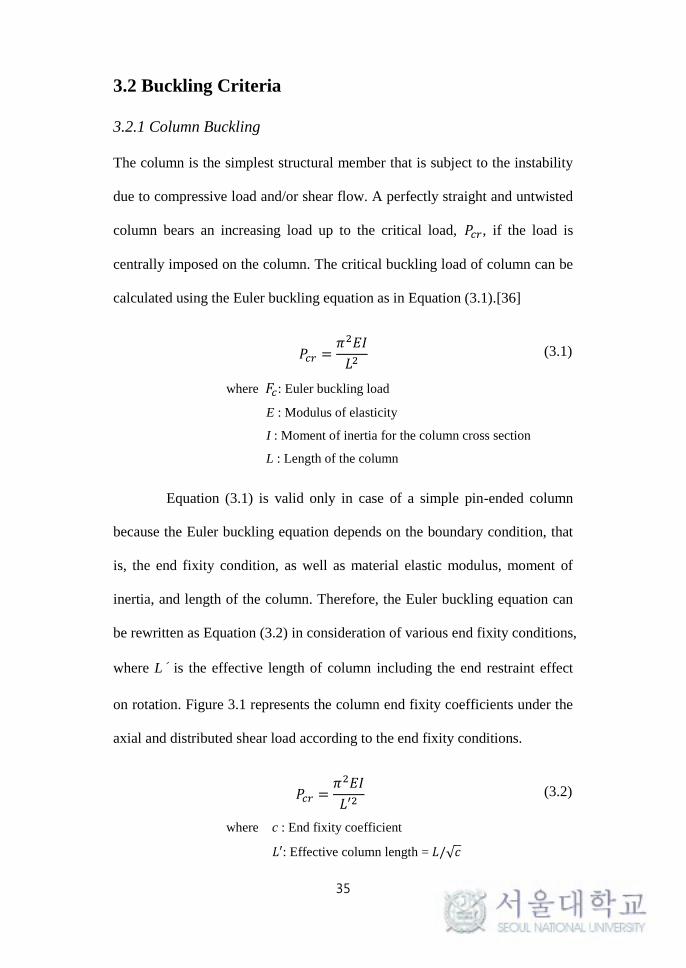
3.2.1 Column Buckling
The column is the simplest structural member that is subject to the instability
due to compressive load and/or shear flow. A perfectly straight and untwisted
column bears an increasing load up to the critical load, 𝑃𝑐𝑟, if the load is
centrally imposed on the column. The critical buckling load of column can be
calculated using the Euler buckling equation as in Equation (3.1).[36]
𝑃𝑐𝑟 =𝜋2𝐸𝐼
𝐿2 (3.1)
where 𝐹𝑐: Euler buckling load
E : Modulus of elasticity
I : Moment of inertia for the column cross section
L : Length of the column
Equation (3.1) is valid only in case of a simple pin-ended column
because the Euler buckling equation depends on the boundary condition, that
is, the end fixity condition, as well as material elastic modulus, moment of
inertia, and length of the column. Therefore, the Euler buckling equation can
be rewritten as Equation (3.2) in consideration of various end fixity conditions,
where L′ is the effective length of column including the end restraint effect
on rotation. Figure 3.1 represents the column end fixity coefficients under the
axial and distributed shear load according to the end fixity conditions.
𝑃𝑐𝑟 =𝜋2𝐸𝐼
𝐿′2 (3.2)
where c : End fixity coefficient
𝐿′: Effective column length = 𝐿/√𝑐

36
With respect to stress instead of force, Equation 3.2 can be also rewritten by
introducing the slenderness ratio term, 𝐿′/𝜌 as Equation (3.3).
𝐹𝑐𝑟 =𝑃𝑐𝑟𝐴=
𝜋2𝐸
(𝐿′/𝜌)2 (3.3)
where c : End fixity coefficient
𝜌: Radius of gyration of column cross section (=√𝐼/𝐴)
A: Area of column cross section
When the critical stress is beyond the proportional limit, elastic modulus (E)
in Equation (3.3) will be replaced with tangent modulus of elasticity (Et).
Among the structural members of aircraft, the stringer of wing,
fuselage, and empennage, and the frame of fuselage are modeled as the
column structure using the beam element in FEM. As a design criterion of
column buckling, the ratio of the actual one to the critical stress, as shown in
Equation (3.4), is checked during the optimization process.
𝐹
𝐹𝑐𝑟− 1 ≤ 0 (3.4)

37
Figure 3.1 Column End Fixity Coefficients [36]

38
3.2.2 Shell Buckling
The buckling equation for thin sheet is derived from the Euler column
buckling equation. In this study, both compression buckling and shear
buckling can be considered for the skin, the spar, and the rib design. The
corresponding buckling equations are shown in Equations (3.5) and (3.6).
[36,37] Figures 3.2 and 3.3 show the buckling coefficient curves for
compression and shear load, respectively. [37]
𝜎𝑐𝑟 =𝜋2𝑘𝑐𝐸
12(1 − 𝜈𝑒2)(𝑡
𝑏)2
(3.5)
where b : Plate length at loaded edge
E : Modulus of elasticity
𝑘𝑐: Compressive buckling coefficient
𝜈𝑒: Posisson’s ratio
𝜏𝑐𝑟 =𝜋2𝑘𝑠𝐸
12(1 − 𝜈𝑒2)(𝑡
𝑏)2
(3.6)
where b : Plate length at loaded edge
E : Modulus of elasticity
𝑘𝑠: Shear buckling coefficient
𝜈𝑒: Posisson’s ratio
Similar to the column buckling, the ratio of the actual one to the
critical stress, as shown in Equation (3.7) and (3.8), is checked during the
optimization process. The interaction equation of combined shear and
compression is shown in Equation (3.9), while the margin of safety in
Equation (3.10).
𝜎
𝜎𝑐𝑟− 1 ≤ 0 (3.7)

39
𝜏
𝜏𝑐𝑟− 1 ≤ 0 (3.8)
𝑅𝐿 + 𝑅𝑆2 = 1.0 (3.9)
𝑀. 𝑆. =2
(𝑅𝐿 +√𝑅𝐿2 + 4𝑅𝑆
2)
− 1 (3.10)
But, it is uncomfortable and frustrating to find a required value from
these coefficient curves in Bruhn[37]. Furthermore, in order to utilize the
curves in computer programming, the coefficient curve must be expressed as a
function, for example, a polynomial function. Hence, the point data were
extracted from the image of coefficient curves using an open source freeware
called ‘Engauge Digitizer 5.1’[38], which can convert an image file showing a
graph into numbers. Then the point data obtained were transformed to a
polynomial function through the simple curve fitting.

40
Figure 3.2 Compressive Buckling Coefficients for Flat Rectangular Plates [37]

41
Figure 3.3 Shear Buckling Coefficients for Flat Rectangular Plates [37]

42
Figure 3.4 Interaction Equation for Combined Shear and Compression [37]

43
3.3 Crippling Criteria
For the prediction of crippling failure, it is necessary to rely on test
results and use empirical methods. Compressive crippling is defined as an
inelasticity of the cross section o f a structural member in its own plane rather
than along its longitudinal axis. [37] It is notable that the maximum crippling
stress of a member is a function of its cross section rather than its length. The
crippling stress for a given section is calculated with the assumption that the
stress is uniform over the entire section although it is actually not uniform. So,
parts of the section might buckle at a stress below the crippling stress, and the
more stable area such as intersection and corners reach a higher stress than the
buckled members as shown in Figure 3.5.
Figure 3.5 Cross Section Subjected to Crippling Stress [36]

44
DIAMOND/AIRCRAFT provides two methods in order to calculate a
crippling stress: Needham method and Gerard method. In Needham method,
the member section is broken down into angle units or segments. From a
study of test data on various types of cross sections, the following crippling
stress equation for angle sections was derived as shown in Equation (3.11).[37]
Figure 3.6 represents the curves for determining the crippling stress of angle
units in accordance with Equation (3.11).
𝐹𝑐𝑠/(𝐹𝑐𝑦𝐸)12 = 𝐶𝑒/(𝑏
′/𝑡)0.75 (3.11)
where 𝐹𝑐𝑠: Crippling stress
𝐹𝑐𝑦: Compression yield stress
E: Modulus of elasticity
𝑏′/𝑡 : Equivalent b/t of section = (a+b)/2t
𝐶𝑒: Coefficient that depends on the degree of edge support
Table 3.1 represents the type of basic angle units and each
coefficient (𝐶𝑒) according to edge conditions. The failing strength of angle
section can be computed by dividing the section into a series of angle
segments and summing the crippling loads for each segment in a weighted
average sense as shown in Equation (3.12).[37]
𝐹𝑐𝑠 = 𝛴(crippling loads of angles)
𝛴(area of angles)= 𝛴𝐴𝑖𝐹𝑐𝑠,𝑖𝛴𝐴𝑖
(3.12)

45
Gerard method has given more generalized semi-empirical method of
determining the crippling stress than Needham method. The Gerard method
reflects the distortion effect of the free unloaded edges upon the failing
strength of the member section. The crippling equations of Gerard method are
shown in Equations (3.13) to (3.15).
For sections with distorted unloaded edges,
𝐹𝑐𝑠/𝐹𝑐𝑦 = 0.56 [(𝑔𝑡2/𝐴)(𝐸/𝐹𝑐𝑦)
1/2]0.85
(3.13)
For sections with straight unloaded edges,
𝐹𝑐𝑠/𝐹𝑐𝑦 = 0.67 [(𝑔𝑡2/𝐴)(𝐸/𝐹𝑐𝑦)
1/2]0.40
(3.14)
For 2 corner sections,
𝐹𝑐𝑠/𝐹𝑐𝑦 = 3.2 [(𝑡2/𝐴)(𝐸/𝐹𝑐𝑦)
1/3]0.75
(3.15)
where 𝐹𝑐𝑠: Crippling stress
𝐹𝑐𝑦: Compression yield stress
𝑡 : Element thickness
E : Modulus of elasticity
A : Section area
g : Number of flanges + number of cuts
In the Equations (3.13) and (3.14), the g value means the number of
flanges that make up the section, plus the number of cuts necessary to divide
the section into a series of flanges. Table 3.2 summarizes the g value for
various cross sections. The maximum crippling stress for a composite section
should be limited to the values in Table 3.3 unless test results are obtained to
substantiate the use of higher crippling stresses.

46
Figure 3.6 Dimensionless Crippling Stress vs. b'/t [37]

47
Table 3.1 Basic Angle Unit for Edge Conditions [37]
Condition Shape 𝐶𝑒
Two edges free
0.316
One edge free
0.342
No edge free
0.366

48
Table 3.2 g values for Various Cross Sections in Gerard Method [36]

49
Table 3.3 Maximum Values for Crippling Stress [37]
Type of Section Max. 𝐹𝑐𝑠
Angles 0.7 𝐹𝑐𝑦
V Groove Plates 𝐹𝑐𝑦
Multi-Corner Sections 0.8 𝐹𝑐𝑦
Stiffened Panels 𝐹𝑐𝑦
Tee, Cruciform and H Sections 0.8 𝐹𝑐𝑦
2 Corner Sections (Z, J, Channels) 0.9 𝐹𝑐𝑦

50
3.4 Johnson-Euler Interaction Equation
For the column strength of structural members with relatively thick wall
thickness, Euler’s equation can be used to calculate the critical stress for both
elastic and inelastic instability with the tangent modulus Et used in the
inelastic stress range. But the test results for the members with an open cross
section, such as channel, hat section, and the like, show that such members
with relatively small thickness would follow the path D-E-F-C instead of the
path A-B-F-C in Figure 3.7. In other words, the actual critical stress in the
path D-E-F is less than that from Euler’s equation. The elastic buckling of
some part of the cross section begins to initiate at the point F, and then the
failure for the member involves both elastic buckling and crippling in the path
E-F, which is called the transition region. Johnson-Euler equation in Equation
(3.16) can be used to calculate the column critical stress in the transition
region.[37]
𝐹𝑐 = 𝐹𝑐𝑠 −𝐹𝑐𝑠2
4𝜋2𝐸(𝐿′/𝜌)2 (3.15)

51
Figure 3.7 Johnson-Euler Interaction Curve [37]

52
3.5 Material Strength
Material strength criteria is applied using Equation (3.16). For the fatigue
dominant structure such as lower skin of wing, it is important that fatigue
analysis must be considered with respect to damage tolerant design. In the
early design phase, however, the load spectrum for fatigue might not
developed. So we instead utilize the ultimate design cut-off stress for damage
tolerant design, which is less than static ultimate strength. For example, the
ultimate design cut-off stress for Al 2024 is 45,000 psi.[36]
𝐹
𝐹𝑐− 1 ≤ 0 (3.16)

53
Chapter 4 Multi-level Optimization
4.1 Overview
The feature of structural design of aircraft with a complex layout leads to a
huge-sized mathematical problem with a great deal of design variables
accordingly. Hence, the multi-level optimization approach is adequate to
solving such a large-scale problem efficiently, where the original problem in
the global level can be divided into a set of small subproblems in the local
level to be more easily solved.[39,40]
First, at the global level, FE analysis of whole structure is performed
in order to calculate internal forces which are required for the evaluation of
structural integrity at local level. In the second step, local design variables
such as dimensions of stringer and thicknesses of skin and rib are optimized in
consideration of design criteria for beam and shell structures. In addition,
local post-buckling instability is also investigated for skin-stringer structures.
At the moment, aforementioned design criteria play a major role as constraints
in optimization process. Then the design variables optimized in the local level
are provided to the global level in order to re-calculate internal forces and
effective width for the next iteration in the local level. Such a sequential
scheme mentioned earlier is repeated as shown in Figure 4.1 until all
convergence conditions are satisfied. As optimization algorithm, augmented
Lagrangian method (ALM) is employed, which is known to be useful for
handling design constraints for efficient computations.

54
4.2 Literature Survey
In order to design and analyze a complex aerospace structure using numerical
modeling, enormous computational resources are required because such a
structure have a great deal of design variables for design engineers to define
its geometry. Generally, the amount of computational resources required is
proportional to the size of numerical problem in question. Furthermore, the
direct solution of a large-scale problem would frequently bring about the
performance problem such as a poor convergence. In this case, one of the
solutions is to break down a large-scale optimization problem into a series of
smaller subproblems. Such uncoupled subproblems can be efficiently
processed using parallel computing technique which is widely used for
aerospace research in recent years. To decompose a large-scale problem into
smaller problems is prevalent in MDO for the development of aerospace
vehicles. During the development, a lot of disciplines would cooperate with
each other, while each discipline preserves its own autonomy from other
disciplines in order to concentrate on the specific area of expertise.
Stimulated by the need to decompose the large task into smaller tasks
that can be performed in parallel, many decomposition schemes and
associated optimization procedures have been proposed until now.
Decomposition approach generally not only reduces total computational cost
but also generates smaller tasks that are adequate to concurrent operations.
Sobieszczanski-Sobieski developed a procedure called the concurrent
subspace optimization (CSSO). [41] It allocates the design variables uniquely
to subspaces that correspond to subsystems. A separate optimization is

55
performed within each subspace with respect to its own design variables. But,
the application without move limits may cause the convergence problem. [42]
Kroo and his colleagues [43–45] proposed another procedure that is known as
collaborative optimization (CO). Since then, many other researchers have
developed variants of CO and applied it to a number of various design
problems. Braun et al. [45] applied this approach to the design of space launch
vehicles, and Sobieski and Kroo [46] applied it to the aircraft configuration
design. These MDO schemes mentioned above can be adapted to multi-level
structural optimization by substituting a module or a discipline with a
substructure.
Researchers including Schmit and Sobieszczanski-Sobieski had
carried out early researches for multi-level formulations. [47–50] Schmit and
Ramanathan [47] presented a multi-level approach for minimum weight
structural design of truss and wing structures in consideration of local and
system buckling constraints. The optimal design of structure is achieved in the
system level subject to strength, displacement, and system buckling
constraints, while the component design is performed in the component level
satisfying local buckling constraints. Their key idea is to select the objective
function in the component level in order to minimize disturbance of loading in
the component level due to component level synthesis. Sobieszczanski-
Sobieski and Loendorf [49] developed a mixed-optimization method
combining mathematical programming to relatively small components and
FSD for large structural assemblies of aircraft fuselage. Sobieszczanski-
Sobieski et al. [50] proposed a more general multi-level approach. They

56
proposed a method for decomposing an original problem into a set of
subproblems and a coordination problem that preserves coupling between
subproblems. They used a cumulative measure of the constraint violation as a
function of element forces and stiffness. Sobieszczanski-Sobieski [51] also
developed a new method for two-level structural optimization called BLISS/S.
In the substructure optimization, local cross sections are optimized as design
variables under the highly nonlinear local constraints of strength and buckling,
while the global design variables govern the overall structure shape under the
displacement constraints.
Based on the multi-level optimization schemes mentioned earlier,
many practical researches for industrial application have been also carried out.
Williams et al. [52] developed the program for exact vibration and buckling
analysis/design called VICONOPT that incorporates the earlier program
VIPASA[53] and VICON[54]. In VICONOPT, Lagrange multipliers are used
to minimize the total energy of the panel subject to constraints. Bushnell [55–
57] developed the program PANDA2, for the design analysis of flat or curved
laminated composite panels. Discretized models of panel cross-sections are
applied to calculate local and global buckling loads. Carrera et al. [58]
developed the two-level optimization tool called NAPAO using NASTRAN
and PANDA2 for the design of CRV (Crew Return Vehicle), where
NASTRAN is used to calculate the loads acting on the panel and the panels
are optimized using PANDA2. The optimal solution is obtained taking into
account buckling and local post-buckling constraints using NAPAO.
Bindolino et al. [18] proposed multi-level structural optimization method with

57
three levels in order to estimate the weight of wingbox of a commercial
aircraft through physics-based approach. In the first level, beam model is used
to optimize the global behavior of the wing. The optimization for cross
section is performed for sizing structural members and selecting a topology of
cross section among four models. In the third level, 3-D FE model is
generated by means of data from previous levels. The constraints for stress,
displacement, and flutter behavior are applied. Dorbath et al. [20] introduced a
design tool for wing mass estimation. They extend the structural model
beyond the primary structure. ELWIS (finite ELment WIng Structure) is used
as the central model generator. Structural analysis and sizing are carried out
using the module called Sizing Robot+. The xml-based DLR data model
CPACS (Common Parametric Aircraft Configuration Scheme) is used as
input and output format.

58
Figure 4.1 Flow Chart for Multi-level Optimization

59
4.3 Global Level vs. Local Level in MLO
The problem statement of general optimization with both equality and
inequality constrains is casted as the following form:
min 𝑥 𝑓(𝑥) (4.1)
Subject to ℎ(𝑥) = 0, 𝑔(𝑥) ≤ 0
where 𝑥 ∈ ℝ𝑛, 𝑓: ℝ𝑛 → ℝ, ℎ: ℝ𝑛 → ℝ𝑚, 𝑔: ℝ𝑛 → ℝ𝑟
The design optimization of aircraft structures generally requires lots
of consideration about complicated and interactive phenomena related to
different disciplines, at least structural mechanics and aerodynamics. Thus it
is not tractable to handle a big problem of the whole structure with a large
number of DOFs at the same time with respect to computational efficiency
and required resources, especially for optimization that requires a number of
iterations. In this case, multi-level optimization approach is quite adequate in
order to reduce time and cost for computation, which can replace the original
problem with multi-level problem in order to solve a set of smaller problems.
For aircraft wing, for example, the global problem is for the whole wing
structure, and the local problem is for a part of wing, the stiffened panel with
skin and stringers. The local-level optimization is performed through bay-by-
bay analysis. Each bay is bounded between two adjacent ribs. The skin in
local system is bounded in front and rear spars along the chord-wise direction
and between two ribs along the span-wise direction, as shown in Figure 4.2.

60
Figure 4.2 Global Level and Local Level in MLO

61
4.4 Augmented Lagrangian Method
4.4.1 Mathematical Formulation
The original problem for constrained optimization can be transformed into an
unconstrained problem with approximation. With respect to mathematical
optimization, relaxation is one of approximation strategy, that is, a
substitution of a difficult original problem with an approximated problem
which can be more easily solved. The constraint functions are added to the
objective function as penalized terms instead of applying the strict constraints
in the optimization. A solution of the relaxed problem provides information
on the original problem. It was already proven that it is optimal for the
original problem if an optimal solution for the relaxed problem is feasible for
the original problem.
Generally, the quadratic penalty method is one of the most popular
approaches, which adds the squares of the constraint violations to the original
objective. This approach is widely used in engineering field due to its
simplicity but has ill-conditioning characteristics inherently.[59] In this study,
Augmented Lagrangian Method (ALM)[59–61] is utilized in order to solve
the optimization problem. The ALM is different from the quadratic penalty
method in that it avoids the possibility of ill-conditioning by introducing
additional Lagrangian multiplier term into the objective function, while it is
similar to the quadratic penalty method in that the constrained problem can be
replaced with a sequence of unconstrained problems. Unlike the penalty, the
augmented Lagrangian function generally keeps smoothness.

62
We begin with the following Equation (4.2) resulted from Equation (4.1) with
both equality and inequality constraints. A vector of additional slack variables
z are introduced to transform inequality constraints into equality ones.
min 𝑥 𝑓(𝑥) (4.2)
Subject to ℎ1(𝑥) = ⋯ = ℎ𝑚(𝑥) = 0,
𝑔1(𝑥) + 𝑧12 = ⋯ = 𝑔𝑟(𝑥) + 𝑧𝑟
2 = 0
where 𝑥 ∈ ℝ𝑛, 𝑓: ℝ𝑛 → ℝ, ℎ: ℝ𝑛 → ℝ𝑚, 𝑔: ℝ𝑛 → ℝ𝑟
First, the augmented Lagrangian for Equation (4.2) is as follows:
�̅�𝐴(𝑥, 𝑧, 𝜆, 𝜇) = 𝑓(𝑥) + 𝜆′ℎ(𝑥) +
1
2𝑐|ℎ(𝑥)|2
+ ∑{𝜇𝑗[𝑔𝑗(𝑥) + 𝑧𝑗2] +
1
2𝑐
𝑟
𝑗=1
|𝑔𝑗(𝑥) + 𝑧𝑗2|2}
(4.3)
Here, we should minimize the augmented Lagrangian, in Equation
(4.3) with respect to (x, z) for various multipliers, 𝜆 and 𝜇, and penalty
parameter c. Equation (4.4) can be written because the minimization of
Equation (4.3) can be performed explicitly for each fixed x. Then, the
minimization of Equation (4.4) with respect to z is equivalent to Equation (4.5)
which is expressed in the quadratic form of 𝑢𝑗 representing the square of 𝑧𝑗.
min𝑧�̅�𝐴(𝑥, 𝑧, 𝜇) = 𝑓(𝑥) + 𝜆
′ℎ(𝑥) + 1
2𝑐|ℎ(𝑥)|2
+ ∑min𝑧𝑗{𝜇𝑗[𝑔𝑗(𝑥) + 𝑧𝑗
2] + 1
2𝑐
𝑟
𝑗=1
|𝑔𝑗(𝑥) + 𝑧𝑗2|2}
(4.4)
min 𝑢𝑗≥0
{𝜇𝑗[𝑔𝑗(𝑥) + 𝑢𝑗] + 1
2𝑐 |𝑔𝑗(𝑥) + 𝑢𝑗|
2} (4.5)

63
Differentiating Equation (4.5) with respect to 𝑢𝑗 and then substituting 𝑢𝑗
with �̂�𝑗 at which the derivative is zero, we finally obtain Equation (4.6).
�̂�𝑗 = −[(𝜇𝑗/𝑐) + 𝑔𝑗(𝑥)] (4.6)
Because �̂�𝑗 must be either �̂�𝑗 ≥ 0 by which Equation (4.5) is solved or
equal to zero, the solution of Equation (4.5) can be written as Equation (4.7).
𝑢𝑗∗ = max{0,−[(𝜇𝑗/𝑐) + 𝑔𝑗(𝑥)]} (4.7)
In order to express Equation (4.3) in a simple form, we define the notation
𝑔𝑗+ as follows:
𝑔𝑗(𝑥) + 𝑢𝑗∗ = max{𝑔𝑗(𝑥), −(𝜇𝑗/𝑐)} ≡ 𝑔𝑗
+(𝑥, 𝜇𝑗, 𝑐) (4.8)
𝑔+(𝑥, 𝜇, 𝑐) = [
𝑔𝑗+(𝑥, 𝜇1, 𝑐)
⋮𝑔𝑗+(𝑥, 𝜇𝑟, 𝑐)
] (4.9)
With Equations (4.4)-(4.9), Equation (4.3) can be arranged as the following
equation (4.10).
min𝑧�̅�𝐴(𝑥, 𝑧, 𝜆, 𝜇) = 𝑓(𝑥) + 𝜆
′ℎ(𝑥) +1
2 𝑐|ℎ(𝑥)|2
+𝜇′𝑔+(𝑥, 𝜇, 𝑐) +1
2 𝑐|𝑔+(𝑥, 𝜇, 𝑐)|2
(4.10)
Finally, the augmented Lagrangian can be expressed as Equation (4.11)
because it is not the function of the slack variable z any longer.
𝐿𝐴(𝑥, 𝜆, 𝜇) = 𝑓(𝑥) + 𝜆′ℎ(𝑥) + +𝜇′𝑔+(𝑥, 𝜇, 𝑐)
+1
2𝑐{|ℎ(𝑥)|2 + |𝑔+(𝑥, 𝜇, 𝑐)|2}
(4.11)

64
During iterations, Equation (4.11) is solved approximately and then the
Lagrange multipliers and the penalty parameter are updated according to
Equations (4.12) to (4.14), where the superscript k represents k-th iteration. In
this study, we use 𝛼=1.1 as the coefficient for updating the penalty parameter.
𝜆𝑗𝑘+1 = 𝜆𝑗
𝑘 + 𝑐𝑘ℎ(𝑥𝑘) (4.12)
𝜇𝑗𝑘+1 = 𝜇𝑗
𝑘 + 𝑔𝑗+(𝑥𝑘, 𝜇𝑗
𝑘 , 𝑐𝑘) = 𝜇𝑗𝑘 +max{𝑔𝑗(𝑥), −(𝜇𝑗/𝑐)} (4.13)
𝑐𝑘+1 = 𝛼𝑐𝑘, 𝛼 > 1 (4.14)
Figures 4.3 and 4.4 show the flow charts of augmented Lagrangian
method and Newton method, respectively. In ALM code, Newton method is
utilized to find a search direction during the optimization, where the gradient
and hessian of constraint functions are calculated.

65
Figure 4.3 Flowchart of Augmented Lagrangian Method (ALM)

66
Figure 4.4 Flowchart of Newton Method in ALM

67
4.4.2 Test Problem for Code Validation
In order to validate the code for ALM formulated in the previous part, the
following optimization problem is introduced and solved with the code.
min 𝑥,𝑦≥0
𝑓(𝑥, 𝑦) = −𝑥1 − 𝑥2 − 2𝑦1 − 𝑦2 (4.15)
Subject to 𝑔1(𝑥, 𝑦) = 𝑥1 + 2𝑥2 + 2𝑦1 + 𝑦2 − 40 ≤ 0
𝑔2(𝑥, 𝑦) = 𝑥1 + 3𝑥2 − 30 ≤ 0
𝑔3(𝑥, 𝑦) = 2𝑥1 + 𝑥2 − 20 ≤ 0
𝑔4(𝑥, 𝑦) = 𝑦1 − 10 ≤ 0
𝑔5(𝑥, 𝑦) = 𝑦2 − 10 ≤ 0
𝑔6(𝑥, 𝑦) = 𝑦1 + 𝑦2 − 15 ≤ 0
Equation (4.15) is one of the optimization problem with a coupled
constraint as seen in the constraint function 𝑔1 of both x and y. For all
variables, four positively bounded constraints are added to the above six
constraint functions, and there are totally ten constrains.
𝑔7(𝑥, 𝑦) = −𝑥1
𝑔8(𝑥, 𝑦) = −𝑥2
𝑔9(𝑥, 𝑦) = − 𝑦1
𝑔10(𝑥, 𝑦) = − 𝑦2
≤ 0
≤ 0
≤ 0
≤ 0
As mentioned earlier, the original constrained problem can be
replaced with the unconstrained dual problem which takes the constraints into
account by augmenting the objective function with a weighted sum of the
constraint functions. Equation (4.15) is transformed into the augmented
Lagrangian function in Equation (4.16)

68
min 𝑥,𝑦,𝜇≥0
𝐿𝐴(𝑥, 𝑦, 𝜇) = 𝑓(𝑥, 𝑦) + 𝜇′𝑔+(𝑥, 𝑦, 𝜇, 𝑐) +
1
2𝑐|𝑔+(𝑥, 𝑦, 𝜇, 𝑐)|2 (4.16)
The initial values for variables are all zero, that is, 𝑥1 = 𝑥2 = 𝑦1 =
𝑦2 = 0. Figures 4.5 and 4.6 show the convergence history of the design
variables and the objective function, respectively. Table 4.1 represents the
convergence history of the objective function and the constraint functions.
As seen in Figure 4.5, the design variables are converged after 8th
iteration. The optimal design point is (𝑥1, 𝑥2) = (8.333, 3.333) and (𝑦1, 𝑦2) =
(10, 5), and then the optimal value of the objective function is -36.667.
According to Figure 4.6, it seems as though the optimal value of the objective
function is already found at 2nd iteration. But it is not the optimal because
some violations for constraint functions are involved when the constraint
functions are checked out. In Table 4.1, the shaded cell represents the
violation for any of constraint functions. Eventually, the optimal design point
can be obtained at 8th iteration, satisfying all the constraint conditions at the
same time.

69
Figure 4.5 Convergence History of Design Variables
Figure 4.6 Convergence History of Objective Function

70
Table 4.1 History of Constraint Functions
Number of
Iterations 1 2 3 4 5 6 7 8
f 0.000 -41.818 -37.017 -36.667 -36.667 -36.667 -36.667 -36.667
𝑔1 -40.000 4.546 -1.405 0.028 -0.002 1.400E-4 1.000E-4 0.000
𝑔2 -30.000 -23.182 -15.744 -11.814 -11.653 -11.668 -11.667 -11.667
𝑔3 -20.000 2.727 0.248 0.028 -0.002 2.200E-4 0.000 0.000
𝑔4 -10.000 5.455 0.496 0.055 -0.005 4.000E-4 0.000 0.000
𝑔5 -10.000 -5.000 -5.000 -5.000 -5.000 -5.000 -5.000 -5.000
𝑔6 -15.000 5.455 0.496 0.055 -0.005 4.000E-4 0.000 0.000
𝑔7 0.000 -12.273 -9.298 -8.379 -8.329 -8.334 -8.333 -8.333
𝑔8 0.000 1.818 -1.653 -3.269 -3.339 -3.333 -3.333 -3.333
𝑔9 0.000 -15.455 -10.496 -10.055 -9.995 -10.000 -10.000 -10.000
𝑔10 0.000 -5.000 -5.000 -5.000 -5.000 -5.000 -5.000 -5.000
※ The numbers in shaded cells mean the violation of constraint condition because they must be less than or equal to zero.

71
4.5 Calculation of Gradient and Hessian Matrix
4.5.1 Gradient of Constraint Functions for Beam
The gradient and Hessian matrix of original objective function and constraint
functions are calculated in Newton method during the optimization. As
mentioned in Chapter 3, the design criteria such as buckling, crippling,
material strength, and bounded variables are involved as the constraint
functions in the optimization process. Although various types of cross
sections can be used in the beam library of DIAMOND/AIRCRAFT, the
formulation for the beam with zee-shaped cross section is presented here.
The objective function for beam in a local system is expressed in
Equation (4.17), where 𝜌𝑚 and V represents the material density and the
volume of the beam, respectively. Then, the gradient and Hessian matrix can
be calculated as Equations (4.18) and (4.19), where only the cross section area
is the function of design variables.
𝑓1(𝑥𝑖) = 𝜌𝑚𝑉 = 𝜌𝑚𝐴(𝑥𝑖)𝐿 (4.17)
𝐺𝑓1 =𝜕𝑓1𝜕𝑥𝑖
= 𝜌𝑚𝐿𝜕𝐴
𝜕𝑥𝑖 (4.18)
𝐻𝑓1 = 𝜌𝑚𝐿𝜕2𝐴
𝜕𝑥𝑖𝜕𝑥𝑗= 𝜌𝑚𝐿
[ 𝜕2𝐴
𝜕𝑥1𝜕𝑥1⋯
𝜕2𝐴
𝜕𝑥1𝜕𝑥𝑛⋮ ⋱ ⋮
𝜕2𝐴
𝜕𝑥𝑛𝜕𝑑1⋯
𝜕2𝐴
𝜕𝑥𝑛𝜕𝑥𝑛]
(4.19)

72
The gradient of constraint functions can be calculated as the
following equations.
Gradient of Crippling Constraint Function
𝐺11(𝑖) =𝜕𝑔11𝜕𝑥𝑖
= −𝜕𝜎𝑛𝜕𝑥𝑖
−𝜕𝐹𝑐𝜕𝑥𝑖
(if 𝜎𝑛 < 0) (4.20)
where 𝜕𝐹𝑐𝜕𝑥𝑖
= (1 −𝐹𝑐𝑠2𝜋2𝐸
(𝐿′/𝜌)2)𝜕𝐹𝑐𝑠𝜕𝑥𝑖
+(𝐹𝑐𝑠𝐿
′)2
2𝜋2𝐸𝜌3𝜕𝜌
𝜕𝑥𝑖
*Derivative of Crippling Stress 𝐹𝑐𝑠 for z-cross section Beam
𝜕𝐹𝑐𝑠𝜕𝑥1
= −2.4 𝐹𝑐𝑦(𝑥32/𝐴)0.75(𝐸/𝐹𝑐𝑦)
0.75/2 1
𝐴
𝜕𝐴
𝜕𝑥1
𝜕𝐹𝑐𝑠𝜕𝑥2
= −2.4 𝐹𝑐𝑦(𝑥32/𝐴)0.75(𝐸/𝐹𝑐𝑦)
0.75/2 1
𝐴
𝜕𝐴
𝜕𝑥2
𝜕𝐹𝑐𝑠𝜕𝑥3
= 2.4 𝐹𝑐𝑦(𝑥32/𝐴)−0.25(𝐸/𝐹𝑐𝑦)
0.75/2(2𝑥3𝐴−𝑥32
𝐴2𝜕𝐴
𝜕𝑥3)
𝜕𝐹𝑐𝑠𝜕𝑡
= −2.4 𝐹𝑐𝑦(𝑔𝑥32/𝐴)0.75(𝐸/𝐹𝑐𝑦)
0.75/2 1
𝐴
𝜕𝐴
𝜕𝑡
(4.21)
Gradient of Buckling Constraint Function
𝐺12(𝑖) =𝜕𝑔12𝜕𝑥𝑖
= −𝜕𝜎𝑛𝜕𝑥𝑖
−𝜕𝐹𝑐𝑟𝜕𝑥𝑖
(if 𝜎𝑛 < 0) (4.22)
where 𝜕𝐹𝑐𝑟𝜕𝑥𝑖
=2𝜋2𝐸𝜌
(𝐿′)2𝜕𝜌
𝜕𝑥𝑖
Gradient of Material Strength Constraint Function
𝐺13(𝑖) =𝜕𝑔13𝜕𝑥𝑖
=
{
𝜕𝜎𝑛𝜕𝑥𝑖
≤ 0 (if 𝜎𝑛 > 0)
−𝜕𝜎𝑛𝜕𝑥𝑖
≤ 0 (if 𝜎𝑛 < 0)
(4.23)

73
The relation of internal force 𝐹𝑖𝑛 and normal stress 𝜎𝑛 is described as
Equation (4.24), and then the partial derivative of internal force with respect
to a design variable 𝑥𝑖 can be expressed as Equation (4.25). Here, we assume
that 𝜕𝐹𝑖𝑛
𝜕𝑥𝑖= 0 because there is no internal force update during the
optimization in the local level.
𝐹𝑖𝑛 = 𝜎𝑛(𝑥𝑖) 𝐴(𝑥𝑖) (4.24)
𝜕𝐹𝑖𝑛𝜕𝑥𝑖
=𝜕𝜎𝑛𝜕𝑥𝑖
𝐴 + 𝜎𝑛𝜕𝐴
𝜕𝑥𝑖≈ 0 (4.25)
Then the partial derivative of normal stress and radius of gyration
with respect to design variable can be expressed as Equations (4.26) and
(4.27). The derivatives of normal stress with respect to design variables are
summarized in Appendix A for the major cross sections of beam.
𝜕𝜎𝑛𝜕𝑥𝑖
= −𝜎𝑛𝐴
𝜕𝐴
𝜕𝑥𝑖 (4.26)
𝜕𝜌
𝜕𝑥𝑖=𝜌
2(1
𝐼
𝜕𝐼
𝜕𝑥𝑖−1
𝐴
𝜕𝐴
𝜕𝑥𝑖) (4.27)

74
4.5.2 Hessian of Constraint Functions for Beam
The Hessian Matrix of constraint functions can be calculated as the following
equations.
Hessian of Crippling Constraint Function
𝐻11(𝑖, 𝑗) =𝜕2𝑔11𝜕𝑥𝑖𝜕𝑥𝑗
= −𝜕2𝜎𝑛𝜕𝑥𝑖𝜕𝑥𝑗
−𝜕2𝐹𝑐𝜕𝑥𝑖𝜕𝑥𝑗
(if 𝜎𝑛 < 0) (4.28)
Hessian of Buckling Constraint Function
𝐻12(𝑖, 𝑗) =𝜕2𝑔12𝜕𝑥𝑖𝜕𝑥𝑗
= −𝜕2𝜎𝑛𝜕𝑥𝑖𝜕𝑥𝑗
−𝜕2𝐹𝑐𝑟𝜕𝑥𝑖𝜕𝑥𝑗
(if 𝜎𝑛 < 0) (4.29)
Hessian of Material Strength Constraint Function
𝐻13(𝑖, 𝑗) =𝜕2𝑔13𝜕𝑥𝑖𝜕𝑥𝑗
=
{
𝜕2𝜎𝑛𝜕𝑥𝑖𝜕𝑥𝑗
(if 𝜎𝑛 > 0)
−𝜕2𝜎𝑛𝜕𝑥𝑖𝜕𝑥𝑗
(if 𝜎𝑛 < 0)
(4.30)
Then the second-order partial derivative of normal stress and radius
of gyration with respect to design variable can be expressed as Equations
(4.31) and (4.32).
𝜕2𝜎𝑛𝜕𝑥𝑖𝜕𝑥𝑗
=2𝜎𝑛𝐴2
(𝜕𝐴
𝜕𝑥𝑖) (𝜕𝐴
𝜕𝑥𝑗) −
𝜎𝑛𝐴
𝜕2𝐴
𝜕𝑥𝑖𝜕𝑥𝑗
(4.31)
𝜕2𝜌
𝜕𝑥𝑖𝜕𝑥𝑗=1
2
𝜕𝐴
𝜕𝑥𝑗(1
𝐼
𝜕𝐼
𝜕𝑥𝑖−1
𝐴
𝜕𝐴
𝜕𝑥𝑖)
+𝜌
2{−
1
𝐼2(𝜕𝐼
𝜕𝑥𝑖)(
𝜕𝐼
𝜕𝑥𝑗) +
1
𝐼
𝜕2𝐼
𝜕𝑥𝑖𝜕𝑥𝑗+1
𝐴2(𝜕𝐴
𝜕𝑥𝑖) (𝜕𝐴
𝜕𝑥𝑗) −
1
𝐴
𝜕2𝐴
𝜕𝑥𝑖𝜕𝑥𝑗 }
(4.32)

75
4.5.3 Gradient of Constraint Functions for Shell
The objective function for shell in a local system is expressed in Equation
(4.33), where 𝜌𝑚 and V represent the material density and the volume of the
beam, respectively. The area of shell element is the function of ‘a’ and ‘b’,
where ‘a’ and ‘b’ represent the width along the x-direction and the height
along the y-direction. But, both of the width and the height of shell are fixed
because they are not considered design variables. Thickness of shell is the
only design variable. Then, the gradient and Hessian matrix can be calculated
as Equations (4.34) and (4.35), where only the cross section area is the
function of design variables. Similar to Equation (4.26) for the beam,
Equation (4.36) is derived for the shell.
𝑓2(𝑡) = 𝜌𝑚𝑉(𝑎, 𝑏, 𝑡) = 𝜌𝑚𝐴(𝑎, 𝑏)𝑡 (4.33)
𝐺𝑓2 =𝜕𝑓2𝜕𝑡
= 𝜌𝑚𝐴 (4.34)
𝐻𝑓2 = 0 (4.35)
𝜕𝜎𝑚𝑛𝜕𝑡
= −𝜎𝑚𝑛(𝑡)
𝑡 (4.36)
For shell buckling, three kinds of constraint functions are considered
as mentioned in Equations (3.7) to (3.10) of Chapter 3.2.2: compression
buckling, shear buckling, and compression-shear combined buckling. For
shell, axial compression buckling is estimated using the stress by the
following rule.
𝜎𝑐 = {𝜎𝑥𝑥 (𝑖𝑓 𝑏 > 𝑎)𝜎𝑦𝑦 (𝑖𝑓 𝑏 < 𝑎)
(4.37)

76
The constraint functions for compression, shear, and compression-shear
combined buckling are expressed as the following equations. Equation (4.40)
for the combined buckling is derived from Equation (3.9).
𝑔21(𝑐)(𝑡) = −𝜎𝑐 − 𝜎𝑐𝑟 ≤ 0, where 𝜎𝑐𝑟 =
𝜋2𝑘𝑐𝐸
12(1 − 𝜈𝑒2)(𝑡
𝑏)2
(4.38)
𝑔21(𝑠)(𝑡) = −𝜏 − 𝜏𝑐𝑟 ≤ 0, where 𝜏𝑐𝑟 =
𝜋2𝑘𝑠𝐸
12(1 − 𝜈𝑒2)(𝑡
𝑏)2
(4.39)
𝑔21(𝑐𝑜𝑚)(𝑡) = 𝜎𝑐𝑟𝜏
2 − 𝜎𝑐𝜏𝑐𝑟2 − 𝜎𝑐𝑟𝜏𝑐𝑟
2 ≤ 0 (4.40)
The gradient of constraint functions can be calculated using the
following equations. But, the shell buckling equation is not used as the
constraint condition during the optimization because shell buckling is allowed
if the effective width method is considered.
Gradient of Combined Buckling Constraint Function
𝐺21(𝑐𝑜𝑚𝑏) =
𝜕𝑔21(𝑐)
𝜕𝑡
=𝜕𝜎𝑐𝑟𝜕𝑡
𝜏2 + 2𝜎𝑐𝑟𝜏𝜕𝜏
𝜕𝑡−𝜕𝜎𝑐𝜕𝑡
𝜏𝑐𝑟2 − 2𝜎𝑐𝜏𝑐𝑟
𝜕𝜏𝑐𝑟𝜕𝑡
−𝜕𝜎𝑐𝑟𝜕𝑡
𝜏𝑐𝑟2 − 2𝜎𝑐𝑟𝜏𝑐𝑟
𝜕𝜏𝑐𝑟𝜕𝑡
(4.41)
Substituting 𝜏𝑐𝑟 = (𝑘𝑠
𝑘𝑐)𝜎𝑐𝑟 and
𝜕𝜏𝑐𝑟
𝜕𝑡= (
𝑘𝑠
𝑘𝑐)𝜕𝜎𝑐𝑟
𝜕𝑡 into (5.29),
𝐺21(𝑐𝑜𝑚𝑏)
=𝜕𝜎𝑐𝑟𝜕𝑡
𝜏2 + 2𝜎𝑐𝑟𝜏𝜕𝜏
𝜕𝑡
− (𝑘𝑠𝑘𝑐)2
{𝜕𝜎𝑐𝜕𝑡
𝜎𝑐𝑟2 + 2𝜎𝑐𝜎𝑐𝑟
𝜕𝜎𝑐𝑟𝜕𝑡
+ 3𝜎𝑐𝑟2𝜕𝜎𝑐𝑟𝜕𝑡
}
(4.42)

77
By Equation (4.36), the derivative function of stress with respect to the skin
thickness is arranged as Equation (4.43). The derivative function of
compression buckling stress is also calculated from Equations (3.5).
𝜕𝜎𝑐𝜕𝑡
= −𝜎𝑐𝑡
(4.43)
𝜕𝜎𝑐𝑟𝜕𝑡
=𝜋2𝑘𝑐𝐸𝑡
6𝑏2(1 − 𝜈𝑒2)
(4.44)
Substituting Equations (5.36) and (5.37) into (5.35),
𝐺21(𝑐𝑜𝑚𝑏)
= −(𝑘𝑠𝑘𝑐)2
(3𝑘𝑐2𝐶𝑏
2𝑡3𝜎𝑐 + 6𝑘𝑐3𝐶𝑏
3𝑡5) (4.45)
where 𝐶𝑏 =𝜋2𝐸
12𝑏2(1 − 𝜈𝑒2)
Gradient of Compression Buckling Constraint Function
𝐺21(𝑐)=𝜕𝑔21
(𝑐)
𝜕𝑡= −
𝜕𝜎𝑐𝜕𝑡
−𝜕𝜎𝑐𝑟𝜕𝑡
= −𝜎𝑐𝑡−
𝜋2𝑘𝑐𝐸𝑡
6𝑏2(1 − 𝜈𝑒2)
(4.46)
Gradient of Shear Buckling Constraint Function
𝐺21(𝑠)=𝜕𝑔21
(𝑠)
𝜕𝑡= −
𝜕𝜏
𝜕𝑡−𝜕𝜏𝑐𝑟𝜕𝑡
= −𝜏
𝑡−
𝜋2𝑘𝑠𝐸𝑡
6𝑏2(1 − 𝜈𝑒2)
(4.47)
Gradient of Material Strength Constraint Function
𝐺22(𝑚𝑛)
=𝜕𝑔22
(𝑚𝑛)
𝜕𝑡= −
𝜕𝜎𝑚𝑛𝜕𝑡
= −𝜎𝑚𝑛(𝑡)
𝑡 (4.48)

78
4.5.4 Hessian of Constraint Functions for Shell
The Hessian Matrix of constraint function can be calculated as the following
equation.
Hessian of Combined Buckling Constraint Function
𝐻21(𝑐𝑜𝑚𝑏)
=𝜕𝐺21
(𝑐𝑜𝑚𝑏)
𝜕𝑡
= −(𝐾𝑠𝐾𝑐)2
{9𝐾𝑐2𝐶𝑏
2𝑡2𝜎𝑐 + 3𝐾𝑐2𝐶𝑏
2𝑡3𝜕𝜎𝑐𝜕𝑡
+ 30𝐾𝑐3𝐶𝑏
3𝑡4}
= −(6𝐾𝑆2𝐶𝑏
2𝑡2𝜎𝑐 + 30𝐾𝑆2𝐾𝑐𝐶𝑏
3𝑡4) (4.49)
Hessian of Compression Buckling Constraint Function
𝐻21(𝑐)=𝜕𝐺21
(𝑐)
𝜕𝑡= −
𝜕𝜎𝑐𝜕𝑡
−𝜕𝜎𝑐𝑟𝜕𝑡
=2𝜎𝑐𝑡2
−𝜋2𝑘𝑐𝐸
6𝑏2(1 − 𝜈𝑒2)
(4.50)
Hessian of Shear Buckling Constraint Function
𝐻21(𝑠)=𝜕𝐺21
(𝑠)
𝜕𝑡= −
𝜕𝜏
𝜕𝑡−𝜕𝜏𝑐𝑟𝜕𝑡
=2𝜏
𝑡2−
𝜋2𝑘𝑠𝐸
6𝑏2(1 − 𝜈𝑒2)
(4.51)
Hessian of Material Strength Constraint Function
𝐻22(𝑚𝑛)
=𝜕𝐺22
(𝑚𝑛)
𝜕𝑡= −
(𝜕𝜎𝑚𝑛𝜕𝑡
) 𝑡 − 𝜎𝑚𝑛
𝑡2=2𝜎𝑚𝑛𝑡2
(4.52)

79
Chapter 5 Preliminary Structural Sizing
5.1 Overview
Recently, the 90-seat turboprop market is emerging as a new sector according
to the airliners’ demand for larger and more cost-efficient turboprop with
respect to the growth of traffic volume and the economic requirements, for
example, operating cost reduction from fuel efficiency. Currently, the
mainstream of turboprop market is 70-seat aircraft such as ATR 72 and Q400.
But, it is expected that the 90-seat turboprop will have competitiveness
because of push-down from 100-seat aircraft as well as push-up from 50-seat
regional jet or 70-seat turboprop deployed when the aspect of fuel economics
is underlined. It is worthy of considering such a market trend to determine the
type of new aircraft that will be developed. Therefore, the design object in this
study is assumed to be a turboprop aircraft which can accommodate 90
passengers on regional flights.
In the following part of this chapter, the preliminary structural design
for wing of a transport aircraft will be carried out. The finite element model is
generated based on parametric modeling technique, and the structural sizing
and the weight estimation are performed using physic-based method, FEM.
The general information of turboprop aircraft used in this study was provided
by Korea Aerospace Research Institute (KARI), with which this dissertation
focuses on the development of design framework and multi-level optimization
routine using ALM.

80
5.2 General Information
5.2.1 Aircraft Configuration
Figures 5.1 shows the configuration of 90-seat turboprop aircraft. According
to TRLs, MTOW of the aircraft is about 70,000 pound. The aircraft has two
5,500-SHP turboprop engines for thrust. The landing gears are installed in the
nacelle on the wing. As seen in Figure 5.1, the wing is high wing type
mounted on the fuselage as the competitor aircrafts. The wing area is 740 ft2,
and wing span is 94.2 ft. The leading edge of wing has uniform sweepback
angle. Figure 5.2 and Table 5.1 show the geometry information of wing.
Based on the OML of wing, the internal structural layout is determined later.
5.2.2 Material Selection
In aerospace industry, aluminum alloys are characterized by an excellent
strength-to-weight ratio, corrosion resistance, workability or formability, and
other predominant characteristics. Among various aluminum alloys, 2000 and
7000 series are the most widely used. The upper skin of wing is made of Al
7150, but the lower skin is made of Al 2024. Al 2024 is generally used for
fatigue-critical tension application. The materials of stringers in upper and
lower skin are Al 7150 and Al 7075, respectively. Al 7150 is used for high
strength major structural applications where weight savings over Al 7075 are
required. In addition, the spar and the rib are made of Al 7050. Table 5.2
summarizes the material selection for the structural parts of wing.
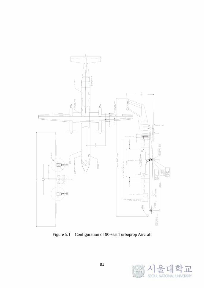
81
Figure 5.1 Configuration of 90-seat Turboprop Aircraft

82
Figure 5.2 Plan View of Wing Layout (Half Span)

83
Table 5.1 Geometry Information of Wing
Geometry Parameter Measurement
Wing Span 94.2 ft
Wing Area 740 ft2
Aspect Ratio 12
Sweepback Angle 5.59 (LE)
Dihedral Angle 2.5
Taper Ratio 0.35
Mean Aerodynamic Chord (MAC) 101.52
Table 5.2 Material Selection for Wing Component
Structural Component Material Selection
Upper Skin Al 7150
Lower Skin Al 2024
Upper Stringer Al 7150
Lower Stringer Al 7075
Spar Al 7050
Rib Al 7050

84
5.3 Problem Statement
In order to find the optimal weight of wing, the global optimization problem is
casted as Equation (5.1), where 𝑓1(𝑥𝑖𝑗, 𝑢) and 𝑓2(𝑡
𝑘, 𝑢) represent the
weight of beam and shell in a local system, respectively.
min𝑥,𝑡
𝑓(𝑥, 𝑡, 𝑢) = min𝑥,𝑡
{∑𝑓1(𝑥𝑖𝑗, 𝑢)
𝑛𝑏
𝑗=1
+∑𝑓2(𝑡𝑘 , 𝑢)
𝑛𝑠
𝑘=1
} (5.1)
where j = the index of beam element
k : the index of shell element
𝑥𝑖𝑗 : i-th design variable in j-th beam element
𝑡𝑘 : thickness in k-th shell element
u : global displacement vector
As mentioned in Chapter 4.3, the local level optimization is
performed through bay-by-bay analysis. The skin in local system is bounded
in front and rear spars along the chord-wise direction and between two ribs
along the span-wise direction. Each panel load’s derivative with respect to
design variable can be assumed to be zero by the assumption that panel loads
change slowly during the optimization. As explained in Figure 4.1, stress and
displacement are updated in the global level, while they are fixed value in the
local level during the optimization. Equation (5.1) can be divided into the
objective functions for a set of local systems, which can be solved
independently. Then, the local level optimization problem can be arranged as
the following Equations (5.2) and (5.3), where 𝜎𝑛 represents the normal
stress of beam.

85
min𝑓1(𝑥𝑖) for beam (5.2)
Subject to 𝑔11(𝑥𝑖, 𝑢(𝑥𝑖)) = −𝜎𝑛 − 𝐹𝑐 ≤ 0 (crippling)
𝑔12(𝑥𝑖, 𝑢(𝑥𝑖)) = −𝜎𝑛 − 𝐹𝑐𝑟 ≤ 0 (buckling)
𝑔13(𝑥𝑖, 𝑢(𝑥𝑖)) ≤ 0 (material strength)
𝑔14(𝑥𝑖) = 𝑥𝑖 − 𝑥𝑖,𝑚𝑎𝑥 ≤ 0 (upper bound)
𝑔15(𝑥𝑖) = 𝑥𝑖,𝑚𝑖𝑛 − 𝑥𝑖 ≤ 0 (lower bound)
min𝑓2(𝑡) for shell (5.3)
Subject to 𝑔21(𝑡, 𝑢(𝑡)) ≤ 0 (comp/shear/combined buckling)
𝑔22(𝑡, 𝑢(𝑡)) ≤ 0 (material strength)
𝑔23(𝑡) = 𝑡 − 𝑡𝑚𝑎𝑥 ≤ 0 (upper bound)
𝑔24(𝑡) = 𝑡𝑚𝑖𝑛 − 𝑡 ≤ 0 (lower bound)
Equations (5.2) and (5.3) can be applied to the case in which the
effective width is not considered. If the effective width is considered for the
panel design, the constraint conditions must be modified. First, among the
constraint functions of Equation (5.2), 𝑔11 and 𝑔12 become the function of t
as well as 𝑥𝑖 and u due to the effective width as shown in Equation (5.4).
𝑔11(𝑥𝑖, 𝑢(𝑥𝑖), 𝑡) ≤ 0 (crippling)
𝑔12(𝑥𝑖, 𝑢(𝑥𝑖), 𝑡) ≤ 0 (buckling) (5.4)
In addition, one of the constraint function, 𝑔21, is removed because
the skin buckling is allowed when the effective width is considered. In
summary, the difference of constraint conditions occurs depending on the
consideration of effective width. Later, the change of optimal weights will be
presented according to the consideration of effective width.

86
5.4 Effective Width Method
In Chapter 3.2 to 3.4, the buckling and crippling stresses for column and thin
sheet were investigated to apply those stresses to the design criteria for
structural sizing, where each member is not fastened to any other adjacent
structure. In general, however, the primary structure of aerospace vehicles
involves the stiffened panel structure, where thin skin is reinforced by the
attached stringers. Since the skin and stringers must deform together, the skin
participates in bearing compressive load partly. If such an effect is neglected,
it would produce too conservative and undesirable results in the structural
design. In order to achieve the goal of weight saving, it is strongly
recommended that effective width be considered in the structural design.
Figure 5.3 shows the sheet stress distribution before and after
buckling for a continuous flat thin sheet fastened to stiffener. The intact
fastened unit is subjected to a uniform compressive load. Once the skin
buckles between the stiffeners, the stress distribution is re-arranged, as shown
in Figure 5.3, because it is capable of carrying no more stress. From Equation
(3.5), the effective width can be derived as in Equation (5.5) [37], where it is
assumed that 1) both of the skin and the stiffener are made of the same
material, 2) the sheet has a continuous connection with the stiffener, and 3)
the sheet with an effective width takes a uniform stress, which has the same
total strength as the sheet under actual non-uniform stress distribution.
𝑤 = 𝑡√𝑘𝑐𝜋
2𝐸
12(1 − 𝜐2)𝐹𝑆𝑇 (5.5)

87
In the stiffened panel structure used in the real aerospace structure, the
material of sheet is generally different from that of stiffener. Hence, it is
required that Equation (5.5) for the same material expands to the general case
that the sheet and the stiffener have different material properties. Then
Equation (5.5) for the effective width can be modified as Equation (5.6). [37]
𝑤 = 𝑡𝐹𝑆𝐻𝐹𝑆𝑇
√𝜋2𝑘𝑐𝐸𝑆𝐻
12(1 − 𝜐2)𝐹𝑆𝑇 (5.6)
where 𝐹𝑆𝐻 : Sheet stress existing at the same strain as existing for the stiffener
𝐹𝑆𝑇 : Stress in the stiffener
𝐸𝑆𝐻 : Young’s modulus of elasticity in compression of a sheet panel
𝜐 : Poisson’s ratio of a sheet panel
𝑡 : Sheet thickness
Applying the stress-strain relation, FSH and FST can be expressed as
Equations (5.7) and (5.8). By substituting Equations (5.7) and (5.8) into
Equation (5.6) and re-arranging, we obtain Equation (5.9).
𝐹𝑆𝑇 = 𝜎𝑛 = 𝐸𝑆𝑇𝜀 (5.7)
𝐹𝑆𝐻 =𝐸𝑆𝐻1 − 𝜐2
𝜀 =𝐸𝑆𝐻𝜎𝑛
(1 − 𝜐2)𝐸𝑆𝑇 (5.8)
𝑤 =𝑡𝐸𝑆𝐻
(1 − 𝜐2)𝐸𝑆𝑇√
𝜋2𝑘𝑐𝐸𝑆𝐻12(1 − 𝜐2)𝜎𝑛
≈ 𝛾𝑡 (5.9)
The effective width is originally the function of the sheet thickness
and the normal stress of stringer. But, in order to make the following
optimization process for structural sizing more efficient, we assume that the

88
internal loads in panel change slowly enough during optimization. It is notable
that the effective width in Equation (5.9) can be expressed as the function of
only sheet thickness because there is no stress update during the local level
optimization with this assumption, that is, 𝜕𝜎𝑛
𝜕𝑡 would go to zero. In addition,
this assumption also provides the rationale on decomposing a big problem
into a set of small problems and solving them separately during multi-level
optimization because the stress constraints become uncoupled with this
assumption.
Figure 5.3 Stress Distribution before and after Buckling[37]

89
5.5 Computational Results
5.5.1 Load Generation
DIAMOND/AIRCRAFT is capable of importing the result of load analysis
calculated from an external program using panel method or CFD for
aerodynamic analysis. The aerodynamic loads calculated in the external
program can be imported in the form of V-M-T curves (vertical shear force-
moment-torsion), pressure or force distribution into the structural model using
one of three methods.
① Using Linear algebra algorithm with V-M-T curves
It is assumed that the load imposed on a certain station is defined by
a linear load equation. Using simple linear algebra algorithm, the
load distribution is determined.
② Using V-M curves and Chord-wise distribution with Cp curve
This method is assumed that the load distribution along the chord-
wise direction is subject to the Cp curve on a certain station. Through
the scaling of Cp, V-M loads are distributed along the span-wise
direction.
③ Using Discrete data transfer using spatial proximity search
When aerodynamic pressure is calculated using CFD, the data
transfer technique is required for the state variable conversion such
as pressure onto the nodes of FE mesh because of dissimilar meshes
between CFD and CSM (Computational Structural Mechanics). [62]

90
As shown in Figure 5.4, the aerodynamic load is transferred on each node of
FE mesh from three nearest nodes of CFD mesh, which are found through a
spatial proximity search.
In order to carry out the minimum weight design of wing of 90-seat
turboprop aircraft, the load condition is given as shown in Figure 5.5. The
loads imposed on the wing consist of vertical shear force, moment, and
torsion, which were generated by the external load analysis program. These
V-M-T loads are distributed at 30 stations along the wing span, and then the
imported load data is applied on FE meshes for the wing by the method. The
Cp distribution at each station along the wing span is calculated through 2-
dimensional CFD analysis. Using V-M curves along the wing span and Cp
distribution along the chord length, the load distribution on the wing is
determined. The engine weight is also reflected using concentrated mass
element and connected to the hard points of wing using rigid link elements.
The boundary conditions are fixed at the interface locations between the wing
and the fuselage.

91
Figure 5.4 Data Transfer Technique between Dissimilar Meshes

92
Figure 5.5 V-M-T Curves for Applied Load Condition

93
5.5.2 Minimum Weight Design
With the load conditions as shown in Figure 5.5, the minimum weight design
is carried out for the wing of 90-seat turboprop aircraft. The optimization
problem to be solved is represented in Chapter 5.3. Initially, FE model of the
wing has seven stringers and thirty two ribs. All the structural members
including skin, stringers, ribs, spars, and the like has the same initial thickness,
0.2 in. The design variables considered are skin thickness, the dimension of
stringer, rib thickness, and spar thickness.
As shown in Figure 5.6, the minimum weight of wing is converged
to 6,164 pounds when the effective width is taken into account. The effective
width and the stress are updated in the global level during the optimization,
while the effective width is constant in the local level optimization. After the
stress is updated in the global level, it is found that the weight decreases
dramatically compared with that in the previous step as shown in Figure 5.6.
Because the stress used in the local optimization is what was calculated in the
previous step of the global level, the stress used in the present step may be
underestimated compared with the actual stress and then the weight might
decrease excessively. But none of those points in the valley as shown in
Figure 5.6 is the optimal design point that satisfies all the constraint functions
given in the Chapter 5.3. That is, there is at least one violation for the
constraint functions. So the weight increases to satisfy all the constraint
conditions in the next step whenever the stress is updated again. The same
pattern like this is already presented in Chapter 4.4.2. This kind of process is
repeatedly performed until the optimal point is finally found.

94
Figures 5.7 and 5.8 show the distribution of upper and lower skin
thickness for the wing, respectively. As the location of skin goes from wing
root to wing tip, the thickness of upper skin generally becomes thinner. But, at
three zones where the load is introduced, the skin thickness is thicker than in
the neighborhood. The zone A is where the load is transferred from the inner
flap as well as near the wing root. The engine nacelle is located in the zone B
and connected to the primary structure of wing there. In two bays of the zone
C, where the aerodynamic load in flight is transferred through the outer flap
and the aileron, the skin thickness is relatively thicker than in the
neighborhood. Unlike the upper skin where the compressive load is dominant,
material strength is the main cause of failure in the lower skin because the
tensile load is dominant. The distribution of thickness in the lower skin seems
to be irregular compared with the upper skin where the thickness decreases
toward the wing tip, but the thicker areas are found near the wing root and the
load path connected to the control surfaces.

95
Figure 5.6 Convergence History of Wing Weight

96
Figure 5.7 Distribution of Upper Skin Thickness
Figure 5.8 Distribution of Lower Skin Thickness

97
5.5.3 Parametric Study
The parametric study is performed with respect to the number of stringers and
ribs, and it is investigated how the weight changes according to the quantity of
two structural members. For the parametric study, the number of stringers
ranges from six to thirteen, and the number of ribs from twenty six to thirty
four.
First, the parametric study for the stringer is investigated. Figure 5.9
shows the weight change for the number of stringers. Rectangular symbols
represent the case not considering the effective width, while diamond symbols
represent the case considering the effective width. As results, it is confirmed
that the optimum quantity of stringers is seven. The minimum weight of wing
is 6,164 pounds considering the effective width. As expected, the lighter
weight is obtainable when the effective width is considered. The difference of
weight for effective width is 427 pounds (6,591-6,164=427). In the case of
considering the effective width, the wing weight varies 6,164 to 6,496 pounds.
Figure 5.10 shows the wing weight breakdown for the number of stringers. In
the optimal design point with seven stringers, the skin weight is lighter than
that with eight stringers by 65.1 pounds. The rib weight is also reduced by
over 100 pounds. As results, total wing weight decreases although the stringer
weight increases by nearly 100 pounds. As the number of stringers increases
from eight, it is found that total wing weight would increase although the skin
weight decreases by 76.3 pounds.
When the parametric study for the rib is carried out, the number of
stringers is fixed at seven, the optimal quantity of stringers as shown in Figure

98
5.11. The rib weight is relatively small compared with the skin and the
stringer weight. Among five cases, the minimum of skin weight and total
wing weight occur at the wing structure with thirty two ribs as shown in
Figure 5.12. In summary, similarly to the parametric study for the stringer,
among the weights considering the effective weight is the optimal design
point, which includes thirty two ribs.

99
Figure 5.9 Wing Weight vs. the Number of Stringers
Figure 5.10 Wing Weight Breakdown for the Number of Stringers

100
Figure 5.11 Wing Weight vs. the Number of Ribs
Figure 5.12 Wing Weight Breakdown for the Number of Ribs
101
5.5.4 Comparison with Empirical Methods
When the optimization for structural sizing is completed, the weight
estimation is available by multiplying the volume and the density from FE
model. Besides the result from a physics-based method, DIAMOND/
AIRCRAFT can also provide weight estimations using conventional empirical
methods proposed by Raymer [27] , Torenbeek [33], and Corke [63]. Figure
5.13 shows GUI of weight estimation module called COCOA using empirical
methods.
The weight estimations of wing were calculated using four empirical
methods and a physics-based method in DIAMOND/AIRCRAFT. Table 5.3
summarizes the comparison of weight estimations of wing among applied
methods. As a result, two empirical methods generally tend to underestimate
the weight of wing, except the method by Torenbeek. The weight estimations
using empirical methods range from -20.45 to 15.32% difference, at least
more than 15% difference, as compared with the reference weight, while the
physics-based approach using DIAMOND/AIRCRAFT produces less than 5%
difference. As results, it is confirmed that the weight estimation from the
physics-based approach is closer to the reference weight than any other
estimation by empirical methods.

102
Figure 5.13 GUI of COCOA for Empirical Weight Estimation
Table 5.3 Comparison of Weight Estimations for Wing
Estimation Method Weight (lbs) Difference (%)
Empirical
Method
Torenbeek 7,421 15.32
Raymer 5,119 -20.45
Corke 5,275 -18.03
Physics-based Method 6,164 -4.21
Reference 6,435 -

103
Chapter 6 Conclusion
This dissertation proposes the newly developed design framework,
DIAMOND/AIRCRAFT, which is applicable to the early design phase for
aircraft. The design framework utilizes the parametric modeling technique in
order to efficiently deal with the labor-intensive and iterative model updating
according to design changes. DIAMOND/AIRCRAFT can construct FE
model through automated mesh generation, and the design work can be
improved and facilitated with respect to the productivity. It should be also
highlighted that DIAMOND/AIRCRAFT can estimate the structural weight
based on a physics-based approach using high-fidelity method, FEM.
DIAMOND/AIRCARFT can produce the structural model considering the
secondary structure as well as the primary structure, while other similar
design tools can deal with the primary structure only.
In order to efficiently implement the optimization for aircraft
structure, multi-level optimization routine is developed using augmented
Lagrangian Method (ALM). This approach is adequate to solving a large-
scale problem such as complex aerospace structure efficiently. By help of
ALM, the highly nonlinear local constraints such as crippling, buckling and
material strength can be processed with numerical stability. The local design
variables such as dimensions of stringer and thickness of skin and rib are
optimized in consideration of various design criteria such as buckling,
crippling, and material strength for beam and shell structures. Because the
primary structure of aerospace vehicles involves the stiffened panel structure,

104
the skin structure participates in bearing compressive load partly with the
stringer. Hence, effective width method is utilized in the structural design to
achieve the goal of weight saving. Being originally a function of both stress
and skin thickness, the effective width is simplified as a function of only skin
thickness by the introduction of appropriate physical assumption to improve
the computational efficiency.
As a case study, the structural design of wing for 90-seat turboprop
aircraft is carried out. With the parametric modeling function of DIAMOND/
AIRCRAFT, elapsed time for generating FE model can be considerably
reduced up to only a few minutes, while it takes several days to generate FE
model of aircraft with a conventional FE modeler. Based on the more realistic
model, the weight estimation from the physics-based method makes a good
agreement with the reference weight more accurately. It is expected that the
value of physics-based design framework will stand out when an
unconventional advanced aircraft with no empirical weight data is developed
rather than a conventional ‘tube-and-wing’ aircraft.

105
Bibliography
[1] Sohlenius, G., “Concurrent Engineering,” CIRP Annals-Manufacturing
Technology, vol. 95, 1992, pp. 645–655.
[2] Sadraey, M. H., Aircraft Design: A Systems Engineering Approach,
West Sussex, UK: John Wiley and Sons, Ltd., 2013.
[3] Rosenblatt, A., and Watson, G., “Concurrent engineering,” IEEE
Spectrum, 1997, pp. 22–37.
[4] Gloudemans, J., Davis, P., and Gelhausen, P., “A Rapid Geometry
Modeler for Conceptual Aircraft,” Proceedings of the 34th Aerospace
Sciences Meeting, 1996, pp. 1–9.
[5] Rodriguez, D. L., and Sturdza, P., “A Rapid Geometry Engine for
Preliminary Aircraft Design,” 44th AIAA Aerospace Sciences Meeting
and Exhibit, Reno, NV: 2006, pp. 1–12.
[6] Hahn, A. S., “Vehicle sketch pad: a parametric geometry modeler for
conceptual aircraft design,” 48th AIAA Aerospace Sciences Meeting
Including the New Horizons Forum and Aerospace Exposition,
Orlando, Florida: 2010, pp. 1–12.
[7] Mawhinney, P., Price, M., Curran, R., and Benard, E., “Geometry
Approach to Analysis Integration for Aircraft Conceptual Aircraft
Conceptual Design,” AIAA 5th Aviation, Technology, Integration, and
Operations Conference (ATIO), Arlington, Virginia: 2005, pp. 1–9.
[8] Amadori, K., Jouannet, C., and Krus, P., “A Framework for
Aerodynamic and Structural Optimization in Conceptual Design,” 25th
AIAA Applied Aerodynamics Conference, Miami, FL: 2007, pp. 1–10.
[9] Laughlin, T. W., Corman, J. a, and Mavris, D. N., “A Parametric and
Physics-Based Approach to Body Aircraft,” 51st AIAA Aerospace
Sciences Meeting including the New Horizons Forum and Aerospace
Exposition, 2013, pp. 1–20.
[10] Sarakinos, S. S., Valakos, I. M., and Nikolos, I. K., “A software tool
for generic parameterized aircraft design,” Advances in Engineering
Software, vol. 38, 2007, pp. 39–49.

106
[11] Azamatov, A., Lee, J.-W., and Byun, Y.-H., “Comprehensive aircraft
configuration design tool for Integrated Product and Process
Development,” Advances in Engineering Software, vol. 42, Jan. 2011,
pp. 35–49.
[12] Suwaratana, D. L., and Rodriguez, D. L., “A More Efficient
Conceptual Design Process Using the RAGE Geometry Modeler,”
49th AIAA Aerospace Sciences Meeting including the New Horizons
Forum and Aerospace Exposition, Orlando, Florida: 2011, pp. 1–10.
[13] Chen, B., Luo, M., Shen, Z., Wu, Z., Man, Y., and Fang, L., “Wing
weight estimation considering constraints of structural strength and
stiffness in aircraft conceptual design,” International Journal of
Aeronautical and Space Sciences, vol. 15, 2014, pp. 383–395.
[14] Silva, J., and Chang, K., “Design Parameterization for Concurrent
Design and Manufacturing of Mechanical Systems,” Concurrent
Engineering, vol. 10, 2011, pp. 3–14.
[15] Mukhopadhyay, V., “A Conceptual Aerospace Vehicle Structural
System Modeling, Analysis and Design Process,” 48th
AIAA/ASME/ASCE/AHS/ASC Structures, Structural Dynamics, and
Materials Conference, Honolulu, Hawaii: 2007, pp. 1–14.
[16] Martin, J. N., “Processes for engineering a system: an overview of the
ANSI/EIA 632 standard and its heritage,” Systems engineering, vol. 3,
2000, pp. 1–26.
[17] Rizzi, A., “Modeling and simulating aircraft stability and control—The
SimSAC project,” Progress in Aerospace Sciences, vol. 47, Nov. 2011,
pp. 573–588.
[18] Bindolino, G., Ghiringhelli, G., Ricci, S., and Terraneo, M.,
“Multilevel Structural Optimization for Preliminary Wing-Box Weight
Estimation,” Journal of Aircraft, vol. 47, Mar. 2010, pp. 475–489.
[19] Cavagna, L., Ricci, S., and Travaglini, L., “NeoCASS: An integrated
tool for structural sizing, aeroelastic analysis and MDO at conceptual
design level,” Progress in Aerospace Sciences, vol. 47, 2011, pp. 621–
635.
[20] Dorbath, F., Nagel, B., and Gollnick, V., “Extended physics-based
wing mass estimation in early design stages applying automated model
generation,” Proceedings of the Institution of Mechanical Engineers,
Part G: Journal of Aerospace Engineering, vol. 228, 2013, pp. 1010–
1019.

107
[21] Roskam, J., Airplane Design, Kansas: DAR Corporation, 2003.
[22] Torenbeek, E., Advanced Aircraft Design, West Sussex, UK: John
Wiley and Sons, Ltd., 2013.
[23] Ardema, M. D., Chambers, M. C., Patron, A. P., Hahn, A. S., Miura,
H., and Moore, M. D., Analytical Fuselage and Wing Weight
Estimation of Transport Aircraft, 1996.
[24] Howe, D., Aircraft Conceptual Design Synthesis, Professional
Engineering Publishing, 2000.
[25] Shanley, F. R., Weight-Strength Analysis of Aircraft Structures, New
York: Dover Publication Inc., 1950.
[26] Elham, A., La Rocca, G., and Van Tooren, M. J. L., “Development and
implementation of an advanced, design-sensitive method for wing
weight estimation,” Aerospace Science and Technology, vol. 29, 2013,
pp. 100–113.
[27] Raymer, D. P., Aircraft Design: A Conceptual Approach, AIAA Inc.,
2006.
[28] “Concurrent Engineering” Available:
https://en.wikipedia.org/wiki/Concurrent_engineering.
[29] Sobieszczanski-Sobieski, J., and Haftka, R., “Multidisciplinary
aerospace design optimization: survey of recent developments,”
Structural optimization, vol. 14, 1997, pp. 1–23.
[30] La Rocca, G., and Van Tooren, M. J. L., “Enabling Distributed Multi-
disciplinary Design of Complex Products: A knowledge Based
Engineering Approach,” Journal of Design Research, vol. 5, 2007, pp.
333–352.
[31] Kim, S.J., Moon, J., K., and Kim, M. K., “Capabilities and
Performance of General Purpose Parallel Finite Element Program,
DIAMOND/IPSAP,” Proceeding of Tri-University Workshop on Aero-
Structural Mechanics & Aerospace Engineering
(NASPC/TUWMA2008), Beijing, China: 2008.
[32] Kim, J. H., Lee, C. S., and Kim, S. J., “High-Performance Domainwise
Parallel Direct Solver for Large-Scale Structural Analysis,” AIAA
Journal, vol. 43, 2005, pp. 662–670.

108
[33] Torenbeek, E., Synthesis of Subsonic Airplane Design, Dordrecht, The
Netherlands: Kluwer Academic Publishers, 1982.
[34] LANSING, W., DWYER, W., EMERTON, R., and RANALLI, E.,
“Application of Fully Stressed Design Procedures to Wing and
Empennage Structures,” Journal of Aircraft, vol. 8, Sep. 1971, pp.
683–688.
[35] Patnaik, S., and Hopkins, D., “Optimality of a fully stressed design,”
Computer Methods in Applied Mechanics and Engineering, vol. 165,
1998, pp. 215–221.
[36] Niu, M. C.-Y., Airframe Stress Analysis and Sizing, Hong Kong:
Conmilit Press Ltd., 1997.
[37] Bruhn, E. F., Analysis and Design of Flight Vehicle Structures, Tri-
State Offset Company, 1973.
[38] sourceforge.net, “Engauge Digitizer 5.1,” 2012.
[39] Lasdon, L. S., Optimization Theory for Large Systems, Mineola, NY:
Dover Publications Inc., 2002.
[40] Boyd, S., and Vandenberghe, L., Convex Optimization, New York:
Cambridge University Press, 2004.
[41] Sobieszczanski-sobieski, J., “Optimization by Decomposition: A Step
from Hierarchic to Non-Hierarchic Systems,” 2nd NASA/AIir force
Symp. on Recent Advances in Multidisciplinary Analysis and
Optimization, Hampton, VA: .
[42] Shankar, J., Haftka, R. T., and Watson, L. T., “Computational study of
a nonhierarchical decomposition algorithm,” Computational
Optimization and Applications, vol. 2, 1993, pp. 273–293.
[43] Kroo, I., Altus, S., Braun, R., Gage, P., and Sobieski, I.,
“Multidisciplinary Optimization Methods for Aircraft Preliminary
Design,” Fifth AIAA/USAF/NASA/ISSMO Symposium on
Multidisciplinary Analysis and Optimization, 1994, pp. 697–707.
[44] Braun, R. D., and Kroo, I. M., “Development and Application of the
Collaborative Optimization Architecture in a Multidisciplinary Design
Environment,” Multidisciplinary Design Optimization: State of the Art,
1995, pp. 98–116.

109
[45] Braun, R., Moore, A., and Kroo, I., “Use of the collaborative
optimization architecture for launch vehicle design,” 6th Symposium
on Multidisciplinary Analysis and Optimization, 1996, pp. 306–318.
[46] Sobieski, I., and Kroo, I., “Aircraft design using collaborative
optimization,” AIAA 34th Aerospace Sciences Meeting and Exhibit,
1996, pp. 1–11.
[47] Schmit, L. A., and Ramanathan, R. K., “Multilevel Approach to
Minimum Weight Design Including Buckling Constraints,” AIAA
Journal, vol. 16, Feb. 1978, pp. 97–104.
[48] Schmit, L. A., and Mehrinfar, M., “Multilevel Optimum Design of
Structures with Fiber-Composite Stiffened-Panel Components,” AIAA
Journal, vol. 20, 1982, pp. 138–147.
[49] Sobieszczanski, J., and Loendorf, D., “A mixed optimization method
for automated design of fuselage structures.,” Journal of Aircraft, vol.
9, 1972, pp. 805–811.
[50] Sobieszczanski-Sobieski, J., James, B., and Dovi, A., “Structural
optimization by multilevel decomposition,” AIAA journal, vol. 23,
1985, pp. 1775–1782.
[51] Sobieszczanski-Sobieski, J., and Kodiyalam, S., “BLISS/S: a new
method for two-level structural optimization,” Structural and
Multidisciplinary Optimization, vol. 21, Feb. 2000, pp. 1–13.
[52] Williams, F. W., Kennedy, D., Anderson, M. S., and Butler, R.,
“VICONOPT - Program for exact vibration and buckling analysis or
design of prismatic plate assemblies,” AIAA Journal, vol. 29, 1991, pp.
1927–1928.
[53] Wittrick, W. H., and Williams, F. W., “Buckling and vibration of
anisotropic or isotropic plate assemblies under combined loadings,”
International Journal of Mechanical Sciences, vol. 16, 1974, pp. 209–
239.
[54] Anderson, M. S., and Stroud, W. J., “A general panel sizing computer
code and its application to composite structural panels,” AIAA Journal,
vol. 17, 1978, pp. 892–897.
[55] Bushnell, D., “PANDA-INTERACTIVE PROGRAM FOR
MINIMUM WEIGHT DESIGN OF STIFFENED CYLINDRICAL
PANELS AND SHELLS,” Computers & Structures, vol. 16, 1983, pp.
1–4.

110
[56] Bushnell, D., “FOR MINIMUM WEIGHT DESIGN,” 1987.
[57] Bushnell, D., and Bushnell, W. D., “Minimum-weight design of a
stiffened panel via PANDA2 and evaluation of the optimized panel via
STAGS,” Computers & Structures, vol. 50, 1994, pp. 569–602.
[58] Carrera, E., Mannella, L., Augello, G., and Gualtieri, N., “A two-level
optimization feature for the design of aerospace structures,”
Proceedings of the Institution of Mechanical Engineers, Part G:
Journal of Aerospace Engineering, vol. 217, 2003, pp. 189–206.
[59] Bertsekas, D. P., Constrained Optimization and Lagrange Multiplier
Methods, Belmont, MA: Athena Scientific, 1996.
[60] Arora JS, Chahande AI, P. J., “Multiplier methods for engineering
optimization,” International Journal for Numerical Method in
Engineering, vol. 32, 1991, pp. 1485–1525.
[61] Nocedal, J., and Wright, S. J., Numerical Optimization, New York, NY:
Springer Science+Business Media, LLC, 2006.
[62] Samareh, J. a, “Discrete Data Transfer Technique for Fluid–Structure
Interaction,” 18th AIAA Computational Fluid Dynamics Conference,
Miami, FL: 2007, pp. 1–12.
[63] Corke, T. C., Design of Aircraft, Prentice Hall, 2003.

111
Appendix A: Partial Derivatives of Normal Stress for Beam
Cross Section Shape Z I L
Description
Design Variables 𝑥1, 𝑥2, 𝑥3, 𝑥4 𝑥1, 𝑥2, 𝑥3, 𝑥4 𝑥1, 𝑥2, 𝑥3
Area (A) 𝑥4(𝑥1 + 𝑥2 + 𝑥3 − 2𝑥4) + 𝛾𝑡2 𝑥3(𝑥1 + 𝑥2 − 𝑥3) + 𝛾𝑡
2
Partial Derivatives of
Normal Stress
𝜕𝜎𝑛𝜕𝑥𝑖
= −𝑥4𝐴𝜎𝑛 (𝑖 = 1,2,3)
𝜕𝜎𝑛𝜕𝑥4
=2𝑥4 − 𝑥1 − 𝑥2 − 𝑥3
𝐴𝜎𝑛
𝜕𝜎𝑛𝜕𝑥𝑖
= −𝑥3𝐴𝜎𝑛 (𝑖 = 1,2)
𝜕𝜎𝑛𝜕𝑥3
=2𝑥3 − 𝑥1 − 𝑥2
𝐴𝜎𝑛
𝑥1
𝑥3 𝑥2
𝑤
𝑥4
𝑡
𝑥1
𝑥3 𝑥2
𝑤
𝑥4
𝑡
𝑥
𝑦
𝑥1 𝑥2
𝑤
𝑥3
𝑡
𝑥
𝑦

112
Appendix B: Moment of Inertia for Z-type Beam
Description
Center of
Cross Section (𝒀𝑮) −𝛾(𝑥2𝑡
2 + 𝑡3)
2𝐴
Area (A) 𝑥4(𝑥1 + 𝑥2 + 𝑥3 − 2𝑥4) + 𝛾𝑡2
𝐼𝑥𝑥
① 1
12𝑥1𝑥4
3 + 𝑥1𝑥4 (𝑥22−𝑥42+ 𝑌𝐺)
2
② 1
12𝑥4(𝑥2 − 2𝑥4)
3 + 𝑥4(𝑥2 − 2𝑥4)𝑌𝐺2
③ 1
12𝑥3𝑥4
3 + 𝑥3𝑥4 (𝑥22−𝑥42− 𝑌𝐺)
2
④ 1
12𝛾𝑡4 + 𝛾𝑡2 (
𝑡
2+𝑥22− 𝑌𝐺)
2
𝐼𝑦𝑦
① 1
12𝑥4𝑥1
3 + 𝑥1𝑥4 (𝑥12−𝑥42)2
② 1
12(𝑥2 − 2𝑥4)𝑥4
3
③ 1
12𝑥4𝑥3
3 + 𝑥3𝑥4 (𝑥12−𝑥32)2
④ 1
12𝑡𝑤3
𝑥1
𝑥3 𝑥2
𝑤
𝑥4
𝑡
① ②
③ ④
𝑌G 𝑥
𝑦

초 록
본 논문에서는 항공기 구조물 설계에 적용하기 위한 다중레벨
최적화 기법에 대한 연구를 수행하였다. 우선 항공기 설계
초기단계에서 사용할 수 있는 효율적인 구조설계 프레임워크를
개발하였다. 항공기 설계 초기과정에서는 다양한 후보형상에 대한
비교검토를 수행해야 하는 설계의 특성상 불가피한 설계 모델의
반복적인 생성 및 변경을 자동화하여 설계 효율을 증진시킬 수
있는 설계 도구의 필요성이 대두되었다. 따라서 항공기 설계에
특화된 설계인자를 매개변수화하여 설계자가 사용하기에
간편하면서도 신속하게 항공기 내부 구조배치까지 고려한 구조설계
모델을 생성할 수 있는 설계 프레임워크를 개발하였다. 본 연구에서
개발한 설계 프레임워크는 하중을 주로 담당하는 1차 구조물뿐만
아니라 2차 구조물까지 포함하여 실제 구조물에 가까운 구조모델을
생성하는 것이 가능하다는 장점도 가진다.
항공기 구조물처럼 복잡하고 거대한 다자유도 구조해석 문제를
효율적으로 풀기 위해서는 하나의 큰 문제를 여러 개의 작은
문제로 분할하여 계산하는 것이 유리하다고 알려져 있다. 본
논문에서는 다중레벨 최적화 기법을 적용하여 항공기 날개
구조물을 베이(Bay) 단위로 분할하여 날개 전체에 대한 구조
최적화를 수행하였다. 이 과정에서 Augmented Lagrangian Method를
사용하여 설계기준으로 적용된 다양한 구속조건들을 목적함수에
포함시킴으로써 구속조건 문제를 무구속조건 문제로 변환하여
최적화 문제를 효율적으로 계산할 수 있었다. 스킨, 스트링거, 스파,
리브의 두께를 설계변수로 설정하고, 좌굴, 크리플링, 국부적 후좌굴
등을 설계기준으로 고려하였다. 최적화 과정 중에 계산되는 응력과
유효폭은 전역 수준에서만 최신화되며, 국부 수준에서 수행되는
최적화 계산에서는 고정된 값으로 계산이 수행된다. 이 때, 적절한
물리적 가정을 도입하여 스킨의 유효폭을 스킨 두께만의 함수로

한정시킴으로써 최적화 과정 중에 발생하는 계산량을 줄이고
풀이과정을 단순화하는데 기여하였다.
본 논문에서 개발한 매개변수 모델링이 가능한 물리기반의 설계
프레임워크를 직접 사용하여 90인승 중형항공기의 날개에 대한
구조 사이징을 수행하였다. 통상 수 일이 걸리는 유한요소모델
생성시간을 매개변수 모델링 기법을 통해 수 분 수준으로 단축할
수 있었고, 다중레벨 최적화 방법을 사용하여 복잡한 구조물의
해석을 효율적으로 수행하는 동시에 물리기반 방법을 통한
중량예측이 기존의 통계적인 방법보다 정확한 중량예측이 가능함을
확인하였다. 이로써 개발된 설계 프레임워크가 실제 항공기
제작현장에서 적용될 수 있는 가능성을 제시하였다. 또한 이러한
물리기반 접근방법은 통계적인 자료가 존재하지 않는 신개념
항공기를 개발할 경우에 더욱 유용할 것으로 기대한다.
주요어 : 다중레벨 최적화, 매개변수 모델링, 물리기반 설계,
설계 프레임워크, 구조 사이징, 중량예측
학 번 : 2010-30201