Word Sense Disambiguation

Regina Barzilay

MIT

November, 2005

Word Sense Disambiguation

In our house, everybody has a career and none of them

includes washing dishes.

I’m looking for a restaurant that serves vegetarian

dishes.

• Most words have multiple senses

• Task: given a word in context, decide on its word

sense

Examples (Yarowsky, 1995)

plant

tank

poach

palm

bass

motion

crane

living/factory

vehicle/container

steal/boil

tree/hand

fish/music

legal/physical

bird/machine

Harder Cases(Some) WordNet senses of “Line”

(1) a formation of people or things one behind another

(2) length (straight or curved) without breadth or thickness; the trace

of a moving point

(3) space for one line of print (one column wide and 1/14 inch deep)

used to measure advertising;

(4) a fortified position (especially one marking the most forward posi­

tion of troops);

(5) a slight depression in the smoothness of a surface;

(6) something (as a cord or rope) that is long and thin and flexible;

(7) the methodical process of logical reasoning;

(8) the road consisting of railroad track and roadbed;

WSD: Types of Problems

• Homonymy: meanings are unrelated (e.g., bass)

• Polysemy: related meanings (sense 2,3,6 for the

word line)

• Systematic polysemy: standard methods of

extending meaning

Upper bounds on Performance

Human performance indicates relative difficulty of the

task

• Task: Subjects were given pairs of occurrences and

had to decide whether they are instances of the

same sense

• Results: agreement depends on the type of

ambiguity

– Homonyms: 95% (bank)

– Polysemous words: 65% to 70% (side, way)

What is a word sense?

• Particular ranges of word senses have to be

distinguished in many practical tasks

• There is no one way to divide the uses of a word

into a set of non-overlapping categories

• (Kilgariff, 1997): senses depend on the task

WSD: Senseval Competition

• Comparison of various systems, trained and tested

on the same set

• Senses are selected from WordNet

• Sense-tagged corpora available

http://www.itri.brighton.ac.uk/events/senseval

WSD Performance

• The accuracy depends on how difficult the

disambiguation task is

– number of senses, sense proximity, ...

• Accuracy of over 90% are reported on some of the

classic, often fairly easy, WSD tasks (interest, pike,)

• Senseval 1 (1998)

– Overall: 75%

– Nouns: 80%

– Verbs: 70%

Selectional Restrictions

• Constraints imposed by syntactic dependencies

– I love washing dishes

– I love spicy dishes

• Selectional restrictions may be too weak

– I love this dish

Early work: semantic networks, frames, logical

reasoning and “expert systems” (Hirst, 1988)

Other hints

• Single feature can provide strong evidence – no

need in feature combination

• Brown et al. (1991), Resnik (1993)

– Non-standard indicators: tense, adjacent words

for collocations (mace spray; mace and

parliament)

Automatic WSD

”You shall know the word by the company it keeps“

(Firth)

• A supervised method: decision lists

• A partially supervised method

• Unsupervised methods:

– graph-based

– based on distributional similarity

Supervised Methods for Word SenseDisambiguation

• Supervised sense disambiguation is very successful

• However, it requires a lot of data

Right now, there are only a half dozen teachers who can

play the free bass with ease.

And it all started when fishermen decide the stripped

bass in Lake Mead were too skinny.

An electric guitar and bass player stand off to one side,

not really part of the scene.

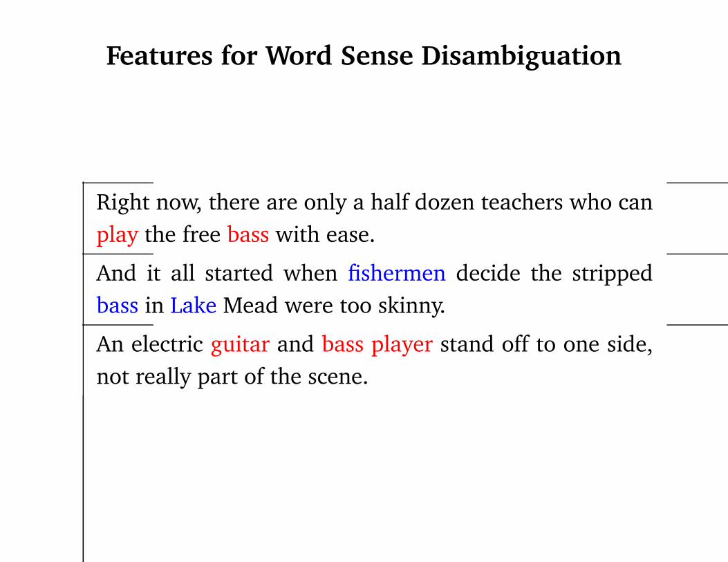
Features for Word Sense Disambiguation

Right now, there are only a half dozen teachers who can

play the free bass with ease.

And it all started when fishermen decide the stripped

bass in Lake Mead were too skinny.

An electric guitar and bass player stand off to one side,

not really part of the scene.

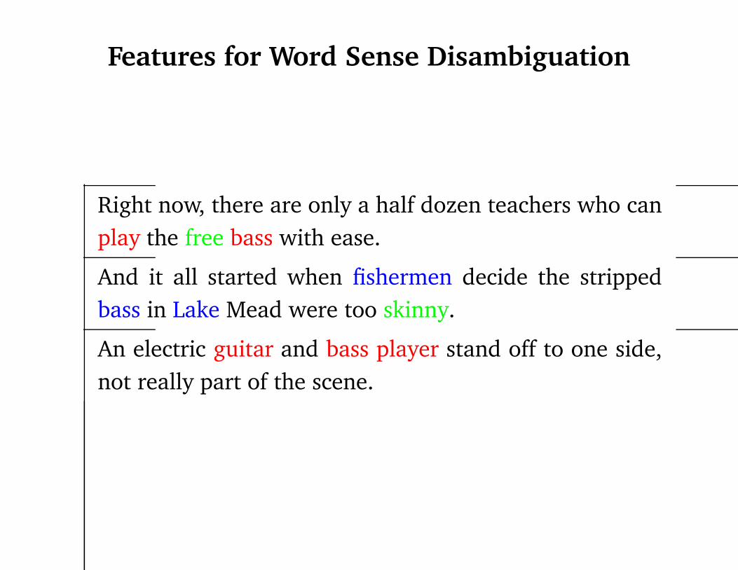
Features for Word Sense Disambiguation

Right now, there are only a half dozen teachers who can

play the free bass with ease.

And it all started when fishermen decide the stripped

bass in Lake Mead were too skinny.

An electric guitar and bass player stand off to one side,

not really part of the scene.

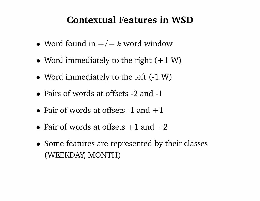
Contextual Features in WSD

• Word found in +/− k word window

• Word immediately to the right (+1 W)

• Word immediately to the left (-1 W)

• Pairs of words at offsets -2 and -1

• Pair of words at offsets -1 and +1

• Pair of words at offsets +1 and +2

• Some features are represented by their classes

(WEEKDAY, MONTH)

Example

The ocean reflects the color of the sky, but even on cloudless days the

color of the ocean is not a consistent blue. Phytoplankton, microscopic

plant life that floats freely in the lighted surface waters, may alter the

color of the water. When a great number of organisms are concen­

trated in an area, . . .

w−1 = microscopic t

−1 =JJ

w+1 = life t+1 =NN

w−2, w

−1 =(Phytoplankton, microscopic) . . .

w−1, w+1 = (microscopic, life)

word-within-k=ocean

word-within-k=reflects

. . .

Decision Lists

• For each feature, we can get an estimate of

conditional probability of sense1 and sense2

• Consider the feature w+1 = life:

Count(plant1, w+1 = life) =100

Count(plant2, w+1 = life) =1

• Maximum-likelihood estimate

P (plant1|w+1 = life) = 100 101

Smoothed Estimates

• Problem: Counts are sparse

Count(plant1, w−1 = P hytoplankton) =2

Count(plant2, w−1 = P hytoplankton) =0

• Solution: Use � smoothing (empirically, � = 0.1 works well):

2 + � P (sense 1 of plant|w−1 = P hytoplankton) =

2 + 2�

100 + � P (sense 1 of plant|w+1 = lif e) =

101 + 2� with � = 0.1, gives values of 0.95 and 0.99 (unsmoothed gives value of 1 and 0.99)

Creating Decision Lists

• For each feature, find

sense(f eature) = argmaxsenseP (sense|f eature)

e.g., sense(w+1 = lif e) = sense1

• Create a rule f eature ∗ sense(f eature) with

weight P (sense(f eature)|f eature)

Rule Weight

w+1 = lif e ∗ plant1 0.99

w+1 = work ∗ plant2 0.93

Creating Decision Lists

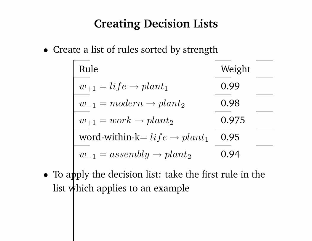
• Create a list of rules sorted by strength

Rule

w+1 = lif e ∗ plant1

w−1 = modern ∗ plant2

w+1 = work ∗ plant2

word-within-k= lif e ∗ plant1

w−1 = assembly ∗ plant2

Weight

0.99

0.98

0.975

0.95

0.94

• To apply the decision list: take the first rule in the

list which applies to an example

Applying Decision ListsThe ocean reflects the color of the sky, but even on cloudless days the color of the ocean is not a consistent blue. Phytoplankton, microscopic plant life that floats freely in the lighted surface waters, may alter the color of the water. When a great number of organisms are concentrated in an area, . . .

Feature

w−1 = microscopic

w+1 = life

w−2 , w−1 =

word-within-k=reflects

. . .

Sense

1

1

N/A

2

Strength

0.95

0.99

0.65

N/A � feature has not seen in training data

w+1 = life � Sense1 is chosen

Experimental Results: WSD

(Yarowsky, 1995)

• Accuracy of 95% on binary WSD

plant

tank

poach

palm

living/factory

vehicle/container

steal/boil

tree/hand

• Accent restoration in Spanish and French — 99%

– useful for restoring accents in de-accented texts, or in automatic generation of accents while typing

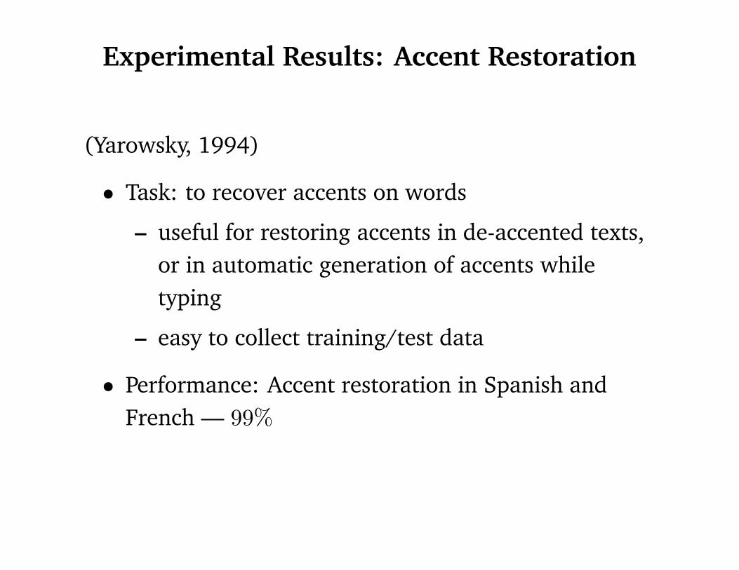
Experimental Results: Accent Restoration

(Yarowsky, 1994)

• Task: to recover accents on words

– useful for restoring accents in de-accented texts,

or in automatic generation of accents while

typing

– easy to collect training/test data

• Performance: Accent restoration in Spanish and

French — 99%

Automatic WSD

• A supervised method: decision lists

• A partially supervised method

• Unsupervised approaches

Beyond Supervised Methods

• If you want to be able to do WSD in the large, you

need to be able to disambiguate all words in a text

• It is hard to get a large amount of annotated data

for every word in a text

– Use existing manually tagged data (SENSEVAL-2,

5000 words from Penn Treebank)

– Use parallel bilingual data

– Check OpenMind Word Expert project

We want unsupervised method for WSD

http://www.openmind.org/

Local Constraints

One sense per collocation: a word reoccurring in

collocation with the same word will almost surely have

the same sense

• That’s why decision list can make accurate

predictions based on the value of just one feature

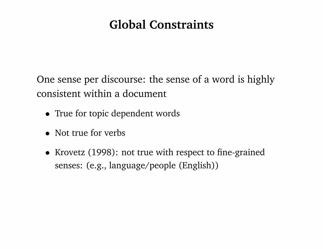
Global Constraints

One sense per discourse: the sense of a word is highly

consistent within a document

• True for topic dependent words

• Not true for verbs

• Krovetz (1998): not true with respect to fine-grained

senses: (e.g., language/people (English))

One sense per discourse

Tested on 37, 232 hand tagged examples

Word

plant

space

tank

bass

crane

Sense

living/factory

volume/outer

vehicle/container

fish/music

bird/machine

Accuracy

99.8%

99.2%

99.6%

100.0%

100.0%

Applicability

72.8%

66.2%

50.5%

58.8%

49.1.0

Semi-Supervised Methods

• Words can be disambiguated based on collocational

features

• Words can be disambiguated based on “one sense

per collocation” constraint

We can take advantage of this redundancy

Bootstrapping Approach

A A A

A A

A A

B B B

B B B

? ??

? ?

?

? ?

?

?

?

? ?

? ?

?

? ? ?

? ?

?

?

? ?

?

?

? ?

? ?

? ??

?

? ?

?? ?

? ?

? ?

??

?

? ? ?

?? ?

?

? ?? ?

?? ? ?

? ?

?

?

??

life

Automatic B B

? ?

? ?

Bootstrapping Approach

A A A

A A

A A

B B B

B B B

? ??

? ?

?

? ?

?

?

?

? ?

? ?

? ?

? ?

?

??

? ?

? ??

?

? ?

?? ?

? ?

? ?

?

?

? ? ?

?

?

? ?? ?

?? ? ?

?

life

Automatic

A A

A

A A

A A

Miscroscopic

Animal

BB B B

BB

Employee

Men B B

? ?

B B

Bootstrapping Approach

A A A

A A

A A

B B B

B B B

?

?

?

?

A A

A

A A

A A

BB B B

BB

Employee

AA A

AA A A

A

A

A

A

A A

A

AAA

AA

A A AA

AA

A A

B BB

BB B

B

B

B B

BB

B BB

B B

BB B B B

B B B

B B

B B

Collecting Seed Examples

• Goal: start with a small subset of the training data

being labeled

– Label a number of training examples by hand

– Pick a single feature for each class by hand

– Use words in dictionary definitions

a vegetable organism, ready for planting or lately

planned

equipment, machinery, apparatus, for industrial

activity

Collecting Seed Examples: An example

• For the “plant” sense distinction, initial seeds are

“word-within-k=life” and

“word-within-k=manufacturing”

• Partition the unlabeled data into three sets:

– 82 examples labeled with “life” sense

– 106 examples labeled with “manufacturing”

sense

– 7350 unlabeled examples

Training New Rules

• From the seed data, learn a decision list of all rules

with weight above some threshold (e.g., all rules

with weight > 0.97)

• Using the new rules, relabel the data (thus,

increasing the amount of annotated examples)

• Induce a new set of rules with weight above the

threshold from the labeled data

• If some examples are still not labeled, return to step

2

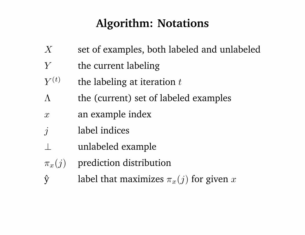
Algorithm: Notations

X set of examples, both labeled and unlabeled

Y the current labeling

Y (t) the labeling at iteration t

� the (current) set of labeled examples

x an example index

j label indices

� unlabeled example

�x(j) prediction distribution

ˆ label that maximizes �x(j) for given xy

=�}

�

�

Algorithm(1) Given:examples X, and initial labeling Y (0)

(2) For t � {0, 1, . . .} (2.1)Train classifier on labeled examples (�(t), Y (t)),

where �(t) = {x � X|Y (t) ⊥

The resulting classifier predicts label j for example x

with probability �(t+1)(j)x

(2.2)For each example x � X :

(2.2.1) Set y = argmaxj �(t+1)

(j)x

(2.2.2) Set

Y (0) if x � �(0)

⎧� x

Yx (t+1)

= ˆ if �(t+1)(ˆy x y) > �

⎧� otherwise

(2.3) If Y (t+1) = Y (t), stop

Experiments

• Baseline score for just picking the most frequent

sense for each word

• Fully supervised method

• Unsupervised Method (based on contextual

clustering)

Results

Word

plant

space

tank

bass

crane

Sense

living/factory

volume/outer

vehicle/container

fish/music

bird/machine

Samp.

7538

5745

11420

1859

2145

Major

53.1

50.7

58.2

56.1

78.0

Superv.

97.7

93.9

97.1

97.8

96.6

Unsuperv.

98.6

93.6

96.5

98.8

95.5

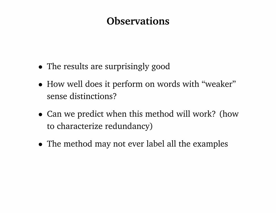
Observations

• The results are surprisingly good

• How well does it perform on words with “weaker”

sense distinctions?

• Can we predict when this method will work? (how

to characterize redundancy)

• The method may not ever label all the examples

Other Applications of Co-training

• Named entity classification (Person, Company,

Location)

. . ., says Dina Katabi, an assistant professor . . .

Spelling features: Full-String=Dina Katabi, Contains(Dina)

Contextual features: appositive=professor

• Web page classification

Words on the page

Pages linking to the page

Two Assumptions Behind Co-training

• Either view is sufficient for learning

There are functions F1 and F2 such that

F (x) = F1(x1) = F2 (x2) = y

for all (x, y) pairs

• Some notion of independence between the two

views

e.g.The Conditional-independence-given-label assumption:

If D(x1, x2, y) is the distribution over examples, then

D(x1, x2, y) = D0(y)D1(x1|y)D2(x2|y)

for some distributions D0, D1 and D2

Rote Learning, and a Graph Interpretation

• In a rote learner, functions F1 and F2 are look-up

tables

Spelling

IBM

Lee

. . .

Category

COMPANY

PERSON

. . .

Context

firm-in

Prof.

. . .

Category

LOCATION

PERSON

. . .

• Note: no chance to learn generalizations such as

“any name containing Alice is a person”

Rote Learning, and a Graph Interpretation

• Each node in the graph is a spelling or context

(A node for IBM, Lee, firm-in, Prof.)

• Each pair (x1i , x2i) is an edge in the graph

(e.g., (Prof. Lee))

• An edge between two nodes mean they have the same

label

(assumption 1: each view is sufficient for classification)

• As quantity of unlabeled data increases, graph becomes

more connected

(assumption 2: some independence between two views)

Automatic WSD

• A supervised method: decision lists

• A partially supervised method

• Unsupervised approaches

Graph-based WSD

• Previous approaches disambiguate each word in

isolation

• Connections between words in a sentence can help

in disambiguation

• Graph is a natural way to capture connections

between entities

We will apply a graph-based approach to WSD, utilizing

relations between senses of various words

Graph-based Representation

• Given a sequence of words W = {w1, . . . , wn}, and

a set of admissible labels for each word NwiLwi = {l1 , . . . , l wi }wi

• Define a weighted graph G(V,E) such that

– V - set of nodes in the graph, where each node

corresponds to a word/label assignment lj wi

– E - set of weighted edges that capture

dependencies between labels

4

Example of Constructed Graph

w1

l w 3

l w 3

l 3

l w 3

l w 3

l w 3

l w 3

l w 3

l 3

2

2

w2

3

3

3 w4

4

4

WW1

3 w1 2

l

l

1 w1

l

W2W3

Construction of Dependency Graph

for i = 1 to N do

for j = i + 1 to N do

for j − i > M axDist then

break

for t = 1 to Nwi do

for s = 1 to Nwj do

weight � Dependency(lt , ls , wi, wj )wi wi

if weight > 0 then

AddEdge(G, lt , ls , weight)wi wi

Ranking Vertices and Label Assignment

Out(v) out-degree of v

d dumping factor

Vertice Ranking

repeat

for all v ⊥ V do ⎨ P (q)P (v) = (1− d) + d � (v,q)�E Out(q)

until convergence of scores P (v)

Label Assignment

for i = 1 to N do

lwi wi � argmax {P (lt )|t = 1 . . . N}

Computing Scores

• For data annotated with sense information, compute

co-occurence statistics or sense n-grams

• For un-annotated data, compute co-occurence

statistics from word glosses in WordNet

snake1 limbless scaly elongate reptile; some are venomous

snake2 a deceitful or treacherous person

crocodile1 large voracious aquatic reptile having a long snout with

massive jaws and sharp teeth

Results

Random select a sense at random

Lesk find senses maximizing overlap in definitions

Random 37.9%

Lesk 48.7%

Graph-based 54.2%

Unsupervised Sense Reranking

• The distribution of word senses is skewed

• Selecting most common sense often produces correct

results

• In WordNet, senses are ordered according to their

frequency in the manually tagged SemCor

– SemCor is small (250,000)

for “tiger” “audacious person” comes before its sense as

“carnivorous animal”

– Most common sense is a domain-dependent notion

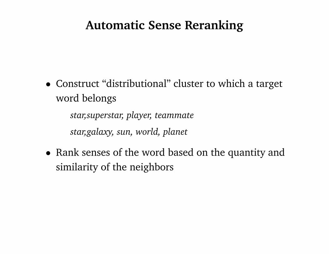
Automatic Sense Reranking

• Construct “distributional” cluster to which a target

word belongs

star,superstar, player, teammate

star,galaxy, sun, world, planet

• Rank senses of the word based on the quantity and

similarity of the neighbors

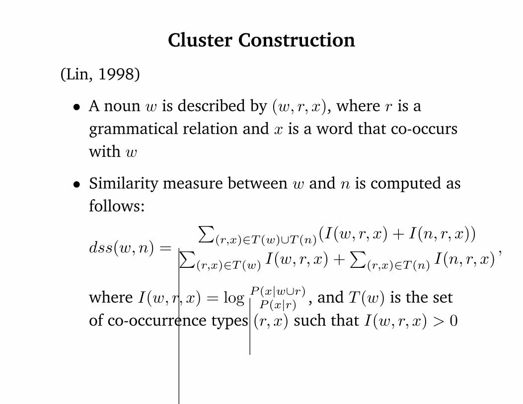
Cluster Construction

(Lin, 1998)

• A noun w is described by (w, r, x), where r is agrammatical relation and x is a word that co-occurswith w

• Similarity measure between w and n is computed asfollows:

⎨(r,x)�T (w)�T (n)(I(w, r, x) + I(n, r, x))

dss(w, n) = ⎨ ⎨ , (r,x)�T (w) I(w, r, x) + (r,x)�T (n) I(n, r, x)

where I(w, r, x) = log P (x|w�r) , and T (w) is the set

P (x|r)

of co-occurrence types (r, x) such that I(w, r, x) > 0

Cluster Ranking

• Let {n1, n2 , . . . , nk } be top k neighbors with associated

distributional similarity

Mw = {dss(w1, n1 ), dss(w2, n2), . . . , dss(wk , nk )}

• Each sense is ranked by summing over the dss(w, nj ) of

each neighbor multiplied by a similarity weight

• Similarity is a weight between the target sense (wsi ) and

the sense of nj that maximizes the score

– counts number of overlapping words in glosses

Evaluation

SemCor predominant sense from manually annotated data

SENSEVAL-2 predominant sense from the test set

precision recall

Automatic 64 63

SemCor 69 68

92 72SENSEVAL-2