disagreement in consumer inflation expectations · disagreement in consumer inflation expectations...

NBP Working Paper No. 278

Disagreement in consumer inflation expectations

Tomasz Łyziak, Xuguang Simon Sheng

Economic Research DepartmentWarsaw, 2018

NBP Working Paper No. 278

Disagreement in consumer inflation expectations

Tomasz Łyziak, Xuguang Simon Sheng

Published by: Narodowy Bank Polski Education & Publishing Department ul. Świętokrzyska 11/21 00-919 Warszawa, Poland www.nbp.pl

ISSN 2084-624X

© Copyright Narodowy Bank Polski, 2018

Tomasz Łyziak – Narodowy Bank PolskiXuguang Simon Sheng – American University

The views expressed in this paper are those of the authors and do not necessarily reflect opinions of the institutions to which they are affiliated.

3NBP Working Paper No. 278

ContentsAbstract 41 Introduction 52 Data and Stylized Facts 9

2.1 Data 92.2 Stylized Facts 11

3 A Model of Consumer Inflation Expectation 134 Empirical Estimation 165 Conclusion 19References 20Appendix 24

Disagreement in Consumer Inflation Expectations

Tomasz Łyziak, Narodowy Bank Polski

Xuguang Simon Sheng, American University

Abstract

We posit that consumers form expectations about inflation by combining two sources ofinformation: their beliefs from shopping experience and news about inflation they learnfrom experts. Disagreement among consumers in our model comes from four sources:(i) consumers’ divergent prior beliefs, (ii) heterogeneity in their propensities to learnfrom experts, (iii) experts’ different views about future inflation, and (iv) difference inmean expectations between consumers and experts. By carefully matching the datasetsfrom the Michigan Survey of Consumers with the Survey of Professional Forecasters,we find that inflation expectations between households and experts differ substantiallyand persistently from each other, and households pay close attention to salient pricechanges, while experts respond more to monetary policy and macro indicators. Ourempirical estimates imply economically significant degrees of information rigidity andthese estimates vary substantially across households. This significant heterogeneityposes a great challenge for the canonical sticky-information model that assumes asingle rate of information acquisition and for noisy-information model in which allagents place the same weight on new information received.

JEL classification: E32; E52Keywords: Consumers, Disagreement, Inflation Expectation, Noisy Information,Sticky Information

Narodowy Bank Polski4

Abstract

1 Introduction

Disagreement about expectations is itself an interesting variable for students of monetary

policy and the business cycle. [...] Disagreement may be a key to macroeconomic dynamics.

N. Gregory Mankiw, Ricardo Reis, and Justin Wolfers, NBER Macroeconomics Annual 2003.

Disagreement about expectations of the public matters. Recent work on macroeconomics

has emphasized the role of disagreement in signaling upcoming structural changes in the

economy (Mankiw, Reis and Wolfers, 2004), and as a proxy for uncertainty in driving business

cycle fluctuations (Bachmann, Elstner and Sims, 2013). Yet why ordinary people disagree

in their expectations, and how best to model this heterogeneity, remains an open question.

We answer this question by matching household and expert inflation expectations and by

building a theory of consumer expectation updating.

Our theory has three key elements. First, consumers hold different beliefs about price

levels, gained from personal experiences on shopping and the previous inflation rates ex-

perienced in their lifetime. Second, consumers obtain public information from experts via

newspapers and social media about the trends in future inflation. Third, households have

different propensities to learn from experts. Consumers then combine public and private

information in forming their inflation expectations. Disagreement among consumers in our

model comes from four sources: (i) consumers’ divergent prior beliefs, (ii) heterogeneity in

their propensities to learn from experts, (iii) experts’ different views about future inflation,

and (iv) deviation of consumer mean expectation from that of experts.

The ingredients of our theory are motivated by the empirical findings. Our primary

database of household forecasts comes from the Michigan Survey of Consumers that con-

tains both quantitative and qualitative inflation expectations. We use both forms of expec-

tations to estimate the central tendency and dispersion among consumers and in particular,

quantify the qualitative responses following the probability method. By carefully matching

Disagreement in Consumer Inflation Expectations

Tomasz Łyziak, Narodowy Bank Polski

Xuguang Simon Sheng, American University

Abstract

We posit that consumers form expectations about inflation by combining two sources ofinformation: their beliefs from shopping experience and news about inflation they learnfrom experts. Disagreement among consumers in our model comes from four sources:(i) consumers’ divergent prior beliefs, (ii) heterogeneity in their propensities to learnfrom experts, (iii) experts’ different views about future inflation, and (iv) difference inmean expectations between consumers and experts. By carefully matching the datasetsfrom the Michigan Survey of Consumers with the Survey of Professional Forecasters,we find that inflation expectations between households and experts differ substantiallyand persistently from each other, and households pay close attention to salient pricechanges, while experts respond more to monetary policy and macro indicators. Ourempirical estimates imply economically significant degrees of information rigidity andthese estimates vary substantially across households. This significant heterogeneityposes a great challenge for the canonical sticky-information model that assumes asingle rate of information acquisition and for noisy-information model in which allagents place the same weight on new information received.

JEL classification: E32; E52Keywords: Consumers, Disagreement, Inflation Expectation, Noisy Information,Sticky Information


Chapter 1

the database of consumer expectations with those of experts from U.S. Survey of Profes-

sional Forecasters, we find that inflation expectations between laymen and experts differ

substantially and persistently from each other. We also observe substantially higher levels

of disagreement among the public than among professional forecasters. Finally, we see that

households pay close attention to salient price changes, such as oil and food prices; see, e.g.

Coibion and Gorodnichenko (2015b), Berge (2017) and Binder (2017b). By contrast, experts

respond more to monetary policy and macro indicators.

Our model is closely related to the theoretical literature on expectations formation with

information frictions. For instance, Mankiw and Reis (2002) propose the sticky information

model that explains agents’ rational inattention in terms of limited resources and the cost of

updating information sets. Carroll (2003) develops an epidemiological model of expectations

formation that can be viewed as providing microfoundations for the Mankiw-Reis model.

Our model differs from the sticky-information model in an important aspect. Disagreement

in Carroll (2003)’s model, or in sticky-information model in general, arises only from different

generations of consumers using different information vintages and there is no disagreement

within a generation. In contrast, our model generates disagreement within a generation due

to consumers’ exposure to different expert views about inflation even under full information

updating. Sims (2003), Woodford (2003) and Maćkowiak and Wiederholt (2009) advocate

the noisy information model that emphasizes the limited ability of economic agents to process

new information from noisy signals. In contrast to the noisy-information model where agents

always solve a signal extraction problem, households in our model observe different views

of experts and use these views as direct inputs in their expectation formation process. The

intuition is straightforward. Ordinary people do not know the latest economic statistics, nor

understand basic economic theory to interpret the data. Observing views of different experts

via newspaper and social media is therefore an important public source of information about

inflation in the future.


Our empirical estimates show that, on average, the propensity for consumers to learn

from experts is about 0.15, implying economically significant degrees of information rigidity

among the public. This magnitude is broadly similar to those reported in the literature

on expectation formation with information frictions. For example, the average estimate of

information rigidity in our dataset, 0.85, is close to the 0.82 value estimated by Coibion and

Gorodnichenko (2012) but is slightly higher than the 0.75 value assumed by Mankiw and

Reis (2002), the 0.75 value calibrated by Hur and Kim (2017) and the 0.73 value estimated

by Carroll (2003). In contrast to all these papers, we also find substantial variations in the

estimated degrees of information rigidity, with attentive consumers revising forecasts very

often, while inattentive consumers making revisions only infrequently. As long as there is

no substantial evidence that would dramatically surprise those inattentive consumers, they

will not revise their previous forecasts, consistent with the so-called predisposition effects

(Branch, 2004). This significant heterogeneity is consistent with the findings in Pfajfar and

Santoro (2013) that consumers split in the two categories – those adjusting their forecasts

toward and away from the professional forecasters’ mean expectation. However, this notable

heterogeneity cannot be explained by the canonical sticky-information model that assumes

a single rate of information acquisition for all agents, nor by the classical noisy-information

model in which all agents place the same weight on new information received.1

Finally, our paper builds on the burgeoning literature exploring cross-sectional distribu-

tion of forecasts. One strand of the literature examines the disagreement among professional

forecasters; see, e.g. Lahiri and Sheng (2008), Capistran and Timmermann (2009), Pat-

ton and Timmermann (2010), Dovern, Fritsche and Slacalek (2012), Andrade and Le Bihan1Mankiw and Reis (2007) and Hur and Kim (2017) generalize the partial equilibrium model with sticky

information to a general equilibrium model and find that information stickiness is present in all markets, andis especially pronounced for consumers. Coibion and Gorodnichenko (2015a) extend the noisy informationmodel by allowing agents to have different signal-noise ratios and therefore placing different weights on thenew information.


Introduction

(2013), Dovern (2015) and Andrade, et al. (2016).2 In contrast to these studies, our paper

focuses on the disagreement among household expectations and is more closely related to a

second strand of literature relying on consumer and business surveys to explore heterogeneity

in expectations. For example, household inflation expectations from the Michigan Survey

of Consumers are found to vary by gender, education levels, or age cohorts (Souleles, 2004;

Bruine de Bruin, et al., 2010; Malmendier and Nagel, 2016). Branch (2004, 2007) estimate

a model in which consumers rationally choose from a set of predictors by evaluating costs

and benefits of each predictor and find that such a model is consistent with the response

behavior of consumers. Lamla and Maag (2012) build a Bayesian learning model and find

that disagreement among consumers (but not professionals) is governed by the amount, the

heterogeneity, and the tone of media reports about consumer price inflation. Dräger and

Lamla (2017) explore disagreement among the general pubic in a multivariate context and

find that disagreement on the interest rate is mainly driven by disagreement on inflation.

The basic structure of our model is similar to Lamla and Maag (2012), but differs in two

important aspects. (i) Consumers in our model observe and directly use experts’ views about

inflation in forming their expectations, rather than proactively estimating the rational fore-

cast of inflation from noisy signals reported in the media. This assumption is supported

by the evidence collected from dozens of surveys from the 1950s to 2014 in Binder (2017a)

that exposes a lack of public awareness of the Federal Reserve and its objectives, a decline2Using expert forecasts from Consensus Economics, Lahiri and Sheng (2008) find that differential in-

terpretation of public information explains most of forecast disagreement as forecast horizon gets shorter;Patton and Timmermann (2010) emphasize the role of heterogeneity in priors in explaining disagreement;and Dovern, Fritsche and Slacalek (2012) investigate determinants of disagreement about six key economicindicators in G7 countries. Using inflation forecasts from U.S. Survey of Professional Forecasters (SPF),Capistran and Timmermann (2009) offer a simple explanation of disagreement based on asymmetries in theforecasters’ costs of over- and underpredicting inflation. Using the ECB SPF forecasts at the micro level,Andrade and Le Bihan (2013) document two new facts – forecasters fail to systematically update their fore-casts and disagree even when updating and accordingly build a hybrid sticky-noisy information model aimedat matching these facts. However, they find that their model cannot quantitatively replicate the error anddisagreement observed in the data. Dovern (2015) and Andrade, et al. (2016) analyze forecast disagreementin a multivariate context.


in public opinion of central bankers, and reasons for consumers’ inattention to monetary

policy. (ii) Rather than the reduced-form estimation of model implications, we perform the

structural estimation that allows us to gauge the relative importance of each channel in

explaining household disagreement in their inflation expectations.

The rest of the paper is organized as follows. Section 2 discusses the dataset from

U.S. Survey of Professional Forecasters and Michigan Survey of Consumers and presents the

stylized facts about consumer inflation expectations. Section 3 proposes a model of consumer

expectation updating. Section 4 provides empirical estimation of the model and section 5

concludes.

2 Data and Stylized Facts

2.1 Data

In our study we analyze short-term inflation expectations of consumers and professional fore-

casters in the United States, formed in a one-year horizon. As far as professional forecasters

are concerned, we use their inflation forecasts reported in the Survey of Professional Forecast-

ers (SPF), conducted by the Philadelphia Fed. As the measure of central tendency we use

medians of individual forecasts, while cross-sectional variance is the measure of disagreement

among professional experts.3

In the case of consumers, we make use of two sets of measures of their inflation ex-

pectations based on Michigan Survey of Consumers (MSC) data. The first set relies on

quantitative assessments of consumers concerning expected price developments. Average ex-

pectations are proxied with the median of individual declarations, while the dispersion is

represented by the implied variance transformed on the basis of interquartile range (IQR):3The mean and median forecasts are almost the same for professional forecasters. Our choice of using

the median is driven by household’ forecasts.


Chapter 2

σimpt =

(IQR

1.35

)2. (1)

The above measure of dispersion is less sensitive to outlier observations than a direct cross-

sectional variance of individual responses.

The second set of measures, including the mean and variance of expected inflation, is

based on quantification of qualitative survey data.4 Given percentages of consumers declaring

expected increase of prices (a), stabilization (b) and reduction (c), we use the Carlson-Parkin

(1975) probability method in order to convert qualitative responses into the distribution of

expected inflation. We assume that the expected inflation is normally distributed in the

population, with unknown mean μ and standard deviation σ. In addition, we assume that

expectations of the respondents stating that prices will not change are located around zero,

within the sensitivity interval (−l, l). Consequently, we can express the observed fractions

of respondents a, b and c as the functions of cumulative standard normal distribution F , the

limit of the sensitivity interval l and the mean and standard deviation of the distribution of

expected inflation rate, i.e.:

at = 1 − F

(l − μt

σt

), (2)

bt = F

(l − μt

σt

)− F

(−l − μt

σt

), (3)

ct = F

(l − μt

σt

). (4)

The above equations can be solved simultaneously, yielding the following formulas for the4Drawing on relevant studies from economics, statistics, sociology and psychology, Mokinski, Sheng and

Yang (2015) provide a detailed review of the literature on measuring disagreement in qualitative survey data.


parameters of the distribution of expected inflation:

μt = lF −1 (ct) + F −1 (1 − at)F −1 (ct) − F −1 (1 − at)

, (5)

σt = −l2

F −1 (ct) − F −1 (1 − at). (6)

As can be noticed, both parameters depend on the unknown width of the sensitivity interval

surrounding zero. To estimate the parameter l, we make an additional assumption. Instead

of assuming unbiasedness of inflation expectations, as Carlson and Parkin (1975) did, we

follow Mankiw, Reis and Wolfers (2004). We make use of quantitative measures of consumer

inflation expectations assuming that, on average, the quantified mean of expected inflation

should equal the quantitative declarations, μq:

T∑t=1

μt

T=

T∑t=1

μqt

T. (7)

The above condition implies that:

l =∑T

t=1 μqt∑T

t=1F −1(ct)+F −1(1−at)F −1(ct)−F −1(1−at)

. (8)

The sensitivity interval calculated in this way using the sample 1995-2016 gives an estimate

of l = 1.1%. It suggests that, on average, the expectations of respondents declaring no

change in prices were located in the interval (−1.1%, 1.1%).

2.2 Stylized Facts

Fact 1: Consumers’ inflation expectations differ substantially and persistently from those of

experts.

Figure 1 plots the median MSC consumer and SPF expert inflation expectations. Expert


Data and Stylized Facts

expectations are only weakly correlated with those of households, correlation of about 0.40

with quantitative expectation and of 0.20 with the quantified measure.5 Furthermore, they

show substantial differences – household inflation expectations are lower than those of experts

before 1996, but become larger and more volatile afterwards.

Fact 2: Disagreement among the general public is substantially higher than that among pro-

fessional forecasters.

Figure 2 plots the disagreement among consumers and experts. The former is measured

either with the implied cross-sectional variance of individual responses in the quantitative

survey or with the variance of distribution of expected inflation quantified on the basis of

qualitative survey. The latter is measured as the cross-sectional variance in SPF inflation

expectations. There are much larger levels of disagreement among consumers than exists

among experts. The contemporaneous correlation between consumer and professional dis-

agreement ranges from 0.24 to 0.30, depending on the measure of consumer disagreement

used, implying different drivers for layman and expert disagreement. Indeed, Lamla and

Maag (2012) find that disagreement among consumers, but not professionals, is governed

by the amount, heterogeneity, and tone of media reports about consumer price inflation.

Ehrmann, Eijffinger and Fratzscher (2012) and Binder (2017a) find evidence for a significant

and sizeable effect of central bank transparency on forecast disagreement among profession-

als, but not on disagreement among the general public.

Fact 3: Households pay more attention to salient price changes, while experts respond more

to macro indicators.

To see this, we run regressions of household and expert expectations on a battery of

variables. In both regressions, we add the lagged dependent variable to control for the

persistence of inflation expectations. We include the following five variables, all from FRED5The two series of consumer inflation expectations, i.e. quantitative and quantified, tend to move together,

with a correlation of 0.76.


database: non-farm employment, Federal Funds rate, Consumer Price Index (CPI), CPI food

price away from home (CPI-food-away) and west Texas intermediate spot crude oil price.

Monthly data are converted to quarterly by computing the average level of the variable within

each quarter. For employment, CPI and CPI-food-away, we then calculate the annualized

quarter-over-quarter change as 400 ∗ log( Xt

Xt−1). To make sure that all those variables are

available to economic agents when they make forecasts, we lag all variables by one period

in the regression. Table 1 reports the regression results. Households pay close attention

to salient price changes, such as oil and food prices, while experts respond more to macro

indicators, such as employment and price level in general. In addition, expert inflation

expectations are much more persistent than those of households, as indicated by the large

and highly significant coefficient in the lagged dependent variable for experts. Notably, this

small set of variables can explain the volatility in expert inflation expectations very well

(R2 = 0.948), but only modestly for households, implying the difficulty in explaining and

modeling expectations formation process of ordinary people.

3 A Model of Consumer Inflation Expectation

Imagine that a consumer forms his expectation about inflation in the future. He has access

to two sources of information: (i) private sources of information gained from personal expe-

riences on shopping and pumping at gas stations and (ii) public information gathered from

countless advertisements, news media report and expectations of experts. He then combines

these two types of information to form his inflation expectation. To fix ideas, let Cit be

consumer i’s inflation expectation based on the information available at time t, Pit be expert

i’s inflation expectation at time t, and λi ∈ (0, 1) be consumer i’s propensity to learn from

experts. We consider three different cases.

Case 1: For the moment, we assume that all consumers learn the same news from


Chapter 3

experts, mimicking the “common source” story in epidemiology where people get sick because

of their common exposure to the polluted air in Washington, DC. Consumers have different

propensities to learning and this heterogeneity might reflect democratic characteristics, such

as gender, education levels and age cohorts. In this case, consumer i’s inflation expectation

is the weighted average of the common expert view, Pt and his prior belief, Ci,t−1 as in

equation (9):

Cit = λiPt + (1 − λi)Ci,t−1. (9)

For convenience, we denote x̄t as the cross-sectional average of xit, i.e. x̄t = Ei(xit), and

σ2xt as the cross-sectional variance of xit, i.e. σ2

xt = V ari(xit). Then consumers’ forecast

disagreement, measured by σ2ct, evolves as follows:

σ2ct =

[σ2

λ + (1 − λ̄)2]σ2

c,t−1 + σ2λ(p̄t − c̄t−1)2. (10)

Equation (10) decomposes consumer inflation forecast disagreement into three sources: (i)

heterogeneity in consumers’ prior beliefs, σ2c,t−1, (ii) heterogeneity in their propensities to

learn from experts, σ2λ and (iii) deviation of consumer mean expectation from that of experts,

(p̄t − c̄t−1)2.

Case 2: Now we allow for the possibility that consumers might learn different views about

inflation from different newspapers and social media. Sometimes, even the same newspaper

contains different views about future inflation. In line with Carroll (2003), we assume that

consumers have the same propensity to learn from experts. In this case, consumer i’s inflation

expectation can be described as follows

Cit = λPit + (1 − λ)Ci,t−1. (11)


Equation (11) allows for a simple variance decomposition where the covariance term between

Pit and Ci,t−1 is zero:

σ2ct = (1 − λ)2σ2

c,t−1 + λ2σ2pt. (12)

Forecast disagreement in this case arises from the heterogeneity in consumers’ prior beliefs

and in experts’ divergent views about future inflation. Before we present a more general

model of consumer expectation formation, we need to point out the key differences between

our model and Carroll (2003)’s model. Carroll (2003) assumes that each consumer faces a

constant probability λ of encountering and absorbing the contents of an article on inflation

and that consumers who do not encounter an article simply continue to believe the last

forecast they read about. As such, disagreement in his model arises only from different

generations of consumers using different information vintages and there is no disagreement

within a generation. In contrast, our model generates disagreement within a generation due

to consumers’ exposure to different expert views about inflation even under full information

updating λ = 1.

Case 3: Finally, we relax both assumptions and present a general model of consumer

inflation expectation. In this model, consumers are allowed to have different propensities

to learn from experts who might have different views about future inflation. Consumer i’s

inflation expectation at time t evolves according to the following equation

Cit = λiPit + (1 − λi)Ci,t−1. (13)

Under the assumption that Ci,t−1, λi and Pit are orthogonal to each other, we derive the

dynamics of consumer forecast disagreement as follows6

6The appendix contains details for the derivation.


A Model of Consumer Inflation Expectation

σ2ct =

[σ2

λ + (1 − λ̄)2]σ2

c,t−1 + (σ2λ + λ̄2)σ2

pt + σ2λ(p̄t − c̄t−1)2. (14)

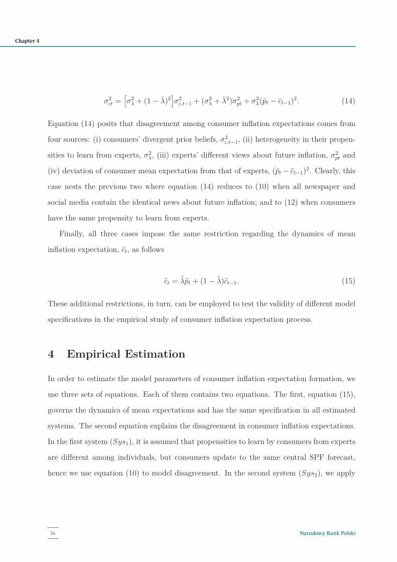
Equation (14) posits that disagreement among consumer inflation expectations comes from

four sources: (i) consumers’ divergent prior beliefs, σ2c,t−1, (ii) heterogeneity in their propen-

sities to learn from experts, σ2λ, (iii) experts’ different views about future inflation, σ2

pt and

(iv) deviation of consumer mean expectation from that of experts, (p̄t − c̄t−1)2. Clearly, this

case nests the previous two where equation (14) reduces to (10) when all newspaper and

social media contain the identical news about future inflation; and to (12) when consumers

have the same propensity to learn from experts.

Finally, all three cases impose the same restriction regarding the dynamics of mean

inflation expectation, c̄t, as follows

c̄t = λ̄p̄t + (1 − λ̄)c̄t−1. (15)

These additional restrictions, in turn, can be employed to test the validity of different model

specifications in the empirical study of consumer inflation expectation process.

4 Empirical Estimation

In order to estimate the model parameters of consumer inflation expectation formation, we

use three sets of equations. Each of them contains two equations. The first, equation (15),

governs the dynamics of mean expectations and has the same specification in all estimated

systems. The second equation explains the disagreement in consumer inflation expectations.

In the first system (Sys1), it is assumed that propensities to learn by consumers from experts

are different among individuals, but consumers update to the same central SPF forecast,

hence we use equation (10) to model disagreement. In the second system (Sys2), we apply


Chapter 4

equation (12), according to which propensities to learn do not differ among consumers,

but consumers update their views to different SPF forecasts. Finally, the third system

(Sys3) exploits equation (14) for disagreement, which reflects the case, in which parameters

λ differ among individuals and consumers update to different SPF forecasts. To allow for

correleted error terms across both equations, we conduct the estmation with the use of

seemingly unrelated regressions (SUR) method. Systems are estimated either with the use

of the outcomes from quantitative survey questions or exploiting the distribution of expected

inflation quantified on the basis of qualitative survey data.

In our estimations we use two sample periods. Both of them start in 1985Q1. The

whole sample ends in 2016Q3, while the shorter sample ends in 2007Q4. Estimation results

based on the whole sample period allow assessing which model for disagreement of consumer

inflation expectations displays the best statistical fit. To make this analysis more robust,

the systems estimated till the end of 2007 are then used to forecast the level and dispersion

of consumer inflation expectations in the 2008-2016. Table 2 presents the estimation results.

We find that the third system of equations (Sys3) is the only one, in which the estimated

parameters are significant in both sample periods, independently of the measures of consumer

inflation expectations. The models for the level of consumer inflation expectations display

a better empirical fit (adj.R2) if the measures of inflation expectations quantified with the

probability method are used instead of quantitative expectations. The opposite conclusion

concerns the models of disagreement in consumer expectations – in this case the measures

based on the responses to the quantitative MSC question are preferred to qualitative ones.

A comparison of empirical fit of individual models does not indicate a single best model for

disagreement. The above mixed results hold both in systems estimated in the whole sample

and in the short sample.

Even if a comparison of coefficients of determination does not indicate the preferred

model, assessment of out-of-sample forecasting accuracy offers more robust conclusions. It


Empirical Estimation

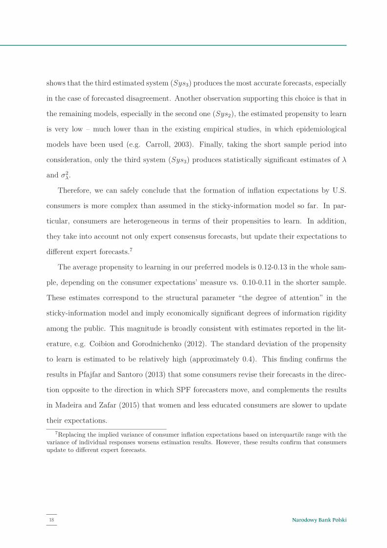
shows that the third estimated system (Sys3) produces the most accurate forecasts, especially

in the case of forecasted disagreement. Another observation supporting this choice is that in

the remaining models, especially in the second one (Sys2), the estimated propensity to learn

is very low – much lower than in the existing empirical studies, in which epidemiological

models have been used (e.g. Carroll, 2003). Finally, taking the short sample period into

consideration, only the third system (Sys3) produces statistically significant estimates of λ

and σ2λ.

Therefore, we can safely conclude that the formation of inflation expectations by U.S.

consumers is more complex than assumed in the sticky-information model so far. In par-

ticular, consumers are heterogeneous in terms of their propensities to learn. In addition,

they take into account not only expert consensus forecasts, but update their expectations to

different expert forecasts.7

The average propensity to learning in our preferred models is 0.12-0.13 in the whole sam-

ple, depending on the consumer expectations’ measure vs. 0.10-0.11 in the shorter sample.

These estimates correspond to the structural parameter “the degree of attention” in the

sticky-information model and imply economically significant degrees of information rigidity

among the public. This magnitude is broadly consistent with estimates reported in the lit-

erature, e.g. Coibion and Gorodnichenko (2012). The standard deviation of the propensity

to learn is estimated to be relatively high (approximately 0.4). This finding confirms the

results in Pfajfar and Santoro (2013) that some consumers revise their forecasts in the direc-

tion opposite to the direction in which SPF forecasters move, and complements the results

in Madeira and Zafar (2015) that women and less educated consumers are slower to update

their expectations.7Replacing the implied variance of consumer inflation expectations based on interquartile range with the

variance of individual responses worsens estimation results. However, these results confirm that consumersupdate to different expert forecasts.


5 Conclusion

By matching the datasets from the Michigan Survey of Consumers with the Survey of Pro-

fessional Forecasters, we find that inflation expectations between households and experts

differ substantially and persistently from each other, and households pay close attention to

salient price changes, while experts responding more to monetary policy and macro indica-

tors. We then build a theory of consumer expectation updating. Our theory has three key

elements. First, consumers hold different beliefs about price levels, gained from personal

experiences on shopping and pumping at gas stations. Second, consumers obtain public in-

formation from experts via newspapers and social media about the trends in future inflation.

Third, households have different propensities to learn from experts. Disagreement among

consumers in our model comes from four sources: (i) consumers’ divergent prior beliefs, (ii)

heterogeneity in their propensities to learn from experts, (iii) experts’ different views about

future inflation, and (iv) deviation of consumer mean expectation from that of experts.

Estimation results suggest that consumers form their inflation expectations in a more

complex manner than assumed in the sticky-information model so far. Propensities to learn-

ing from experts differ among individuals, who update their expectations to forecasts of

different professionals. Therefore all ingredients of our theory seem important in explaining

households inflation expectations.

Our empirical estimates imply economically significant degrees of information rigidity

and these estimates vary substantially across households. This significant heterogeneity

poses a great challenge for the canonical sticky-information model that assumes a single

rate of information acquisition and for noisy-information model in which all agents place the

same weight on new information received. Future research is warranted by incorporating

this notable heterogeneity in information updating into expectations formation process.


Chapter 5

References

Andrade, P. and H. Le Bihan (2013). Inattentive Professional Forecasters. Journal of Mon-

etary Economics 60, 976-982.

Andrade, P., R. Crump, S. Eusepi and E. Moench (2016). Fundamental Disagreement. Jour-

nal of Monetary Economics 83, 106-128.

Bachmann R., S. Elstner and E. Sims (2013). Uncertainty and Economic Activity: Evidence

from Business Survey Data. American Economic Journal: Macroeconomics 5, 217-249.

Berge, T.J. (2017). Understanding Survey Based Inflation Expectations. Federal Reserve

Board working paper 2017-046.

Binder, C.C. (2017a). Fed Speak on Main Street: Central Bank Communication and House-

hold Expectations. Journal of Macroeconomics 52, 238-251.

Binder, C.C. (2017b). Inflation Expectations and the Price at the Pump. Haverford College,

Department of Economics working paper.

Branch, W.A. (2004). The Theory of Rationally Heterogeneous Expectations: Evidence from

Survey Data on Inflation Expectations. Economic Journal 114, 592-621.

Branch, W.A. (2007). Sticky Information and Model Uncertainty in Survey Data on Inflation

Expectations. Journal of Economic Dynamics and Control 31, 245-276.

Bruine de Bruin, W., W. Vanderklaauw, J.S. Downs, B. Fischhoff, G. Topa and O. Armantier

(2010). Expectations of Inflation: The Role of Demographic Variables, Expectation For-

mation, and Financial Literacy. Journal of Consumer Affairs 44(2), 381-402.

Capistran, C. and A. Timmermann (2009). Disagreement and Biases in Inflation Expecta-

tions. Journal of Money, Credit and Banking 41, 365-396.


References

Carlson, J.A. and M.J. Parkin (1975). Inflation Expectations. Economica 42(166), 123-138.

Carroll, C.D. (2003). Macroeconomic Expectations of Households and Professional Forecast-

ers. Quarterly Journal of Economics 118, 269-298.

Coibion, O. (2010). Testing the Sticky Information Phillips Curve. Review of Economics and

Statistics 92(1), 87-101.

Coibion, O. and Y. Gorodnichenko (2012). What can Survey Forecasts Tell us about Infor-

mational Rigidities? Journal of Political Economy 120, 116-159.

Coibion, O. and Y. Gorodnichenko (2015a). Information Rigidity and the Expectations For-

mation Process: A Simple Framework and New Facts. American Economic Review 105,

2644-2678.

Coibion, O. and Y. Gorodnichenko (2015b). Is the Phillips Curve Alive and Well After

All? Inflation Expectations and the Missing Disinflation. American Economic Journal:

Macroeconomics 7(1), 197-232.

Dovern, J., U. Fritsche and J. Slacalek (2012). Disagreement among Professional Forecasters

in G7 Countries. Review of Economics and Statistics 94, 1081-1096.

Dovern, J. (2015). A Multivariate Analysis of Forecast Disagreement: Confronting Models

of Disagreement with Survey Data. European Economic Review 80, 1081-1096.

Dräger, L. and M.J. Lamla (2017). Explaining Disagreement on Interest Rates in a Taylor-

Rule Setting. Scandinavian Journal of Economics 119(4), 987-1009.

Ehrmann, M., S. Eijffinger and M. Fratzscher (2012). The Role of Central Bank Transparency

for Guiding Private Sector Forecasts. Scandinavian Journal of Economics 114(3), 1018-

1052.


References

Hur, J. and I. Kim (2017) Inattentive Agents and Disagreement about Economic Activity.

Economic Modelling 63, 175-190.

Lahiri, K. and X. Sheng (2008). Evolution of Forecast Disagreement in a Bayesian Learning

Model. Journal of Econometrics 144, 325-340.

Lamla, M.J. and T. Maag (2012). The Role of Media for Inflation Forecast Disagreement

of Households and Professional Forecasters. Journal of Money, Credit and Banking 44,

1325-1350.

Maćkowiak, B. and M. Wiederholt (2009). Optimal Sticky Prices under Rational Inattention.

American Economic Review 99, 769-803.

Madeira, C. and B. Zafar (2015). Heterogeneous Inflation Expectations and Learning. Jour-

nal of Money, Credit and Banking 47(5), 867-896.

Malmendier, U. and S. Nagel (2016). Learning from Inflation Experiences. Quarterly Journal

of Economics 131(1), 53-87.

Mankiw, G. and R. Reis (2002). Sticky Information versus Sticky Prices: A Proposal to

Replace the New Keynesian Phillips Curve. Quarterly Journal of Economics 117, 1295-

1328.

Mankiw, G. and R. Reis (2007). Sticky Information in General Equilibrium. Journal of the

European Economic Association 5, 603-613.

Mankiw, N.G., R. Reis and J. Wolfers (2004). Disagreement about Inflation Expectations.

In NBER Macroeconomics Annual 2003, Gertler M. and K. Rogoff (eds). MIT Press,

Cambridge, MA, 209-248.

Mokinski, F., X.S. Sheng and J. Yang (2015). Measuring Disagreement in Qualitative Ex-

pectations. Journal of Forecasting 34, 405-426.


Patton, A.J. and A. Timmermann (2010). Why do Forecasters Disagree? Lessons from the

Term Structure of Cross-sectional Dispersion. Journal of Monetary Economics 57, 803-820.

Pfajfar, D. and E. Santoro (2013). News on Inflation and the Epidemiology of Inflation

Expectations. Journal of Money, Credit and Banking 45(6), 1045-1067.

Sims, C.A. (2003). Implications of Rational Inattention. Journal of Monetary Economics 50,

665-690.

Souleles, N.S. (2004). Expectations, Heterogeneous Forecast Errors, and Consumption: Mi-

cro Evidence from the Michigan Consumer Sentiment Surveys. Journal of Money, Credit

and Banking 36(1), 39-72.

Woodford, M. (2003). Imperfect Common Knowledge and the Effects of Monetary Policy. In

Knowledge, Information, and Expectations in Modern Macroeconomics: In Honor of Ed-

mund Phelps, edited by Aghion, P., R. Frydman, J. Stiglitz and M. Woodford, Princeton,

NJ: Princeton Univ. Press.


References

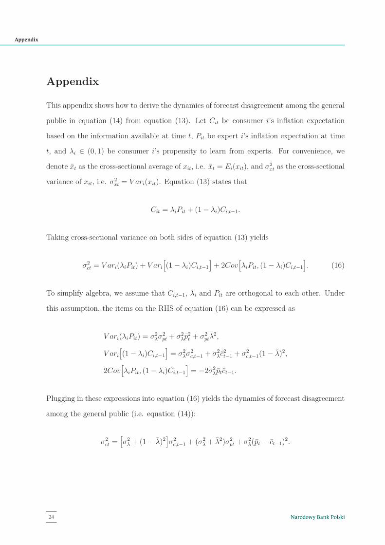
Appendix

This appendix shows how to derive the dynamics of forecast disagreement among the general

public in equation (14) from equation (13). Let Cit be consumer i’s inflation expectation

based on the information available at time t, Pit be expert i’s inflation expectation at time

t, and λi ∈ (0, 1) be consumer i’s propensity to learn from experts. For convenience, we

denote x̄t as the cross-sectional average of xit, i.e. x̄t = Ei(xit), and σ2xt as the cross-sectional

variance of xit, i.e. σ2xt = V ari(xit). Equation (13) states that

Cit = λiPit + (1 − λi)Ci,t−1.

Taking cross-sectional variance on both sides of equation (13) yields

σ2ct = V ari(λiPit) + V ari

[(1 − λi)Ci,t−1

]+ 2Cov

[λiPit, (1 − λi)Ci,t−1

]. (16)

To simplify algebra, we assume that Ci,t−1, λi and Pit are orthogonal to each other. Under

this assumption, the items on the RHS of equation (16) can be expressed as

V ari(λiPit) = σ2λσ2

pt + σ2λp̄2

t + σ2ptλ̄

2,

V ari

[(1 − λi)Ci,t−1

]= σ2

λσ2c,t−1 + σ2

λc̄2t−1 + σ2

c,t−1(1 − λ̄)2,

2Cov[λiPit, (1 − λi)Ci,t−1

]= −2σ2

λp̄tc̄t−1.

Plugging in these expressions into equation (16) yields the dynamics of forecast disagreement

among the general public (i.e. equation (14)):

σ2ct =

[σ2

λ + (1 − λ̄)2]σ2

c,t−1 + (σ2λ + λ̄2)σ2

pt + σ2λ(p̄t − c̄t−1)2.


Appendix

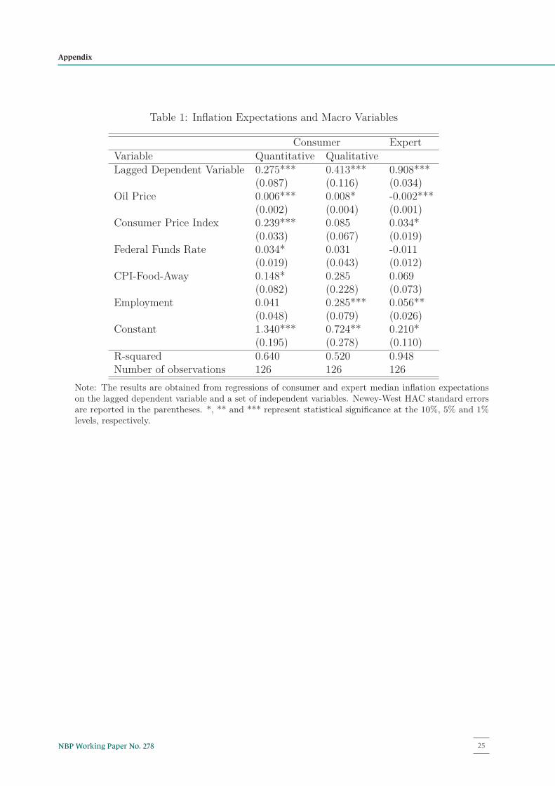
Table 1: Inflation Expectations and Macro Variables

Consumer ExpertVariable Quantitative QualitativeLagged Dependent Variable 0.275*** 0.413*** 0.908***

(0.087) (0.116) (0.034)Oil Price 0.006*** 0.008* -0.002***

(0.002) (0.004) (0.001)Consumer Price Index 0.239*** 0.085 0.034*

(0.033) (0.067) (0.019)Federal Funds Rate 0.034* 0.031 -0.011

(0.019) (0.043) (0.012)CPI-Food-Away 0.148* 0.285 0.069

(0.082) (0.228) (0.073)Employment 0.041 0.285*** 0.056**

(0.048) (0.079) (0.026)Constant 1.340*** 0.724** 0.210*

(0.195) (0.278) (0.110)R-squared 0.640 0.520 0.948Number of observations 126 126 126

Note: The results are obtained from regressions of consumer and expert median inflation expectationson the lagged dependent variable and a set of independent variables. Newey-West HAC standard errorsare reported in the parentheses. *, ** and *** represent statistical significance at the 10%, 5% and 1%levels, respectively.


Appendix

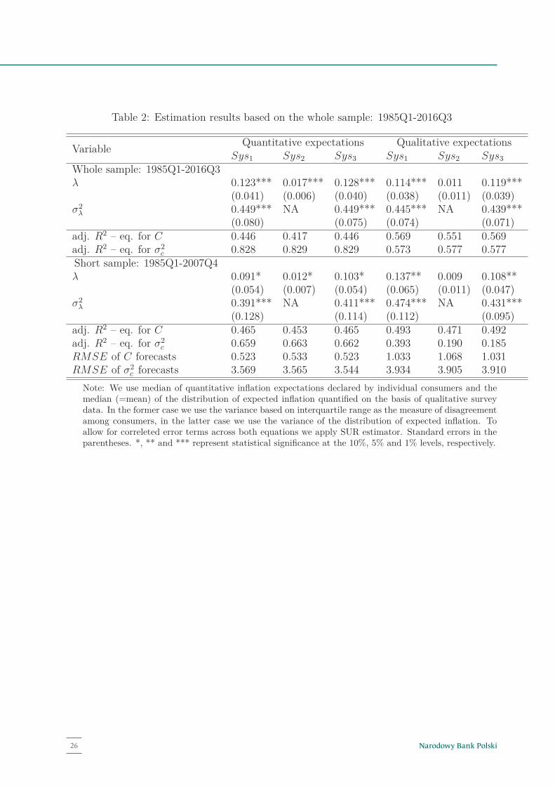
Table 2: Estimation results based on the whole sample: 1985Q1-2016Q3

Variable Quantitative expectations Qualitative expectationsSys1 Sys2 Sys3 Sys1 Sys2 Sys3

Whole sample: 1985Q1-2016Q3λ 0.123*** 0.017*** 0.128*** 0.114*** 0.011 0.119***

(0.041) (0.006) (0.040) (0.038) (0.011) (0.039)σ2

λ 0.449*** NA 0.449*** 0.445*** NA 0.439***(0.080) (0.075) (0.074) (0.071)

adj. R2 – eq. for C 0.446 0.417 0.446 0.569 0.551 0.569adj. R2 – eq. for σ2

c 0.828 0.829 0.829 0.573 0.577 0.577Short sample: 1985Q1-2007Q4λ 0.091* 0.012* 0.103* 0.137** 0.009 0.108**

(0.054) (0.007) (0.054) (0.065) (0.011) (0.047)σ2

λ 0.391*** NA 0.411*** 0.474*** NA 0.431***(0.128) (0.114) (0.112) (0.095)

adj. R2 – eq. for C 0.465 0.453 0.465 0.493 0.471 0.492adj. R2 – eq. for σ2

c 0.659 0.663 0.662 0.393 0.190 0.185RMSE of C forecasts 0.523 0.533 0.523 1.033 1.068 1.031RMSE of σ2

c forecasts 3.569 3.565 3.544 3.934 3.905 3.910Note: We use median of quantitative inflation expectations declared by individual consumers and themedian (=mean) of the distribution of expected inflation quantified on the basis of qualitative surveydata. In the former case we use the variance based on interquartile range as the measure of disagreementamong consumers, in the latter case we use the variance of the distribution of expected inflation. Toallow for correleted error terms across both equations we apply SUR estimator. Standard errors in theparentheses. *, ** and *** represent statistical significance at the 10%, 5% and 1% levels, respectively.


Figure 1: Median Inflation Expectations: MSC Consumers vs. SPF Experts


Appendix

Figure 2: Disagreement among consumers and forecasters


www.nbp.pl

disagreement in consumer inflation expectations · disagreement in consumer inflation expectations...

Documents