disaggregated approaches to freight analysis: a...
TRANSCRIPT
This is a repository copy of Disaggregated Approaches to Freight Analysis: A Feasibility Study..
White Rose Research Online URL for this paper:http://eprints.whiterose.ac.uk/2176/
Monograph:Fowkes, A.S., Nash, C.A., Toner, J.P. et al. (1 more author) (1993) Disaggregated Approaches to Freight Analysis: A Feasibility Study. Working Paper. Institute of Transport Studies, University of Leeds , Leeds, UK.
Working Paper 399
[email protected]://eprints.whiterose.ac.uk/
Reuse See Attached
Takedown If you consider content in White Rose Research Online to be in breach of UK law, please notify us by emailing [email protected] including the URL of the record and the reason for the withdrawal request.
White Rose Research Online
http://eprints.whiterose.ac.uk/
Institute of Transport StudiesUniversity of Leeds
This is an ITS Working Paper produced and published by the University of Leeds. ITS Working Papers are intended to provide information and encourage discussion on a topic in advance of formal publication. They represent only the views of the authors, and do not necessarily reflect the views or approval of the sponsors. White Rose Repository URL for this paper: http://eprints.whiterose.ac.uk/2176/
Published paper Fowkes, A.S., Nash, C.A., Toner, J.P., Tweddle, G. (1993) Disaggregated Approaches to Freight Analysis: A Feasibility Study. Institute of Transport Studies, University of Leeds. Working Paper 399
White Rose Consortium ePrints Repository [email protected]
UNIVERSITY OF LEEDS
Institute for Transport Studies
ITS Working Paper 399 ISSN 0142-8942
June 1993
DISAGGREGATED APPROACHES TO FREIGHT ANALYSIS: A FEASIBILTIY STUDY
AS Fowkes
CA Nash
JP Toner
G Tweddle
ITS Working Papers are intended to provide information and encourage discussion on a topic in
advance of formal publication. They represent only the views of the authors, and do not
necessarily reflect the views or approval of the sponsors.
This work was sponsored by the Department of Transport, London.

CONTENTS
Page
PREFACE
1. INTRODUCTION AND BACKGROUND 1
1.1Introduction 1
1.2Methodology and outline of the report 2
1.3Brief overview 4
2. DATA SOURCES 9
2.1Introduction 9
2.2Transport statistics 9
2.3Industrial output data and forecasts 10
2.4Availability of consistent data over time 11
3. MACROECONOMIC FORECASTING MODELS 12
4. ECONOMETRIC MODELS OF DEMAND FOR
ROAD FREIGHT TRANSPORT 15
4.1Introduction 15
4.2Data 15
4.3Econometric issues 16
4.4Results of regressions on sectoral output and gross domestic product 17
4.4.1Agriculture and foodstuffs (NST 0 + 1) 22
4.4.2Crude materials (NST 04) 22
4.4.3Wood, timber and cork (NST 05) 22
4.4.4Coal and coke (NST 2) 22
4.4.5Petroleum and oil product (NST 3) 22
4.4.6Ores (NST 4) 22
4.4.7Iron and steel products (NST 5) 23
4.4.8Crude minerals (NST 6) 23
4.4.9Cement and lime (NST 64) 23
4.4.10Fertilisers (NST 7) 23
4.4.11Chemicals (NST 8) 23
4.4.12Transport, equipment and machinery (NST 91-93) 23
4.4.13Manufacturers of metal (NST 94) 23
4.4.14Miscellaneous manufactures (NST 96-7) 24
4.4.15Miscellaneous articles (NST 98-99) 24
4.4.16Whole economy 24
4.5Use of the models for forecasting 24
4.6Conclusions 25
5. HANDLING FACTORS AND LENGTH OF HAUL 45
5.1Handling factors of commodities 45
5.2Linking length of haul and handling factors 48
(ALL MODES)

6. CHANGES IN ROAD DISTRIBUTION PATTERNS
AND THE DEMANDS OF USERS 53
6.1The overall position 53
6.2Food, drink and tobacco (NST 0 and NST 1, excluding 04, 05 and 09) 53
6.3Crude minerals (NST 04, 09, 84) 54
6.4Wood, timber and cork (NST 05) 56
6.5Coal and coke (NST 21-23) 56
6.6Petrol & petroleum products (NST 31-34, 83) 56
6.7Ores (NST 41, 45, 46) 56
6.8Iron and steel products (NST 51-56. Pig iron, crude steel
(sheets bars etc), unwrought and non-ferrous alloys) 57
6.9Crude minerals (NST 6 excluding 64 and 69) 57
6.10Cements and other building materials (NST cement & lime 64.
Other building materials (brick etc, concrete, glass and pottery) 69, 95) 57
6.11Fertilisers (NST 71, 72) 57
6.12Chemicals (NST 81, 82, 89) 58
6.13Machinery and transport equipment (NST 91-93. Vehicles, tractors,
electrical and non-electrical machines) 58
6.14Other metal products, nes (NST 94 Structural parts etc) 58
6.15Miscellaneous manufactures (NST 96, 97. Leather, textiles
and clothing nes) 59
6.16Miscellaneous articles (NST 98, 99. Arms, ammunition, commodities
nes and unknown commodoties) 59
6.17Future trends 59
7. CHANGES IN VEHICLES AND VEHICLE ACTIVITY 60
7.1Effect of legislative changes 60
7.2Forthcoming legislative changes 63
7.3Effect of the transport environment 64
7.4Vehicle stock and replacement 65
7.5Pressure for change in vehicle usage 77
8. THE USE OF SMALL GOODS VEHICLES 78
8.1Commentary 78
8.2Econometric modelling of the use of small goods vehicles 80
8.3Conclusion 82
9. FREIGHT MODE CHOICE 83
9.1Introduction 83
9.2Development in distribution systems 83
9.3Determinants of freight mode choice 85
9.3.1Introduction 85
9.3.2Survey and modelling methodologies 86
9.3.3Results of the survey 86
9.4Commentary 91
9.4.1Food and drink 91
9.4.2Petroleum products (NST 3) 92
9.4.3Tubes, pipes and fittings (NST 55) 93
9.4.4Cement and lime (NST 64) 93
9.4.5Feritilisers (NST 7) 93
9.4.6Electrical goods (NST 93) 94
9.4.7Pulp, paper and board (NST 841/972/973) 94
9.4.8Container traffic 95
9.5Prospects for modal shift 95
10. OTHER RELEVANT ISSUES 97
10.1Introduction 97
10.2Relevance of port traffic 97
10.3Bulk and semi-bulk traffic 98
10.3.1The major bulks - fuel and iron ore 98
10.3.2Importation versus demestic production 99
10.3.3Semi-bulks 100
10.3.4Container traffic 100
10.3.5Combined traffic 101
10.4Seaborne trades and the effect on inland transport 102
10.5Regional disaggregation of road traffic 103
10.6Changes in the use of categories of roads 106
11. CONCLUSIONS AND RECOMMENDATIONS 107
11.1Overview 107
11.2What decisions are the forecast meant to inform? 108
11.3Findings and recommendation regarding data sources 108
11.4Findings and recommendations regarding modelling 109
11.5The value of disaggregate freight forecasting 110
BIBLIOGRAPHY 111
ANNEX 1 113
ANNEX 2 114

DISAGGREGATED APPROACHES TO FREIGHT ANALYSIS:
A FEASIBILITY STUDY
EXECUTIVE SUMMARY
The Department of Transport has a number of needs for freight forecasts. The dominant one is
as a component of the National Road Traffic Forecasts, which are an essential input into road
infrastructure planning and the examination of future environmental issues. The Department is
also responsible for approval of certain investment projects and other modes of freight transport
such as rail and canal.
The current method used by the Department of Transport to forecast lorry traffic is a simple
`aggregate level' relationship between tonnes-kilometres and GDP. Over the last 15 years this
relationship has been stable and close. The Department has therefore been spared the necessity
of developing and monitoring forecasting models at a disaggregate level, eg. by commodity
sectors. However, there are reasons (discussed below) for believing that better forecasts can be
derived from a disaggregate approach, and in any event the Department has other uses for
disaggregate forecasts. In order to investigate the position further, the Department
commissioned this study as part of its Research Programme on Longer Term Issues. The study
faced many difficulties, particularly the non-availability of promised data sources, but has been
able to reach a firm conclusion, namely that it would be sensible and worthwhile for the
Department to institute a programme of monitoring, modelling and forecasting disaggregated
flows over several key sectors, or groups of sectors.
The supporting evidence set out in the report can be summarised as follows. Firstly, the
proportional relationship between road tonne-kilometres and GDP, on which the Department
currently relies, has no theoretical support. The increase in tonne-kilometres has two
components: an increase in tonnes lifted which is less than proportional to GDP; and a large
concentration of production facilities and a reduction in the number of distribution depots that a
given firm will use to supply the country. Although these trends will no doubt continue, with an
extension of Europe-wide production and distribution systems, we see the future scope for
further movement in these directions to be distinctly less than in the past 15 years. Consequently
we expect the average length of road haul to rise at a slower rate and, since we cannot see any
reason for an offsetting increase in tonnes lifted, we expect the Department's current aggregate
approach to overpredict road tonne kilometres.
Secondly, our investigations into the freight histories of individual commodity groups suggests
that there are important differences in the way they are related to GDP growth. In addition there
are expected to be some cases of large scale restructuring, particularly in relation to the (ex-)
Nationalised Industries. We see no reason why the freight transport implications should be
mutually offsetting, and so doubt the ability of an aggregate model to cope at all well. As a first
attempt at testing this, we have constructed econometric freight demand forecasting models for
15 sectors. While this is probably a greater level of disaggregation than optimum, and some
forecasting equations were particularly poor, our evaluation of the resulting forecasting ability is
that it is preferable to the aggregate model both in terms of providing a closer forecasting for the
next year and in giving a smaller confidence interval about this forecast. In addition, it is clearly
a lot easier to allow for known future changes in particular sectors when using disaggregate
models.
Thirdly, even if the Department's current method had been satisfactory for forecasting tonne-
kilometres, it still has to make heroic assumptions regarding distribution of road freight traffic
growth in terms of geography and the types of lorry used. In our view disaggregate forecasts
should be prepared which allow these to be sensibly forecast, given the importance of "standard
axles" in causing road damage and the markedly different regional effects to be expected from
industrial restructuring and closer links with Europe.
The approach we recommend, therefore, is the following:
1.Forecasts of output by sector should be obtained from a suitable macro-economic model. In
our review of such models, it appeared that the only one which produces information at a
sufficient level of disaggregation and for a sufficiently long time period is the Cambridge
Econometric model (Chapter 3).
2.These forecasts should then be used as the basis for forecasts of tonnes and tonne kilometres by
commodity, using regression equations of the sort examined in chapter 4 of this report.
Further work is needed to determine the exact level of disaggregation at which this is
most appropriately undertaken.
3.Consideration needs to be given to the plausibility of the implied changes in handling factors
and lengths of haul. It should be noted that, whilst there is a general tendency for
handling factors to decline over time, there is also some evidence that they rise in the
early stages of recession as unplanned stocking takes place, with an offsetting reduction
in lengths of haul. This is a complicating factor in the analysis of lengths of haul over
time (Chapter 5). These implied changes should be reviewed by a panel of experts from
within the industry and the research community, to consider their plausibility in the light
of anticipated developments in the structure and location of manufacturing and
distribution activities.
4.For purposes of the national road traffic forecasts, these forecasts of tonne kilometres would be
converted into vehicle kilometre forecasts using assumptions about future trends in mode
choice and in the ratio of tonne kilometres to vehicle kilometres based on the sort of
reasoning contained in chapters 7 and 9. Mode split is considered in Chapter 9. Modes
other than road are only significant for a handful of bulk commodities, although the
Channel Tunnel may make rail more competitive for international flows of general
merchandise. A methodology for investigating this is presented, but - in the absence of
major policy changes - it seems unlikely that mode split is going to be a major influence
on aggregate tonne kilometres by road, although it could be on certain routes. The key
issue on average loadings is whether the previous tendency of the ratio of tonne
kilometres to vehicle kilometres will continue (Chapter 7), leading to a slower growth in
vehicle movements than in tonne km. Given that the 38 tonne vehicle has now
penetrated all sectors of the market for which it is suitable, one might expect this ratio to
grow more slowly until the next major increase in maximum vehicle weights expected in
1999. However, this ratio also varies with commodity and length of haul, so that more
disaggregate forecasts of tonnes and tonne kilometres will be helpful in forecasting its

future trend. These assumptions could also usefully be reviewed by the above panel of
experts.
It appears to us that this approach would have the following advantages over the present system.
1.It would produce on average more accurate aggregate forecasts than the current approach.
2.It would produce forecasts at the commodity level, which would lend themselves more readily
to consideration of issues of mode split and type of vehicle. These are both relevant to
other aspects of the work of the Department, such as the approval of investment in freight
facilities for other modes of transport, and the consideration of the `standard axles' levels
for which new roads need to be designed.
3.Such forecasts might also be used as a starting point in producing more accurate forecasts at
the regional level, and even at the level of the individual route. Where routes were
known to carry a commodity mix different from the national average, forecasts at the
commodity level might produce a more accurate forecast of traffic over that route than
national average growth factors, although any known reasons for differences between
national and local rates of growth of traffic for the commodity in question should also
obviously be taken into account.
Small goods vehicles present particular problems. Chapter 8 addresses the issue of growth of use
of small goods vehicles over time. There are again serious data problems, but it is clear that
small vehicle kilometres are highly correlated with GDP with an elasticity well above 1.
Continued growth in the service sector, and in just-in-time deliveries makes it likely that these
trends will continue. Chapter 10 considers certain issues relating to port traffic, regional
disaggregation and the use of different types of road in more detail. In Chapter 11, we make
detailed recommendations regarding data collection and further modelling work.
We believe that this report has established both the feasibility of such an approach and its
benefits. We recommend that work is now commissioned to put this approach into practice.

PREFACE
This report was prepared by the Institute for Transport Studies (ITS), University of Leeds. The
work reported herein was carried out under Contract Reference N06020 for the Transport and
Road Research Laboratory. Any views expressed are not necessarily those of the Transport and
Road Research Laboratory nor the Department of Transport.
The work described in this report represents a research effort carried out over a period of six
months by the following study team at the Institute for Transport Studies (ITS), University of
Leeds.
Tony Fowkes (Project Manager)
Chris Nash (Project Director)
Jeremy Toner
Geoff Tweddle.
In addition, expert advice and comments on drafts were received from:
Bob Garland (Statistics, DTp)
John Larkinson (Transport Policy Unit, DTp, now London Transportation Unit, DTp)
Peter Mackie (ITS, University of Leeds)
Alan Pearman (School of Business and Economic Studies, University of Leeds)
Richard Smith (Economics for Local Transport, DTp)
Tony Whiteing (School of Geography, Huddersfield University)
Tom Worsley (Economics for Local Transport, DTp).

DISAGGREGATED APPROACHES TO FREIGHT ANALYSIS:
A FEASIBILITY STUDY
1. INTRODUCTION AND BACKGROUND
1.1INTRODUCTION
Forecasting the demand for freight transport is notoriously difficult. Although ever more
advanced modelling techniques are becoming available, there is little data available for
calibration. Compared to passenger travel, there are many fewer decision makers in freight,
especially for the main bulk commodities, so the decisions of a relatively small number of
principal players greatly influence the outcome. Moreover, freight comes in various shapes,
sizes and physical states, which require different handling methods and suit the various modes
(and sub-modes) of transport differently.
In the face of these difficulties, present DTp practice is to forecast Britain's freight traffic using a
very simple aggregate approach which assumes that tonne kilometres will rise in proportion to
GDP. Although this simple model fits historical data quite well, there is a clear danger that this
relationship will not hold good in the future. The relationship between tonne kilometres and
GDP depends on the mix of products produced, their value to weight ratios, number of times
lifted and lengths of haul. In the past, a declining ratio of tonnes to GDP has been offset by
increasing lengths of haul. This has come about through a complicated set of changes in product
mix, industrial structure and distribution systems. A more disaggregate approach which studies
changes in all these factors by industrial sector seems likely to provide a better understanding of
the relationship between tonne kilometres and GDP.
However, there are also problems with disaggregation. As we disaggregate we get more
understanding of what might change in the future, but are less able to project trends forward.
This can be seen if we consider the future amounts of coal movements. Theoretically there is
clearly scope for better forecasting by allowing for past trends to be overturned by a movement
towards gas powered electricity generation and more imports of coal direct to coastal power
stations. However, making such a sectoral forecast is extremely difficult, and inaccuracy here
may more than offset the theoretical gain referred to earlier. This is because it is usually easier to
forecast to a given percentage accuracy an aggregate rather than its components. For example,
the percentage error on sales forecasts of Hotpoint washing machines will be greater than that for
the sales of all washing machines taken together. This occurs because different makes of
washing machines are substitutes for each other, so forecasts for Hotpoint washing machines
must take into account uncertainty over Hotpoint's market share as well as uncertainty over the
future total sales of washing machines. Nevertheless, a disaggregate investigation of the market
could spot trends which were `buried' in the aggregate figures. For example, rapidly declining
sales for one manufacturer might indicate their leaving the market, which with less competition
would then price up and so reduce the total future sales.
We have assumed above that the use of the term disaggregate in the brief refers to disaggregation
by industrial sector. An alternative usage of the word disaggregate in this context is when
referring to modelling at the level of the individual decision making unit. Disaggregate freight
modelling in this sense would involve analysing decisions in order to determine the utility weight
attached to different attributes of available transport options. Because data on suitable decisions

is not readily available in this country, due to commercial confidentiality, we have recently
undertaken research in which we have presented decision makers with hypothetical choices, and
obtained the necessary utility weights from their responses. Whilst initial scepticism is
understandable, this method has produced results acceptable for use in major projects. ITS itself
has provided algorithms (known as Leeds Adaptive Stated Preference) which have been used to
derive utility weights for use by British Rail in forecasting cross-channel freight, by DTp in
evaluating the reaction of commercial vehicles to toll roads, and by the Dutch Ministry of
Transport in modelling freight in the Netherlands.
In the light of the above, the following objectives were set for the feasibility study:
(1)To determine if a forecasting approach disaggregated by industrial sectors, as under the first
definition above, can be used to explain recent trends in freight transport;
(2)To test the feasibility of the disaggregated approach for improving the understanding of likely
future developments in freight markets, this being informed by current best
understanding of the disaggregate decision-making process as under the second
definition above.
1.2 METHODOLOGY AND OUTLINE OF THE REPORT
Most of the existing sources of data have been generated by various government departments,
the most important of which for our purposes have been the Department of Transport and the
Department of Trade and Industry. Additional data and information has been obtained from
other sources. Our methodology was as outlined below.
(a)We investigated the appropriate degree of sectoral disaggregation. In order to fully test out
the potential benefits of a disaggregate approach we decided to attempt to work at the
most disaggregate level possible. After consultation with officials of the Department of
Transport, we decided that it would not be feasible to work at a more disaggregate level
than the commodity breakdown currently used by the Continuing Survey of Roads
Goods Traffic (CSRGT) (see eg. DTp 1991a) for published statistics. This corresponds
roughly to chapters of the Nomenclature Statistiques de Transport (NST). Although
CSRGT is coded to the `two digit' level of NST, small sample sizes would cause
problems of confidentiality and statistical accuracy. A new 24 way breakdown is now
being introduced. Our view is that this level of disaggregation is excessive for most
purposes, and we would even wish to see NST chapters combined. However, since our
study was explicitly a feasibility study we retained our original disaggregation
approximately at the level of NST chapters, but with some added detail. We provide a
table of the various classifications of sectors as Annex 1.
(b)For each chosen `sector' we reviewed their "freight history", noting known changes in
industry structure and size. We incorporated lessons learnt in available case study work,
updating it where appropriate. We concentrated on road traffic, both because this was
felt to be the main interest of the Department, and because of severe difficulties in
obtaining consistent series for non-road modes. An overview is given in the next section.
(c)We sought to construct the best data series, disaggregated by sector and by mode, possible
within our limited resources and with the less than expected help from the Department.
We discuss our data sources in chapter 2.

3
(d)We investigated the availability of suitably disaggregated sectoral output forecasts. Without
the availability of such forecasts for a sufficient time period ahead, sectoral freight
forecasting models using sectoral output as an independent variable would have been
worth little. In the event, we satisfied ourselves that suitable forecasts were produced by
Cambridge Econometrics. We briefly report on this in chapter 3.
(e)We invested substantial effort into econometric modelling of the sectoral freight data we had
put together. This largely concentrated on road but not exclusively. Several econometric
problems had to be overcome. Separate models were constructed for tonnes lifted and
tonnes moved (by which is meant tonne kilometres). This work is discussed in chapter 4,
with the detail results given as Annex 2.
(f)As a cross-check on the econometric work, and to gain extra insight at the sectoral level, we
investigated recent trends in handling factors (ie. the number of times goods are lifted)
and in average lengths of haul. This former was by no means straightforward, but
produced very interesting results. In the case of lengths of haul it would appear that this
largely accounts for the upward trend of road tonne-kilometres, and so any forewarning
of changes in the constituent trends by sector could be very valuable. We report our
findings in chapter 5.
(g)On the basis of what we have learnt above we were able to pull out some key features from
the freight histories of the sectors. Chapter 6 considers changes in distribution patterns
and the demands of manufacturers. Chapter 7 examines changes in the numbers and
usage of vehicle types. Following a particular request from the Department, chapter 8
discusses the role of Small Goods Vehicles, although data here is now particularly poor.
(h)Having concentrated largely on road traffic, chapter 9 moves on to discuss freight mode
choice. The chapter describes earlier work in this area by ITS, and brings out the main
lessons of use for the present study.
(j)Chapter 10 deals with some other relevant issues, in particular port traffic, regional effects, and
changes in the use made of different types of road.
(k)The report concludes, in chapter 11, with some final thoughts and a set of recommendations.
These arise out of our study and seek to further the aims set out in the original brief,
together with issues raised by the progress meetings held during the project. It was the
unanimous views of the study team that there are worthwhile gains to be had from
disaggregate freight modelling. It now remains to be seen if the evidence we present will
be found convincing by others.
1.3 BRIEF OVERVIEW
Table 1.1 shows the tonnes lifted by modes in 1980 and 1990, for the total and a small number of
commodity groups. The overall increase is of 23%. Traffic has increased on all modes except
rail. The importance of `coal and coke' for rail is apparent, as is that of `Petroleum Products' for

4
water and pipeline.
Figure 1.1 shows that, according to the statistics, the average length of haul has been declining
for all modes except road. The blip in 1984 for the rail figure reflects the loss of much short
distance coal traffic due to the miners' strike. Average lengths of haul for road rose 16% over the
decade, and was therefore a major contribution to the increase in road tonne-kilometres over that
period.
Figure 1.2 shows the divergence between the figures for tonnes lifted and tonnes moved by road.
Figure 1.3 shows the same for all modes. It is the latter that can be seen to be closely following
national GDP. Is it sensible to assume that this will continue, or can a more disaggregated view
help? This report seeks to answer that question.

5
TABLE 1.1: TONNES LIFTED BY MODE IN GREAT BRITAIN (MILLIONS)
1980 1990
Road
Rail
Water
Pipe-
line
All
modes
Road
Rail
Water
Pipe-
line
All
modes
Total lifted
Of which
Food, drink & tobacco
Coal & coke
Petroleum products
Crude minerals & building materials
Iron & steel
Chemicals & fertilisers
1383
257
67
74
461
50
52
154
1 n/a
94
14
19
13
4 n/a
137
9
71
n/a
n/a
83
n/a
83
n/a
n/a
n/a
1757
n/a 299
170
242
n/a 532
n/a 55
n/a 67
1749
62
74
141
n/a
75
10
22
18
n/a
149
n/a
6 n/a
65
n/a
n/a
n/a
121
n/a n/a
143
121
n/a n/a
n/a n/a
n/a n/a
2160
270
Source: DTp (1991d)
Note:-(i)The `total' figures include vehicles of less than 3.5 tonnes GVW whereas the commodity breakdown is just that lifted by hgv's
(ii)In the case of rail some definitions of commodity groups have changed.
(iii)1980 figures for iron and steel were affected by the steel industry strike of that year.

9
2.DATA SOURCES
2.1 INTRODUCTION
As the demand for freight movement is a derived demand, forecasting is dependent on
forecasts of the economy's production of physical output and requirements for physical
inputs and finished goods. Estimates of the production of goods are thus very important.
Other factors which affect transport demand are the pattern of industrial location and the
trading position of the country. It is the quantity of goods produced, international trade
and the method of distribution chosen by industry which create the demand for freight
movement. Changes in the number of locations at which goods are produced and stored
have a profound effect on the way goods are distributed and on the average distance
carried.
Naturally, changes internal to the transport sector do have an influence on how the goods
are actually moved. Of particular interest are the mode choice decisions made by
industry concerning the transport of large volumes of bulk materials. Many such
materials are still moved by modes other than road, but recent trends have seen the
switching of some flows of bulk materials to road transport.
Generally these behavioural changes are poorly documented. However, historical data
on output and transport flows are available in great detail, mainly from various
Government departments, covering transport statistics, international trade, and business
activity.
2.2 TRANSPORT STATISTICS
The most detailed transport statistics published are for road transport based on the
CSRGT. This gives detailed estimates of the movement of a large range of commodities
by type of vehicle and length of haul. The data have been produced in a fairly consistent
form since 1974 by the Department of Transport and can thus be used to document
changes within the road transport industry.
The DTp is also the major source of data on the other modes of transport. The most
important source of continuous data is Transport Statistics Great Britain (TSGB),
published annually, which gives the traffic carried by each mode for the major
commodity groups carried by that mode, though not in as much detail as CSRGT. In
recent years the tonnes moved by NST chapter have been produced, but the tonnes lifted
has not been given on the same basis. Unfortunately the method of collecting data for
water transport changed in 1980, and discontinuous figures are the best that can be
obtained. Additional information on sea transport has been taken from Ports Statistics
(DTp, 1991b), and trade statistics published by the Customs and Excise (CSO, 1989).
There have also been several changes in the way quantities of pipeline traffic are
estimated, and in any case this only covers oil and petroleum products. For rail transport,
data for a number of commodities ceased in 1982, and changes in coverage of the
remainder mean that, in effect, this series is also not continuous.

10
Additional data on the movements of some commodities was obtained direct from
British Rail. Other sources have been used for specific items of data. These include the
Society of Motor Manufacturers and Traders (SMMT, 1991), the Fertiliser
Manufacturers Association (1992), and the Annual Report of the Peninsular and Orient
Steam Navigation Company (P&O, 1990). Nevertheless, figures produced by the DTp
form the basis of our statistical analysis, and give an indication as to some of the
behavioral changes that have been taking place within the transport industry.
Changes in the number and use of vehicles of various types have been established using
data from various publications. In addition to those already mentioned, which give
weight categories and the type of body fitted to vehicles, estimates of use of some small
vehicles are given in the Allocation of Road Track Costs (DTp, 1991c).
Published data do not demonstrate clearly recent changes in distribution patterns because
of the methods used for data collection. One example is the miscellaneous articles
commodity category in the CSRGT. This is increasing rapidly and includes parcels and
loads of mixed commodities, which if separated could reveal changes in distribution
patterns. To the extent that mixed loads are increasing, volumes of some commodities
transported may appear to decline when the converse is true. Furthermore, in the case of
the type of body fitted to vehicles, the curtain sided type has become very numerous in
the last decade because it offers improved productivity. However, vehicles fitted with
this type of body appear in the "other" category and estimates of their numbers cannot be
established. We shall recommend that this categorisation of vehicles be altered.
2.3 INDUSTRIAL OUTPUT DATA AND FORECASTS
The output of various industrial sectors is published by the government, mainly in the
Annual Abstract of Statistics and the Monthly Digest of Statistics. However, the output
figures are based on the Standard Industrial Classification (SIC), not on the NST used for
transport statistics, and so there is not an exact correspondence, since the former relates
to an industry which may produce a range of commodities.
The Business Statistics Office (BSO) produces a series of Business Monitors. These deal
mainly with sectors of industry, together with the Census of Production (BSO 1991).
Information on the size of firms, sales value and the number of manufacturing sites is
useful in assessing changes in industrial structure which impact upon freight transport.
In the case of imported goods, the trade statistics were used to establish the volumes of
goods involved. These statistics are produced in great detail by commodity, though the
Standard International Trade Classification (SITC) categories are used rather than NST
codes. Part of our work has included matching the various categorisation schemes at the
appropriate level of disaggregation (ie. NST chapters), and our best reconciliation is
presented as Annex 1.
One econometric model (the Cambridge Model) forecasts economic activity for various
industrial sectors. The SIC categories are used, but with some differences in

11
combinations when compared to published data. The model also gives forecasts broken
down by economic region which could allow estimates of transport demand with
geographic variations to be produced. Though detailed forecasts have not been obtained
as part of this study, such a model could produce the information on production needed
for the generation of forecasts of transport demand. Our investigations in this area are
reported in chapter 3.
2.4 AVAILABILITY OF CONSISTENT DATA OVER TIME
For the purposes of statistical forecasting, consistent data over a long period gives the
most appropriate base on which reliable results can be based. In general the data on road
transport statistics is acceptable from the first published results of the CSRGT in 1974,
though this gives only 15 years' data. Even in this publication, some commodity classes
have been split, notably "cement" from "building materials" in 1984. As already stated,
continuous data for other modes do not have the same consistent basis, and are therefore
less easy to use. The method of collecting statistics on coastal shipping movements was
changed in 1980, previous estimates having been produced by Liverpool University and
these are not directly comparable. However, the only commodities of any significance
using coastal shipping are mineral fuels and petroleum products.
Data for traffic moved by rail also suffers from changes in the method of collection. The
categories most affected by the change in commodity definitions introduced by British
Rail in 1983 were: industrial minerals; construction; and general merchandise. Other
commodity descriptions for rail traffic cover a combination of commodities in more than
one NST chapter. Statistics for mineral fuels and petroleum were little affected and so
can be used for modelling.
In the case of tonne kilometres, since 1982, the DTp has produced annual estimates
cross-classified by NST chapter and mode. This data has been used for modelling,
though it is a relatively short series of data. Data on the tonnes lifted is not published in
the same way.
The figures for industrial output in physical terms are less consistent. Though indices for
the major industrial sectors are available over many years, adjustments for changes in
base years need to be made. In cases where physical output is given in published
statistics, confidentiality restrictions result in non-continuous series, and combinations
and splitting of commodity groups. One reason for this may be the reduction in the
number of firms making certain goods, such that publication of the output would lead to
a breach of confidentiality. The increase in embargoed data seems most prevalent in the
chemical industry.
It is nevertheless possible to produce consistent data over a reasonable length of time for
most sectors, though care is required in combining some of the sources. Though
published data has some deficiencies, the full data are available for use by DTp on a
confidential basis.

12
3.MACROECONOMIC FORECASTING MODELS
Macroeconomic forecasts are clearly essential for any forecast of demand for freight
transport. In this chapter, we consider whether the models available can produce, or be
made to produce, forecasts of the components of GDP by industrial sector. The aim is
not to assess how good the models are in predicting GDP; we are simply interested in
possible disaggregations of whatever GDP figures come out.
There are a large number of macroeconomic forecasting models available; indeed, one
survey suggests that over 100 agencies are currently involved in making macroeconomic
forecasts for the UK (Fildes and Chrissanthaki, 1988). The details of many of these
models, though, are not available, for commercial reasons, and the forecasts are obtained
by buying the information required. Models in this category would include those
produced by the Henley Centre for Forecasting and stockbrokers such as Phillips and
Drew. More is known about models produced by academic institutions and the Treasury.
It is these on which we focus here. The key areas of interest by which we can test the
suitability of the models for our purposes are the forecasting horizon, the level of
disaggregation and the treatment of technological change.
We consider six models (see Table 3.1), those of: the Liverpool University Research
Group in Macroeconomics (Liverpool); the City University Business School (CUBS);
the National Institute of Economic and Social Research (NIESR); Her Majesty's
Treasury (HMT); the London Business School (LBS); and Cambridge Econometrics
(CE). Fuller details of these models may be found in Wallis (ed) (1985). The Liverpool
and CUBS models are substantially smaller than the others. This is primarily for
methodological reasons, since these models were structured precisely to fit in with a
priori reasoning about the nature of the economy; they are extremely monetarist in
outlook. The other four models are essentially Keynesian in construction, although they
vary considerably in treatment of price adjustment and the role of money. As a
consequence, LBS is regarded as being moderately monetarist in perspective, and HMT
gives greater emphasis to monetary factors than NIESR or CE.
Other distinctions can be drawn concerning the levels of temporal and sectoral
disaggregation, and the forecasting horizon. CE, CUBS and Liverpool are based on
annual data, produce annual forecasts and forecast into the medium term (10 to 15 years).
LBS, HMT and NIESR use quarterly data, produce quarterly forecasts and forecast only
in the short term (up to five years, but mostly two years for NIESR). A pragmatic
approach is to adopt a "horses for courses" strategy, and use the latter three models for
short term forecasts and the first three for longer term forecasts. At the level of sectoral
disaggregation, many of the models fall. Liverpool has no sectoral disaggregation;
CUBS distinguishes between public and private sectors; and HMT, LBS and NIESR
separate public sector, private sector manufacturing and other private sector. Using a
"top-down" disaggregation based on existing trends in output by different sectors may
permit use of these models in a disaggregate approach to freight forecasting, but the only
macroeconomic model which produces "bottom up" forecasts is CE. This breaks down
the economy into 43 sectors, based on SIC codes; each sector satisfies the usual

13
accounting identities, and total output is the sum of the individual sectors. Technological
change is addressed directly only in CUBS, with its four-factor production function. The
input-output part of CE makes detailed assumptions about the rate of technological
change. HMT, LBS and NIESR have a time trend for technological progress. Liverpool
has no role for technology.
On the basis of the above, it seems the only model which provides the detail necessary
for a disaggregate approach to freight forecasting is CE. However, despite agreement in
principle with the chairman of Cambridge Econometrics, we have not been able, in the
time available, to obtain a run of forecasts made in the 1980s to see how such an
approach would compare with one based on DTp's assumptions of GDP growth in that
period. Consequently, an investigation of the gains achievable by using CE's forecasts
remains to be done. We will recommend it should be done.

14
TABLE 3.1: A COMPARISON OF MACROECONOMIC FORECASTING MODELS
Model
Framework
Perspective
Level of
disaggregation
Forecasting
period
Forecasting
horizon
Publication details
Liverpool Neo-classical
rational
expectations
Monetarist None Annual 10-15 years Yes (1)
CUBS Supply-side
four factor
production
function
Monetarist Public sector
Private sector
Annual 10-15 years Yes (2)
NIESR IS-LM Weakly
Keynesian
Public sector
Private manufact.
Other private
Quarterly mostly 2 years
(some 5 years)
Yes (3)
HMT IS-LM Neutral (orig.
Weakly
Keynesian)
Public sector
Private manufact.
Other private
Quarterly 5 years No but model
available. No
forecasts pub.
LBS IS-LM with
adaptive
expectations
Weakly
monetarist
Public sector
Private manufact.
Other private
Quarterly 5 years Yes (4)
CE Leontieff
input-output
within IS-LM
paradigm
Keynesian 43 industrial sectors
based on SIC. Also
regional
disaggregation
Annual 10-15 years No. Reports can
be bought. Also
subscription
service
(1) December edition of Quarterly Economic Bulletin
(2) Autumn edition of Economic Review
(3) National Institute Economic Review (quarterly)

15
(4) Economic Outlook (quarterly)

4.ECONOMETRIC MODELS OF DEMAND FOR ROAD FREIGHT
TRANSPORT.
4.1 INTRODUCTION
This chapter reports on an econometric modelling exercise designed to explain the demand for
road freight transport by sector. (Where other modes are significant carriers, we have run
additional models adding in the other modes' traffic.) Having put together suitable annual series
for the years 1974-1989, we have used econometric techniques to model tonnes lifted and tonne-
kilometres moved against GDP or the output of the closest industrial sector; GDP was thought
necessary since the sectoral output statistics do not always match the transport statistics, and so
might be poor explanatory variables. Ideally, we would have used production plus imports as the
independent variable, but the import figures were not available in suitable form within the
timescale for this project. The models are depicted below:
Tonnes lifted Gross Domestic Product
⎡ or ⎤ = f ⎡ or ⎤ . ⎣ Tonne-kms moved ⎦ ⎣ Sectoral Output ⎦
A number of different types of model were fitted:
(i) Linear;
(ii) Double-log;
(iii) Linear with lagged endogenous variable;
(iv) Double-log with lagged endogenous variable;
(v) Linear first-differenced.
Implicit in this approach is an assumption that either (a) there are no changes in industrial
structure, technology and other factors which may cause a shift in the relationship between the
dependent and independent variables or (b) that past trends in changing industrial structure and
technology will continue, so that, even though the regression is mis-specified, it is still useful.
4.2 DATA
The data on tonnes lifted and tonne-kilometres moved were obtained from Transport Statistics
(DTp (1991d)). The output of the closest industrial sector was obtained from the Annual
Abstract of Statistics (CSO). There is not a direct match between the two; nor do the transport
statistics correspond exactly with NST codes. Table 4.1 gives the closest NST codes for the
various commodities included in the Continuing Survey. See also annex 1 for a cross-
classification of the various coding schemes.
The econometric modelling required a measure of industrial output which would determine the
level of demand for freight transport services (all modes), disaggregated in a manner which
would reflect the way in which transport statistics are collected. After some investigation, the
indices of industrial output published in the Annual Abstract of Statistics were chosen. These
were broken down into industrial sectors based on the Standard Industrial Classification (SIC);
for our purposes, some were combined as a weighted average.
An alternative approach would have been to use the physical output of the various industrial
16

17
sectors, to which imports could have been added. Equivalently, figures for consumption plus
exports would have sufficed. However, difficulties arose when trying to obtain data on this
basis. Physical output measures are published for relatively few sectors of the economy; in
many cases, the series only exists in a standardised form for a small number of years.
TABLE 4.1: CLOSEST NST CODES FOR CONTINUING
SURVEY COMMODITY GROUPS
Continuing Survey commodity groups NST reference
used in report
(closest match)
Food, drink and tobacco (excluding 04, 05,
09)
0 + 1
Crude materials (including 09 and 84) 04
Wood, timber and cork 05
Coal and coke 2
Petrol and petroleum products (including
83)
3
Ores 4
Iron and steel products 5
Crude minerals (excluding 64 and 69) 6
Cement and lime (including 69 and 95) 64
Fertilisers 7
Chemicals (excluding 83 and 84) 8
Machinery and transport equipment 91-93
Other metal products n.e.s. 94
Miscellaneous manufactures n.e.s. 96-97
Miscellaneous articles n.e.s. 98-99
4.3 ECONOMETRIC ISSUES
A feature of time series data is that successive observations are typically not independent of each
other. Called autocorrelation, this breaks the classical regression assumptions and can inflate the
variance of the estimates. Autocorrelation does not bias the estimates, but makes them
statistically inefficient. Serious first-order autocorrelation can be picked up by (i) the Durbin-
Watson 'd' statistic (DW d)and (ii) the significance of the autocorrelation coefficient. The second
indicator is used here because the DW d test is not appropriate when the model includes a lagged

endogenous variable or there is no intercept term. The first-order autocorrelation coefficient is ȡ
in the expression
s)assumption usual satisfies( += t1-tt υυερε
and can be tested under the null hypothesis that ȡ=0 by
2)-t(n -1
2-n = t
2_
ρ
ρ
(Koutsoyiannis (1973), p203, p217).
Where autocorrelation was a problem, we applied two remedies:
(i) first-differencing;
(ii) use of an endogenous lagged explanatory variable.
In practice, the models using first-differencing were poor quality, so we focus on use of a lagged
endogenous explanatory variable. Use of Yt-1 as an explanatory variable causes different
problems according to the error structures. Even if a model of this form has errors which are not
autocorrelated, Ordinary Least Squares estimation (OLS) is biased; however, for large samples,
OLS estimates are consistent and asymptotically efficient. Again, DW d is not appropriate.
Models of this form produce separate estimates for immediate and long-run effects. We present
the long-run estimates which allow for the partial adjustment process.
If autocorrelation remains a problem, we can allow for it by applying the Cochrane-Orcutt
iterative method until the autocorrelation coefficient is sufficiently small. This is also the
procedure to adopt if there is a general form of autocorrelation rather than the specific Koyck
variety assumed above. In our case, this technique has not been necessary. By and large,
though, the small sample size means that endogenous lagged variable models require careful
interpretation, since the results are biased, inconsistent and possibly have higher standard errors
than reported. Given the inherent autocorrelation in the data, it is worth considering the use of
Box-Jenkins ARIMA techniques, although these would require more data (possibly quarterly).
4.4RESULTS OF REGRESSIONS ON SECTORAL OUTPUT AND GROSS
DOMESTIC PRODUCT
Tables 4.2 to 4.5, present the essentials of the models, in terms of elasticities, parameter
significance, R2 and predictive ability. Detailed results of the modelling exercise are to be found
in Annex 2, along with a listing of the data. Table 4.6 shows the relative importance of the
different freight commodities. Graphs for 1974-1990, showing variation over time, are included
at the end of this chapter. Here we provide a summary and commentary for the econometric
analysis.
18

22
TABLE 4.6: COMMODITIES CARRIED: GOODS LIFTED AND GOODS MOVED
BY ROAD, 1990
Commodity 1990 %
Tonnes lifted (million)
Food, drink and tobacco
Wood, timber and cork
Fertiliser
Crude minerals
Ores
Crude materials
Coal and coke
Petrol and petroleum products
Chemicals
Building materials
Iron and steel products
Other metal products n.e.s.
Machinery and transport equipment
Miscellaneous manufactures n.e.s.
Miscellaneous transactions n.e.s.1
All commodities
Tonne-kilometres (billion)
Food, drink and tobacco
Wood, timber and cork
Fertiliser
Crude minerals
Ores
Crude materials
Coal and coke
Petrol and petroleum products
Chemicals
Building materials
Iron and steel products
Other metal products n.e.s.
Machinery and transport equipment
Miscellaneous manufactures n.e.s.
Miscellaneous transactions n.e.s.1
All commodities
299
18
14
354
17
13
62
74
53
178
55
20
54
86
348
1,645
32.8
2.4
1.6
14.5
1.2
1.7
4.2
4.9
8.0
9.4
7.1
2.2
6.7
13.3
20.5
130.6
18
1
1
22
1
1
4
4
3
11
3
1
3
5
21
25
2
1
11
1
1
3
3
6
7
5
2
5
10
16
1 Including commodity not known

23
4.4.1 Agriculture and foodstuffs (NST 0 + 1)
Both sector output and tonnes lifted have barely risen above the 1974 levels, but lengths of haul
have increased substantially, so that tonne-kms moved have risen even more quickly than GDP.
The best fit is obtained by regressing tonne-kms on GDP, although the sectoral output model
also has a very good fit. These models can only be used for forecasting if it is assumed that past
trends in changes in length of haul will continue.
4.4.2 Crude materials (NST 04)
Output, tonnes lifted and tonne-kms moved all fell in this sector over the years 1974-1989. The
best model was tonnes lifted (by road) against GDP, although most of the explanatory power was
caused by the lagged dependent variable.
4.4.3 Wood, timber and cork (NST 05)
Tonnes lifted and tonne-kms moved behaved very erratically, especially over the first half of the
series. GDP was a better predictor than sectoral output. This is unsurprising, since it was not
possible to obtain a sectoral output figure for wood, timber and cork; the figure used was for the
whole of NST 0 (agriculture). The rising length of haul caused the elasticity for tonne-kms
moved to be greater than that for tonnes lifted; it is, of course, uncertain whether this trend will
continue.
4.4.4 Coal and coke (NST 2)
The road-based models are relatively poor, with the exception of tonne-kms moved against GDP.
With other modes included, both tonnes lifted and tonne-kms moved are closely related to
sectoral output, though using the models for forecasting would require attention to be paid to the
effects of growth in imports of coal.
4.4.5 Petroleum and oil products (NST 3)
The tonnes lifted and tonne-kms moved figures vary considerably, both for road traffic and for
all (non-water) modes. The output indicator used was mineral oil processing, in order to remove
the effects of rapidly changing North Sea oil production. Road traffic had some relationship with
sectoral output, but its relationship with GDP was poor. Conversely, the models for all modes
were better with GDP as the independent variable, although the elasticities were surprisingly
low. Once again, there is some evidence of an increasing length of haul, which may not continue
at the same rate.
4.4.6 Ores (NST 4)
Tonnes lifted and tonne-kms moved behaved very erratically and bore no relation to sectoral
output, although a rising mean length of haul gave an elasticity of tonne-kms moved with respect
to GDP of close to unity. When other modes were included, tonne-kms had an even closer
relationship with GDP, and an elasticity of 1.2 . No figures were available for tonnes lifted by
modes other than road, or for imports.

24
4.4.7 Iron and steel products (NST 5)
There was a sizeable drop in sectoral output. This was reflected in reductions in both tonnes
lifted and tonne-kms moved, though again with an increase in mean length of haul. As a
consequence of the structural changes, the sectoral output models perform better than the GDP
ones; the elasticity of tonne-kms moved by road with respect to output is a little over unity. No
improvement could be obtained by including iron and steel products moved by other modes.
The role of imports needs to be considered before using the models for forecasting.
4.4.8 Crude minerals (NST 6)
Sectoral output fell substantially during the second half of the 1970s and recovered in the 1980s.
Tonne-kms moved has grown much faster than tonnes lifted, once again indicating a rising
length of haul. The sectoral output models perform best, with an elasticity of tonnes lifted with
respect to output of close to one, and a higher elasticity of tonne-kms moved.
4.4.9 Cement and lime (NST 64)
There has been a substantial reduction in tonnes lifted, but tonne-kms moved is closely
correlated with both GDP and sectoral output. Again, it is crucial to understand the reasons for
this rise in the length of haul.
4.4.10 Fertilisers (NST 7)
Tonnes lifted and tonne-kms moved both fluctuate erratically. This is only partly explained by
sectoral output, which is slightly better as an explanatory factor than GDP. There has been a
sizeable increase in imports in recent years which has not been incorporated into the models.
4.4.11 Chemicals (NST 8)
Again, tonne-kms moved are more closely linked to sectoral output and GDP than are tonnes
lifted, with a rising mean length of haul.
4.4.12 Transport, equipment and machinery (NST 91-93)
Sectoral output declined here in the 1970s and then recovered in the 1980s. The result is that
tonnes lifted are best explained by sectoral output, but tonnes moved more closely explained by
GDP.
4.4.13 Manufactures of metal (NST 94)
Sectoral output has declined substantially, but tonnes lifted and tonne-kms moved have increased
rapidly, presumably due to imports. The result is sensible models with very high elasticities for
GDP.

25
4.4.14 Miscellaneous manufactures (NST 96-7)
Again, tonnes lifted are more closely linked to sectoral output than GDP, but a rapid rise in
length of haul makes the reverse true of tonne-kms moved.
4.4.15 Miscellaneous articles (NST 98-99)
Tonnes lifted and tone-kms moved have risen rapidly despite stagnant sector output, presumably
due to imports and changing distribution patterns. The result is a better fit for the GDP models
than for sector output.
4.4.16 Whole economy
Both tonnes lifted and tonne-kms moved by road are well explained by GDP, with elasticities
around one (with the exception of the surprisingly high elasticity for tonnes lifted in the double-
log model). The relationship between tonnes lifted and GDP appears to have changed over time,
with a weak relationship in the late 1970s and early 1980s being replaced by a much stronger one
in the late 1980s boom. Mean length of haul has risen substantially over the period. A similar
pattern appears for all transport modes.
4.5 USE OF THE MODELS FOR FORECASTING
All the models produced were able to give forecasts for tonnes lifted and tonne-kms moved in
1990 by using the relevant 1990 independent variable (GDP or sectoral output) in the equation.
Computer packages routinely produce the variance of a point prediction; table 4.3 shows that
almost all models gave a confidence interval around the prediction which included the actual
1990 outturn of tonnes lifted or tonne-kms moved. The confidence intervals are quite wide on
some models, suggesting that detailed predictions of tonnes lifted and tonne-kms moved by
sector will be relatively imprecise. However, it is possible to aggregate the disaggregated
models to see if the disaggregated approach improves the overall predictions. The predictions
for total tonnes lifted or tonne-kms moved are obtained by adding the sectoral predictions; the
variances of the predicted totals are obtained by adding the sectoral variances. Table 4.7 presents
the results of this exercise.
TABLE 4.7: AGGREGATE PREDICTIONS OF THE DISAGGREGATE LINEAR
MODELS WITH 95% CONFIDENCE LIMITS
Actual
1990
result
Prediction
from sectoral
models
Prediction
from GDP
models
Prediction from
aggregate GDP
models
Tonnes lifted
(millions)
1645 1639+_ 110.7
(=+_ 6.75%)
1730+_ 112.5
(=+_ 6.5%)
1719+_ 141
(=+_ 8.2%)
Tonne-kms moved
(billions)
131 129.9+_ 7.07
(=+_ 5.4%)
132.7+_ 6.84
(=+_ 5.15%)
129.3+_ 13.05
(=+_ 10.1%)
26
As can be seen, the sectoral output models produce aggregate predictions closer to the actual
1990 result than either the aggregate or disaggregate GDP models. Also, the confidence limits
on both sets of disaggregate models are narrower than those for the aggregate models. Given
that a set of disaggregate models based on sectoral output can have its forecasts adjusted to take
account of industrial restructuring, this suggests than such an approach is preferable to the
aggregate approach heretofore adopted.
The aggregations above are based on the best road models for each sector. In some cases, these
models included a lagged dependent variable. As can be seen in table 4.2, the bulk of the
adjustment which are not instantaneous are complete within a further year, at least for the GDP
models. There are some models which suggest very long adjustment times; These are, though,
often associated with elasticities which appear unusual (very high or wrong sign) or with models
which were poor. The aggregate tonne-kms on GDP models have a lag of about a year before
the full effects of a change in GDP come through into tonne-kms moved.
4.6 CONCLUSIONS
The sector models have been severely affected by lack of consistent data on imports and use of
non-road modes of transport. Nevertheless, they have shown an ability to predict tonnes lifted
by commodity marginally better than GDP in a number of cases. The tonne-kms moved figures
for many commodities rise more rapidly as a result of increasing lengths of haul; while this is
correlated with GDP, it is difficult to believe that this is a causal relationship.
The evidence seems to suggest that a disaggregated model currently forecasts better than the
aggregate approach used by DTp. For a model based on GDP to provide reliable forecasts, we
would need to assume no major structural change in the economy and the continuance of past
trends in length of haul. If either of these is untenable, because more major structural changes
are likely, or major reform of distribution is unlikely to proceed at its previous pace (either
because the changes are nearing completion or because rising road congestion will restrict them),
then the forecasts produced by such a model are likely to be grossly inadequate. A model based
on sectoral output overcomes the former, although further analysis would be required to allow
for the latter. The limited work we have undertaken suggests the need for a more comprehensive
examination of the situation, with the likelihood that the result would enable DTp to make more
accurate forecasts of freight transport by using a disaggregated method.
46
5.HANDLING FACTORS AND LENGTH OF HAUL (ALL MODES)
5.1 HANDLING FACTORS OF COMMODITIES
Most goods are not simply delivered direct to the final consumer. In order to overcome mis-
matched production runs, seasonal factors and fluctuations in demand, manufacturers store
goods at various locations within a distribution network. This results in the goods being handled
several times, and as a result the total tonnes lifted by various modes of transport may exceed the
total amount of a commodity consumed several times over.
If we take an agricultural commodity such as wheat as an example, when harvested the crop may
be taken direct to a miller or placed in store to meet future demand because it is a seasonal crop.
The mill will turn the wheat into flour, and once again the flour may be sent direct to a bakery or
via another storage location. The baker may then turn the flour into pastry for cakes, in
combination with other foodstuffs. The finished product may then be packaged and placed in
store at the factory or elsewhere before despatch to the shop, probably via a regional distribution
centre (rdc). One tonne of wheat might thus form four tonnes of goods lifted, even allowing for
wastage in processing.
In this example the commodity will always be counted in CSRGT as being a Food, Drink and
Tobacco product. Other materials change more radically as they are processed. For example, a
metal structural part will have been made using coal (categorised as NST chapter 2), ore (NST 4)
and limestone (NST 6) to turn it into an iron and steel product (NST 5) before becoming a
finished product (NST 9). The transport industry may have handled it several times under each
of these categories, though in this case the wastage in terms of the weight of the raw materials
used is considerable. For example, the coal supplied to the steel works goes up in smoke,
literally, and that input generates very little further transport demand.
Goods can therefore be handled several times both as one product and as more than one product.
Changes in the handling factor (defined below) of commodities can consequently be used as an
indicator of structural change within the manufacturing industry, or of change in the way the
transport industry is distributing the product. Arguably the most striking recent example of
change in distribution is the case of retail grocery outlets (Table 5.1). This in turn has caused the
restructuring of the whole distribution chain serving these outlets. As a result, foodstuffs are in
general being carried in larger vehicles over greater distances, as the distribution industry trades
off transport costs against warehouse and inventory costs. Therefore it is clear that handling
factors will have changed noticeably.
A single handling factor at a given point in time for a commodity sector, will indicate the
complexity of the distribution chain. A time series will demonstrate whether structural changes
in distribution have taken place. If this is the case it is likely to have important consequences for
forecasting freight traffic, not only in terms of tonnes lifted and moved, but on the types of
vehicle preferred, their size, and the vehicle kilometres that will result from their use.
TABLE 5.1: THE FALL IN THE NUMBER OF FOOD

BASED RETAIL OUTLETS IN THE UK
Year 1977 1987 % fall
Total 75,000 47,270 37
Independents
Cooperatives
Multiples
62,000
6,000
7,000
39,170
3,820
4,280
37
36
39
Source: Fernie (1990)
We have produced handling factors for the main commodity classes, using the formula from
McKinnon (1989):
exported and consumed goods of Weight
modes) (all lifted goods of Weight = factor Handling
Unfortunately we have not managed to generate a series in all cases. Data for some commodities
are not published; and for products towards the end of the production chain, the classification in
terms of industrial output changes (SIC category) but the transport category (NST chapter)
remains the same. This means that for commodities which fall into the NST chapters with
higher numbers, either the quantity produced cannot be established, or the figure is not thought to
be sufficiently reliable to estimate a handling factor.
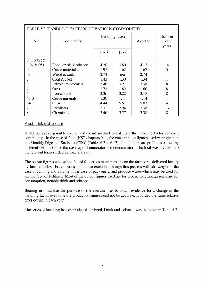
The results of this process, together with the number of years used (where applicable), are shown
in table 5.2; where only a single year has been used this was 1989. As that year marked the
beginning of the current recession, the measured handling factors are higher than would be the
case in more prosperous years. This is because when orders are outstanding and demand is
outstrips supply, there will be less need to place goods at intermediate storage locations in the
distribution chain. A deeper than foreseen fall in demand will cause a greater than average level
of handling, and so the 1989 figures may be above the trend value. We therefore present the
1986 figures for comparison where possible. Given this complication, we do not feel that we
have sufficient data on handling factors to permit us to forecast them in the medium term,
although we have identified some pointers.
The figures show that in general, commodities of low value tend to be handled least often. Other
reasons for handling goods more often, apart from value, are seasonal production or demand
(fertilisers), statutory storage requirements (petroleum products) and a high level of service given
to products for delivery direct to the consumer (foodstuffs).
A handling factor for manufactured goods and miscellaneous articles (NST 9) could not be
estimated accurately. These tend to be made from semi-finished goods, components and sub-
assemblies. Many consumer goods (which are included in NST 9) are manufactured by batch
production methods, and supplied to consumers using complex distribution chains incorporating
a number of inventory holding and break-bulk points. Overall it is unlikely that these categories
of goods will have a handling factor of less than 5 on average.
47
48
TABLE 5.2: HANDLING FACTORS OF VARIOUS COMMODITIES
NST
Commodity
Handling factor
Average
Number
of
years
1989 1986
0+1 (except
04 & 05)
04
05
2
3
4
5
61-3
64
7
8
Food, drink & tobacco
Crude materials
Wood & cork
Coal & coke
Petroleum products
Ores
Iron & steel
Crude minerals
Cement
Fertilisers
Chemicals
4.20
1.95
2.74
1.43
3.46
1.71
3.36
1.30
4.44
2.32
3.46
3.80
1.62
n/a
1.30
3.27
1.82
3.22
1.11
5.51
2.94
3.27
4.13
1.67
2.74
1.34
3.38
1.60
3.18
1.14
5.03
2.38
3.38
14
5
1
11
8
8
8
11
4
13
8
Food, drink and tobacco
It did not prove possible to use a standard method to calculate the handling factor for each
commodity. In the case of food (NST chapters 0+1) the consumption figures used were given in
the Monthly Digest of Statistics (CSO) (Tables 6.2 to 6.13), though there are problems caused by
different definitions for the coverage of numerator and denominator. The total was divided into
the relevant tonnes lifted by road and rail.
The output figures we used excluded fodder, as much remains on the farm, or is delivered locally
by farm vehicles. Food processing is also excluded, though this process will add weight in the
case of canning and volume in the case of packaging, and produce waste which may be used for
animal feed of fertiliser. Most of the output figures used are for production, though some are for
consumption, notably drink and tobacco.
Bearing in mind that the purpose of the exercise was to obtain evidence for a change in the
handling factor over time the production figure need not be accurate, provided the same relative
error occurs in each year.
The series of handling factors produced for Food, Drink and Tobacco was as shown in Table 5.3.

49
TABLE 5.3: HANDLING FACTORS FOR FOOD, DRINK AND TOBACCO
1976-1989
Year Factor Year Factor Year Factor
1976
1977
1978
1979
4/5 year av
5.16
4.33
4.51
4.46
4.12
1980
1981
1982
1983
1984
3.93
4.05
3.66
3.83
3.59
3.81
1985
1986
1987
1988
1989
3.87
3.80
3.95
4.48
4.20
4.06
In these figures there is some evidence that the number of times goods are lifted is declining
slowly.
Other commodities
The Annual Abstract of Statistics provided consumption figures for coal, petroleum, metal
products, fertilisers and chemicals, the totals of which (including exports) were divided into the
tonnes lifted figures obtained from TSGB and CSRGT for the various modes. Apart from some
omissions such as relatively small volumes of speciality chemicals, one problem is that some
coal is consumed by steel works at the point of importation and is not actually lifted by transport
within the UK. Nevertheless, the handling factor established gives an indication of the number
of lifts involved, though it may be conservative.
Some industries do not have statistics on their physical output, the only information being
contained in the Business Monitors in the form of sales values. To convert this into a physical
output figure it was necessary to produce an imputed value per tonne using the Trade Statistics,
which together with imported goods gave the total tonnage delivered. This method was used for
wood and timber, crude materials, ores and minerals.
A complicating factor, we believe, is that handling factors appear to vary over the economic
cycle. There appear to be plausible reasons why this might be the case. For example, falls in
demand that are unforeseen in extent or speed of arrival may leave production ahead of demand
such that the surplus has to be placed temporarily in store. We have analysed available data, but
other than having developed the above feeling, we have been able to identify no clear pattern.
Figure 5.1 presents the series we have derived, together with annual change in GDP.
5.2 LINKING LENGTH OF HAUL AND HANDLING FACTORS
Figures 5.2 and 5.3 show average lengths of haul in kilometres for a range of commodities for
road and rail transport.
When considering changes in the average length of haul, two aspects appear to be most
important: the long-term trend, and cyclical variation. When all commodities are considered

50
together, the long-term trend is towards longer hauls, by 16% over the ten years to 1990. As this
covers an economic cycle this may indicate the long term average. As for cyclical variation the
picture is unclear, as was the case with handling factors (discussed above). Changes in handling
factors are, in any case, likely to be reflected in lengths of haul. Other cyclical effects on length
of haul could arise from recessionary pressure to find new markets, possibly inheriting some
from failed businesses. In the case of firms operating road vehicles on own account, eg. the oil
companies, such vehicles may be used on longer hauls in order to retain maximum utilisation of
the fleet. Production of bulk commodities may also be slower to adjust to the economic
situation, and the output must be moved further if it is to be sold, the reverse occurring in years
of growth.
If it can be shown that the economic cycle induces opposing trends on the length of haul and
handling factors, this would provide a partial explanation for the fact that tonne-kms are more
closely linked with GDP than are tonnes. However, the position is far from clear and further
analysis should be done as better statistics become available. The work on handling factors was
intended to demonstrate that a reduction would indicate a decline in the number of storage
locations within the distribution system. The results are not conclusive. They show that the
economic climate, and changes in demand for a commodity also cause the handling factor to
alter.
To take the particular case of iron and steel, restructuring of the industry had a much more
important effect on average length of haul than a change in demand. However, an additional
factor was the abandonment of wagonload services by BR (except for the Speedlink network).
The length of haul was thus increased by a combination of restructuring within the industry, and
within the distribution system serving it. Length of haul by road increased not only because of
ewer sources of the product, but because of the transfer of some of the longer movements from
rail. The latter may have also resulted in some steel traffic no longer having to be transferred to
road for final delivery.
It is clear that while the trend is for most commodities to have an increasing average length of
haul (except for miscellaneous articles) the progression is not consistent and there is a
relationship with the number of times goods are handled. The restructuring of industry,
particularly the methods used to deliver goods have a greater long term influence on the distance
goods are moved without intermediate transhipment. We expect handling factors to fall over
time, but possibly only very slowly. Lengths of haul can be expected to continue to rise but
probably at a slower rate than hitherto.

54
6.CHANGES IN ROAD DISTRIBUTION PATTERNS AND THE
DEMANDS OF USERS
6.1THE OVERALL POSITION
Most freight traffic within Great Britain is carried by Heavy Goods Vehicles (HGV), soon to be
re-classified as Large Goods Vehicles. By far the most important source of data regarding the
use of HGV's is the published results of the Continuing Survey of Road Goods Transport (DTp
1991a). Unpublished information from this survey has been obtained by private correspondence.
Over the sixteen years from 1974 to 1990 there has been an increase in all the main measures of
freight output. In this period, tonnes lifted increased by 13%, tonne-kilometres by 50%, and the
average length of haul increased by 32%. Taking a ten year cycle, from one recession to another,
1980 to 1990, the increases are 25% for tonnes lifted, 46% for tonnes moved and 16% for the
average length of haul. Comparison of these sets of indicators suggests that by 1980, the largest
generators of traffic may have re-organised their distribution systems to take advantage of the
development of the strategic road network improvements. Since then there has been relatively
little improvement in the strategic network.
Within the overall figures, while tonnes lifted and moved increased in all distance categories, the
figures for over 300 kms are up by 65% in ten years. This implies that the volume of goods
being moved very long distances has seen the most rapid growth, with the average length of haul
for goods moved over 300 kms remaining at around 405 kms. The rapid increase in the longer
distance movements is partly due to manufacturers concentrating production at one, or a small
number of locations.
The introduction of the 38 tonne lorry in 1983 helped this process by reducing freight costs,
particularly for the movement of full loads over long distances. Within the vehicle type
categories, where the change has been measured over the years 1985-90, there has been in
general a slight decline in the use of all types of rigid vehicle, while 32.5 tonne gvw artics have
seen a significant decrease, the traffic now being carried on vehicles with a GVW greater than 33
tonnes. The latter now move 50% of all road freight in terms of tonne kilometres (DTp 1991a),
and have not only absorbed the traffic switched from smaller artics, but also the general increase
in tonnes lifted and moved.
While this gives an assessment of the overall changes, it does not apply evenly among the
various commodity classifications. Changes apparent in CSRGT data have been examined
separately by sector, and an attempt has been made to link these with evidence of changes in the
pattern of industrial structure and the way the commodity is being handled in the distribution
chain.
6.2FOOD, DRINK AND TOBACCO (NST 0 AND NST 1, EXCLUDING 04, 05 AND
09)
The changes in the flows of this important group of commodities probably reflect a different
distribution strategy, plus some change in demand over time. Table 6.1 shows:-

55
Less use of small vehicles.
Fewer short hauls.
Greater use of articulated vehicles.
Large increase in hauls greater than 300 kms.
The total demand remains fairly stable with some influence of the economic cycle in this
category which forms one quarter of all the tonnes moved by road.
TABLE 6.1: CHANGE IN TRANSPORT OF FOODSTUFFS 1985-90
Million Tonnes lifted
% Change
1985 1990
By vehicles
7.5-17t GVW
Articulated vehicles
72
146
55
199
-24
+36
Length of haul
<25 kms
>300 kms
64
15
56
21
-13
+40
Source: DTp (1991a) and the 1986 edition.
Other studies have estimated the handling factor to be approximately five (McKinnon 1989).
However, our calculations (see Chapter 5) produce an average handling factor of 4.13 for food
drink and tobacco, which may be because a greater proportion of basic agricultural products are
included. There was some evidence that the handling factor has been declining over time, which
could in part be the result of a fall in the number of businesses (BSO 1991). Overall food, drink
and tobacco businesses (ie. producers and processors) have declined in number by only 4%
between 1984 and 1989. However, those which generate large volumes of traffic have declined
faster, with grain milling, soft drinks, pet foods and animal feedstuffs falling by 17-19%, while
brewing businesses declined by 30% (Table 6.2). These statistics are comparable with the
changes found in the results of the CSRGT.
6.3 CRUDE MATERIALS (NST 04,09,84)
These include: wool; cotton; man made fibres and other textile materials; hides; rubber; and
paper (including pulp and waste). Tonnes lifted and moved both increased, leaving average haul
length much the same. Within distance categories, traffic increased in bands from 25 to 200 km,
but decreased on shorter and longer hauls.
There was a slight increase in the use of smaller vehicles, and an increase in own account vehicle
use in terms of tonnes moved. This category of goods typically forms part of the production
chain, so we might speculate that the driving force has been a requirement for higher quality
transport services.
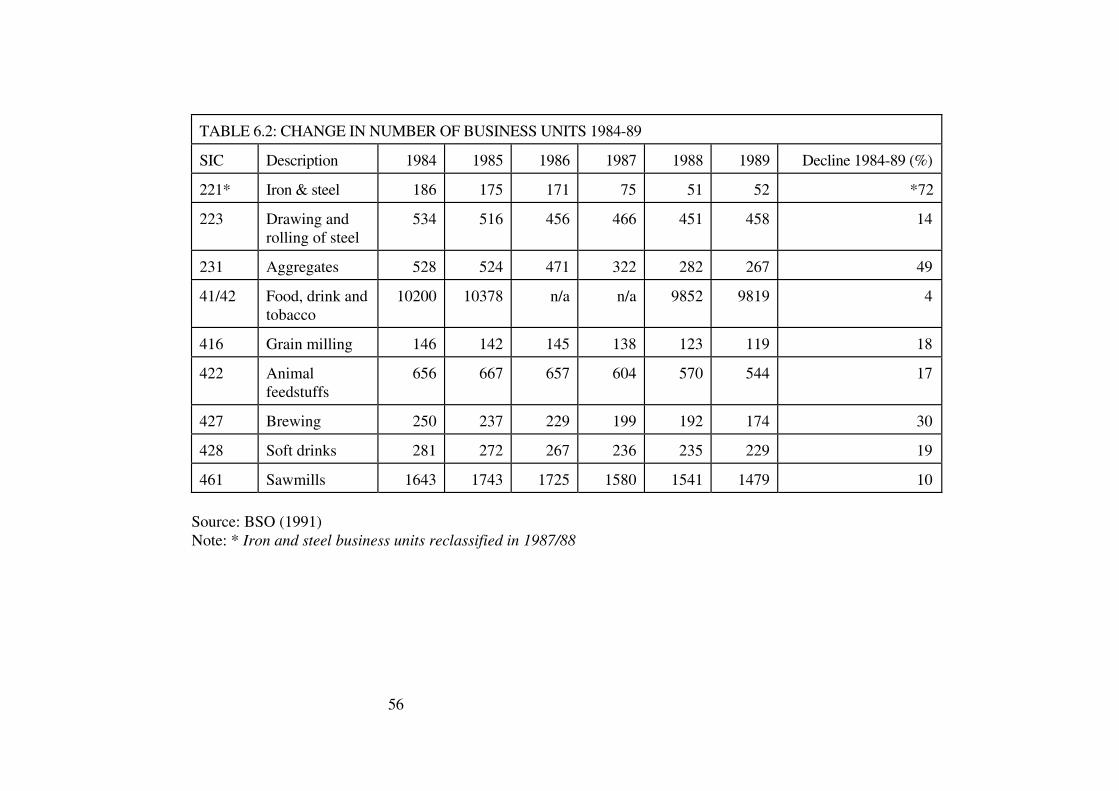
56
TABLE 6.2: CHANGE IN NUMBER OF BUSINESS UNITS 1984-89
SIC Description 1984 1985 1986 1987 1988 1989 Decline 1984-89 (%)
221* Iron & steel 186 175 171 75 51 52 *72
223 Drawing and
rolling of steel
534 516 456 466 451 458 14
231 Aggregates 528 524 471 322 282 267 49
41/42 Food, drink and
tobacco
10200 10378 n/a n/a 9852 9819 4
416 Grain milling 146 142 145 138 123 119 18
422 Animal
feedstuffs
656 667 657 604 570 544 17
427 Brewing 250 237 229 199 192 174 30
428 Soft drinks 281 272 267 236 235 229 19
461 Sawmills 1643 1743 1725 1580 1541 1479 10
Source: BSO (1991)
Note: * Iron and steel business units reclassified in 1987/88

57
6.4 WOOD, TIMBER AND CORK (NST 05)
There is little change in tonnes lifted; the increase in tonnes moved is the result of a greater
proportion of movements greater than 100 kms, especially those of 200-300 kms (+100%).
Greater length of haul may indicate a change in the structure of supply. Wood products are
being imported via fewer ports as a result of new shipping techniques, and are probably
stocked at fewer locations as a result. The BSO statistics show an increase in the number of
businesses making finished wood products (not tabulated), though the number of sawmills
fell by 10% over five years (Table 6.2).
6.5 COAL AND COKE (NST 21-23)
The figures for this commodity are distorted by the miners' strike and the subsequent re-
structuring of the industry. Tonnes lifted is little changed, but haul length has increased
significantly. This may indicate a switch from rail movement at the margin, though road
hauls of coal over 300 km increased by 161% from 1977 to 1989.
Over 90% of the tonnes moved are in vehicles of over 25 tonnes GVW, with a strong
movement from eight wheelers to 38 tonne artics. This may be a general replacement of
elderly rigid vehicles.
6.6 PETROL & PETROLEUM PRODUCTS (NST 31-34, 83)
There has been a significant fall in the tonnes lifted by road vehicles, but this is
counterbalanced by longer hauls, especially those over 300 km. Short hauls have declined,
which may indicate some rationalisation of distribution.
A very high proportion of movements use artics, 44% in those over 33 tonnes GVW. This is
still a commodity carried mainly in own account vehicles, though many petro-chemical
companies have now adopted a policy of using contract distribution.
Fuels, as well as some petroleum products, are trunked by pipeline, rail and sea, as the
volumes on some routes make these modes attractive. Special products, such as liquid
petroleum gas (lpg), tend to be delivered direct by road.
6.7 ORES (NST 41, 45, 46)
Over 12 years demand for ores lifted and moved rose by 40%, haul length remaining the
same at 67 kms. However, within distance categories movements over last 5 years show an
increase in shorter hauls, possibly partly due to side effects of the miners' strike, during
which sympathy action by train crews disrupted supplies of ore to steel works. A switch
from rail at marginal distances may also have occurred.
The miners' strike may also have had an influence on type of vehicle and mode of operation.
Ores are the only commodity where the use of rigid vehicles has increased and artics
decreased. It is also the case that own account operation has expanded at the expense of road
haulage.

58
6.8IRON AND STEEL PRODUCTS (NST 51-56. PIG IRON, CRUDE STEEL
(SHEETS BARS ETC), UNWROUGHT AND NON-FERROUS ALLOYS)
The reduction in tonnes lifted of 18% is probably mainly because of structural change in the
industry, with concentration of production at integrated plants. In terms of tonnes moved, this
was almost counter-balanced by a 16% increase in the length of haul. However, this is confined
to distances greater than 300 km in which category the average length of haul increased from
381 km in 1977 to 423 km in 1989. There was a decline in the traffic in the shorter distance
categories. Of the tonnes moved in 1990, 86% was undertaken by artics, 76% of the total in
vehicles greater than 33 tonnes GVW.
There are a number of subjective judgements required to forecast future patterns of steel traffic.
Will the proposed closure of Ravenscraig go ahead, and if so will it complete the present phase
of restructuring of the industry? Also, there is a problem of plants producing finished items
falling into NST 94, finished products being moved direct from integrated plants instead of semi-
finished steel between plants. The number of iron and steel businesses fell by 70% between
1984 and 1989 (see Table 6.2). For drawing and rolling of steel, the fall was 14%, but the
number of businesses involved in the production of finished metal goods changed little (not
tabulated).
6.9 CRUDE MINERALS (NST 6 EXCLUDING 64 AND 69)
These form 24% of tonnes lifted and 12% of tonnes moved. The fact that there is little change in
average length of haul disguises the fall in traffic travelling between 200-300 km, which is
possibly the result of switching to rail movement to depots in urban areas, and an increase in
road hauls over 300 km, possibly special grade products moved in small volumes. In recent
years, there has been an increase in the volume of aggregates using coastal shipping, probably
reflecting the introduction of supplies from Scottish islands. Over a five year period, there was a
decline in the number of aggregated businesses of 49%.
6.10CEMENTS AND OTHER BUILDING MATERIALS (NST CEMENT & LIME 64.
OTHER BUILDING MATERIALS (BRICK ETC, CONCRETE,GLASS AND
POTTERY) 69, 95)
In addition to an increase in overall demand, there has been a significant increase in movements
greater than 200 km, from 34% to 40% of the tonnes moved. This could be as a result of a
reduction in production locations and/or more choice in the market. However, this is against the
background of cement generally being sold in areas nearer to production points, some longer
distance flows of cement by rail no longer being undertaken, while other flows have switched to
road movement throughout. Cement is another product where there has been a significant
increase in the quantity imported in recent years.
There has also been a significant change in fleet requirements, with a much greater use of artics
operated by hauliers, as opposed to rigids operated on own account.
6.11 FERTILISERS (NST 71, 72)

59
This category forms only 1% of tonnes lifted and moved. Large fluctuations in demand are not
related to economic cycle (1983-84 up 50% for no apparent reason). More important to the
demand for fertilisers are farm prices and food subsidies.
The pattern of transport has changed, with an increase in short haul traffic, medium distance
traffic being reduced. This may be due to contraction in manufacturing locations and an increase
in rail trunk haulage. In the last few years there has been a large increase in the quantity of
fertiliser imported, while a number of UK plants have either reduced output or closed
completely.
6.12 CHEMICALS (NST 81, 82, 89)
There has been a slight increase in demand, but the longer length of haul has increased tonnes
moved significantly. In the 300 km plus distance category, the average haul increased from 370
km in 1977 to 414 km in 1989. This may be due in part to some concentration of production of
commodity chemicals.
There is a marked increase in the use of 7.5 tonne GVW vehicles over short distances. This may
reflect an increase in speciality chemicals being used in the production chain which are delivered
by distributors in small regular batches. There was only a small increase in the use of hauliers.
6.13MACHINERY AND TRANSPORT EQUIPMENT (NST 91-93. VEHICLES,
TRACTORS, ELECTRICAL AND NON-ELECTRICAL MACHINES)
Goods in this category are diverse in nature: capital goods; goods used in the production process;
and some consumer durables. Overall demand seems to be linked to economic cycles, possibly
with some lag.
There has been little change in the average length of haul. Those in the longest distance
categories have seen the greatest increase in volumes. There has been an unusual switch from
artics to rigids, the explanation of which may in part lie in the type of car carriers now being
introduced. Little traffic switched to hauliers.
In recent years, rail has lost a number of flows of assembled vehicles. However, the European
railway operators are hopeful of gaining the movement of considerable numbers of cars between
Europe and the UK following the opening of the Channel Tunnel. This may reduce the road
distance this traffic is moved in the UK, as rail depots are likely to be established near the main
centres of demand, whereas the current method relies mainly on road transport from the port of
landing.
6.14OTHER METAL PRODUCTS, NES (NST 94 STRUCTURAL PARTS ETC)
Tonnes lifted doubled. This is probably due in part to movements of finished products from
integrated plants to point of final demand. The traffic is heavily dependent on the use of the
largest articulated vehicles. Traffic over the longer distances has seen the greatest increase in
volume.

60
6.15MISCELLANEOUS MANUFACTURES (NST 96, 97. LEATHER, TEXTILES
AND CLOTHING, N.E.S.)
Given that there is little increase in goods hauled 25-50 km, and an increase in the other
categories of length of haul, particularly those greater than 200 km, this may indicate structural
change in terms of location of factories and depots. As with groceries, retailers have taken
control of many flows of clothing. The change in favour of large artics would reinforce this
view.
6.16MISCELLANEOUS ARTICLES (NST 98, 99. ARMS, AMMUNITION,
COMMODITIES N.E.S., AND UNKNOWN COMMODITIES)
This category covers 21% of the tonnes lifted and 16% of tonnes moved. There has been a large
increase in the tonnes lifted and moved over all distances, but especially up to 50 km. There has
been little change in the vehicle types used, except for a decline in 17 tonne rigids.
These changes may reflect structural change in industry generally, as well as in distribution.
More goods may be delivered in small vehicles carrying consolidated loads, whether the receiver
is a retailer or car assembly plant. This reflects de-stocking measures which result from just in
time (jit) production methods. The goods are trunked in the largest or most cost effective
vehicle, usually as a one product load, then delivered in small consignments as part of a mixed
load over short and medium distances.
It is thought that a combination of these factors has led to a large variety of commodities now
being classified as miscellaneous in the CSRGT. Previously, the movement would have formed
a one commodity movement but now forms part of a mixed load. The tonnes lifted and moved
of commodities within the production chain and of finished goods are those most likely to be
underestimated as a result of these changes.
6.17 FUTURE TRENDS
The pattern of increasing demand for high quality freight services (not only by road) seems set to
continue. The main pressure for improvement comes from the savings which accrue from
reduced inventories. This has resulted in the widespread introduction of "just in time"
production techniques and the overall management of the supply chain in order to minimise cost.
To achieve the objectives set by industry the distribution system must provide fast and very
reliable services, over great distances. Industry will be prepared to accept higher transport costs
provided the total costs of production and delivery to the customer are minimised for a given
standard of service, or if sufficient added value can be extracted from an improved standard of
service to the customer. This approach also tends to encourage concentration of production and
storage and the trend is likely to continue for many years to come, accompanied by increased
length of haul. However, we do not foresee continued structural change at as high a rate as has
been experienced in the recent past.

61
7. CHANGES IN VEHICLES AND VEHICLE ACTIVITY
7.1 EFFECT OF LEGISLATIVE CHANGES
The introduction of the 38 tonne GVW artic was anticipated by the road transport industry. The
legislation required maximum weight articulated vehicles to have at least five axles instead of
four. Many of the combinations in use in 1983 had been designed so that they could be plated
for more than the then maximum weight in the UK of 32.5 tonnes. This was especially true of
tractor units, which were generally of a design suitable for sale and use throughout Europe; in
fact, many only required re-licensing at the higher weight limit.
The semi-trailers hauled by the units usually needed conversion. However, many had been built
in preceding years with strengthened necks and frames, and had been fitted with tandem axle
bogies which could be easily converted to, or replaced by tri-axle bogies. As a result, a
considerable number of vehicles were operating at 38 tonnes gross within a short time of the
introduction of the new limit, the cost of conversion to the operators being relatively low, and the
incentives being good. In addition, the national fleet was showing signs of being `tired' because
of the recession in the previous years, and as economic activity increased operators decided to
purchase new vehicles. Table 7.1 shows the changes in the fleet composition.
Using estimates given in `The Allocation of Road Track Costs' (DTp, various years) between
1983/84 and 1985/86 the change from four axle 32.5 tonne artics resulted in a decline in their
numbers of 32,200, (40%) either being converted to or replaced by the 24,500 38 tonners
introduced (DTp 1983). It has been estimated that just over half of these were new vehicles, the
rest being re-licensed (Johnson and Wilding, 1986).
Initially, the flows of traffic where they would generate the maximum revenue were the longer
hauls. As a result, the average length of haul and the payload were at their highest for the 38
tonne GVW category in the years immediately after their introduction. The payload of vehicles
with a GVW greater than 33 tonnes was at its highest in 1985, two years after their introduction.
Over the period 1985 to 1990 the payload of articulated vehicles of less than 33 tonnes was
reduced by 21% as they now tended to specialise in the carriage of goods which were
constrained by volume rather than weight, whereas for those over 33 tonnes the payload fell by
9% as they expanded their market penetration into the movement of less dense commodities. It
should be noted that the general trend was for most types of vehicle to have lower average
payloads over this period (Table 7.2).
Vehicles of over 33 tonnes GVW now have a significant role in the movement of most
commodities. Exceptions, such as aggregates and minerals, are generally moved shorter
distances so that the lower unit cost advantages of the larger vehicle are not so important.
Other commodities such as petroleum products, cement and building materials require more
specialised vehicles. The conversion of the more specialised fleets has taken longer, but the
current recession has probably led to the early disposal of some of the older vehicles with lower
capacity, thus increasing the penetration of the largest articulated vehicles in the market which

62
remains.
TABLE 7.1: CHANGES IN FLEET COMPOSITION (000's)
GVW 83/84 85/86 87/88 89/90 91/92
Rigids
3.5-7.5 - 151.1
40%
154.1
41%
162.9
39%
165.8
40%
12-13 24.0 22.7
6%
20.1
5%
17.8
4%
15.7
4%
15-17 74.2 80.3
22%
82.1
21%
88.6
21%
86.7
21%
23-25 24.7 27.1
7%
25.5
7%
27.0
7%
26.4
7%
29-31 14.9 16.7
5%
18.1
5%
21.9
5%
21.1
5%
Artics
26-28 2.6 3.9
1%
5.5
1%
7.5
2%
8.2
2%
31-32.5 81.1 48.9
13%
37.3
10%
33.8
8%
24.7
6%
36-38
(2+3 axle)
0.7
19.4
5%
24.0
6%
33.9
8%
36.8
9%
36-38
(3+2 axle)
4.2
1%
9.8
3%
14.9
4%
17.7
4%
36-38
(3+3 axle)
0.9
0%
3.3
1%
6.2
2%
9.8
2%
Source: DTp (1991c) and previous editions.

63
TABLE 7.2: AVERAGE PAYLOAD WHEN LOADED AND LOADED KILOMETRES
PER VEHICLE 1985/1990
1985 1990 % Changes
Tonne
'000
km
Loaded
'000
km
Payload
tonnes
Tonne
'000
km
Loaded
'000
km
Payload
tonnes
Loaded
'000
km
Payload
tonnes
Rigids
<7.5
tonnes
21 14 1.50 28 19 1.47 +36 -2
7.5-17
tonnes
95 23 4.13 115 28 4.11 +22 0
17-25
tonnes
263 23 11.44 248 24 10.32 +4 -10
>25
tonnes
522 30 17.40 533 32 16.66 +7 -4
Artics
<33
tonnes
549 44 12.48 492 50 9.84 +14 -21
>33
tonnes
1115 59 18.90 1079 63 17.13 +7 -9
All
HGVs
225 26 8.81 279 32 8.72 +23 -1
Source: Derived from DTp (1991a) and previous editions.
Commodities near the end of the production chain have a greater tendency to be volume rather
than weight constrained. They do not benefit to such an extent from carriage by heavier lorries,
but would receive greater benefits if the volume carried could be increased.
The two axle rigid lorry of between 7.5 and 17 tonnes GVW is the vehicle primarily used for
local distribution, but also increasingly for smaller consignments of time sensitive goods within
the production chain. Nevertheless, the tonnes lifted in a wide range of commodities
demonstrates the classic distribution pattern of trunk movements being dominated by the use of
the largest possible vehicles, two axle rigid vehicles being used for final delivery over relatively
short distances. Examples of commodities which use this pattern of distribution are beverages,
food, and most consumer goods categories.
Other legislation has led to the introduction of longer artics, the limit being recently increased
from 15.5 metres to 16.5 metres. Though statistics are not readily available, it is apparent that

64
the introduction of longer articulated vehicles will be a slower process when compared to the
reaction to the heavier vehicle. This may in part be due to there being a smaller range of
commodities which require vehicles with greater volume. Alternatively such commodities can
be carried in 18.5 metre draw-bar outfits. However, the main reason for the slow introduction of
longer articulated vehicles is that the legislative requirements demand the trailer bogie to be
positioned differently. This is in order to conform to new Construction and Use Regulations
regarding the turning circles of longer outfits. This means that little current equipment can be
converted. Operators will tend to introduce the longer trailers only when existing equipment is
life expired, or to meet new traffic demands. Nevertheless, the longer trailers are preferred by
the supermarket chains; ASDA obtained a derogation in order to purchase them before the
regulations came into force.
7.2 FORTHCOMING LEGISLATIVE CHANGES
The changes in lorry weights over the coming decade are largely designed to harmonise the
position in the UK with EC Directives. The anticipated changes are shown in Table 7.3.
TABLE 7.3: CHANGES TO MAXIMUM VEHICLE WEIGHTS
Vehicle Current 1/1/93 1/1/99
Rigid
2 axle
3 axle
4 axle
17.00
24.39
30.49
17.00
25/26*
30.00
18.00
25/26*
32.00
Articulated
3 axle
4 axle
5+ axle
4 axle drawbar
24.39
32.52
38.00
32.52
24.39
35.00
38.00
35.00
24.39
36/38*
40/44*
36.00
Source: Civic Trust (1990).
Note: * Differential rules explained in text.
In the case of the heaviest articulated lorries, from 1999 the normal limit will be 40 tonnes
GVW, but under current EC plans they will be allowed to operate at 44 tonnes when on a
journey to or from an inter-modal depot carrying a unit for movement by rail. The three axle
rigid vehicles will only be allowed to operate at 26 tonnes GVW if they are fitted with air
suspension as this has been found to impose less damage to road infrastructure for a given axle
weight than traditional suspension designs.
The speed at which operators take advantage of the increased weights depends on a number of
factors. The most important of these is the time they have from the issue of the detailed
Construction and Use Regulations to the introduction of those regulations. If such regulations
demand only minor modifications, these can be undertaken in a short time. Where existing
65
vehicles cannot be modified, operators will have to await the design and production of new
equipment to replace the existing fleet. This process also tends to cause disruption in the
automotive industry as operators delay renewal of their fleets until equipment to meet the new
legislation is available, then order such vehicles in quantities greater than normal.
Many operators tend to purchase vehicles which are designed to operate at weights higher than
the current legal limit allows. By doing so they gain benefits in terms of the reliability and
durability of the equipment. In assessing the changes to the gross weights proposed in Table 7.3,
as large numbers of operators currently use articulated tractors which can be plated at 40 tonnes
or above, many of them merely require to be re-licensed at the new weight. This presupposes
that the current axle spacing will remain, and that air suspension is not required. However, even
if air suspension is required, many operators are now using equipment so fitted, though this
applies mainly to tri-axle semi-trailers, less so to the tractor unit.
Changes to the weights of rigids and four axle articulated vehicles are likely to demand changes
to axle spacing requirements and the use of air suspension. This indicates that apart from
equipment which can be converted, the application of the new weight limits will tend to await
the introduction of replacement vehicles. It is likely to be several years before vehicles plated at
the higher weights form a significant proportion of these categories.
Obviously the primary consideration in the choice of vehicle is the operating cost per net tonne
mile, and the suitability of a vehicle design and specification for the type of work being
undertaken by the operator. In general, the larger the vehicle the less the cost per payload tonne
kilometre. As the cost of operating, for example, a 32.5 tonne GVW lorry is only slightly higher
than that of 28 tonnes, and the cost of turning down an occasional payload greater than the
smaller lorry can carry is high, most operators purchase vehicles which are the maximum for a
given axle class. Exceptions are where a lorry of lower gross weight is more suitable for a
specific regular task.
In summary, we can say that the take-up of the relaxation of the weight limits will not be
determined by the amount of traffic suitable for such lorries, although they will be used on that
traffic first. Rather, because of the minimal extra cost of running lorries plated at the higher
weight, it will be economically advantageous to introduce such lorries as circumstances permit
even if the extra weight capacity is only rarely needed.
7.3 EFFECT OF THE TRANSPORT ENVIRONMENT
There is no doubt that operators will take advantage of new regulations which allow them to
introduce vehicles which will make greater profits, or to operate their fleets more efficiently.
The long term trend is clear from Figure 7.1. However, the transport environment in which they
operate, particularly the nature of the traffic they move and the customers they serve may limit
the extent and speed of application of legislation which changes vehicle technology or operating
methods. An indication is the penetration of each vehicle weight category in each commodity
class (see Table 7.4).
The percentage of kilometres run empty has changed little over the period, remaining stubbornly
about 30% of the total for most categories of vehicle. Exceptions to this are the large rigid

66
vehicles which appear to have little opportunity to obtain return loads, over 40% of their total
kilometres being run empty. This is probably because large rigids tend to be made up of
specialised vehicles such as tippers for the movement of bulk solids, tankers for the delivery of
petroleum products and on-board crane lorries for moving bricks etc. The specialised nature of
these vehicles restricts their availability for back loads, and the products moved by such vehicles
have a relatively short average length of haul, further reducing their ability to collect a load on
their way back to the point of origin. The average length of haul in the largest rigids in the case
of sand, gravel and clay is only 28 kilometres.
Another problem when considering vehicles for use in quarries and such like is the rough
surfaces encountered, where adhesion can be improved by the use of double drive bogies fitted
to many tippers. When discharging at many sites, the ground is not level and large articulated
tipping vehicles tend to be less stable than rigids and are more prone to topple over.
It is in the carriage of commodities moving short distances, where specialised vehicles are
required, that 38 tonne artics have made least penetration. If the vehicle is very expensive to
replace, the operator may wait until the current fleet is life expired before investing in
replacements. The fact that many such vehicles are mainly on short hauls tends to decrease the
benefit of larger capacity because there is a tendency for the vehicle to spend a greater proportion
of its time at terminal sites; the benefits of larger capacity occur when the vehicle is moving
goods, not loading and unloading.
The market penetration of 38 tonne vehicles has proved to be considerable, over a wide range of
commodities. To enable them to carry light goods cost effectively step frame trailers have been
purchased in considerable quantities. These allow a greater internal volume, or in some cases
two decks, reducing the unit cost per cubic metre of goods carried (see Fig.7.2).
One problem encountered in the movement of some goods, bulk liquids and containers for
instance, was that the weight of the front of the semi-trailer tended to overload the drive axles of
2+3 axle combinations. Operators generally overcame this problem by purchasing tri-axle
tractor units. Using such units also allowed some specialised semi-trailers with tandem bogies
that could not be converted to tri-axle trailers.
7.4 VEHICLE STOCK AND REPLACEMENT
The overall level of economic activity has a strong influence over the age of the national vehicle
fleet, and the replacement and scrappage policies of operators. Table 7.5 shows clearly how
operators tend to purchase new lorries in years when economic expansion is at a high level, and
if the traffic demand is sufficient they tend to keep older vehicles in service for longer than
would otherwise be the case.

77
TABLE 7.5: PERCENTAGE OF ARTICULATED STOCK BY YEAR
1984 1985 1986 1987 1988 1989 1990
> 8 years old
5.2
5.5
6.3
8.9
11.0
10.4
8.8
1976
1977
1978
1979
1980
1981
1982
1983
1984
1985
1986
1987
1988
1989
1990
3.8
6.9
11.4
15.3
11.5
9.3
10.7
12.0
13.8
4.8
8.7
12.8
10.1
8.6
10.4
11.7
13.2
14.2
6.2
9.9
8.3
7.5
9.6
11.0
12.5
13.7
14.6
7.9
6.7
6.3
8.5
10.1
11.7
13.0
12.9
14.2
5.0
5.0
7.1
8.7
10.5
11.8
11.9
13.4
15.9
3.5
5.5
7.0
9.1
10.6
10.7
12.3
15.1
15.5
4.4
5.6
7.9
9.9
10.3
12.0
15.2
15.8
10.4
Year on
year change
in GDP
2.8%
3.6%
3.3%
4.6%
4.9%
2.5%
0.2%
Source: Derived from DTp (1991e)
As an economic recession reduces demand for transport services, the number of new vehicles
purchased declines rapidly, both as a percentage of the fleet and in actual numbers, as occurred
in 1990. However, some larger operators de-license a proportion of their fleet in a recession, and
bring such vehicles out of storage either to meet traffic demands or to replace life-expired
vehicles. Such vehicles do not appear on the list of vehicles licensed while they are stored. Note
that in 1990, vehicles first registered in 1989 formed a higher proportion of the fleet than these
vehicles did in 1989.
Where legislation has changed, a recession may result in the early withdrawal from service of
vehicles of outdated specification. Thus the current recession has seen a further decline in the
number of 32.5 tonne GVW articulated vehicles. Operators prefer to use newer 38 tonners,
which also offer the flexibility to carry larger payloads as and when these occur.
Rigid vehicles follow a different replacement cycle to articulated lorries. The percentage of
rigid vehicles over nine years old in 1990 was 17.8%, while that of one year old vehicles was
9.6%. In overall terms rigid vehicles are kept in service longer than artics. Given that rigid
lorries cover significantly fewer kilometres per annum than articulated vehicles, this may

78
indicate that operators base life expectancy of their fleet partly on the total mileage run, and not
only on age.
The type of vehicle body has also changed during the last decade, mainly because of the
introduction of curtain-sided vehicles (particularly semi-trailers) replacing flats (DTp 1991d).
Unfortunately vehicles with this type of body are classified as 'other' in Government statistics
and the extent of their penetration in the total fleet is not known. However, in recent years there
has been a significant fall in the proportion of vehicles fitted with flat or low-sided bodies. There
is also a slight increase in the numbers of vehicles with specialist bodies, which may limit the
opportunities to collect return loads. Vehicles with a type of body no longer suited to current
traffic demand are more likely to be withdrawn from service before they are life expired.
7.5 PRESSURE FOR CHANGE IN VEHICLE USAGE
Customer demand is the driving force behind most changes in the transport industry. Since the
Transport Act 1968, road transport in the UK has been able to act without restrictions on its
commercial decisions. As a result, each operator has attempted to serve a group of customers as
best it can, by offering a service often tailored to their individual requirements in terms of cost
and quality of service. Road transport is also generally used as the benchmark for the alternative
modes.
In providing a tailored service, the road transport industry uses a variety of vehicles of various
weight and size combinations. The vehicle chosen for a given operation will, in the long term at
least, be one which provides a satisfactory service at minimum cost. Legislation seeks to prevent
the use of unsuitable vehicles. Where changes in legislation are being considered, the benefit to
both the industry and the economy will be slower to take effect if new vehicles are required, as
opposed to the conversion of part of the existing fleet.
The taxation of goods vehicles is a significant cost borne by their operators. It is possible that, in
future, taxation could be used to a greater extent than hitherto in order to influence the choice of
type of HGV used, with respect to the vehicles effect in terms of damage to the road. Legislation
on the total number of vehicles, or haulage tariffs, would result in a less efficient road transport
industry.
The combination of new legislation with changes in the structure of the distribution industry, and
the sizes and types of vehicles used, has resulted in increased vehicle productivity.
Consequently, the rate of increase in road freight traffic is lower than that of goods produced.
Assessment of this relationship is important for traffic forecasting purposes. While most
forecasts deal with projection of tonne kilometres, the relationship with vehicle kilometres will
change over time. In part this is the result of structural changes in industrial location, population
and many other factors. However, changes in transport legislation, especially those affecting
vehicle weights and dimension must be taken into account when estimates of vehicle kilometres
are derived from estimates of tonne kilometres. As we have shown, the penetration of vehicles
of various types differs between commodities.
Given that the effect of previous increases in maximum vehicle weight have worked their way
79
through the system, we would now expect vehicle kilometres to rise almost as first as tonne
kilometres until the next major change in vehicle weights in 1999. However, a complete
analysis would relate this to forecasts of future tonnes moved by commodity, as changes in the
commodity structure and length of land may still produce shifts in mean vehicle loads.
8. THE USE OF SMALL GOODS VEHICLES
8.1 COMMENTARY
Small Goods Vehicles (SGV) are those of less than 3.5 tonnes GVW, previously known as light
goods vehicles. Although detailed annual surveys are carried out for vehicles over 3.5 tonnes to
determine how operators use them and what they carry, little is published concerning the
purposes for which owners use these smaller vehicles. Estimates of the distances covered by
these vehicles can be derived from traffic count data. Estimates of the total numbers for some
weight categories are given in the annual published data on the allocation of road track costs and
in TSGB. However, from 1984 light vans have been taxed as private, light goods (PLG), and
from 1990 this included goods vehicles of less than 3.5 tonnes GVW. This makes estimating the
change in their numbers much more difficult, though future use of DVLC records will improve
the situation.
For vehicles of less than 3.5 tonnes GVW, the average kilometres covered per vehicle per annum
increased only 6% during the 1980's. This figure rises to 19% over the last seven years (1984-
1990), after an earlier fall. The number of new small goods vehicles first registered in 1988 was
117,662, an increase of 15% on the previous year (SMMT, 1990). However, the total number of
small goods vehicles licensed increased by 47% over the 1980s, once again most of the increase
being in the late eighties (DTp 1991b).
The main uses of vehicles in this category are:
(a)The carriage of goods.
(b)Use in connection with a trade or business.
(c)Use by maintenance personnel, such as the telephone engineer.
(d)Personal transport for individuals, travellers and representatives, such as meter reading
personnel of utilities.
(e)Vehicles registered as PLG which are preserved coaches or lorries.
The fact that car tax (a remnant of purchase tax) does not apply to small vans still encourages a
small minority of motorists to buy them purely for personal transport. Nevertheless, the vast
majority of vehicles, and particularly vehicle kilometres, are connected with commercial
activities.
The change in numbers and operating characteristics is in part due to the demand for high quality
distribution services in some sectors. This applies to the expansion of the parcels sector, offering
very short transit times for small consignments. Many firms also have developed distribution
systems which can deliver small consignments on short order lead times to conform to the
demand for "just-in-time" manufacturing patterns, and to win additional business.
The expansion of operators offering direct home deliveries in competition with the Post Office is

80
another factor. Initially this type of operation was largely confined to mail order catalogue
deliveries. National parcels carriers, such as Federal Express, now offer such services; in the
case of home deliveries a vehicle from each carrier has to cover each area each day, partially
duplicating vehicle kilometres.
During the 1980's a large number of small businesses were started. Many of these required a
small van as a means of supplying both the business and its customers. At the same time, firms
found that because labour costs were now high, staff who were required to travel as part of their
duties could be made more productive if they became mobile. The cheapest method for
industries such as utilities was to provide staff with small vans. Also, because of increased
labour costs, many firms contracted out maintenance work rather than employ their own staff.
The increase in the number of such service companies helped fuel the rise in the demand for light
vans and pickups.
TABLE 8.1: LIGHT VAN TRAFFIC BY ROAD CATEGORY 1980-1990 (%)
Year 1980 81 82 83 84 85 86 87 88 89 90 10 year
increase
Motorway 8 8 9 9 10 11 13 13 14 14 14 161
Major roads
Built-up
24
23
23
22
22
21
22
21
21
20
19
20
Major roads
Non built-up
25
24
25
27
27
27
27
28
27
28
27
70
Minor roads
42
45
44
41
41
41
40
38
39
39
40
49
Yearly
increase
All roads
1
-1
0
6
3
5
9
11
10
2
56
Source: Derived from DTp. (1991d)
Some support for this analysis can be derived from published data in the form of the percentage
of total kilometres covered by light vans on various categories of road (Table 8.1). In overall
terms, light vans have increased their total vehicle kilometres by 56% during the 1980's. This
compares with about 30% for HGV's.
It is in the use of different categories of road that the greatest changes have occurred. The
percentage of SGV kilometres on motorways has risen from 8% to 14%, a rise for the total fleet
of 161%. This is most likely the result of a combination of time sensitive deliveries to
manufacturers of small consignments of goods, and parcels delivery firms locating depots at
strategic intersections of the road network. This allows a minimum number of depots to serve a
large geographic area, though the small vehicles then cover greater stem mileages on high
quality roads in order to reach their delivery round.

81
The percentage of kilometres on non-built-up major roads has also increased, but only slightly,
though in terms of total vehicle kilometres the rise is 70%. The reverse is the case on minor
roads in percentage share terms, though vehicle kilometres are still up 49%, whereas on built-up
major roads they are up only 20%. In terms of the percentage share this category of road is used
this represents a 5% fall over a decade.
Thus, light vans are using roads more, but high quality roads a great deal more. Survey work
over a period of years is the only accurate method for determining the changes in the use of roads
by such vehicles, and the type of activity on which they are engaged. However, a combination
of a large increase in the quantities of time sensitive small consignments and parcels carriers
serving larger areas from a reduced number of locations appears to be the most likely
explanation for much of the increase.
8.2ECONOMETRIC MODELLING OF THE USE OF SMALL GOODS VEHICLES
This section looks at the problems which occur in forecasting the use of small goods vehicles.
There are problems of definition, which has changed over the years, and data acquisition
problems. The CSRGT does not cover vehicles under 3.5 tonnes gross laden weight, and so a
detailed analysis similar to that of chapter 4 is not possible. However, we can use the differences
in estimates of tonnes lifted provided by CSRGT and TSGB to obtain a figure for tonnes lifted
by small goods vehicles, that figure being the difference between the two. Another problem is
the stock of small vehicles. The figure used is the "other vehicles" category from "private and
light goods" in TSGB; this is vehicles not exceeding 1525 kg unladen weight. Although we
cannot obtain a reliable figure for tonne-kms moved by small goods vehicles, TSGB provides a
series for vehicle kms by light goods vehicles. We can thus model:
Tonnes lifted or Gross Domestic Product or
⎡ vehicle kms or ⎤ = f ⎡ time or ⎤ . ⎣ No of vehicles ⎦ ⎣ Sectoral Output ⎦
Another option would have been to use the output of service industries. However, this is so
closely correlated with GDP (and a regression on the output indices produces a coefficient of
approximately one) that there seems no advantage in repeating the exercise.
Vehicle stock
Over the years 1980-1989, the best time trend model was exponential in form (t statistics in
brackets):
ln(SGV) = -73.5 + 0.0408 YEAR
(18.8) (20.7)
R2 = 0.9816 ȡ = 0.09
This model predicts 2.75 million SGVs in 1995 with 95% confidence limits 2.58 million and
2.94 million (1990 figure is 2.25 million) and 3.38 million (3.11 million to 3.67 million) by
2000.

82
The log-linear GDP model, reported below, gave an elasticity of vehicle stock with respect to
GDP of 1.27 (s.e.=0.067). This model suffered from autocorrelation.
ln(SGV) = 1.64 + 1.27 ln (GDP)
(5.3) (19.0)
R2 = 0.9782 ȡ = 0.27
We also investigated a model which expressed the number of SGV's as a function of time and
deviations from the trend in GDP (DEVGDP). This gave an elasticity of vehicle stock with
respect to deviations from the trend of GDP of 0.58.
ln(SGV) = -6.31 + 0.036 YEAR + 0.583 DEVGDP
(11.0) (12.4) (2.20)
R2 = 0.9891 ȡ = 0.20 F = 318.7
This does not give improved predictions.
Tonnes lifted
Here, the models calibrated related the tonnes lifted by SGVs to GDP and (separately) the output
of NST sectors 98 and 99 (miscellaneous articles) (denoted I9899). This sector was chosen as
being one with a large use of SGV's. Linear and double-log models for both independent
variables all had R2 in excess of 0.95. It is difficult assess the autocorrelation since there are so
few (10) observations; but the GDP linear model appears, from inspection, to suffer. The
double-log model gave an elasticity of tonnes lifted by SGVs (SGVTON) with respect to GDP of
2.1:
ln(SGVTON) = -5.44 + 2.13 ln(GDP)
(9.9) (17.8)
R2 = 0.9755 ȡ = -0.08
Using deviations from GDP, the elasticity was 3.15.
ln(SGVTON) = -69.9 + 0.04 YEAR + 3.15 DEVGDP
(6.02) (6.4) (5.86)
R2 = 0.9840 ȡ = -0.375 F = 215.6
For I9899, the linear model was slightly better, giving an elasticity in 1989 of 2.26:
SGVTON = -137.8 + 2.15 I9899

83
(10.2) (16.2)
R2 = 0.9703 ȡ = -0.1
A model using deviations from I9899's trend gave an elasticity of tonnes lifted with respect to
deviations of 1.86.
ln(SGVTON) = -71.2 + 0.04 YEAR + 1.86 DEVI9899
(4.7) (5.0) (4.33)
R2 = 0.9744 ȡ = -0.225 F = 133.1
Vehicle kilometres
These models all suffered from autocorrelation, and there was not much between them in terms
of fit.
ln(SGVKMS) = -3.5 + 1.47 ln(GDP)
(3.9) (7.5)
R2 = 0.8766 ȡ = 0.51
ln(SGVKMS) = -34.7 + 0.02 YEAR + 2.83 DEVGDP
(1.7) (1.85) (2.96)
R2 + 0.9051 ȡ = 0.31 F = 33.4
ln(SGVKMS) = -5.6 + 1.93 ln(I9899)
(6.9) (11.0)
R2 = 0.9376 ȡ = 0.3
ln(SGVKMS) = -25.8 + 0.01 YEAR + 2.0 DEVI9899
(1.5) (1.7) (4.1)
R2 = 0.9379 ȡ = 0.27 F = 52.8
All these models illustrate the rapidly increasing use of SGV's over the 1980s. They cannot
answer the question of whether these trends will continue, although with the continued growth in
the service industries, and in just-in-time deliveries, it seems likely that they will.
8.3 CONCLUSION
The 1980s saw a growth in the use of SGVs, as measured by vehicle kilometres, of some 56%,
or almost twice the growth in use of HGVs. In that time, the number of SGVs rose by 47%,
from 1.53 million to 2.25 million. A time trend model predicts that the number will rise further

84
to 3.38 million by the year 2000. Tonnes lifted by SGVs was much more sensitive to GDP than
tonnes lifted by HGVs, the elasticities being about 2 and 1 respectively. Likewise, the elasticity
of tonnes lifted with respect to output of miscellaneous articles is greater for SGVs than for
HGVs. If this sector continues to grow in importance relative to other sectors, we will see a
greater than anticipated increase in total freight movement by road. However, an exercise such
as the Continuing Survey applied to SGVs over a number of years is the only way to establish in
more detail the changes in the use of such vehicles. At present, the available data sources do not
permit such an analysis.
9. FREIGHT MODE CHOICE
9.1 INTRODUCTION
Since the Second World War road transport has become increasingly dominant in the movement
of freight in the UK. In general, traffic which has switched modes has transferred from rail to
road, though coastal shipping and inland waterways have also lost traffic, some of it going to rail.
Pipeline traffic has been slowly increasing, though this mode is very specialised and tends to
compete with rail on routes where there is a very large volume of one commodity from one, or a
group of, manufacturers. For example, a consortium of petrochemical companies operates the
ethylene grid, a pipeline which runs from Mossmorren in Scotland, via Grangemouth and
Teesside, to consumers in Cheshire.
What is not appreciated by many people is that the economy of the country has not only
expanded, but the expansion has taken place mainly in the demand for the sort of goods and over
distances, for which road transport currently has a comparative advantage. Rail and water have,
in fact, retained significant quantities of their traditional bulk traffics such as coal and steel.
They have also gained new flows of certain commodities such as petroleum products and
aggregates.
Nevertheless, the general pattern has been one of an overall decline in rail freight traffic. In
many cases it has not been the result of a switch of mode, but of the decline of the country's basic
industries, on which rail depended for much of its traffic. The rate of decline of tonnes moved
by rail, which in overall terms was about 3% per annum until 1979, has accelerated due to major
restructuring undertaken by manufacturing industry during the last decade (Fowkes et al 1987).
9.2 DEVELOPMENTS IN DISTRIBUTION SYSTEMS
The pace of change within the transport industry shows considerable variation between different
market sectors. In the case of coal and iron ore, the concentration of production and the
construction of large coal fired generating stations since the war has allowed the introduction of
high capacity handling equipment and large units of carriage, whether they are ships, push-tow
barges, or block trains. Because volumes moved of such commodities can be very high, the unit
costs of the use of both the handling equipment and the rail infrastructure can be kept low.

86
It is for this reason that rail, usually considered to have a competitive advantage on long hauls,
can gain large quantities of traffic travelling just a few miles. Many movements of power station
coal take place over distances of no more than 40 kilometres. Thus volume is an important
factor when comparing the costs of different modes. Unfortunately, it is the heavy industries
which have suffered the greatest decline since 1979, restricting the opportunity for BR to exploit
the new developments in the rail movement of such traffic. Nevertheless, they have successfully
applied the principle to marketing their services to aggregates producers, and for the movement
of waste to reclamation sites.
There is a considerable contrast in the situation in sectors such as steel, consumer goods and
groceries. Such sectors have been much more buoyant and the change in their distribution
techniques more rapid. The major driving force has been a change in business outlook.
Companies, rather than search for the cheapest method of transport, aim to minimise the overall
cost of production and supply of goods. An increased cost in one distribution activity may be
traded off against a saving in another activity so as to provide an overall cost reduction.
Improved methods of handling have evolved steadily, and together with the introduction of
information technology, have assisted this process by providing greater scope for cost savings.
Thus, the activity of transporting consumer goods must be seen as part of the total supply chain
activity. This requires, in general, high levels of service to be offered not only for the finished
product, but also in sourcing raw materials and components, in order to minimise inventories
throughout the production chain. Techniques such as "just-in-time" (jit) and 'materials
requirement planning' (mrp) have been introduced to achieve cost reductions, but these tend to
demand the delivery of small consignments at frequent intervals. The distribution industry has
been forced to achieve two seemingly conflicting objectives simultaneously: to reduce costs; and
to improve service levels.
Decisions on the method of distributing goods, including choice of mode, are not generally made
on the basis of an individual consignment. Instead they are decided at the strategic planning
stage. Such plans will establish the service level required and whether the manufacturer or a
transport operator will provide the equipment. Modal choice is unlikely to change until there is a
periodic review of the distribution system as a whole, which could be undertaken for a variety of
reasons including changes in the relative costs of the methods used and the modes used,
obsolescence of essential equipment, or the development of new technology. This is not to say
that all firms will deliberately forsake the option of keeping a range of modes available for use,
for example the distribution of petroleum products from refineries which uses several modes.
One method by which many firms have managed to achieve improved service at little additional
cost is the establishment of regional depots or distribution centres (rdc's). It is possible to
provide next day deliveries to customers from only a small number of rdc's. If a 48 hour lead
time is required, excluding the time for order processing and picking, then only one depot is
required to serve the mainland of Great Britain. If the lead time falls to 24 hours then a
minimum of two rdc's are necessary. Most firms have more than two, either to improve the
service, or because the volume of goods to be handled exceeds that level above which no further
worthwhile economies of scale are available. The extent of such economies depends on the scale
of manual picking operations in the warehouse (Weber 1990). Where the goods to be picked are
in standardised units (such as full pallets), automation of a minimal number of warehouses can

87
reduce costs more than the additional transport costs incurred if fewer depots are used.
However, few firms are likely to have the volumes of standardised packages required to justify
fully automated warehouse systems. With non-automated systems it is possible even that
diseconomies of scale may be important.
In order to minimise the number of depots they must be sited with care so as to exploit maximum
potential from the strategic road system. Such depots are, in many cases, served by overnight
trunk delivery road vehicles from factories or suppliers. This method of distribution promotes
better utilisation of vehicles, warehouse staff and equipment while minimising stock in the
system. Manufacturers can only justify establishment of their own networks if they have a
considerable demand for distribution services.
Firms have further reduced the stock held in the distribution system by the use of stockless, or
satellite, depots. These are effectively signing on points for drivers served by pre-loaded
vehicles despatched from a main depot, again usually overnight.
Dedicated distribution systems such as these can be highly capital intensive. To enable smaller
companies to benefit from these distribution techniques, specialist hauliers and distribution
contractors offer such services on a common user basis. Under such a scheme, several
manufacturers and suppliers would share the facilities offered. The availability of such schemes
has resulted in some firms' abandonment of their own account transport operations.
9.3 DETERMINANTS OF FREIGHT MODE CHOICE
9.3.1 Introduction
Forecasting mode choice for freight transport is generally more difficult than for passenger
traffic. There is relatively little data available to calibrate models, and the information
requirements are considerable. Whereas forecasting mode choice for a passenger from A to B
can be reduced in its simplest form to considering the effects of price and quality, freight has the
additional complication of physical and technological constraints, since it comes in various
shapes, sizes and physical states. There is also the question of the requirements of the consignee.
We might therefore depict a model of freight mode choice as:
Probability Characteristics of consignment, characteristics of consignor
⎡ of choosing ⎤ = ⎡ ⎤ ⎣ mode x ⎦ ⎣ Characteristics of consignee, characteristics of feasible modes
⎦
In the short term, with fixed locations of consumers, suppliers and depots, and with a given
transport infrastructure, the characteristics of feasible modes can be expressed in terms of the
cost of moving the load, the transit time, the reliability of the service and the number of (possibly
inter-modal) transhipments. The relative weights attached to these characteristics can be
expected to vary according to the nature of the product (physical state, value per tonne, volume
of flow), the extant distribution network and inventory levels. The problem with a short term
analysis is that the important choices are usually decided at a strategic level rather than at
individual consignment level, so the mode choice decision will be a comparatively rare event and

thus, in the short run, an unrealistic situation. Nevertheless, the potential for trade-offs between
different service attributes must ultimately exist. In the longer term, changing patterns of
demand, supply and distribution networks will impact on mode choice and on the choice set of
feasible modes. Thus in the long run, the overall logistics of companies need to be predicted, as
well as changes in industrial structure. An indicator of the way things are changing is the
increasing use of "just-in-time" (jit) production systems which reduce stock-holding; widespread
adoption of such methods may alter the relative weights of mode characteristics, increasing the
importance of reliability.
The remainder of section 9.3 looks at the results of a survey by ITS for a SERC funded project
on forecasting freight mode choice. Fifty firms transporting ten commodity groups were
surveyed, using an interactive Stated Preference (SP) experiment to obtain values of the rate
reduction necessary to compensate for longer transit times, poorer reliability and use of inter-
modal systems. A priori reasoning suggests high values of transit time, reliability and avoidance
of transhipment for high value or perishable products, goods required in a production process or
as a final demand in sectors characterised by low inventory levels, or shipments direct to
customers; the converse holds for the opposite cases. The study covered a range of commodities,
representative of various industrial sectors, and varying in the attributes expected to influence
valuations of service quality. Fuller details are to be found in Fowkes, Nash and Tweddle
(1989), and Fowkes and Tweddle (1988).
9.3.2 Survey and modelling methodologies
The fifty firms surveyed were randomly selected from a structured sample. The interview was
undertaken with a distribution manager or equivalent who could answer questions about the
distribution activities of the firm. Having established the location of production centres, depots
and distribution methods, a number of regular long distance movements were identified; one of
these was then chosen as a typical and representative example of the company's distribution
network.
The Stated Preference exercise involved asking the distribution managers to rate various
hypothetical scenarios for moving the commodity, expressed in terms of: the cost; the transit
time; the reliability of delivery; the frequency of collections; and the use or otherwise of inter-
modal technology. By changing the attributes of the mode characteristics and repeating the
rating exercise a number of times, it was possible to induce changes in preferences, allowing the
weights attached to individual attributes (including cost) to be imputed. The data collected were
analysed by creating a utility function which expressed the utility of a mode as a function of the
option attributes. So if option i is characterised by a set of attributes Ai, the utility, Vi, is given
by:
88
where ȕi is the vector of the relative importance, or weight, of the attributes.
The modelling procedure then adopted was the widely used binary logit model which models the
probability of choosing option 1, denoted P1, over a choice set of 2 different options, as a
function of the indirect utilities (Vk) of the different options:
)Ai v( = V ii β

.)V(
)V( = P
k
2
=1k
11
exp
exp
∑
Since in each iteration the respondent was asked to rate five options, there are ten binary choices
(1v2, 1v3, 1v4, 1v5, 2v3, etc.). For a given pair 1v2, the ratings (RATE1, RATE2) were
converted into probabilities by:
IF RATE1 > RATE2 THEN P1 = 1 - 0.5*RATE2/RATE1
IF RATE2 > RATE1 THEN P1 = 0.5*RATE1/RATE2.
If we now define a variable Xi which is the difference in attribute Ai between option 1 and 2, that
is:
i A - A = X i2i1i ∀
then the model can be re-expressed as
X = P - 1
P ii
n
=1i1
1 β∑ln
which is amenable to weighted least-squares regression rather than maximum-likelihood
estimation.
9.3.3 Results of the survey
NST 0 and 1 (combined) Agriculture and foodstuffs
Three commodities were examined here; beer (NST 122), chocolate and sugar confectionary
(NST 132; this was the pilot study, as a result of which the data collection changed slightly), and
meat processing (NST 141/147). In the last case, the transit time requirement was so tight that
there was virtually no potential for trade-offs, goods moving at pre-determined times or not at all,
and so surveying was curtailed at a very early stage.
Chocolate manufacturers required a fairly high level of service, especially the larger firms. Since
reasonable stock levels were maintained, this can be ascribed to the desire to minimise transit
time as far as possible given the product's sensitivity to extremes of temperature. Large firms
which moved output in full vehicle loads took advantage of this by using only light packaging.
89

90
However, this meant they were extremely sensitive to additional lifts, one lift being on average
worth over 40 per cent of the freight rate. Large manufacturers also stand to gain more from
reducing inventory costs, and so are willing to pay more for increased reliability than small
manufacturers. The dislike of transhipment and the high reliability requirement mean road is
likely to be the chosen mode in the future as it is now.
The brewers proved an interesting case because there were typically out-and-back flows between
breweries and depots or between two breweries. These involved either an exchange of different
products or the return of empty casks and kegs. As well as the product often being sensitive to
the temperature, the containers are of high value, so a quick delivery along with high reliability
are required to ensure a high quality product and to reduce inventory costs from the holding of
the containers. This is reflected in the high valuation of speed of service, calculated as 29 per
cent of the freight rate to save half a day. All the surveyed movements were by road, and the
volume constraints and quality of service offered by rail, together with the substantial own-
account operation of road vehicles, mean this is likely to continue.
TABLE 9.1: RELATIVE VALUATIONS OF ATTRIBUTES EXPRESSED AS A
PERCENTAGE OF THE FREIGHT RATE (standard errors in parentheses)
Value of→
Commodity↓
1/2 day
longer/
shorter
1% more
or less
on time
use of
inter-
modal
system
1 more
or less
collect
per week
1 more
or less
lifts in
transit
Value:
per tonne/
lorry load/
per pallet
Chocolate (large firms)
Chocolate (small firms)
Beer
Oil products
Cement and lime
Fertilisers
Metal tubes
Consumer durables
Automotive electrics
13%
(1.0)
7%
(3.3)
29%
(5.2)
10%
(0.7)
11%
(1.3)
5%
(0.1)
25%
(1.7)
14%
(0.8)
26%
(2.8)
5%
(0.2)
0.4%
(0.3)
5%
(0.2)
1%
(0.01)
2%
(0.05)
1%
(0.004)
6%
(0.2)
3%
(0.03)
3%
(0.04)
n/a
n/a
3%
(20.7)
14%
(8.3)
9%
(11.4)
0%
(1.8)
14%
(12.1)
9%
(5.8)
4%
(10.9)
1.5%
(0.2)
1.5%
(0.3)
n/a
n/a
n/a
n/a
n/a
n/a
n/a
42%
(1.7)
2%
(1.9)
n/a
n/a
n/a
n/a
n/a
n/a
n/a
n/a
n/a
£15,000
per load
£330
per tonne
£51
per tonne
£117
per tonne
£725
per tonne
£24,300
per load
£2,500
per pallet

91
Paper
32%
(4.2)
3%
(0.03)
4%
(8.1)
n/a
£24,200
per load
92
NST 2 Coal and coke
It was thought doubtful whether a successful survey could be conducted in the coke sector, given
the large number of small consigners who control the flow of domestic coal. Conversely, the
nature of the demand from electricity generating companies meant that the haul length would fall
below our threshold of 100 miles. An alternative low value bulk product surveyed was cement
and lime (see below).
NST 3 Petroleum products
A variety of products were examined, including lubricating oils and fuel oils. The sample may
be considered representative of the movement of bulk liquids. Relatively large stocks are
maintained, meaning poor quality transport is acceptable if costs are thereby reduced. For
example, 75 per cent of deliveries on time (compared with the current 96 per cent) would be
acceptable if accompanied by a 20 per cent discount on the rates. Most respondents stated they
were unwilling to accept transhipments, although inter-modal operation may attract traffic to rail
if suitable equipment can be developed and used efficiently.
NST 4 Ores
Not covered. As with coal and coke, an alternative low value bulk product may be cement and
lime.
NST 5 Metal products
Tubes, pipes and fittings were examined here. The range of products is not homogeneous,
covering delicate seamless precision tubes to large diameter water mains as well as joints and
valves. Production is generally to order, so delivery requirements may be tight, having to absorb
delays in production. Many customers maintain little stock, and rely on jit delivery of typically
small flows, especially for specialist products. There was also a problem with damage caused by
transhipment of precision tubes. Thus, service quality was rated highly, a 25 per cent rate
reduction being necessary to compensate for a half day longer transit time.
NST 6 Crude minerals
The representative commodities here were cement, lime and plaster (NST 64/65). Much of the
traffic is over short distances, so road is likely to dominate; only specialist products are trunked.
The flows to customers were moved by road, those to depots may go by rail. This corresponds
with the higher reliability requirements for consignments direct to customers, which were found
to be about 97% on-time delivery, whereas this figure could fall as low as 80% for movements to
depots (Fowkes, Nash and Tweddle, 1989).
NST 7 Fertilisers
Large stocks are held, so a high quality transport service is not necessary, especially to depots.
Much of the output is already moved by rail, the constraint on expansion being the lack of rail
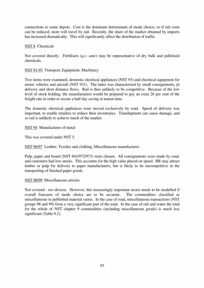
93
connections to some depots. Cost is the dominant determinant of mode choice; so if rail costs
can be reduced, more will travel by rail. Recently, the share of the market obtained by imports
has increased dramatically. This will significantly affect the distribution of traffic.
NST 8 Chemicals
Not covered directly. Fertilisers (q.v. ante) may be representative of dry bulk and palletised
chemicals.
NST 91-93 Transport, Equipment, Machinery
Two items were examined, domestic electrical appliances (NST 93) and electrical equipment for
motor vehicles and aircraft (NST 931). The latter was characterised by small consignments, jit
delivery and short distance flows. Rail is thus unlikely to be competitive. Because of the low
level of stock holding, the manufacturers would be prepared to pay an extra 26 per cent of the
freight rate in order to secure a half day saving in transit time.
The domestic electrical appliances were moved exclusively by road. Speed of delivery was
important, to enable retailers to reduce their inventories. Transhipment can cause damage, and
so rail is unlikely to achieve much of the market.
NST 94 Manufactures of metal
This was covered under NST 5.
NST 96/97 Leather, Textiles and clothing, Miscellaneous manufactures
Pulp, paper and board (NST 841/972/973) were chosen. All consignments were made by road,
and customers had low stocks. This accounts for the high value placed on speed. BR may attract
timber or pulp for delivery to paper manufacturers, but is likely to be uncompetitive in the
transporting of finished paper goods.
NST 98/99 Miscellaneous articles
Not covered - too diverse. However, this increasingly important sector needs to be modelled if
overall forecasts of mode choice are to be accurate. The commodities classified as
miscellaneous in published material varies. In the case of road, miscellaneous transactions (NST
groups 98 and 99) form a very significant part of the total. In the case of rail and water the total
for the whole of NST chapter 9 commodities (including miscellaneous goods) is much less
significant (Table 9.2).
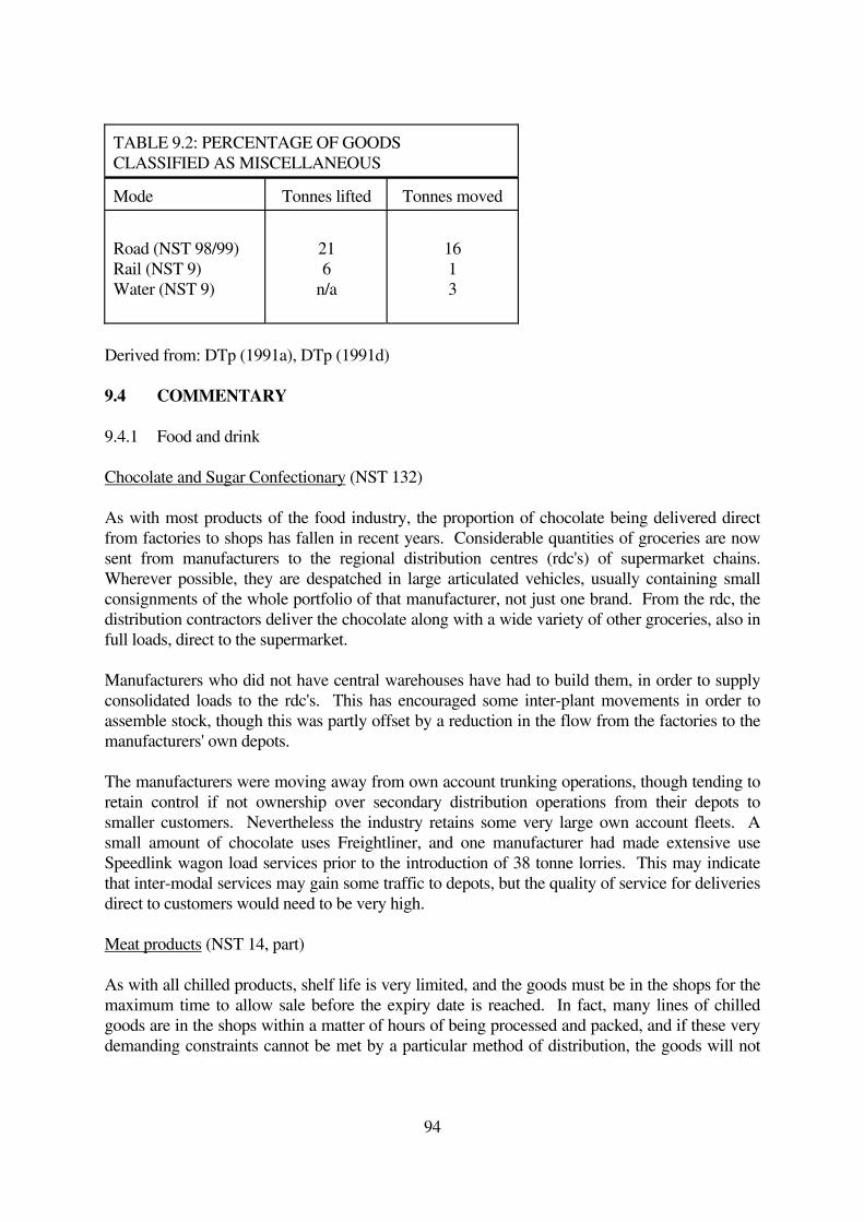
94
TABLE 9.2: PERCENTAGE OF GOODS
CLASSIFIED AS MISCELLANEOUS
Mode Tonnes lifted Tonnes moved
Road (NST 98/99)
Rail (NST 9)
Water (NST 9)
21
6
n/a
16
1
3
Derived from: DTp (1991a), DTp (1991d)
9.4 COMMENTARY
9.4.1 Food and drink
Chocolate and Sugar Confectionary (NST 132)
As with most products of the food industry, the proportion of chocolate being delivered direct
from factories to shops has fallen in recent years. Considerable quantities of groceries are now
sent from manufacturers to the regional distribution centres (rdc's) of supermarket chains.
Wherever possible, they are despatched in large articulated vehicles, usually containing small
consignments of the whole portfolio of that manufacturer, not just one brand. From the rdc, the
distribution contractors deliver the chocolate along with a wide variety of other groceries, also in
full loads, direct to the supermarket.
Manufacturers who did not have central warehouses have had to build them, in order to supply
consolidated loads to the rdc's. This has encouraged some inter-plant movements in order to
assemble stock, though this was partly offset by a reduction in the flow from the factories to the
manufacturers' own depots.
The manufacturers were moving away from own account trunking operations, though tending to
retain control if not ownership over secondary distribution operations from their depots to
smaller customers. Nevertheless the industry retains some very large own account fleets. A
small amount of chocolate uses Freightliner, and one manufacturer had made extensive use
Speedlink wagon load services prior to the introduction of 38 tonne lorries. This may indicate
that inter-modal services may gain some traffic to depots, but the quality of service for deliveries
direct to customers would need to be very high.
Meat products (NST 14, part)
As with all chilled products, shelf life is very limited, and the goods must be in the shops for the
maximum time to allow sale before the expiry date is reached. In fact, many lines of chilled
goods are in the shops within a matter of hours of being processed and packed, and if these very
demanding constraints cannot be met by a particular method of distribution, the goods will not

95
be moved by that method.
In addition, special refrigerated vehicles are required. These factors mean that the chilled traffic
will always use road transport, though rail may gain some of the less perishable frozen and fruit
or vegetable traffic, if it offers a high quality service and provides the special equipment needed.
This may be the case particularly for imported European traffic once the Channel Tunnel is
open.
Brewing (NST 122)
The industry does use rail for some large flows both of finished products to depots, and bulk
movements for packing using ISOtanks on Freightliner trains to canning plants. Deliveries to
customers, which include supermarket rdc's and contractors who deliver to the recently
independent chains of public houses and other outlets, require a much higher level of service.
Constraints which limit the possible penetration of the market by rail are that some traditional
beers have a short shelf life, may be sensitive to temperature and, because they are delivered
along with other brands, the whole product range has a high quality of service. As considerable
quantities of kegs, and to a lesser extent multiple trip bottles, need to be returned for filling,
loading in both directions helps the industry justify very extensive use of own account fleets. In
fact, because the kegs are more valuable than the contents, the transit time of the empties is very
important to minimise barrel inventories.
The closure of Speedlink has seen some major flows lost by rail, since the traffic cannot wait
until a trainload is formed. However, it seems from our survey that inter-modal technology
could gain some traffic in this market, though a high quality of service would be required.
Additionally, the brewers may have to be offered considerable inducements before they dispose
of their own account fleets.
9.4.2 Petroleum products (NST 3)
Large volumes of these products are moved by rail and coastal shipping. The commodity
accounts for virtually all the flows by pipeline of over 25 kilometres. The use of these modes is
mainly due to the volumes which have to be moved from refineries to the consumption areas,
with final delivery being by road, though with direct deliveries to some large industrial users and
power stations. Specialist products, such as lubricating oils and liquid petroleum gas, were much
more likely to be moved to depots or delivered direct to customers by road vehicle.
Because most of the products are held in large stocks, partly to meet statutory requirements and
seasonal fluctuations in demand, the service requirements to depots tended to be low. In fact the
overall result of our survey of the industry indicated that very poor quality services would be
accepted if they reduced costs of trunk movement. This is because the stocks held in the
distribution system allow customer service levels to be maintained.
Suitable inter-modal equipment could be used for the movement of some special products, in
addition to the trunk movement of bulk flows by various modes. Overall, we expect the shift to

96
pipeline to continue, and therefore we cannot see much increase in traffic by either rail or road.
9.4.3 Tubes, pipes and fittings (NST 55)
This commodity ranges from seamless precision steel tubes to large diameter pipes and fittings.
As a result the values and services required show a much greater variation. Many products are
made to order, forming part of the production chain, and needing to meet jit constraints as a
result. Nevertheless, rail had obtained some traffic in the form of large volume trainload flows to
customers. Also, where standard products were made, delivery to depots required a much lower
service requirement than for delivery to customers. This latter traffic is inherently suitable for
rail.
Experience of the use of deep sea containers resulted in the firms being reluctant to use inter-
modal technology which involved lifting the unit. This is because most of the products are
handled in bundles, and damage in the form of dents tends to occur in tubes on the bottom layer
if they are not handled gently.
9.4.4 Cement and lime (NST 64)
This is also representative of low value commodities transported mainly in bulk. The quantities
moving by rail to depots had declined as a result of the collapse of the pricing agreement. Up to
then, the fixed price had led manufacturers to compete on quality of service in each others'
market areas. The new regime discourages manufacturers from shipping an essentially
homogeneous product over long distances, where the reduced price may not be able to cover the
transport costs. Each production plant now tends only to serve its own vicinity. In the last few
years there has also been a significant increase in the quantity of cement imported, usually via a
port close to an area of consumption, minimising the demand for transport services.
Movements to depots were in relatively high volumes, and those flows of over 150 kilometres
which remained generally used rail. Specialist products, such as hydrated lime, tended to be
made at a limited number of plants and distributed nationally by road.
It was felt by interviewees that inter-modal services were not practical for the movement of bulk
cement, and though it was feasible for the smaller flows of bagged products, inter-modal is
unlikely to be cost effective over the short distances involved. Without some unforeseen
technical or regulatory development, the position of rail can be expected to weaken in this sector.
9.4.5 Fertilisers (NST7)
The main problem in this industry is the severe peak in demand, although production takes place
throughout the year. Raw materials (which are mainly imported) and semi-finished fertilisers are
moved all year and require moderate service levels. Movement of stock to depots required only
poor quality services, if costs could be reduced as a result.
Deliveries direct to the farm did demand much better quality services, though as with petroleum
products, stock in the system allowed customer service to be maintained while the costs of trunk
movement could be reduced. Rail does carry significant quantities of this product, but closure of

97
domestic production units and Speedlink will reduce the volume in the short term. Recently, the
share of the market obtained by imports has increased dramatically, with only the finished
product to be distributed in GB. Future projections will depend on whether the domestic
industry can be expected to recover, and whether the imported traffic switches to rail via the
Channel Tunnel.
9.4.6 Electrical goods (NST 93)
Domestic electrical appliances
This range of products is generally of relatively high price and of low density. The most
important transport attribute in our survey was speed of delivery, mainly because retailers in
reducing their inventories put pressure on the supplier to shorten order/lead times. In addition
there was reluctance to allow transhipment of the goods because of the risk of damage.
Given the combination of high service levels, volume constrained loads (only 7-9 tonnes in a 12
metre trailer), and extensive own account road fleets still operated by the manufacturers, rail is
likely to find this a difficult market in which to compete, at least for internal traffic.
Nevertheless, large flows of domestic appliances, especially from Italy, are moved by rail to
Northern France and then transhipped by delivery by road to UK destinations. When the
Channel Tunnel is opened, rail may gain the competitive edge for direct movement, though the
British loading gauge may prove to be a constraint in penetrating this market.
Machinery and electrical equipment
As most of this category of goods form part of the production chain, high quality transport
services are required, especially to serve the automotive industry which is increasingly using jit
production techniques. Additional constraints are imposed because many products are delivered
in relatively small consignments, which are transported in the form of consolidated, or groupage,
loads to minimise costs. It is an area where the smaller vehicle, notably two axle rigids, are used
extensively to provide regular services to customers.
In these circumstances, rail would have difficulty penetrating the market. However, once again
the Channel Tunnel could mean that large volumes of the sub-assemblies used within the
automotive industry could be imported direct by rail. More certain is that a significant
proportion of finished cars and other consumer goods could use the Channel Tunnel.
9.4.7 Pulp, paper and board (NST 841/972/973)
Many of the flows of these commodities form part of the production chain. The high quality of
services required have tended to encourage the use of either own account transport, or contract
distribution. The stocks of the many different grades of product tended to be minimal.
Although this range of products is of moderate value and density, attributes which may make
them attractive for inter-modal techniques, success in penetrating this market would depend
critically on the level of service which could be provided. Basically this must consist of a very
reliable next day delivery service.

98
The input materials to the industry consist of low value timber and pulp. Rail has been more
successful in attracting this traffic, which also tends to be held in relatively large stocks by the
manufacturers, and where the individual flows consist of larger volumes. However, the closure
of Speedlink has hit this traffic hard, since trainload quantities are rare. The above discussion,
together with the long distances often involved, suggest that a more competitive rail freight
operation might regain the lost traffic and even gain more.
9.4.8 Container traffic
In the case of domestic traffic it is reasonable to assume that the requirement in terms of
transport quality is dependent on the commodity rather than the method used. Containerisation
has the advantage of being inter-modal. It also has the disadvantage of offering limited volume
and a higher tare weight when on a road vehicle than orthodox road or rail transport. As a result,
its use has not been very extensive for domestic traffic. Only one domestic Freightliner route has
been a long term commercial success, that from London to Glasgow.
Where the goods are being exported using deep sea, and to a lesser extent short sea, shipping
services, many goods use a container as the unit of transport. In such cases, rail is not at a
disadvantage for the domestic journey to the port in terms of payload restrictions, though length
of haul tends to be relatively short. As the container changes mode at the port however it is
transported there, the use of rail involves only one additional terminal transfer cost.
As a result, Freightliner have been very successful in marketing its services for the carriage of
maritime container traffic. In general, the services are not sold to the shipper of the goods but to
the shipping company offering door to door international services. In some cases the shipping
company, such as P&O, arrange positioning of containers for loading or discharging, and
movement to the Freightliner terminal. The containers are then moved to the major container
ports of Felixstowe, Southampton and Tilbury in trainloads or sections of trains. The system
offers another major advantage in that part of a container vessel's cargo can be moved to Inland
Clearance Depots for customs clearance, and this helps to reduce the congestion at the ports
caused by the speedy unloading of the large container vessels now used for this traffic.
9.5 PROSPECTS FOR MODAL SHIFT
For domestic traffic there is little visible prospect of any large scale modal shift without
regulation and/or government financial incentives. Increased road congestion may make road
transport less reliable, though much of the long distance trunking for which rail is most suited is
carried out overnight. In any case, as a low proportion of trip origins or ends are on the rail
network, some road collection and delivery work is still required, often in the congested urban
areas.
A positive sign is the introduction of various types of new technology in the form of Tiphook
Piggyback and Trailertrain inter-modal services. These are currently being marketed by an
independent company, Charterail, of which British Rail is a major shareholder. This company
has successfully obtained a contract to distribute Pedigree pet foods, some flows of which
require a very high quality of service. If this progress can be maintained, the planned expansion

99
of these services to operate between a network of about seven depots could encourage a shift in
mode for some medium and long distance movements. British Rail's own plans are unclear. A
number of terminals are being equipped to handle new swap body technology for use through the
Channel Tunnel, and this could enable profitable domestic business to be handled if the terminals
have spare capacity.
However, the vast majority of transport movements are fairly short, and inter-modal will be
unable to offer a cost effective service. For longer distances between terminals, and for
distribution of large volumes from a single source (as in the Pedigree case), inter-modal can
obtain traffic where it can offer a quality service package at a cost about the same as road
transport. A combination of the BR loading gauge and the tare weight of some of the equipment
is likely to restrict the range of commodities it can carry efficiently.
Many bulk traffic flows of a large volume already move by modes other than road. It is this
sector of industry which has seen long-term contraction. There is the possibility that rail could
consolidate some flows of such traffic at depots and then trunk them to distribution points, but
this activity is probably not widely applicable.
In recent years the increased imports of bulk materials, including fertiliser, cement and
aggregates, may limit the scope for rail movement of such commodities. It may also indicate
that UK manufacturers are no longer competitive. If this is the case, imports are likely to be via
ports close to the consumers, and the demand for domestic transport may be minimised.
For more general traffic, rail will improve its competitive position for European traffic following
the completion of the Channel Tunnel. This will allow trainloads of commodities and swap
bodies (the inter-modal technology favoured by the railways) to be moved directly across the
continent. Once again the restrictions relating to the BR loading gauge and tare weight of the
equipment apply.
A number of new terminals are planned to handle this traffic. One already in operation is at
Wilton, within a large chemical complex owned by ICI. Moving the terminal to this location
was partly justified because by doing so, containers (and in future swap bodies) could be loaded
to payloads allowed in the destination country, where in general weight limits for road vehicles
are more generous. Containers which are overweight under British law are also exported by ICI
through the Bell Line terminal at Teesport, which can be reached from Wilton without using
public roads. If the vehicle weight and dimensions in Britain and Europe remain less generous
than in other parts of the world, notably North America and the Far East, other large scale
manufacturers may adopt similar strategies to reduce export transport costs.
The question naturally arises, then, as to why rail does not currently have a much larger share of
the market on the continent of Europe where such inter-modal services already operate. We
have not investigated this issue directly, and of course cost conditions may differ from those in
Britain. Nevertheless, discussion with those in industry leave us in little doubt that it is the
failure to achieve a quality of service at all close to that offered by road that is the major
problem. If the railways of Europe can work together to overcome this obstacle, then the
potential of the Channel Tunnel to induce a switch of mode for traffic between Europe and the
UK could have a major impact on this sector of the market.
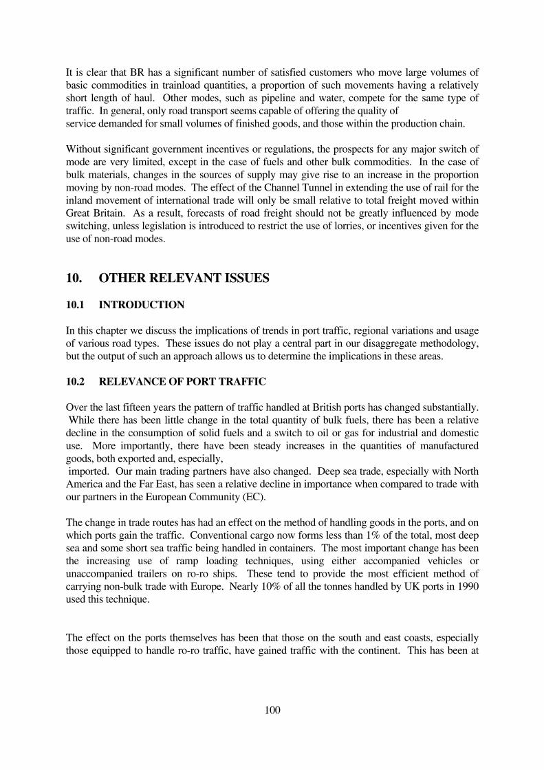
100
It is clear that BR has a significant number of satisfied customers who move large volumes of
basic commodities in trainload quantities, a proportion of such movements having a relatively
short length of haul. Other modes, such as pipeline and water, compete for the same type of
traffic. In general, only road transport seems capable of offering the quality of
service demanded for small volumes of finished goods, and those within the production chain.
Without significant government incentives or regulations, the prospects for any major switch of
mode are very limited, except in the case of fuels and other bulk commodities. In the case of
bulk materials, changes in the sources of supply may give rise to an increase in the proportion
moving by non-road modes. The effect of the Channel Tunnel in extending the use of rail for the
inland movement of international trade will only be small relative to total freight moved within
Great Britain. As a result, forecasts of road freight should not be greatly influenced by mode
switching, unless legislation is introduced to restrict the use of lorries, or incentives given for the
use of non-road modes.
10. OTHER RELEVANT ISSUES
10.1 INTRODUCTION
In this chapter we discuss the implications of trends in port traffic, regional variations and usage
of various road types. These issues do not play a central part in our disaggregate methodology,
but the output of such an approach allows us to determine the implications in these areas.
10.2 RELEVANCE OF PORT TRAFFIC
Over the last fifteen years the pattern of traffic handled at British ports has changed substantially.
While there has been little change in the total quantity of bulk fuels, there has been a relative
decline in the consumption of solid fuels and a switch to oil or gas for industrial and domestic
use. More importantly, there have been steady increases in the quantities of manufactured
goods, both exported and, especially,
imported. Our main trading partners have also changed. Deep sea trade, especially with North
America and the Far East, has seen a relative decline in importance when compared to trade with
our partners in the European Community (EC).
The change in trade routes has had an effect on the method of handling goods in the ports, and on
which ports gain the traffic. Conventional cargo now forms less than 1% of the total, most deep
sea and some short sea traffic being handled in containers. The most important change has been
the increasing use of ramp loading techniques, using either accompanied vehicles or
unaccompanied trailers on ro-ro ships. These tend to provide the most efficient method of
carrying non-bulk trade with Europe. Nearly 10% of all the tonnes handled by UK ports in 1990
used this technique.
The effect on the ports themselves has been that those on the south and east coasts, especially
those equipped to handle ro-ro traffic, have gained traffic with the continent. This has been at

101
the expense of west coast ports (especially Liverpool) which used to handle our deep sea trade,
which have seen a relative decline, and in some cases an absolute decline in traffic. A small
number of ports (Felixstowe, Southampton and Tilbury) have successfully specialised in the
handling of deep sea container trade.
The changes in trade patterns have had an effect on the inland flows of traffic particularly by
road. The success of the major ro-ro ports, Dover and the Haven ports (Felixstowe, Harwich and
Ipswich) in particular, have greatly increased the traffic on the main roads from these ports. The
M2/M20 and A12/A45 corridors have seen large scale infrastructure investment being
outstripped by constant increases in traffic.
10.3 BULK AND SEMI-BULK TRAFFIC
Traffic handled by the ports in bulk, usually a ship carrying only one commodity without any
packaging, has tended to concentrate on a limited number of ports for each traffic. Similarly,
manufacturers who use large volumes of imported raw materials have tended to move their
plants closer to (one or more) ports.
10.3.1 The Major Bulks - Fuel and Iron Ore
Although some crude oil has been exported from terminals such as Sullom Voe and Teesport, the
pattern at major refinery complexes remains that of inbound crude being processed and a large
proportion of the finished products being delivered to their market areas by coastal shipping.
During 1990, Milford Haven received over 15 million tonnes of crude, from which 10 million
tonnes was shipped outward as petroleum products and gas, with over 7m tonnes of this going
for domestic consumption. Other net outward shipments of petroleum products came from
Southampton (3.3mt), the Forth (3.0mt) and Immingham (2.8mt). There were a much larger
number of receiving ports, but the main areas were London and Medway (2.5mt), Bristol
Channel ports (2.7mt), North East Scotland (1.4mt), Tyne and Wear (1.0mt). Given that there
are a number of circuitous shipments by individual companies in supplying their depots, such as
Milford Haven to the Tyne, it is clear that the tonne km figures by coastal shipping are
considerably inflated relative to land transport. It is common in road transport to use a factor of
1.2 when calculating road distance from straight line mileage. For rail, given a more restricted
network a factor of 1.5 may be more appropriate, whereas coastal shipping may require a factor
of the order of 2.5.
In the case of solid fuels, the most important importer is currently British Steel, though
increasing amounts are being brought in by the power generating companies. The integrated
steel plants at Port Talbot and Redcar have direct conveyor links to nearby berths, and coal and
iron ore are fed directly from ship to stock yards. Other plants at Llanwern and Scunthorpe are
fed by rail from Port Talbot and Immingham respectively. The proposed closure of Ravenscraig
would result in the deep water port of Hunterston, which supplied it, becoming available for
other traffic.
Coal is also handled at other ports for domestic and industrial consumption. In the past large
quantities of coal were shipped from South Wales and North Eastern ports, but the only port with
a significant export traffic now is Blyth (0.5mtpa). Most domestic production is moved to power

102
stations by rail, with a small amount using water and the remainder by road. General industrial
and domestic coal movement is mainly carried out by road.
The source of coal for power station consumption may change to imported coal to a much
greater extent over the next decade. As most of the generating stations are located inland, there
would be a requirement for new deep water facilities which are able to handle bulk carriers of up
200,000 tonnes deadweight to enable a cost efficient supply system to be developed.
In the short to medium term, increased coal imports would be likely to increase the demand for
rail movement to the power stations, because the average length of haul will be greater. In the
longer term, new coal fired power stations are likely to be built at or near a point of importation,
eliminating the requirement for domestic transport for coal.
10.3.2 Importation Versus Domestic Production
There are signs which may indicate that the UK economy cannot produce some low value bulk
products cost effectively, at or near the current exchange rate fixed in the Exchange Rate
Mechanism. Evidence of this is shown by the rise in recent years of the import of cement and
fertiliser, and Table 10.1 shows a steady increase in imports of other bulk commodities.
Fertiliser plants were among those which had tended to gravitate towards the ports where their
raw materials arrived, though there is an indigenous source of potash. The chemical industry
supplies the other main ingredients, often in the form of phosphoric acid and ammonia, and some
fertiliser plants were integrated with chemical plants. In this case imports of finished product
merely replaced those of raw materials, and the existing domestic distribution network was little
affected.
TABLE 10.1: IMPORT PENETRATION OF BULK COMMODITIES
(% OF UK CONSUMPTION)
Year 1984 1989 1990
Commodity
Sand, gravel clay
Fertilisers
Chemicals
Cement
Crude materials
0.9
17.0
42.0
3.6
56.0
18.0
1.4
40.0
52.0
20.6
61.0
12.0
68.0
13.0
Source: CSO (1989)
Note: Figures for 1990 are based on estimates from 9 months
The importation of cement may have had a greater effect on the road and rail transport systems.
Domestic production required limestone as a source material, and many plants are located inland.
The finished product was then moved to the main metropolitan consumption areas by either rail
or road. Imported product can be shipped via the port closest to the ultimate destination of the
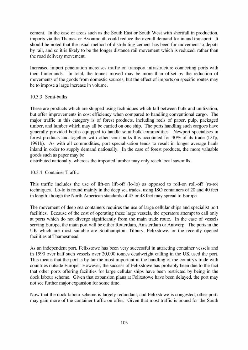
103
cement. In the case of areas such as the South East or South West with shortfall in production,
imports via the Thames or Avonmouth could reduce the overall demand for inland transport. It
should be noted that the usual method of distributing cement has been for movement to depots
by rail, and so it is likely to be the longer distance rail movement which is reduced, rather than
the road delivery movement.
Increased import penetration increases traffic on transport infrastructure connecting ports with
their hinterlands. In total, the tonnes moved may be more than offset by the reduction of
movements of the goods from domestic sources, but the effect of imports on specific routes may
be to impose a large increase in volume.
10.3.3 Semi-bulks
These are products which are shipped using techniques which fall between bulk and unitization,
but offer improvements in cost efficiency when compared to handling conventional cargo. The
major traffic in this category is of forest products, including reels of paper, pulp, packaged
timber, and lumber which may all be carried on one ship. The ports handling such cargoes have
generally provided berths equipped to handle semi-bulk commodities. Newport specialises in
forest products and together with other semi-bulks this accounted for 40% of its trade (DTp,
1991b). As with all commodities, port specialisation tends to result in longer average hauls
inland in order to supply demand nationally. In the case of forest products, the more valuable
goods such as paper may be
distributed nationally, whereas the imported lumber may only reach local sawmills.
10.3.4 Container Traffic
This traffic includes the use of lift-on lift-off (lo-lo) as opposed to roll-on roll-off (ro-ro)
techniques. Lo-lo is found mainly in the deep sea trades, using ISO containers of 20 and 40 feet
in length, though the North American standards of 45 or 48 feet may spread to Europe.
The movement of deep sea containers requires the use of large cellular ships and specialist port
facilities. Because of the cost of operating these large vessels, the operators attempt to call only
at ports which do not diverge significantly from the main trade route. In the case of vessels
serving Europe, the main port will be either Rotterdam, Amsterdam or Antwerp. The ports in the
UK which are most suitable are Southampton, Tilbury, Felixstowe, or the recently opened
facilities at Thamesmead.
As an independent port, Felixstowe has been very successful in attracting container vessels and
in 1990 over half such vessels over 20,000 tonnes deadweight calling in the UK used the port.
This means that the port is by far the most important in the handling of the country's trade with
countries outside Europe. However, the success of Felixstowe has probably been due to the fact
that other ports offering facilities for large cellular ships have been restricted by being in the
dock labour scheme. Given that expansion plans at Felixstowe have been delayed, the port may
not see further major expansion for some time.
Now that the dock labour scheme is largely redundant, and Felixstowe is congested, other ports
may gain more of the container traffic on offer. Given that most traffic is bound for the South
104
East, which is also close to the trade routes followed by deep sea vessels, ship operators will tend
to favour ports in that area.
An alternative method of serving the UK's deep sea container trade is via a continental port.
Some operators of cellular ships prefer only one call in Europe and this tends to be Rotterdam.
This allows the ship to land its cargo as close as possible to the main markets in Germany, the
Benelux countries, and Northern France. The other major market, the UK, is served by short sea
feeder services. Alternatively the containers may be distributed by road and rail, as they are for
Continental destinations. The opening of the Channel Tunnel may encourage this type of
operation.
In addition to feeder services, there are short sea container services to the Continent, Scandinavia
and Baltic ports.
10.3.5 Combined Traffic
In the twenty years to 1990 the number of freight units on ro-ro services increased by a factor of
nine, while the tonnage they carried increased by a factor of twelve. This is the result of the
expansion of trade with our European partners, and the manufacture and distribution of goods on
a Europe-wide basis. However, over the last five years combined traffic with Scandinavia, the
Baltic ports and Iberia has been expanding at a faster rate than with the centre of the EC.
A small amount (less than 1%) of combined transport uses rail and ferry, or barge and ship. Of
the rest 55% is powered goods vehicles (otherwise known as "accompanied") and of this 70%
uses sailings on the Dover Straits. The balance is in unaccompanied trailers, 78% of which use
North Sea crossings.
There are combinations of circumstances which have been largely responsible for this split in
ferry traffic. Accompanied transport tends to be favoured for the movement of high value and
perishable commodities. Much of the latter comes from the southern half of Europe and tend to
use the Dover Straits or English Channel routes. In addition, ferry operators on very short sea
crossings do not want their vessels delayed by loading trailers, which must be pushed on to the
vessel in order to release the traction unit. The "drive through" ferry concept is not suitable for
unaccompanied traffic.
For unaccompanied operations to be successful, efficient use must be made both of the road
equipment and the ferries. As a result the most prominent operators offer an integrated service.
Ferrymasters and Norfolk Line control both elements. Much of the flow is of manufactured
goods between the Midlands, Northern England and Northern Europe, plus Scandinavia. The
traffic on these routes is more closely balanced compared to the carriage of produce, where most
traffic comes from Spain at some periods of the year, whereas at others the traffic is from Italy or
Southern France. In order to make unaccompanied systems cost effective, sufficient traffic for a
regular ferry service of one sailing per day is also required.
Subject to factors such as value, perishability and availability of sailings, combined traffic does
have a tendency to take the most direct route possible. Other factors which influence the choice
of route are the opportunity of using the traction unit and driver for other duties while the trailer
105
is on the ferry, and, particularly where accompanied traffic is concerned, the route chosen may
partly depend on whether the drivers can take their rest period on board the ship. The route and
method chosen is the one perceived to give the best value in terms of cost, speed and reliability
for a particular cargo. Other factors such as security are of less importance. We know of some
Stated Preference studies of relative weights, but feel that little useful is in the public domain.
The two most important ports for combined traffic are firstly Dover, which specialises almost
entirely in accompanied traffic, with some unaccompanied trailers being shipped at night and on
the train ferry. Secondly, the Haven ports, which ship considerable numbers of unaccompanied
trailers, but also offer relatively short sea routes to Northern Europe to attract significant
numbers of accompanied lorries.
Of the other ports, those on the East Coast tend to ship predominantly unaccompanied trailers to
Northern Europe, Scandinavia and Baltic ports. Like Dover, the other Kent ports mainly ship
accompanied traffic. Western Channel ports mainly ship accompanied traffic bound for
Southern Europe. If the traffic in the Western Channel increases and sailings become more
frequent, there may be a switch towards the use of unaccompanied operating methods.
There are signs that Felixstowe may be near capacity for the movement of ro-ro traffic as well as
for containers. The increase in the number of ro-ro units during 1989-1990 was very small,
whereas more peripheral ports such as the Tees and Hull recorded increases of over 20%.
Southampton and Liverpool also increased the number of units handled, in part due to a change
of port by some ferry operators.
10.4 SEABORNE TRADE AND THE EFFECT ON INLAND TRANSPORT
The general pattern is that considerable quantities of bulk commodities are processed directly
within the port, or close to it. In addition, considerable quantities of the finished or semi-finished
goods which result from this process are then shipped from the same port. The main examples
are crude oil being shipped out as petroleum products, and iron ore and coal being converted into
steel products. Of the balance which is not re-exported, rail and pipeline play a considerable role
in the domestic distribution of large volumes of oil and steel products. Industries with direct
access to port facilities, such as Ford at Dagenham and some steel and chemical works on
Teesside, are also able to ship containers and ro-ro units at weights above those allowed within
the UK, as these units do not travel on public roads in this country.
Otherwise virtually all continental traffic uses road for the inland part of its journey. In future
this may change following the introduction of through inter-modal freight services to be offered
by British Rail via the Channel Tunnel. Their forecasts indicate winning up to 10% of the traffic,
which if achieved would remove a significant volume of road traffic currently travelling to the
ports with export traffic from the Midlands and North of England.
Of the deep sea container traffic, considerable numbers of units are moved by Freightliner. The
main routes are from the major container ports of Southampton, Tilbury and Felixstowe to inland
terminals, notably those in Birmingham, Manchester, Leeds and at Coatbridge.
10.5 REGIONAL DISAGGREGATION OF ROAD TRAFFIC

106
Though the demand for movement of some commodities, such as foodstuffs and consumer
goods, is closely related to the size of population this relationship does not hold in all cases. For
this reason, disaggregation by geographic, or standard economic region has been given some
consideration.
Data has been obtained, both published and by correspondence with the DTp, giving the
quantities of commodities dispatched from ,and received into, each region in the U.K., and the
traffic moved within the region. This information highlights the short distance nature of road
transport. Traffic moved inter-regionally is only about one third of that moved intra-regionally.
Consequently regions which specialise in certain commodities will not necessarily follow the
national trends in the movement of goods as a whole.
The economic regions of the U.K. vary in size, and the larger they are the smaller the percentage
of inter-regional traffic is likely to be. Only twelve percent of Scottish originating traffic is
moved inter-regionally. This is almost certainly partially due to large area covered by this region,
with a relatively low population density.
The South East (including Greater London), which has about 30% of the U.K. population, is a
net importer of most commodities, in particular building materials and consumer goods. Many
bulk commodities, such as fuel, are imported into the South East by non-road modes or imported
from other countries direct to ports in the region. The South East also receives large quantities of
basic agricultural products from other areas of the U.K. and abroad (not only from Europe). The
most significant dispatches from the South East to other regions by road are foodstuffs (NST 1
forms 22% of the total), much of which has been processed in the region.
In some cases regions have very large flows of one commodity. This is the result of the existence
of natural resources or of the location of basic industries. In 1990 the East Midlands dispatched
25% of the total cement and lime to be lifted by road, plus 38% of the crude and manufactured
minerals. These commodities formed around 40% of all the tonnes lifted in the region, both for
inter and intra-regional road transport (Table 10.2). Other regions which possess sources of
aggregates, the South West and North West, also have major flows radiating from the quarries.
The relationship between regions other than these and particular groups of commodities are not
so significant. Chemical traffic is dispatched in significant quantities from the North and North
West. Dispatches of steel form over 18% of the inter-regional road traffic from Wales.
One benefit of using a disaggregated forecasting method is that prediction can also be made on a
regional basis, given knowledge of the structural location of industry. Though the movement of
most commodities is widespread, the movement of chemicals, steel and foodstuffs are of
relatively greater importance for a few regions.
Building materials (NST chapter 6) are very important in all regions. However, in the main
production regions of the East Midlands and South West they form over 40% of the dispatches
by road. Nationally they form a third of the tonnes lifted. The data available shows the tonnage
dispatched, but it is not possible to determine accurately the origin and destination regions (or
counties) of these very large flows.

107
Comparison with the situation within the E.C. shows that building materials form 47% of the
tonnes dispatched by road (Eurostat 1991). It would appear that, even though the length of haul
of these materials tends to be short, forecasting the activity in the building sector is most
important to any method of forecasting road freight.

108
TABLE 10.2: PERCENTAGE OF TONNAGE DISPATCHED BY ROAD FROM REGIONS/INTRA-REGIONALLY BY COMMODITY
NST
Chapter
North
Y & H
East
Midlands
East
Anglia
South
East
South
West
Wales
West
Midlands
North
West
Scotland
Northern
Ireland
All
Regions
EUR*
12
(a) Traffic dispatched inter-regionally (%)
0
1
2
3
4
5
6
7
8
9
5.2 7.1
12.4 19.8
9.0 3.9
2.1 2.4
1.9 1.0
7.3 9.6
15.9 15.8
4.4 6.1
10.9 8.0
31.1 26.1
7.4
14.6
3.8
2.5
0.8
4.0
43.0
0.7
2.9
20.3
16.3
26.2
0.2
1.6
0.9
1.2
13.6
0.8
3.8
35.1
11.2
22.0
0.7
3.7
1.5
3.8
11.0
0.7
6.5
38.9
8.4
23.0
0.8
2.5
0.7
1.9
31.5
2.0
4.0
25.2
4.8
13.2
4.4
1.6
0.6
18.4
27.7
0.1
5.3
23.7
5.3
18.8
7.4
3.4
1.8
7.4
19.6
0.3
2.7
33.1
4.8
20.7
1.2
5.5
1.5
4.6
12.8
1.1
15.4
32.4
12.6
21.9
6.8
1.1
0.9
6.3
4.9
0.7
8.3
36.4
13.7
36.0
1.4
0.4
0.1
1.8
4.8
0.1
2.2
39.3
7.7
19.0
3.5
2.9
1.2
6.0
21.1
1.7
6.8
29.6
7.6
11.9
2.0
4.7
1.3
2.3
47.7
1.2
5.1
16.2
(b) Intra-regional traffic (%)
0
1
2
3
4
5
6
7
8
9
1.8 5.9
7.0 13.2
8.9 5.8
2.2 4.0
0.7 1.3
2.2 6.1
36.9 26.3
1.8 0.6
4.2 4.0
34.1 32.3
5.5
10.7
12.0
2.6
0.8
0.9
38.9
0.3
1.8
26.5
22.2
13.7
0.6
3.4
0.2
1.0
31.1
0.7
1.3
25.7
4.1
11.2
0.3
5.2
0.9
0.7
37.1
0.3
2.1
38.0
4.7
17.8
0.6
6.7
0.2
1.1
45.8
1.3
1.1
20.4
3.0
9.4
11.3
3.1
1.6
6.1
41.9
1.5
1.7
19.9
3.1
9.0
2.6
5.7
0.5
5.4
35.9
0.2
0.5
36.8
4.0
14.4
1.3
6.7
1.2
1.8
29.7
0.1
6.3
33.9
6.7
14.5
4.7
6.0
1.6
2.6
30.2
0.5
1.5
31.1
7.3
14.4
5.3
6.3
0.3
1.7
43.6
2.9
1.7
16.3
5.4
12.2
3.9
5.0
0.9
2.5
35.3
0.6
2.5
31.2
(c) Percentage of population
5 9 7 4 30 8 5 9 11 9 3 101

109
Source: derived from Carriage of Goods, Road 1989. Eurostat, Theme 7C, Luxemburg. Annual Abstract of Statistics 1991. HMSO, London. Private
Correspondence with DTp.
Note: (*) figures for EUR12 refer to 1989 and include intra-regional road freight. Other columns give 1990 figures.

110
10.6 CHANGES IN USE OF CATEGORIES OF ROADS
In overall terms commercial vehicle traffic, measured as vehicle kilometres, has increased on all
types of road, but has not expanded as quickly as car traffic. The forecasts of commercial
vehicle traffic are thus of declining importance in the calculation of total traffic.
However, the proportional re-distribution of vehicle use by road category has been uneven
(Table 10.3). The extensive use of the Motorway and rural trunk road network by both small and
heavy goods vehicles has resulted in them becoming more significant categories on the strategic
road network. Once again this is partly due to the use of larger vehicles on trunk hauls, and to
time sensitive high quality services in all sizes of vehicle.
The major growth in traffic has been in private motoring, particularly in urban areas. As a result
commercial vehicle traffic has increased in significance on inter-urban roads, but its proportion
of the total on urban roads has fallen by a quarter in ten years.
TABLE 10.3: VEHICLE KILOMETRES BY VEHICLE AND ROAD TYPE
(PER 1000 VEHICLE KILOMETRES)
Year: 1975 1980 1985 1990
Vehicle: SGV HGV SGV HGV SGV HGV SGV HGV
Motorway
Built up
Trunk
Principal
Non built up
Trunk
Principal
Minor
All roads
5.1
42.8
38.9
n/a
86.8
16.2
26.0
37.9
n/a
80.2
6.2
3.3
14.9
9.1
10.6
35.3
79.4
17.0
3.2
11.0
14.7
11.1
17.8
74.8
9.9
2.4
17.0
11.4
11.5
29.9
82.1
21.8
2.4
10.1
18.4
11.4
11.8
76.0
12.2
2.3
14.3
12.0
12.2
35.7
88.7
21.5
1.9
8.2
15.7
9.2
16.1
72.6
Source: derived from Transport Statistics Great Britain (various years), HMSO, London.
There have been changes within the categories of commercial vehicles. SGV's doubled their
proportion of vehicle kilometres on motorways during the 1980's. Two axle rigid vehicles also
increased proportionately on motorways. The other main change was in the proportion of total
vehicle kilometres run by the largest articulated vehicles on the strategic road network. The use
of such vehicles was encouraged by the introduction of the 38 tonne GVW lorry in 1983.
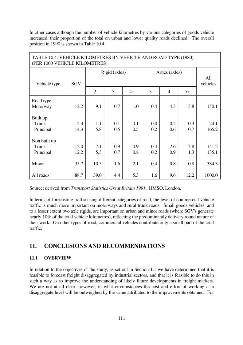
111
In other cases although the number of vehicle kilometres by various categories of goods vehicle
increased, their proportion of the total on urban and lower quality roads declined. The overall
position in 1990 is shown in Table 10.4.
TABLE 10.4: VEHICLE KILOMETRES BY VEHICLE AND ROAD TYPE (1980)
(PER 1000 VEHICLE KILOMETRES)
Vehicle type
SGV
Rigid (axles) Artics (axles)
All
vehicles
2 3 4+ 3 4 5+
Road type
Motorway
Built up
Trunk
Principal
Non built up
Trunk
Principal
Minor
All roads
12.2
2.3
14.3
12.0
12.2
35.7
88.7
9.1
1.1
5.8
7.1
5.3
10.5
39.0
0.7
0.1
0.5
0.9
0.7
1.6
4.4
1.0
0.1
0.5
0.9
0.8
2.1
5.3
0.4
0.0
0.2
0.4
0.2
0.4
1.6
4.3
0.2
0.6
2.6
0.9
0.8
9.6
5.8
0.3
0.7
3.8
1.3
0.8
12.2
150.1
24.1
165.2
141.2
135.1
384.3
1000.0
Source: derived from Transport Statistics Great Britain 1991. HMSO, London.
In terms of forecasting traffic using different categories of road, the level of commercial vehicle
traffic is much more important on motorways and rural trunk roads. Small goods vehicles, and
to a lesser extent two axle rigids, are important on urban and minor roads (where SGV's generate
nearly 10% of the total vehicle kilometres), reflecting the predominantly delivery round nature of
their work. On other types of road, commercial vehicles contribute only a small part of the total
traffic.
11. CONCLUSIONS AND RECOMMENDATIONS
11.1 OVERVIEW
In relation to the objectives of the study, as set out in Section 1.1 we have determined that it is
feasible to forecast freight disaggregated by industrial sectors, and that it is feasible to do this in
such a way as to improve the understanding of likely future developments in freight markets.
We are not at all clear, however, in what circumstances the cost and effort of working at a
disaggregate level will be outweighed by the value attributed to the improvements obtained. For

112
example, if only national level aggregate forecasts of road traffic were required, substantial
forecasting error must be allowed for no matter how the forecasting is done, and any reduction of
this error due to an improved freight forecasting method may be of little value for that purpose.
In this chapter we shall make recommendations mainly of a technical nature regarding how to
take forward an evaluation of disaggregate freight forecasting, but our main recommendation is
that this direction will be a fruitful one to follow.
11.2 WHAT DECISIONS ARE THE FORECASTS MEANT TO INFORM?
The Department of Transport has wide ranging uses for freight forecasts which should not be
oversimplified here. However, those uses that are regarded as absolute requirements, such that
substantial efforts can be devoted to their provision, are much fewer.
Firstly, the Department has to forecast future road use, principally in connection with the road
building programme. Currently the forecasts of future car ownership and use are constructed by
a complex procedure taking several explanatory factors into account. By contrast, forecasts of
hgv use are taken to rise in direct proportion to GDP, ie. with unit elasticity. However, it is not
just the number of hgv's which is important. The size and axle-weights of hgv's are even more
important. Under- or over-provision of road space or strength could be a costly misuse of
resources. Hence, even if disaggregate freight forecasting had little to offer in terms of
noticeably smaller forecast error intervals around the volume of traffic, improved forecasts of
pcus and standard axles could still be worth having.
Secondly, the Department continues to vet large investment expenditures by British Rail, acting
somewhat in the role of the shareholders of a private company. In particular, the movement of
freight by rail requires large capital investments both in infrastructure and rolling stock. The
Department has to give approval for large investments by BR, and may give a `Freight Facilities
Grant' to BR's customers. The Department may be working to a `Level Playing Field' plan of
fair treatment of modes, or may be seeking ways of achieving ministerial aspirations of a
diversion of freight from road to rail. In either case the Department will wish to judge the
wisdom of any rail freight investment it is asked to sanction. Aggregate forecasts will be of little
use in this regard. Disaggregated forecasts of sectoral freight movements, together with an
indication of likely mode choice under various conditions, would greatly assist in such decisions.
11.3 FINDINGS AND RECOMMENDATIONS REGARDING DATA SOURCES
We experienced much greater difficulty and delay in obtaining suitable data than we had been
led to expect. Partly this resulted from genuine non collection/collation of data which one would
hardly credit not to be easily available, and partly we were sometimes viewed as low priority by
those charged with providing us with the data that was available. Obviously, there will always
be an important cost dimension when considering data provision, but full advantage should be
taken of opportunities to collate data already required for other purposes, and to more fully
exploit the responses to surveys undertaken for other reasons.
Specifically we make the following recommendations.
11.3.1 That the next major review of CSRGT data handling should seek to provide an origin-

113
destination matrix for roadfreight by tonnes disaggregated by broad commodity sector (eg. NST
chapter headings, or the more recent 24 way split). The normal degree of confidentiality must
obviously be respected. In aid of this it is proposed that the geographic breakdown be into
regions, but with county to county flows shown within regions. Furthermore, we recommend
that figures published or otherwise made available should not be those from a given year's
CSRGT, but an exponentially smoothed series, updated quarterly. With these two concessions to
confidentiality, coupled with the imprecision due to normal sampling variability we can see no
objection to the production of this valuable data source, at minimal marginal cost.
11.3.2 The problem posed by the expanding `miscellaneous' category in CSRGT should be
tackled by periodic samples of the returns so as to code them to a much finer detail. The
remaining `miscellaneous' returns would then be allocated pro-rata to this sample. A (much
smaller) miscellaneous category would no doubt remain, but proper attribution of mixed loads
should give a much better commodity breakdown, particularly for judging changes over time.
11.3.3 We recommend that, a further improvement to the treatment of CSRGT replies should
be obtained by better categorisation of vehicles. In particular, the recent growth in `curtain-
sided' vehicles is completely lost in the figures, being classified as `other'.
11.3.4 The EC impose data collection and provision requirements in addition to those arising
out of the needs of the Department and BR. We recommend that this be used as an opportunity
to develop new high quality data for all freight traffic on all modes at little additional cost.
While this might in part involve collection of such additional data that now becomes cost
effective given the data collection effort for the EC, we are also concerned that greater attention
be given to quality control. Our investigations have led us to suspect that the rail data supplied to
the EC is particularly poor.
11.3.5 Where changes of method of data collection are made we recommend that the
Department ensure that statistical series can be preserved, preferably by continuing to publish
series on the old basis, but at least by giving advice as to the effect of the change in one `overlap'
year.
11.4 FINDINGS AND RECOMMENDATIONS REGARDING MODELLING
Generally our modelling work has proceeded well, given the limitations of the data sources.
Clearly, the passage of time will allow longer data series to build up, provided that a proper
overlap period/advice is given whenever there is any change to the data collection method. We
accept that there are difficulties and that sometimes the benefits of modelling at the disaggregate
level will not outweigh the costs. Nevertheless, in this feasibility study we believe that we have
demonstrated sufficiently that the opportunities are there, and we now make recommendations
on how these may be investigated further.
11.4.1 We recommend that our unexpected findings as regards handling factors and lengths of
haul be further investigated. We would hope to publish our work as one means of stimulating
debate in this area. Projection of handling factors and haul lengths could be a very valuable
cross check on other disaggregate forecasting procedures, ie. in checking that all the projections
`hang together'. The weight of conviction carried by forecasts from a disaggregate econometric

114
forecasting equation would be greatly strengthened if projections of handling factors and haul
lengths were in agreement with them.
11.4.2 We recommend that the econometric modelling begun in this project, and reported in
Chapter 4, be taken further. Our results could form the basis of a discussion in the profession of
how to proceed. Again, publication of our results might be a vehicle for this. We have our own
further ideas which have not been subjected to proper test and scrutiny due to time constraints on
this project. Wherever possible, however, we have tried to include the better thought out new
ideas in the text even where it has not been possible to apply them as widely as might have been
hoped.
11.4.3 We recommend that the offer of Cambridge Econometrics to provide old sectoral output
forecasts for use in testing our sectoral freight forecasting equations against an aggregate forecast
be taken up. To provide a fair test the forecast of GDP would be the same in each case, with
sectoral outputs adjusted to suit. We had hoped to undertake this work during the project, but
Cambridge Econometrics were too busy to supply the data.
11.5 THE VALUE OF DISAGGREGATE FREIGHT FORECASTING
We had no illusions when we began this project that there would be considerable difficulties.
We clearly overestimated the amount of data which we would be able to obtain, but we see no
reason why this should be held against disaggregate freight forecasting, since the relevant data
should be available to the Department should it wish to take these methods further. It is now our
view that this feasibility study has demonstrated that there are worthwhile benefits to be had.
As one example we would cite the ease of incorporating information on future structural changes
in a particular sector (eg. closure of Ravenscraig, rapid reduction in GB deep mining) into a
disaggregate forecasting system. Secondly, given projections of future attributes of the various
freight modes, a disaggregate system should allow a much improved forecast of future mode
split, and indicate what effect policies designed to modify this will have. Thirdly, the thrust of
our econometric work points to the potential of producing forecasts of national lorry use with
smaller error ranges than those resulting from the aggregate approach. Furthermore, by
considering the type of vehicles likely to be favoured by each sector, the disaggregate method
should give a better projection of pcus and standard axles. We cannot imagine that the extra cost
of producing disaggregate freight forecasts will be at all large, relative to the Department's
expenditures based on decisions which such forecasts might better inform.

115
ANNEX 1: CROSS-CLASSIFICATION OF COMMODITY CODINGS
Groups
of goods
NST/R
chapter
NST/R
group
SIC
SITC
division
Description
1
2
3
4
5
0
0
0
0
0
01
02 03
00 06
05
04 09
001 211
001 218
001
461-463
431-435
04
05
00 06
24
21 23 26
29 44
Cereals
Potatoes, other fresh or frozen fruit and vegetables
Live animals, sugar beet (NB CSRGT uses 08 for
live animals)
Wood and cork
Textile, textile articles and manmade fibres, other
raw animal and vegetable materials
6
7
1
1
11-14
16-17
18
217 229 412-415
420-429
423
01-05
07-09
11 12
09 41-43
Foodstuffs and animal fodder
Oil seeds and oleaginous fruit and fats
8 2 21-23 11-12 32 Solid mineral fuels
9
10
3
3
31
32-34
13
14
33
33 34
Crude petroleum
Petroleum products
11
12
4
4
41 46
45
21
21
28
28
Iron ore, iron and steel waste and blast furnace dust
Non-ferrous ores and waste
13 5 51-56 221-224 67-69 Metal products
14
15
6
6
64 69
61-63
65
241 242
231 233 233 241
243
66
27 66
Cement, lime, manufactured building materials
Crude and manufactured materials
16 7 71 72 256 27 56 Natural and chemical fertilisers
17
18
19
8
8
8
83
81 82
89
84
251
251 257 258 329
483
471
33
51-55
57-59
25
Coal chemicals, tar
Chemicals other than coal chemicals and tar
Paper pulp and waste
20
21
22
23
24
9
9
9
9
9
91-93
94
95
96 97
99
32 34-36
31
247
451-455 465 467
471 472 475 481
464 491
495
71-79
69
66 81
61-65
82-85
63 89
90
Transport equipment, machinery, apparatus, engines,
whether or not assembled, and parts thereof
Manufacturers of metal
Glass, glassware, ceramic products
Leather, textile, clothing, other manufactured articles
Miscellaneous articles (NB CSRGT uses 88 for parcels,
98 for arms and ammunition, and codes these as well as

116
commodity "not known" as miscellaneous)
The Nomenclature Statistique de Transport (NST) was developed from the Commodity
Classification for Transport Statistics in Europe which was prepared by the UNO. The
Standard Industrial Classification (SIC) is used by the Department of Trade and Industry,
Central Statistics Office, and the Business Statistics Office as a means to classify industrial
output. The Standard International Trade Classification (SITC) is used by Customs and
Excise for commodity entries and statistics.
ANNEX 2: RESULTS OF REGRESSIONS ON SECTORAL OUTPUT AND GDP
Results are reported first for "tonnes lifted" models and then for "tonne-kilometres moved"
models. Where a lagged structure was employed, this is indicated in the rubric and the
elasticities reported are long-run. For linear models, the elasticities are based on 1989 figures.
We also indicate how good the models were at predicting tonnes lifted and tonne-kms moved for
1990 when given the output and GDP indices for that year. Fuller details of the models and their
predictive abilities are to be found in tables 4.2 and 4.3 at the end of chapter 4. We also report
the results of aggregate models of the whole economy.
NST 0 and 1 (combined) Agriculture and foodstuffs
Autocorrelation was not a problem with these models, and so a lagged structure is not
appropriate or necessary. The sectoral output (Output) models using tonnes lifted (T) as the
dependent variable gave sensible elasticities, but with a relatively poor fit, explaining just over
40% of the variation in the data:
Double log: EL(T, Output) = 0.72 (s.e. = 0.23)
Linear: EL(T, Output) = 0.75 (ȕ = 2.05, s.e. = 0.636)
Models with tonne-kms (K) as the dependent variable explained 88% of the variation in the data,
and gave high and significant elasticities:
Double log: EL(K, Output) = 3.14 (s.e. = 0.314)
Linear: EL(K, Output) = 2.81 (ȕ = 0.8, s.e. = 0.079)
The high elasticities are rather disturbing and unexpected.
The models using GDP as the independent variable had a better fit. Autocorrelation was not a
problem with these models, and so a lagged structure is not appropriate or necessary.
The models using tonnes lifted as the dependent variable gave low elasticities and explained just
under 50% of the variation in the data:
Double log: EL(T, GDP) = 0.29 (s.e. = 0.083)
Linear: EL(T, GDP) = 0.33 (ȕ = 0.84, s.e. = 0.23)
Models with tonne-kms as the dependent variable explained 93% of the variation in the data, and
gave significant elasticities of a little over unity.
Double log: EL(K, GDP) = 1.23 (s.e. = 0.093)

117
Linear: EL(K, GDP) = 1.19 (ȕ = 0.317, s.e. = 0.022)
The 95% confidence limits on point prediction were quite narrow, mostly within +/- 10%.

118
NST 04 Crude materials
The sector output models were poor, with low explanatory power (R2 of around 0.25 for the
tonnes lifted models, 0.16 for tonne-kms), though with marginally significant parameter
estimates. The elasticities were high for tonnes lifted, but much lower for tonne-kms moved.
Double log: EL(T, Output) = 1.73 (ȕ = 1.729, s.e. = 0.700)
Linear: EL(T, Output) = 2.70 (ȕ = 0.391, s.e. = 0.180)
Double log: EL(K, Output) = 0.43 (s.e. = 0.426)
Linear: EL(K, Output) = 0.40 (ȕ = 0.007, s.e. = 0.004)
The GDP based models had a much better fit for tonnes lifted (R2 about 0.7), but much of the
explained variation was due to the incorporation of a lag; the parameter on GDP was
insignificant.
Double log: EL(T, GDP) = 0.72 (ȕ = 0.373, s.e. = 0.375)
Linear: EL(T, GDP) = 0.41 (ȕ = 0.040, s.e. = 0.054)
The tonne-kms moved models also included a lag, but were not noticeably better than their
sectoral output counterparts.
Double log: EL(K, GDP) = 0.38 (ȕ = 0.200, s.e. = 0.302)
Linear: EL(K, GDP) = 0.47 (ȕ = 0.004, s.e. = 0.005)
The sectoral output models predicted the 1990 outturn better than the GDP models, but the
tonnes lifted models had very high confidence intervals; +/- 123% for the linear model. The
sectoral tonne-kms moved had confidence limits of about +/- 25%.
NST 05 Wood, timber and cork
The sectoral output models were poor, even though a lag was used. The tonnes lifted models had
R2 of 0.22 and completely insignificant parameter estimates.
Double log: EL(T, Output) = -0.02 (ȕ = -0.005, s.e. = 0.263)
Linear: EL(T, Output) = 0.03 (ȕ 0.004, s.e. = 0.064)
The tonne-kms moved models had higher R2, but still had insignificant elasticities.
Double log: EL(K, Output) = 0.16 (ȕ = 0.051, s.e. = 0.348)
Linear: EL(K, Output) = 0.26 (ȕ = 0.002, s.e. = 0.009)
The GDP models had higher elasticities and more significant parameter estimates. Again, a lag
was used.
Double log: EL(T, GDP) = 0.81 (ȕ = 0.445, s.e. = 0.274)
Linear: EL(T, GDP) = 0.87 (ȕ = 0.101, s.e. - 0.058)
Double log: EL(K, GDP) = 1.42 (ȕ = 1.141, s.e. = 0.406)
Linear: EL(K, GDP) = 1.37 (ȕ = 0.028, s.e. = 0.009)

119
The predictive abilities of these models was poor, all models substantially overestimating the
1990 outturn; indeed, the 1990 result lay outside the confidence limits of the tonnes lifted GDP
models.
NST 2 Coal and coke
The sector output models were relatively poor. Autocorrelation was present in the models with
tonnes lifted, and so a lag was used. 40 to 50% of the variation was explained. The demand
appears surprisingly inelastic.
Double log: EL(T, Output) = 0.14 (ȕ = 0.205, s.e. = 0.063)
Linear: EL(T, Output) = 0.13 (ȕ = 0.128, s.e. = 0.047)
For tonne-kilometres moved, the models produced negative elasticities. The large structural
changes in the coal industry over the period mean the models are unreliable, reflecting trends
which cannot continue. There is also the problem of road being very much a minority mode for
coal transport. The tonne-kms models were not lagged, and had R2 0.27 (double-log) and 0.4.
Double log: EL(K, Output) = -0.39 (s.e. = 0.17)
Linear: EL(K, Output) = -0.46 (ȕ = -0.015, s.e. = 0.005)
Attempts were made to improve the reliability of the models by incorporating a dummy for
1984, the year of the miners' strike. This had the effect of reducing the significance of the
parameters in the tonnes lifted models, but substantially increasing the explanatory power of the
tonne-kms moved models, which then had more extreme and more significant negative
elasticities.
The GDP models were mixed. Autocorrelation was present in the models with tonnes lifted, and
so a lag was used. Little of the variation was explained, about 15%. The elasticities were wrong
sign and insignificant.
Double log: EL(T, GDP) = -0.13 (ȕ = -0.189, s.e. = 0.202)
Linear: EL(T, GDP) = -0.13 (ȕ = -0.124, s.e. = 0.139)
For tonne-kilometres moved, the models produced were better than those with sector output as a
dependent variable. They were not lagged, and had R2 of around 0.63. These models are clearly
better than the sectoral output models.
Double log: EL(K, GDP) = 1.37 (s.e. = 0.282)
Linear: EL(K, GDP) = 1.24 (ȕ = 0.044, s.e. = 0.009)
The 95% confidence bands were quite wide, although the best models had a range of +/- 20%.
The outturn was well within the prediction confidence limits.
The figures of freight moved by road in this sector do not tell the full story. In 1990, rail
accounted for 52% of tonnes lifted and 54% of tonne-kms moved. Incorporating coal moved by
rail and water gave even worse models with GDP as the independent variable; but the models
based on sectoral output were much better. There was no autocorrelation, so unlagged models
were used. For tonnes lifted, the models achieved R2 of 0.88 for the linear model and 0.93 for

120
the double-log model. The parameter estimates were highly significant.
Double log: ELall-modes(T, Output) = 0.68 (s.e. = 0.05)
Linear: ELall-modes(T, Output) = 0.63 (ȕ = 0.865, s.e. = 0.089)
The tonne-kms models had R2 of 0.68 for the linear model and 0.8 for the double log. The
parameter estimates were again significant, but less so than those in the tonnes lifted models.
Double log: ELall-modes(K, Output) = 0.72 (s.e. = 0.1)
Linear: ELall-modes(K, Output) = 0.60 (ȕ = 0.060, s.e. = 0.011)
It remains to be seen whether increasing imports of coal will reduce the usefulness of the sectoral
output models.
NST 3 Petroleum products
There were no significant autocorrelation problems, but the explanatory power of the models is
only about 40%. The tonnes lifted models had elasticities close to unity.
Double log: EL(T, Output) = 1.00 (s.e. = 0.322)
Linear: EL(T, Output) = 0.97 (ȕ = 0.67, s.e. = 0.23)
The parameters are slightly more significant in the tonne-kms models.
Double log: EL(K, Output) = 0.76 (s.e. = 0.259)
Linear: EL(K, Output) = 0.76 (ȕ = 0.03, s.e. = 0.01)
The GDP models of tonnes lifted had wrong-sign and insignificant elasticities.
Double log: EL(T, GDP) = -0.58 (ȕ = -0.302, s.e. = 0.326)
Linear: EL(T, GDP) = -0.71 (ȕ = -0.212, s.e. = 0.241)
With the tonne-kms models, there were autocorrelation problems, necessitating a lag, and the
explanatory power of the models was weak, about 18%. The parameters are insignificant.
Double log: EL(K, GDP) = 0.15 (ȕ = 0.091, s.e. = 0.269)
Linear: EL(K, GDP) = 0.18 (ȕ = 0.004, s.e. = 0.012)
The confidence bands were wide, around +/- 20% for the sectoral models, and over +/- 25% for
the GDP models. The predictions were, though, quite close to the outturn.
These data omit transport of petroleum products by water, which is a significant mode in this
sector. This is because much of the traffic is seaborne from the oilfields to the ports, and
therefore not relevant to freight on the mainland. However, we did add rail and pipeline
movements to see if the models could be improved. In 1990, pipeline accounted for about 60%
of tonnes lifted and tonne-kms moved. There are problems with the data series for pipeline
traffic, since the basis for calculating traffic changed.
The sectoral output models were not very good, in fact even worse than the models of road
freight. This may well be due to changes in North Sea Oil production, which was only just

121
coming on stream at the start of the period; production plus imports may have been a better
independent variable. However, the models based on GDP were better. All required a lag to
remove autocorrelation. The tonnes lifted models achieved R2 of 0.2; not very good, but the
parameters were right sign (though insignificant).
Double log: ELall-modes(T, GDP) = 0.08 (ȕ = 0.044, s.e. = 0.202)
Linear: ELall-modes(T, GDP) = 0.07 (ȕ = 0.057, s.e. = 0.338)
The tonne-kms models had R2 in excess of 0.44.
Double log: ELall-modes(K, GDP) = 0.41 (ȕ = 0.221, s.e. = 0.272)
Linear: ELall-modes(K, GDP) = 0.37 (ȕ = 0.030, s.e. = 0.041)
NST 4 Ores
Very poor road models all round, with insignificant parameters and low R2. The tonnes lifted
models had R2 of about 0.15, partly, but not solely, due to the incorporation of a lag.
Double log: EL(T, Output) = 0.37 (ȕ = 0.50, s.e. = 0.44)
Linear: EL(T, Output) = 0.46 (ȕ = 0.09, s.e. = 0.07)
The tonne-kms models had no autocorrelation, but explained almost none of the variation in the
data, R2 = 0.04.
Double log: EL(K, Output) = 0.40 (s.e. = 0.53)
Linear: EL(K, Output) = 0.43 (ȕ = 0.04, s.e. = 0.005)
GDP as the independent variable produced reasonable models all round, with significant
parameters and R2 of 0.34 to 0.38. The tonne models had autocorrelation, so a lag was
employed.
Double log: EL(T, GDP) = 0.55 (ȕ = 0.775, s.e. = 0.325)
Linear: EL(T, GDP) = 0.59 (ȕ = 0.132, s.e. = 0.059)
The tonne-kms models also had a lag.
Double log: EL(K, GDP) = 1.00 (ȕ = 1.260, s.e. = 0.470)
Linear: EL(K, GDP) = 0.98 (ȕ = 0.013, s.e. = 0.005)
Although the confidence bands were sometimes wider than +/- 35%, the prediction was usually
less than 10% away from the actual 1990 figure.
Again, the road figures do not tell the full story. In 1990, rail accounted for 33% of tonne=kms
moved. (Figures for tonnes lifted were not available for this group of commodities.) As with
petrol and oil, the sectoral output models of freight movement by all modes were worse than the
road freight models. This is likely to be due to the omission of imports; output plus imports may
have been better. The GDP models, though, were much better than the road freight models. No
lag was necessary, and R2 in excess of 0.6 were achieved.
Double log: ELall-modes(K, GDP) = 1.21 (s.e. = 0.27)
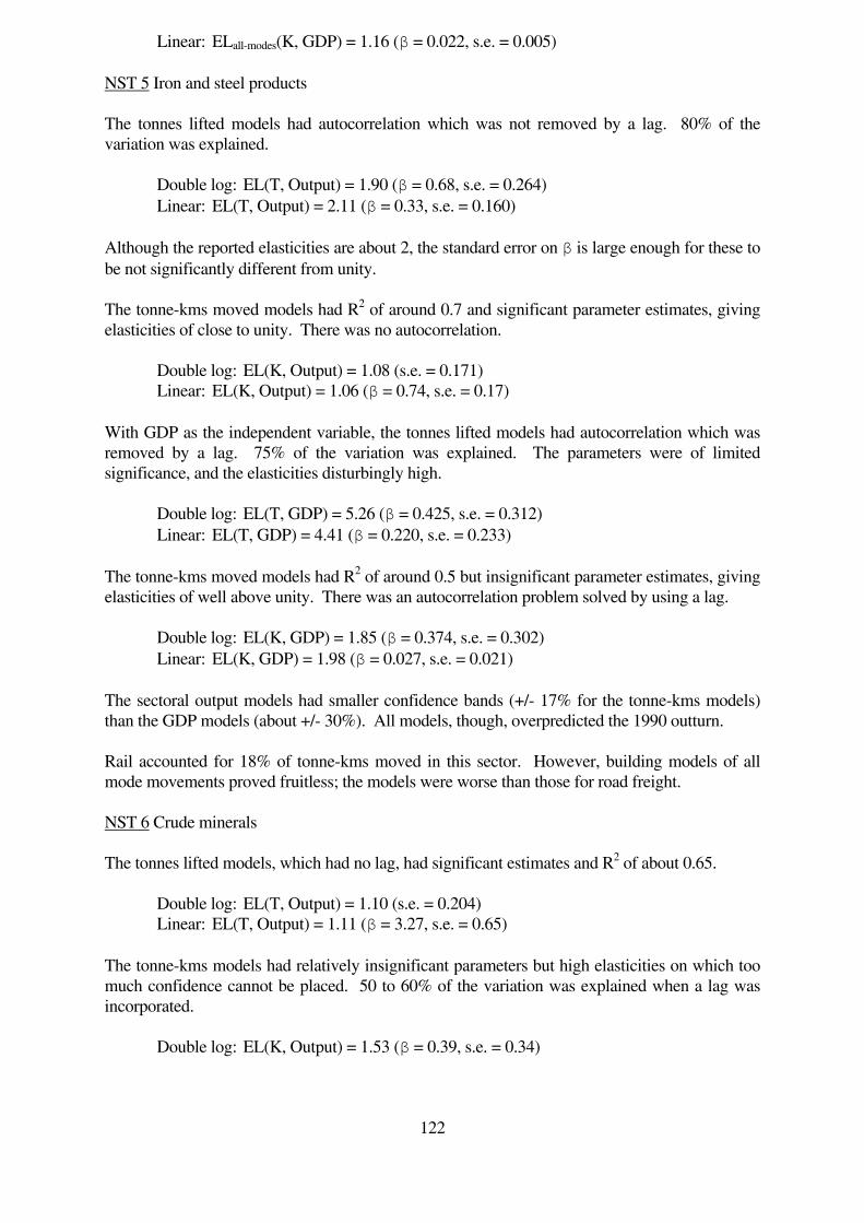
122
Linear: ELall-modes(K, GDP) = 1.16 (ȕ = 0.022, s.e. = 0.005)
NST 5 Iron and steel products
The tonnes lifted models had autocorrelation which was not removed by a lag. 80% of the
variation was explained.
Double log: EL(T, Output) = 1.90 (ȕ = 0.68, s.e. = 0.264)
Linear: EL(T, Output) = 2.11 (ȕ = 0.33, s.e. = 0.160)
Although the reported elasticities are about 2, the standard error on ȕ is large enough for these to
be not significantly different from unity.
The tonne-kms moved models had R2 of around 0.7 and significant parameter estimates, giving
elasticities of close to unity. There was no autocorrelation.
Double log: EL(K, Output) = 1.08 (s.e. = 0.171)
Linear: EL(K, Output) = 1.06 (ȕ = 0.74, s.e. = 0.17)
With GDP as the independent variable, the tonnes lifted models had autocorrelation which was
removed by a lag. 75% of the variation was explained. The parameters were of limited
significance, and the elasticities disturbingly high.
Double log: EL(T, GDP) = 5.26 (ȕ = 0.425, s.e. = 0.312)
Linear: EL(T, GDP) = 4.41 (ȕ = 0.220, s.e. = 0.233)
The tonne-kms moved models had R2 of around 0.5 but insignificant parameter estimates, giving
elasticities of well above unity. There was an autocorrelation problem solved by using a lag.
Double log: EL(K, GDP) = 1.85 (ȕ = 0.374, s.e. = 0.302)
Linear: EL(K, GDP) = 1.98 (ȕ = 0.027, s.e. = 0.021)
The sectoral output models had smaller confidence bands (+/- 17% for the tonne-kms models)
than the GDP models (about +/- 30%). All models, though, overpredicted the 1990 outturn.
Rail accounted for 18% of tonne-kms moved in this sector. However, building models of all
mode movements proved fruitless; the models were worse than those for road freight.
NST 6 Crude minerals
The tonnes lifted models, which had no lag, had significant estimates and R2 of about 0.65.
Double log: EL(T, Output) = 1.10 (s.e. = 0.204)
Linear: EL(T, Output) = 1.11 (ȕ = 3.27, s.e. = 0.65)
The tonne-kms models had relatively insignificant parameters but high elasticities on which too
much confidence cannot be placed. 50 to 60% of the variation was explained when a lag was
incorporated.
Double log: EL(K, Output) = 1.53 (ȕ = 0.39, s.e. = 0.34)

123
Linear: EL(K, Output) = 2.22 (ȕ = 0.04, s.e. = 0.04)
The tonnes lifted models, which had a lag, had marginally significant estimates and R2 of about
0.60. The elasticities were extremely high.
Double log: EL(T, GDP) = 4.09 (ȕ = 0.473, s.e. = 0.224)
Linear: EL(T, GDP) = 4.22 (ȕ = 1.65, s.e. = 0.720)
The tonne-kms models had reasonably significant parameters but high elasticities. 65 to 70% of
the variation was explained when a lag was incorporated.
Double log: EL(K, GDP) = 2.00 (ȕ = 0.483, s.e. = 0.216)
Linear: EL(K, GDP) = 2.46 (ȕ = 0.062, s.e. = 0.025)
The linear models had confidence intervals of +/- 20% on average; the double-log models +/-
25%.
NST 64 Cement
The tonnes lifted models had autocorrelation even after a lag was incorporated. About 85% of
the variation was explained.
Double log: EL(T, Output) = 1.28 (ȕ = 0.58, s.e. = 0.12)
Linear: EL(T, Output) = 1.21 (ȕ = 0.92, s.e. = 0.18)
A very good fit was achieved for the tonne-kms models, R2 of around 0.9, with highly significant
elasticities. There was a hint of autocorrelation, but not enough to justify a lag.
Double log: EL(K, Output) = 1.16 (s.e. = 0.11)
Linear: EL(K, Output) = 1.17 (ȕ = 0.104, s.e. = 0.009)
The tonnes lifted GDP models had autocorrelation even after a lag was incorporated. About
78% of the variation was explained.
Double log: EL(T, GDP) = 1.71 (ȕ = 0.544, s.e. = 0.158)
Linear: EL(T, GDP) = 1.58 (ȕ = 0.920, s.e. = 0.248)
A very good fit was achieved for the tonne-kms models, R2 of around 0.9, with significant
elasticities. There was enough autocorrelation to justify a lag.
Double log: EL(K, GDP) = 1.94 (ȕ = 0.632, s.e. = 0.232)
Linear: EL(K, GDP) = 1.71 (ȕ = 0.065, s.e. = 0.022)
Apart from the sectoral tonnes lifted models, the confidence limits were about +/- 12%.
However, the tonne-kms models overpredicted the 1990 outturn such that the outturn was
outside the confidence limits.
NST 7 Fertilisers
All models contained autocorrelation, so a lag was necessary. About 50% of the variation was

124
explained in each case. The tonnes lifted models had elasticities above unity and significant
parameter estimates.
Double log: EL(T, Output) = 1.16 (ȕ = 0.854, s.e. = 0.406)
Linear: EL(T, Output) = 1.16 (ȕ = 0.176, s.e. = 0.075)
The tonne-kms models gave elasticities a little below one.
Double log: EL(K, Output) = 0.72 (ȕ = 0.430, s.e. = 0.324)
Linear: EL(K, Output) = 0.77 (ȕ = 0.009, s.e. = 0.006)
The tonnes lifted GDP models had elasticities above one and quite significant parameter
estimates, with R2 about 0.5. No lag was used.
Double log: EL(T, GDP) = 1.41 (s.e. = 0.372)
Linear: EL(T, GDP) = 1.23 (ȕ = 0.222, s.e. = 0.063)
The tonne-kms models contained autocorrelation, so a lag was necessary. 40 to 45% of the
variation was explained. The elasticities were below one.
Double log: EL(K, GDP) = 0.55 (ȕ = 0.315, s.e. = 0.478)
Linear: EL(K, GDP) = 0.50 (ȕ = 0.004, s.e. = 0.007)
The confidence bands on these models were in excess of +/- 30%, and the tonnes lifted models
seriously overpredicted the 1990 outturn.
NST 8 Chemicals
The tonnes lifted models had R2 about 0.57, significant parameters and autocorrelation. With a
lag used, the models gave elasticities of just below unity.
Double log: EL(T, Output) = 0.94 (ȕ = 0.540, s.e. = 0.212)
Linear: EL(T, Output) = 0.99 (ȕ = 0.255, s.e. = 0.096)

125
The tonne-kms models had R2 of around 0.75, significant parameters, no autocorrelation, so no
lag was necessary, and elasticities about one.
Double log: EL(K, Output) = 1.05 (s.e. = 0.165)
Linear: EL(K, Output) = 1.07 (ȕ = 0.071, s.e. = 0.01)
The tonnes lifted GDP models had R2 about 0.5, marginally significant parameters and
autocorrelation. With a lag used, the models gave elasticities of about unity.
Double log: EL(T, GDP) = 1.00 (ȕ = 0.528, s.e. = 0.279)
Linear: EL(T, GDP) = 1.05 (ȕ = 0.248, s.e. = 0.124)
The tonne-kms models had R2 of around 0.75, significant parameters, autocorrelation, so a lag
was necessary, and elasticities above one.
Double log: EL(K, GDP) = 1.39 (ȕ = 0.792, s.e. = 0.311)
Linear: EL(K, GDP) = 1.41 (ȕ = 0.053, s.e. = 0.019)
The confidence limits were +/- 20% and the predictions were very close to the actual outturn.
NST 91-93 Transport, equipment, machinery
The tonnes lifted models did not suffer from autocorrelation, had R2 of just under 0.5 and
significant parameter estimates.
Double log: EL(T, Output) = 1.03 (s.e. = 0.292)
Linear: EL(T, Output) = 1.03 (ȕ = 0.485, s.e. = 0.133)
The tonne-kms models suffered from autocorrelation, but this was made worse by use of a lag.
So the models reported are unlagged, with R2 about 0.4.
Double log: EL(K, Output) = 1.02 (s.e. = 0.35)
Linear: EL(K, Output) = 1.11 (ȕ = 0.061, s.e. = 0.019)
Using GDP, the tonnes lifted models had autocorrelation, had R2 of about 0.4 and an
insignificant parameter estimate in the double-log model.
Double log: EL(T, GDP) = 0.80 (ȕ = 0.439, s.e. = 0.281)
Linear: EL(T, GDP) = 0.92 (ȕ 0.4233, s.e. = 0.131)
The tonne-kms models suffered from autocorrelation, which was improved by use of a lag. R2
was about 0.6.
Double log: EL(K, GDP) = 1.23 (ȕ = 0.520, s.e. = 0.263)
Linear: EL(K, GDP) = 1.56 (ȕ = 0.033, s.e. = 0.014)
Confidence intervals were about +/- 25%. The GDP models overpredicted by about 10%.
NST 94 Manufactures of metal

126
All these models were very poor, with fairly low explanatory power (30 to 40%), insignificant
parameters and wrong-sign elasticities. The tonnes lifted models gave relatively large
elasticities.
Double log: EL(T, Output) = -0.62 (ȕ = -0.192, s.e. = 0.440)
Linear: EL(T, Output) = -0.73 (ȕ = -0.027, s.e. = 0.059)
The lagged tonne-kms models gave elasticities around -0.4.
Double log: EL(K, Output) = -0.38 (ȕ = -0.130, s.e. = 0.490)
Linear: EL(K, Output) = -0.39 (ȕ = -0.002, s.e. = 0.007)
The GDP models were reasonable. The tonnes lifted models gave elasticities greater than one
and required a lag to remove the autocorrelation.
Double log: EL(T, GDP) = 1.89 (ȕ = 1.450, s.e. = 0.408)
Linear: EL(T, GDP) = 1.76 (ȕ = 0.236, s.e. = 0.063)
Explanatory power was about 60% for the unlagged tonne-kms models which gave elasticities
around 1.6.
Double log: EL(K, GDP) = 1.61 (s.e. = 0.368)
Linear: EL(K, GDP) = 1.61 (ȕ = 0.030, s.e. = 0.006)
The confidence limits were very wide for the sectoral models, in excess of +/- 40%. For the
GDP models, the limits were +/- 30%. The models did, though, predict the 1990 outturn very
well.
NST 96/97 Leather, textiles and clothing, miscellaneous manufactures
The fit of these models was very good, in all cases R2 exceeded 0.8. The tonnes lifted models
had no lag, gave elasticities just over one, and significant estimates.
Double log: EL(T, Output) = 1.18 (s.e. = 0.154)
Linear: EL(T, Output) = 1.17 (ȕ = 0.73, s.e. = 0.091)
The tonne-kms models required a lag to remove autocorrelation; this gave long-run elasticities of
around 2.
Double log: EL(K, Output) = 2.14 (ȕ = 0.574, s.e. = 0.242)
Linear: EL(K, Output) = 1.94 (ȕ = 0.054, s.e. = 0.023)
The tonnes lifted GDP models gave elasticities of about 1.6. A lag was needed. R2 was about
0.7.

127
Double log: EL(T, GDP) = 1.62 (ȕ = 0.748, s.e. = 0.290)
Linear: EL(T, GDP) = 1.56 (ȕ = 0.534, s.e. = 0.189)
The fit of the tonne-kms models was very good, R2 being 0.88. They required a lag to
remove autocorrelation; this gave long-run elasticities of just under 2.
Double log: EL(K, GDP) = 1.90 (ȕ = 1.025, s.e. = 0.340)
Linear: EL(K, GDP) = 1.74 (ȕ = 0.105, s.e. = 0.032)
These models had quite narrow confidence limits, especially the linear models which had limits
+/- 15%. The predictions for 1990 were also quite close to the outturn.
NST 98/99 Miscellaneous articles
The fit of these models was reasonable, with 65 to 80% of the variation explained. All required a
lag, the parameter estimates had large standard errors and the elasticities were unreasonably
large. Peculiar results were expected from this category, and those below are consistent with its
ambit having been extended as new commodities not fitting other categories have been
introduced over time, coupled with a move towards mixed loads which could not be classified
elsewhere.
Double log: EL(T, Output) = 2.31 (ȕ = 0.662, s.e. = 0.808)
Linear: EL(T, Output) = 2.58 (ȕ = 1.408, s.e. = 1.782)
Double log: EL(K, Output) = 3.70 (ȕ = 0.582, s.e. = 0.469)
Linear: EL(K, Output) = 8.79 (ȕ = 0.083, s.e. = 0.060)
The fit of the GDP models was much better, with over 80% of the variation explained and more
sensible elasticities. The tonnes lifted models had significant parameters. No lag was necessary.
Double log: EL(T, GDP) = 1.82 (s.e. = 0.207)
Linear: EL(T, GDP) = 1.63 (ȕ = 4.43, s.e. = 0.438)
The tonne-kms models required a lag.
Double log: EL(K, GDP) = 1.47 (ȕ = 1.004, s.e. = 0.394)
Linear: EL(K, GDP) = 1.60 (ȕ = 0.125, s.e. = 0.053)
The GDP models were better than the sectoral output models for tonnes lifted, with a confidence
band of +/- 14% for the linear model. The sectoral models, though, predicted the 1990 outturn
more accurately.

128
Whole economy
These models were calibrated without a constant term in order to be consistent with DTp
practice. All were lagged to remove autocorrelation. The double-log tonnes lifted model gave
an unusually high elasticity of 1.60; all other models gave elasticities close to unity. R2 was 0.88
for the tonne-kms models, 0.78 for the tonnes lifted models.
Double log: EL(T, GDP) = 1.60 (ȕ = 0.364, s.e. = 0.118)
Linear: EL(T, GDP) = 1.04 (ȕ = 5.098, s.e. = 1.679)
Double log: EL(K, GDP) = 1.02 (ȕ = 0.488, s.e. = 0.220)
Linear: EL(K, GDP) = 1.00 (ȕ = 0.498, s.e. = 0.239)
The confidence limits were low, +/- 10%, and for the tonne-kms models, the predictions were
within 2% of the 1990 outturn.
Models for all modes gave slightly higher elasticities.
Double log: ELall-modes(T, GDP) = 1.65 (ȕ = 0.461, s.e. = 0.164)
Linear: ELall-modes(T, GDP) = 1.01 (ȕ = 10.06, s.e. = 3.047)
Double log: ELall-modes(K, GDP) = 1.12 (ȕ = 1.206, s.e. = 0.307)
Linear: ELall-modes(K, GDP) = 1.00 (ȕ = 1.723, s.e. = 0.471)
Data
The graphs and tables which follow present the data used in the foregoing analysis. The data are
ordered according to the approximate NST classification, as defined in table 4.1. Unless
otherwise stated, the figures are for road only, based on the Continuing Survey (DTp (1991a)).
Where other modes have been used (see table A17 for the included modes), the graphs are
headed "All modes".