direction of arrival angle estimation schemes for wireless - soar
TRANSCRIPT

DIRECTION OF ARRIVAL ANGLE ESTIMATION SCHEMES FOR WIRELESS
COMMUNICATION SYSTEMS
A Dissertation by
Nizar Abdel-Hafeeth Mohammad Tayem
M.S, Najah National University, October 1998
B.S, Najah National University, December 1995
Submitted to the College of Engineering
and the Faculty of the Graduate School of
Wichita State University in partial fulfillment of
the requirements for the degree of
Doctoral of Philosophy
May 2005

© Copyright 2005 by Nizar Tayem
All Rights Reserved

iii
DIRECTION OF ARRIVAL ANGLE ESTIMATION SCHEMES FOR WIRELESS
COMMUNICATION SYSTEMS
I have examined the final copy of this dissertation for form and content and recommend
that it be accepted in partial fulfillment of the requirement for the degree of Doctor of
Philosophy in Electrical Engineering.
__________________________________
Hyuck M. Kwon, Committee Chair
We have read this dissertation and recommend its acceptance:
__________________________________
M. Edwin Sawan, Committee Member
_________________________________
Sudharman Jayaweera, Committee Member
_________________________________
Kameswara Rao Namuduri, Committee Member
_________________________________
Lop-Hing Ho, Committee Member
Accepted for the College of Engineering
_______________________________________
Walter J. Horn, Dean of the Collage of Engineering
Accepted for the Graduate School
_______________________________________
Susan Kover, Dean of the Graduate School

iv
DEDICATION
To my caring parents, Mom and Dad
And my lovely fiancée, Shereen

v
ACKNOWLEDGMENTS
I would like to express my gratitude to Dr. Hyuck M. Kwon for his
encouragement and for providing me an opportunity to work with him. I find it hard to
imagine that anyone else could be more patient, sincere, and a better research advisor
than he. I would also like to extend my gratitude to members of my committee, Dr. M.
Edwin Sawan, Dr. Sudharman Jayaweera, Dr. Kameswara Rao Namuduri, and Dr. Lop-
Hing Ho, for their helpful comments and suggestions on my research work. Special
thanks to Dr. Sudharman Jayaweera for his valuable discussion and comments. Also, I
would like to thank Dr. M. Edwin Sawan for his help and guidance throughout my
studies at WSU.
My research work was supported by Samsung Electronics and The U.S. Army
Research Laboratory and the U.S. Army Research Office under grant DAAD19-01-
10537.
I would like to thank my friends, Moath Nasal, Hussan Salman, Nashat Turkman,
Chetan, and Vivek, for their help and encouragement.
My gratitude extends to Judie Dansby, the Secretary of the Department of
Electrical and Computer Engineering at WSU, for her help. Also, I would like to thank
Kristie Bixby for her editorial assistance.
Finally, I would like to express my deepest gratitude to my parents, brothers, and
sisters. I sincerely believe that this accomplishment is as much their as it is mine. And to
my fiancée and her mother—thanks for their encouragement. Also to my uncle Khaled
Jaber and his family—thanks for their support.

vi
ABSTRACT
In array signal processing, the estimation of the direction of arrival angle (DOA)
from multiple sources plays an important role, because both the base and mobile stations
can employ multiple antenna array elements, and their array signal processing can
increase the capacity and throughputs of the system significantly. In most of the
applications, the first task is to estimate the DOAs of incoming signals. This estimate of
the DOA can be used to localize the signal sources.
The first part of this research work proposed a scheme to estimate the one-
dimensional (1-D) and two-dimensional (2-D) direction of arrival angles (DOAs) for
multiple incident signals at an array of antennas. The proposed scheme did not require
pair matching for 2-D DOA estimation. Also, the proposed scheme performed well for
both high and low signal-to-noise ratios (SNRs).
The second part of this research proposed 1-D and 2-D DOA estimation schemes
that employed the propagator method (PM) without using eigenvalue decomposition
(EVD) or singularvalue decomposition (SVD) to reduce the computational complexity.
The proposed schemes avoided estimation failures for any angle of arrival in any region
of practical interest in mobile communication systems.
The third part proposed 1-D and 2-D DOA methods for coherent and noncoherent
sources for different cases of unknown noise covariance matrices. In the first case
considered, the unknown noise covariance matrix was spatially uncorrelated with non-
uniform or uniform noise power on the diagonal. In the second case, the unknown noise
covariance matrix was correlated in a symmetric Toeplitz form.

vii
TABLE OF CONTENTS
Chapter Page
1. OVERVIEW .................................................................................................................1
1.1 Background and Motivation ..............................................................................1
1.2 Contributions of Dissertation.............................................................................2
1.3 Outline of Dissertation.......................................................................................3
2. SIGNAL MODEL AND OVERVIEW OF DOA ESTIMATION ALGORITHMS ....5
2.1 Introduction.........................................................................................................5
2.2 Signal Model.......................................................................................................5
2.3 Review of Some DOA Estimation Algorithms...................................................6
2.3.1 The Conventional Beamformer.............................................................7
2.3.2 Capon’s Method....................................................................................8
2.3.3 MUSIC Algorithm ................................................................................9
2.3.4 ESPRIT Algorithm..............................................................................12
3. CONJUGATE ESPRIT (C-SPRIT) ............................................................................16
3.1 Introduction......................................................................................................16
3.2 System Model ..................................................................................................18
3.3 Azimuth DOA Estimation with C-SPRIT........................................................19
3.4 Joint Azimuth and Elevation 2-D DOA Estimations with C-SPRIT...............24
3.5 Simulation Results ...........................................................................................26
3.6 Summary ..........................................................................................................36
4. 2-D DOA ESTIMATION BASED ON NON-EIGENANALYSIS............................37
4.1 Introduction......................................................................................................37
4.2 Proposed Algorithm: PMV-ESPRIT using Triplets Configurations ...............39
4.3 Simulation Results ...........................................................................................45
4.4 Summary ..........................................................................................................48
5. L-SHAPE 2-D ARRIVAL ANGLE ESTIMATION WITH PROPAGATOR
METHOD .………………………………………………………………………….49
5.1 Introduction......................................................................................................49
5.2 Proposed PM with One L-shape Array............................................................51
5.3 Proposed PM with two L-shape Arrays ...........................................................56
5.4 Simulation Results and Analysis .....................................................................61
5.5 Summary ..........................................................................................................74

viii
6. 2-D DOA ESTIMATION WITH NO FAILURE AND NO EIGEN
DECOMPOSITION...................................................................................................75
6.1 Introduction......................................................................................................75
6.2 Proposed Antenna Array Configuration for 2-D DOA Estimation .................77
6.4 Simulation Results ...........................................................................................86
6.3 Summary ..........................................................................................................92
7. 1-D DOA ESTIMATION OF CORRELATED SOURCES WITH UNKNOWN,
SPATIALLY UNCORRELATED AND NONSTATIONARY NOISE...............93
7.1 Introduction......................................................................................................93
7.2 System Model ..................................................................................................95
7.3 Numerical Results............................................................................................99
7.4 Summary ........................................................................................................104
8. 1-D AND 2-D DOA ESTIMATION WITH PROPAGATOR METHOD FOR
CORRELATED SOURCES UNDER UNKNOWN SYMMETRIC TOEPLITZ
NOISE……………..................................................................................................105
8.1 1-D DOA Estimation with Forward-Backward Averaging ...........................105
8.1.1 Introduction.....................................................................................106
8.1.2 System Model .................................................................................108
8.1.3 Numerical Results...........................................................................112
8.1.4 Summary .........................................................................................119
8.2 1-D DOA Estimation for Coherent Sources with Spatial Smoothing............120
8.2.1 System Model .................................................................................120
8.2.2 Numerical Analysis.........................................................................123
8.2.3 Summary .........................................................................................130
8.3 2-D DOA Estimation with Forward-Backward Averaging ..........................131
8.3.1 Introduction.....................................................................................131
8.3.2 System Model .................................................................................132
8.3.3 Numerical Results...........................................................................134
8.3.4 Summary .........................................................................................137
9. CONCLUSIONS AND FUTURE WORK ...............................................................138
9. 1 Conclusions..................................................................................................138
9. 2 Future Work .................................................................................................139
REFERENCES… ............................................................................................................141
APPENDIX …….............................................................................................................150
APPENDIX A..................................................................................................................151

ix
LIST OF TABLES
Table Page
3.1 Basic differences between ESPRIT algorithm and C-SPRIT algorithm……...…….26
3.2 Means and variances of azimuth DOA estimations at SNR = 2 dB; (1) proposed C-
SPRIT, (2) ESPRIT with maximum overlapping, and (3) ESPRIT with no
overlapping. K=3 and M=6………………………………………………………...29
3.3 Means and variances of joint azimuth and elevation DOA estimations at SNR=3 dB;
(1) proposed C-SPRIT, (2) ESPRIT with maximum overlapping, and (3) ESPRIT
with no overlapping. K=4 and M=8……………………………………………......35
5.1 Means, variances, and standard deviations of the 2-D elevation and azimuth DOA
estimation at SNR=10 dB for fixed azimuth angle 40 and different elevation
angles by using the propagator method of two parallel uniform linear arrays in
[24]………………………………………………………………………………….65
5.2 Means, variances, and standard deviations of the 2-D elevation and azimuth DOA
estimation at SNR=10 dB for fixed azimuth angle 40 and different elevation
angles by using the proposed propagator method of the L-shape uniform
array………………………………………………………………………………...65
5.3 Comparisons between parallel-shape array [24] and proposed schemes………..….73
6.1 RMSE and the number of the failures for the 2-D elevation and azimuth DOA
estimation using the parallel shape configuration in [24] when azimuth angle 60
and elevation angle varies from 72 to 90 . Five hundred independent trials have
beentested…………………………………………………………………………...89
6.2 RMSE and the number of the failures for the 2-D elevation and azimuth DOA
estimation using the proposed shape configuration when azimuth angle 60 and
elevation angle varies from 72 to 90 . Five hundred independent trials have
been tested………………………………………………………………………..…90

x
LIST OF FIGURES
Figure Page
2.1 Standard ESPRIT algorithm with two no overlapping subarrays each has (M/2)
elements…………………………………………………………………………….13
2.2 Standard ESPRIT algorithms with two maximum overlapping subarrays each has
(M-1) elements……………………………………………………………………...13
3.1 The inputs to subarray 1 and 2 processing are (y1, …, yM) and (y2*, y1 …, yM),
respectively, for our proposed C-SPRIT algorithm, where y1, …, yM are the received
signals at element 1,…, M, of an array, respectively……………………………….20
3.2 Two uniform linear orthogonal arrays are used for joint elevation and azimuth DOA
estimations………………………………………………………………………….25
3.3 A histogram of DOA estimations for K=3 sources of DOA at [82º, 90º, 98º], SNR=
[2, 2, 2] dB, and M = 6 elements for proposed algorithm C-
SPRIT……………………………………………………………………………….27
3.4 A histogram of DOA estimations for K=3 sources of DOA at [82º, 90º, 98º], SNR=
[2, 2, 2] dB, and M = 6 elements for ESPRIT maximum overlapping…………….27
3.5 A histogram of DOA estimations for K=3 sources of DOA at [82º, 90º, 98º], SNR=
[2, 2, 2] dB, and M = 6 elements for ESPRIT with no overlapping……….............28
3.6 A histogram of DOA estimations K=6 sources of DOA at [20º, 40º, 60º, 80º, 100º,
120º], SNR = [15, 15, 15, 15, 15, 15] dB, and M=6 elements for Proposed algorithm
C-SPRIT…………………………………………………………………………….30
3.7 A histogram of DOA estimations K=6 sources of DOA at [20º, 40º, 60º, 80º, 100º,
120º], SNR = [15, 15, 15, 15, 15, 15] dB, and M=6 elements for ESPRIT with
maximum overlapping, where the highest M-1=5 eigenvalues were used…………30
3.8 A histogram of elevation DOA estimations for K=4 sources of DOA at [(40º, 80º),
(50º, 90º), (60º, 100º), (70º, 110º)], SNR = [3, 3, 3, 3] dB, and M=8 elements for
proposed algorithm C-SPRIT………………………………………………………32
3.9 A histogram of elevation DOA estimations for K=4 sources of DOA at [(40º, 80º),
(50º, 90º), (60º, 100º), (70º, 110º)], SNR = [3, 3, 3, 3] dB, and M=8 elements for
ESPRIT with maximum overlapping………………………………….....................32

xi
3.10 A histogram of elevation DOA estimations for K=4 sources of DOA at [(40º, 80º),
(50º, 90º), (60º, 100º), (70º, 110º)], SNR = [3, 3, 3, 3] dB, and M=8 elements for
ESPRIT with no overlapping………………………………………………….........33
3.11 A histogram of azimuth DOA estimations for K=4 sources of DOA at [(40º, 80º),
(50º, 90º), (60º, 100º), (70º, 110º)], SNR = [3, 3, 3, 3] dB, and M=8 elements for
proposed algorithm C-SPRIT………………………………………………………33
3.12 A histogram of azimuth DOA estimations for K=4 sources of DOA at [(40º, 80º),
(50º, 90º), (60º, 100º), (70º, 110º)], SNR = [3, 3, 3, 3] dB, and M=8 elements for
ESPRIT with maximum overlapping……………………………………….............34
3.13 A histogram of azimuth DOA estimations for K=4 sources of DOA at [(40º, 80º),
(50º, 90º), (60º, 100º), (70º, 110º)], SNR = [3, 3, 3, 3] dB, and M=8 elements for
ESPRIT with no overlapping…………………………………………….................34
4.1 Uniform elements array composed of triplets……………………………………….40
4.2 Standard deviation versus SNR for elevation angle 30 degrees from Source 1 for the
proposed PMV-ESPRIT, V-ESPRIT algorithm, and the PM with doublet………...46
4.3 Standard deviation versus SNR for azimuth angle 60 degrees from Source 1 for the
proposed PMV-ESPRIT, V-ESPRIT algorithm, and the PM with doublet……...…46
4.4 Standard deviation versus SNR for elevation angle 60 degrees from Source 2 for the
proposed PMV-ESPRIT, V-ESPRIT algorithm, and propagator method with
doublet………………………………………………………………………………47
4.5 Standard deviation versus SNR for azimuth angle 60 degrees from Source 2 for the
proposed PMV-ESPRIT, V-ESPRIT algorithm, and propagator method with
doublet………………………………………………………………………………48
5.1 (a) The proposed one L-shape array configuration used for the joint elevation and
azimuth , DOA estimation…………………………………………………….51
5.1 (b) The proposed two L–shape array configuration used for the joint elevation and
azimuth , DOA estimation…………………………………………………….57
5.1 (c) The proposed two L–shape array flowchart for the joint elevation and azimuth
, DOA estimation……………………………………………………………...60
5.2 A histogram of elevation DOA estimations for a single source of DOA at (85º, 40º)
SNR=10 dB, and N=5 elements by using the parallel shape algorithm in
[24]………………………………………………………………………………….62
xii
5.3 A histogram of azimuth DOA estimations for a single source of DOA at (85º, 40º)
SNR=10 dB, and N=5 elements by using the parallel shape algorithm in
[24]………………………………………………………………………………….62
5.4 A histogram of elevation DOA estimations for a single source of DOA at (85º, 40º)
SNR=10 dB, and N=5 elements by using the proposed one L-shape array
configuration………………………………………………………………………..63
5.5 A histogram of azimuth DOA estimations for a single source of DOA at (85º, 40º)
SNR=10 dB, and N=5 elements by using the proposed one L-shape array
configuration..............................................................................................................64
5.6 Standard deviation of the azimuth angle estimation versus SNR for a single source at
(70º, 60º) by using both the parallel shape in [24] and the proposed one L-shape
array……………………………………………………………………...…………66
5.7 Standard deviation of the elevation angle estimation versus SNR for a single source
at (70º, 60º) by using both the parallel shape in [24] and the proposed one L-shape
array……………………………………………………………………...................67
5.8 Root mean square error (RMSE) of joint elevation and azimuth angle estimations
versus SNR for a single source at (68º, 60º) by using both the parallel shape array
with 15 elements and the proposed one L-shape array with 10 elements………….68
5.9 Root mean square error (RMSE) of joint elevation and azimuth angle estimations at
SNR =10 dB for a single source at different (DOAs) by using proposed one L-shape
array with 15 elements in total……………………………………………………...69
5.10 Root mean square error (RMSE) of joint elevation and azimuth angle estimations at
SNR=10 dB for a single source at different (DOAs) using the parallel shape with 15
elements…………………………………………………………………………….69
5.11 Root mean square error (RMSE) of joint elevation and azimuth angle estimations at
SNR =10 dB for a single source at different (DOAs) by using the proposed two L-
shape array configuration with 15 elements in total……………….........................73
6.1 The array configuration used for the joint elevation and azimuth , DOA
estimation by the method in [24]…… …………………………………..................76
6.2 The proposed array configuration used for the joint elevation and azimuth ,
DOA estimation…………………………………………………………………….78
6.3 RMSE of joint elevation and azimuth angle estimations at SNR=10 dB for a single
source, using the parallel shape [24] with Ntotal=15 elements……………………..87

xiii
6.4 RMSE of joint elevation and azimuth angle estimations at SNR=10 dB for a single
source, using the proposed configuration with Ntotal=13 elements…………………88
6.5 RMSE versus SNR for source 1 at ( 6,15 ) for the proposed array configuration
(broken line) and the propagator method with parallel array (solid line) [24] with
Ntotal=13 elements…………………………………………………………………..91
6.6 RMSE versus SNR for source 2 at ( 50,30 ) for the proposed array configuration
(broken line) and the propagator method with parallel array (solid line) [24] with
Ntotal=13 elements…………………………………………………………………..91
7.1 Power spectrum of DOA estimations for two noncoherent sources at [110º, 120º]
with source power = [-5 -5] dB, respectively, and 8M elements, by using the
proposed method...……………………………………………………….…..........100
7.2 Power spectrum of DOA estimations for two noncoherent sources at [110º, 120º]
with source power = [-5 -5] dB, respectively, and 8M elements, by using the
method in [37].........................................................................................................101
7.3 Power spectrum of DOA estimations for two coherent sources at [70º, 80º] with
source power = [-7 -7] dB, respectively, and 8M elements, by using the proposed
method…………………………………………………………………………….102
7.4 Power spectrum of DOA estimations for two coherent sources at [70º, 80º] with
source power = [-7 -7] dB, respectively, and 8M elements, by using the method
in [37]…………………………………………………………………………….. 102
7.5 Power spectrum of DOA estimations for two coherent and one noncoherent sources
at [60º, 70º, 80º] with source power = [-5 -5 -5], respectively, and 8M elements,
by using the proposed method. Here sources 21 ss are coherent………...……103
7.6 Power spectrum of DOA estimations for two coherent and one noncoherent sources
at [60º, 70º, 80º] with source power = [-5 -5 -5], respectively, and 8M elements,
by using the method in [37]. Here sources 21 ss are coherent…………..…...104
8.1.1 Power Spectrum of DOA estimations for six noncoherent sources 6K at [100º,
110º, 120º, 130º, 140º, 150º] when SNR=[ -5 -5 -5 -5 -5 -5] dB, and 8M
elements by using the proposed method (solid-line) and MUSIC with
persymmetrization (dash-line) [91]… ……………………………………………113
8.1.2 Power Spectrum of DOA estimations for six noncoherent sources 6K at [35º,
40º, 45º, 50º, 55º, 60º] when SNR==[ -5 -5 -5 -5 -5 -5] dB, and 8M elements by
using the proposed method (solid-line) and MUSIC with persymmetrization (dash-
line) [91]…………………………………………………………………………...114

xiv
8.1.3 Power Spectrum of DOA estimations for three pairs of coherent sources
654321 ,, ssssss at [60º, 65º, 70º, 75º, 80º, 85º] when SNR= [-5 -5 -5 -5 -5 -5]
dB and 8M elements, by using proposed method (solid-line) and MUSIC with
persymmetrization (dash-line) [91]……………………………………………….115
8.1.4 Power Spectrum of DOA estimations for six noncoherent sources 6K at [100º,
110º, 120º, 130º, 140º, 150º] when SNR=[10 10 10 10 10 10] dB, and 8M
elements by using the proposed method (solid-line) and MUSIC with
persymmetrization (dash-line) [91] …………..…………………………………..117
8.1.5 Power Spectrum of DOA estimations for six noncoherent sources 6K at [35º,
40º, 45º, 50º, 55º, 60º] when SNR= [10 10 10 10 10 10] dB, and 8M elements by
using the proposed method (solid-line) and MUSIC with persymmetrization (dash-
line) [91]…………………………………………………………………………..118
8.1.6 Power Spectrum of DOA estimations for three pairs of coherent sources
654321 ,, ssssss at [60º, 65º, 70º, 75º, 80º, 85º] when SNR= [10 10 10 10 10 10]
dB and 8M elements, by using the proposed method (solid-line) and MUSIC with
persymmetrization (dash-line) [91]………… ……………………………………119
8.2.1 Power Spectrum of DOA estimations for five coherent sources with multipath
coefficients 1,(.4+.8i), (-.5-.7i), (.5+.6i), and (-.3+.8i) at [40º, 50º, 60º, 70º, 80º]
when SNR=[10 10 10 10 10] dB , 8M elements, and unknown covariance noise
matrix in complex symmetric Toeplitz form , by using the proposed method (solid-
line) and forward-backward spatial smoothing (dash-line) [59]…… ...…………124
8.2.2 Power Spectrum of DOA estimations for five coherent sources with multipath
coefficients 1,(.4+.8i), (-.5-.7i), (.5+.6i), and (-.3+.8i) at [40º, 50º, 60º, 70º, 80º]
when SNR=[10 10 10 10 10] dB, 8M elements, and unknown covariance noise
matrix in real symmetric Toeplitz form, by using the proposed method (solid-line)
and forward-backward spatial smoothing (dash-line) [59]……………………… 126
8.2.3 Power Spectrum of DOA estimations for three coherent sources with multipath
coefficients 1, (.4+.8i), and (-.5-.7i), [80º, 90º, 100º] when SNR=[5 5 5]dB, 8M
elements, and unknown covariance noise matrix in complex symmetric Toeplitz
form, by using the proposed method (solid-line) and forward-backward spatial
smoothing (dash-line) [59]………………… …………………………………….127
8.2.4 Power Spectrum of DOA estimations for three coherent sources with multipath
coefficients 1, (.4+.8i), and (-.5-.7i), [80º, 90º, 100º] when SNR=[5 5 5]dB, 8M
elements, and unknown covariance noise matrix in real symmetric Toeplitz form, by
using the proposed method (solid-line) and forward-backward spatial smoothing
(dash-line) [59]……. ……………………………………………………………..128

xv
8.2.5 Power Spectrum of DOA estimations for three coherent sources with multipath
coefficients 1, (.4+.8i), and (-.5-.7i), [70º, 75º, 80º] when SNR=[5 5 5]dB, 8M
elements, and unknown covariance noise matrix in complex symmetric Toeplitz
form, by using the proposed method (solid-line) and forward-backward spatial
smoothing (dash-line) [59] ……………………………………………………….129
8.2.6 Power Spectrum of DOA estimations for three coherent sources with multipath
coefficients 1, (.4+.8i), and (-.5-.7i), [70º, 75º, 80º] when SNR=[5 5 5]dB, 8M
elements, and unknown covariance noise matrix in real symmetric Toeplitz form, by
using the proposed method (solid-line) and forward-backward spatial smoothing
(dash-line) [59]………………… ………………………………………………...130
8.3.1 Two orthogonal uniform linear arrays in x-z plane used for joint elevation and
azimuth ),( DOA estimation by the proposed method………………………..132
8.3.2 Power spectrum of azimuth DOA estimations ˆ obtained with the proposed method
for N=6 elements, K=4 coherent sources in pairs 4321 , ssss , , of s1, s2, s3,
and s4 at [(60º, 40º), (75º, 50º), (80º, 65º), (85º, 70º)], respectively, and SNR =[-5 -5
-5 -5] dB.………………………………………………………………………… 135
8.3.3 Power spectrum of elevation DOA estimations ˆ obtained with the proposed
method for N=6 elements, K=4 coherent sources in pairs 4321 , ssss , , of s1,
s2, s3, and s4 at [(60º, 40º), (75º, 50º), (80º, 65º), (85º, 70º)], respectively, and SNR
=[-5 -5 -5 -5] dB.………………………………………………………………….136
8.3.4 Power spectrum of azimuth DOA estimations ˆ obtained with the conventional
MUSIC for N=6 elements, K=4 coherent sources in pairs 4321 , ssss , , of s1,
s2, s3, and s4 at [(60º, 40º), (75º, 50º), (80º, 65º), (85º, 70º)], respectively, and SNR
=[-5 -5 -5 5] dB.…………………………………………………………………..136
8.3.5 Power spectrum of elevation DOA estimations ˆ obtained with the conventional
MUSIC for N=6 elements, K=4 coherent sources in pairs 4321 , ssss , , of s1,
s2, s3, and s4 at [(60º, 40º), (75º, 50º), (80º, 65º), (85º, 70º)], respectively, and
SNR=[-5 -5 -5 -5] dB……………………………………………………………..137

xvi
LIST OF ABBREVIATIONS
AWGN Additive White Gaussian Noise
BPSK Binary Phase Shift Keying
C-SPRIT Conjugate ESPRIT
CSM Cross-Spectral Matrix
DOA Direction of Arrival
ESPRIT Estimation of Signal Parameter Rotation Invariance Techniques
EVD Eigenvalue Decomposition
FB Forward-Backward
LS Least-Squares
MASK M-array Amplitude Shift Keying
MUSIC Multiple Signal Classification
MVDR Minimum Variance Distortionless Response
1-D One-Dimensional
PM Propagator Method
PMV-ESPRIT Propagator Method Virtual ESPRIT
QAM Quadratic Amplitude Modulation
QPSK Quadratic Phase Shift Keying
RDM Received Data Matrix
RMSE Root-Mean-Square-Error
SNR Signal-to-Noise-Ratio
SVD Singlevalue Decomposition

xvii
TLS Total-Least-Squares
2-D Two Dimensional
ULA Uniform Linear Array
V-ESPRIT Virtual ESPRIT
1
CHAPTER 1
OVERVIEW
1.1 Background and Motivation
Antenna array processing has received much attention in the last two decades.
Research in this area has been applied in many fields, such as seismology [1], acoustics
[2], sonar [3], radar [4], and mobile communication systems [5-7].
Signal parameter estimation using an antenna array has attracted particular
research in mobile communications. For example, the estimation of direction of arrival
(DOA) is an important issue in many applications, especially in cellular communications.
The classical subspace method for DOA estimation [8-19] considered a high-resolution
method. Most of these algorithms are based on the eigenvalue decomposition (EVD) of
the cross-spectral matrix or the singularvalue decomposition (SVD) of the received data.
These algorithms were first introduced to find the one-dimensional (1-D) DOA and
further extended for the two-dimensional (2-D) DOA estimation finding the azimuth and
elevation angles for incident sources. Other algorithms have been developed to perform
the 2-D estimation [20-26, 13]. The problem with these methods is finding the correct
pair of azimuth and elevation angles for the multiple incident sources. To overcome this
problem, many algorithms were proposed [27-30, 20], but the computational complexity
for these algorithms is high. Therefore, pair matching problems are considered a key
concern in 2-D DOA estimation.
A new subspace method suggested by Marcos and co-workers [31-34] called the
“propagator method” (PM) for array signal processing estimates DOA does not require
any EVD for the cross-spectral matrix or SVD for the received data. The goal of using

2
the PM is to reduce the computational complexity with only a small degradation in
performance. The PM proposed for the 2-D estimation [24] based on the ESPRIT
algorithm [9] requires a pair matching for azimuth and elevation angles and has failure
estimation for a region of practical interest in mobile communication systems.
Most of the Eigen subspace methods for estimating angles of arrival for multiple
sources must know the noise covariance matrix explicitly. Moreover, most authors
assume that the noise is white Gaussian noise, and if the noise is non-white they propose
the prewhitening approach assuming the covariance matrix is known in their study. On
the other hand, some algorithms [35-37] are proposed to estimate the direction of arrival
for an unknown covariance matrix under different assumptions. For example, Prasad’s
method [35] assumes that the unknown covariance matrix is symmetric Toepltiz. Also,
these algorithms can be applied only if the sources are uncorrelated with each other.
1.2 Contributions of Dissertation
In this dissertation, several methods for 1-D and 2-D DOA estimations are
proposed to improve performance, reduce complexity, and solve some of the critical
problems such as estimation of failure and pair matching for 2-D DOA estimation. First,
a high-resolution method Conjugate ESPRIT (C-SPRIT) is proposed to estimate the DOA
for 1-D and 2-D space. Compared to other algorithms especially the most popular
algorithm ESPRIT [9], C-SPRIT provides better performance, especially at a low signal-
to-noise-ratio (SNR), detection of more sources, and no pair matching for azimuth and
elevation angles for multiple incident sources. Voiding pair matching reduces
computational complexity and extensive search efforts.

3
Second, new schemes for 2-D DOA estimation that employ the PM that does not
involve any eigenvalue decomposition are proposed. Compared to subspace algorithms
[9, 14] the proposed schemes further reduce the computational complexity. They do not
require pair matching for 2-D DOA estimation from multiple incident sources, and they
have no estimation of failure for azimuth and elevation angles when compared to other
algorithms [24-26, 38].
Third, a method is proposed for 1-D and 2-D DOAs that can be applied if the
sources are uncorrelated or fully correlated (coherent case) assuming different cases,
including an unknown noise covariance matrix (Case1), and an unknown noise
covariance matrix with uniform or nonuniform noise power in the diagonal elements and
no correlation from one source to another source (Case2). A situation when the unknown
covariance noise matrix is correlated in symmetric Toeplitz form is also considered. This
happens when the noise filed is distributed uniformly around the antenna array. The
proposed method can be applied if the sources are correlated or uncorrelated, whereas the
existing schemes [35-37] can be applied only for uncorrelated sources.
1.2 Outline of Dissertation
Chapter 2 presents the signal model and overview of existing DOA estimation
schemes. Chapter 3 proposes the new scheme (C-SPRIT) for 1-D and 2-D DOAs based
on eigenanalysis. Chapter 4 presents a 2-D DOA estimation scheme without using any
EVD or SVD. Chapter 5 proposes a method that employs PM for a 2-D DOA estimation
that is provided and verified. Chapter 6 proposes a new antenna array configuration to
overcome the problem of pair matching and failure estimation for the 2-D DOA

4
estimation. Chapter 7 provides a scheme proposed for 1-D DOA estimation under
unknown uncorrelated noise environments for coherent and noncoherent sources. Chapter
8 introduces 1-D and 2-D DOA estimation approaches and shows improvement under
unknown correlated noise environment for coherent and noncoherent sources without
EVD or SVD. Chapter 9 presents conclusions and future work.

5
CHAPTER 2
SIGNAL MODEL AND OVERVIEW OF DOA ESTIMATION ALGORITHMS
2.1 Introduction
Estimation of direction of arrival angles from multiple sources plays an important
role in array processing because both the base and mobile stations can employ multiple
antenna array elements and their array signal processing can increase the capacity and
throughputs of the system significantly. In most applications, the first task is to estimate
the DOAs of incoming signals. This information can be used to localize the signal
sources. DOA estimation is considered a key issue in array signal processing. This
chapter focuses on the signal model and an overview of some existing DOA estimation
schemes.
2.2 Signal Model
The development of a signal model is based on several assumptions. First,
multiple incident sources are assumed to be narrowband sources and located in the field
far from the array elements. Second, incident sources are considered point sources. Third,
the propagation medium is homogeneous, and the wave arriving at the array is considered
to be a plane.
Consider a uniform linear array (ULA) composed of M sensors, and K received
narrowband signals from different directions K,...,1 . The observation output from the
elements array based on the L number of snapshots are donated by X(1), X(2),…, X(L).
The 1M array observation vector is modeled as [39-42]

6
tntSAtX ()()( ) (2.1)
where KaaA ,...,1 with the dimension of a KM matrix with array response
vectors
cos1/2,,cos/2,1 MdjedjeaT
(2.2)
where )(tS is the 1K signal vector, tn is the noise vector with dimension 1M , is
the wavelength of the signal, d is the interspacing distance between elements, and the
superscript T denotes the transpose.
The array covariance matrix R in the forward case [43] can be written as
QAARtXtXER H
SH (2.3)
where the estimate covariance matrix R̂ is given by
HL
k
kXkXL
R1
1ˆ (2.4)
where )()( tstsER HS is the source covariance matrix with dimensions KK , Q is
the noise covariance matrix with dimension MM , and the superscript H represents
the Hermition, i.e., conjugate transpose.
2.3 Review of Some DOA Estimation Algorithms
In this section the most well-known DOA estimation techniques are discussed,
beginning with the conventional beamformer developed by Bartlett and et al. [44, 45] and
the minimum variance of estimation by Capon [46]. Finally the most popular classical
subspace methods MUSIC [14] and ESPRIT [9] are reviewed.

7
2.3.1 The Conventional Beamformer
The conventional beamformer technique developed by Bartlett [44, 45] is
considered to be one of the oldest techniques for DOA estimation for signal sources. Here
beamformer steers the array in one direction at a time and measures the output power.
The direction which gives maximum output power provides the true DOA for the
incident sources.
Steering is done by forming a linear combination of the sensor outputs
tXwtY H
B . (2.5)
Suppose the signal is arriving from the direction of 1 . Then the optimal beam forming
weight vector BFw , which maximizes the power of the output tYB , is derived. The array
output vector for a single source coming from direction 1 can be written as
tntsatX ()()()( 11 ). (2.6)
assuming the noise vector is additive white Gaussian noise (AWGN) with a mean of zero,
variance 2 , and independent of the signals, then the output power is
wwwaawRwRwtBYEP HHH
S
H
BF
2
1111
2
1 (2.7)
where 1R is the autocorrelation matrix of the array output vector X(t). Now, maximizing
the output power can be determined as
2
1max awH
w subject to .1wwH (2.8)
The Cauchy-Schwarz inequality and the condition 1wwH imply that
2
1
2
1
22
1 aawawH . (2.9)
The solution of the optimal weight vector is readily given by

8
11
1
aa
aw
HBF (2.10)
Substituting equation (2.10) into equation (2.7)
11
1111
aa
aRaP
H
H
BF (2.11)
and the maximum of equation (2.11) gives the true DOA 1 among all possible DOAs.
In general the DOA estimate is obtained by choosing the highest peaks of the
spatial spectrum
aa
RaaP
H
H
BFˆ (2.12)
where R is the autocorrelation matrix of the array output vector X(t) in equation (2.3).
When the number of sources greater than one and the separation between sources is
small, the conventional beamformer fails to detect all sources. It works well only for
single sources.
2.3.2 Capon’s Method
Capon’s minimum variance method [46] is a DOA estimation technique. It is a
beamformer developed to overcome the poor performance of conventional beamformers
when multiple narrow band sources present from different DOAs. In this case, the array
output power contains a contribution from the desired signal as well as the undesired ones
from other DOA estimations. This property will limit the resolutions of the conventional
beamformer. Capon proposed to minimize the contribution of undesired DOAs by
minimizing the total output power while maintaining the gain along the look direction as
constant.

9
Using equation (2.7), this is equivalent to:
wRw S
H
wmin subject to .1awH (2.13)
For a positive definite covariance matrix, the solution of equation (2.13) of the weight
vector can be readily given by
aRa
aRw
S
H
SC 1
1
. (2.14)
The weight obtained by equation (2.14) is called the Minimum Variance
Distortionless Response (MVDR). With this weight vector in equation (2.14), the array
output signal power has the form
aRaP
S
HC 1
1 (2.15)
where the DOAs can be found from the K highest peak of the spatial spectrum of
equation (2.15). Capon’s method gives better performance than the conventional
beamformer. However, Capon’s method still depends on the number of elements array
and on the SNR. Also, it is not able to resolve the DOAs for correlated sources. The
conventional beamformer and Capon’s method are considered nonparametric DOA
estimation methods.
2.3.3 MUSIC Algorithm
The classical subspace algorithm proposed by Schmidt [14] and independently by
Bienvena and Kopp [47, 48] is called the MUSIC algorithm. The MUSIC algorithm was
introduced to find the DOA for multiple, uncorrelated narrowband sources.

10
Consider the signal model in section 2.1 and assume that the covariance noise
matrix has a uniform noise power on the diagonal as IQ 2 , where I is the identity
matrix. Equation (2.3) can be rewritten as
IAARtXtXER H
SH 2 (2.16)
where the signal covariance matrix SR̂ with dimensions KK is nonsingular and has a
full rank K, assuming the multiple-incident sources are uncorrelated.
Assuming that the number of sources K is known and an estimated K,...,, 21
for the incident sources is desired, then finding the DOAs can be done with the MUSIC
algorithm.
The cross-spectral matrix in equation (2.16) using eigenvalue decomposition can
be written in terms of its eigenvalues and eigenvectors as
HH
i
M
iii VVvvR
1
(2.17)
where
MKK vvvvvV ,,,,,, 121 (2.18)
and
MKK ,,,,,, 121 , (2.19)
where 2
21 MKK .
Morever, for any value Ki
iiii vvRv 2 . (2.20)
But

11
i
H
Si vIAARRv 2 . (2.21)
Equations (2.20) and (2.21) imply that
0i
H
S vAAR . (2.22)
Using the full rank property, SRA and equation (2.22) become
0AvH
i (2.23)
where ki and Kk .
Equation (2.23) means that the lowest KM eigenvectors of R are orthogonal
to the direction vectors corresponding to the actual angle of arrival. This observation is
considered the core of most eigen-based algorithms [49-55]. Eigenvectors that
correspond to the lowest eigenvalues span KM dimensional subspace, which is called
noise subspace. Every array response vector of actual DOA estimations for the K-incident
sources is orthogonal to this subspace. The K-independent sources with dimension K
spanning the signal subspace are orthogonal to the noise space. Also, the noise subspace
and the signal subspace together represent the whole space.
The whole space (signal and noise space) can be written as
NNSSG (2.24)
where
KaaaspanSS ,,, 21 (2.25)
is the signal subspace and
MKK vvvspanNN ,,, 21 (2.26)
represents the noise subspace.
Thus the spatial spectrum of MUSIC algorithm can be written as

12
M
Ki
Hi av
P
1
2
1ˆ . (2.27)
The estimates of the DOAs are chosen to be the K-largest peak in the spectrum.
2.3.4 ESPRIT Algorithm
Estimation of signal parameters via rotational invariance techniques (ESPRIT) [9]
is a signal subspace technique. ESPRIT is a computationally efficient and robust method
of DOA estimation. It considers two identical subarrays consisting of the same number of
antenna elements, and each matched pair of elements is called a doublet with an identical
displacement vector. In the ESPRIT algorithm, the number of a doublet depends on
overlapping between subarrays. For example, considering a uniform linear array (ULA)
consisting of M elements, then the number of doublets in the case of no overlapping is
equal to half the number of elements M=2m, as shown in Figure (2.1), where m is the
number of doublets. But if maximum overlapping occurs between the two subarrays, then
the number of doublets becomes m=M-1, as shown in Figure (2.2). Compared to the
MUSIC algorithm, ESPRIT does not require an exhaustive search through all possible
steering vectors to estimate the DOA. Moreover, ESPRIT reduces computational
complexity and storage requirements, which makes real time implementation possible.

13
)1(subarray
)2(subarray
1 2 1M M
Figure 2.1. Standard ESPRIT algorithm with two non-overlapping subarrays each with
(M/2) elements.
)1(subarray
)2(subarray
1 2 1M M
Figure 2.2. Standard ESPRIT algorithms with two maximum overlapping subarrays each
has (M-1) elements.
Consider an ULA consisting of M elements composed of two non-overlapping
subarrays. Then, the received signals collected at the i-th doublets group, the elements in
the doublets Y and Z subarray, can be written as
tntsatyiyk
K
kkii
1
(2.28)
tntseatz zikkdj
K
kkii
cos/2
1
. (2.29)
In matrix notation equations (2.28) and (2.29) become
yNtSAtY (2.30)
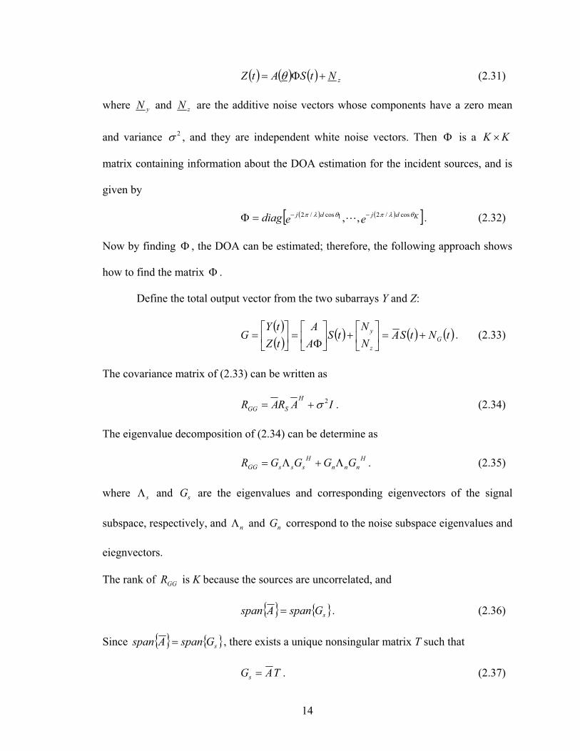
14
zNtSAtZ (2.31)
where yN and zN are the additive noise vectors whose components have a zero mean
and variance 2 , and they are independent white noise vectors. Then is a KK
matrix containing information about the DOA estimation for the incident sources, and is
given by
eediag Kdjdj cos/21cos/2 ,, . (2.32)
Now by finding , the DOA can be estimated; therefore, the following approach shows
how to find the matrix .
Define the total output vector from the two subarrays Y and Z:
tNtSAN
NtS
A
A
tZ
tYG G
z
y. (2.33)
The covariance matrix of (2.33) can be written as
IARARH
SGG
2 . (2.34)
The eigenvalue decomposition of (2.34) can be determine as
H
nnn
H
sssGG GGGGR . (2.35)
where s and sG are the eigenvalues and corresponding eigenvectors of the signal
subspace, respectively, and n and nG correspond to the noise subspace eigenvalues and
eiegnvectors.
The rank of GGR is K because the sources are uncorrelated, and
sGspanAspan . (2.36)
Since sGspanAspan , there exists a unique nonsingular matrix T such that
TAGs . (2.37)

15
The eigenvectors of estimate signal subspace sG can be partitioned into
TA
AT
G
GG
Z
Y
s (2.38)
where the dimension of ZY GG , is Km where M=2m.
The new matrix can be defined as Km 2
ZYYZs GGG . (2.39)
The rank of YZsG is K, which implies that there exists a unique matrix KKCF 2 of
rank K such that
ZYZZYYZY TFAATFFGFGFGG0 (2.40)
where F spans the null space of YZsG . Now a KK matrix can be defined as
1
ZY FF . (2.41)
Equation (2.40) can be written as
ATAT 1 . (2.42)
Assume A is full rank, which implies
1TT (2.43)
which can be rewritten as
TT 1 . (2.44)
According to equation (2.44), the eigenvalues of are equal to the diagonal
elements of , and the eigenvectors of are the columns of T. This is the main
relationship in the development of ESPRIT. There are many ways to estimate from
the array signal measurements [56-58]. The most popular one is TLS-ESPRIT [9, 56].
16
CHAPTER 3
CONJUGATE ESPRIT (C-SPRIT)
This chapter presents an algorithm to estimate the 1-D and 2-D DOA from
uncorrelated 1-D and 2-D signal sources, such as binary phase-shift keying (BPSK) and
M-array amplitude shift keying (MASK). The proposed algorithm can provide a more
precise DOA estimation and can detect more signals than the well-known classical
subspace methods, MUSIC and ESPRIT, for the 1-D and 2-D DOA. The complexity is
the same as that of ESPRIT, since the proposed algorithm uses the same array geometry
and subarray processing as ESPRIT. Also, both require the EVD or SVD. The main
differences between the proposed and ESPRIT algorithms are as follows: (1) in the
proposed algorithm, the number of overlapping array elements between the two subarrays
is equal to M, while in ESPRIT, the maximum number of overlapping elements is 1M ,
where M denotes the total number of array elements, and (2) the proposed algorithm
employs the conjugate of rotation matrix (CRM) , while ESPRIT uses with no
conjugate for the second subarray geometry.
3.1 Introduction
In the last two decades, considerable research efforts have been made to estimate
the parameters of the wavefronts arriving at the elements of an antenna array. Estimating
the direction of arrival angles from radio frequency signals has been of strong interest in
wireless communication systems such as radar, sonar, and mobile systems. The classical

17
subspace-methods, MUSIC [14] and ESPRIT [9], are included in the most popular
algorithms for the DOA estimation.
The MUSIC algorithm has substantial performance advantages. It is considerably
costly in terms of computation and storage for searching over parameter space. ESPRIT
dramatically reduces these computation and storage costs; however, ESPRIT does not
perform as well as MUSIC. Both MUSIC and ESPRIT display poor performance for joint
azimuth and elevation DOA estimation. Although many variations of MUSIC and
ESPRIT are available in the literature, existing joint-DOA estimation schemes with
reasonable complexities have not shown satisfactory performances. Moreover, the
extension scheme for a 2-D DOA estimation requires pair matching, which is considered
a critical issue in 2-D estimation in order to find the correct pair of azimuth and elevation
angles for multiple sources, whereas the proposed algorithm C-SPRIT does not require
any pair matching.
Presented here is an efficient algorithm that can estimate DOAs from the
uncorrelated (i.e., noncoherent) and one-dimensional signals such as BPSK and MASK.
Nameed C-SPRIT, it employs ESPRIT and the conjugate of the rotation matrix * for the
subarray processing 2. C-SPRIT employs information from observing all array element
outputs for the first and second subarray processing, without dividing the array elements
into several groups and without taking the average of covariance matrices, as the spatial
smoothing technique [59] does.

18
3.2 System Model
Consider a ULA composed of M elements and assume that K noncoherent and
narrow band one-dimensional signals are received at the ULA with different DOAs,
K,...,, 21 . The M×1 received signal vector can be written as
)()()()(1
tntsatX kk
K
k
(3.1)
where )(tsk represents the signal from the k-th sources with DOA equal to k, a( k),
which denotes the M×1 array response vector, and n(t) is the M×1 AWGN vector with
each component of mean zero and variance equal to 2. The array response vector can be
written as
KkzzzaTM
kkkk ,...,1,,...,,,1)( 12 (3.2)
where the superscript T stands for the transpose
kk
djz
cos2exp , (3.3)
is the wavelength, and d is the spacing between two successive antenna array
elements. The M×K array response matrix and K×1 signal vector can be written as
)(),...,(),()( 21 KaaaA (3.4)
and
T
K tstststS )(),...,(),()( 21 , (3.5)
respectively. The received signal vector can be rewritten as:
)()()()( tntSAtX . (3.6)

19
The following sections present the C-SPRIT algorithm, which can estimate either the
azimuth DOA k or the joint azimuth and elevation DOA ( k , k ), without the
requirements of pair matching.
3.3 Azimuth DOA Estimation with C-SPRIT
The C-SPRIT takes measurements from all the elements, denotes them as a
column vector (y1, y2,…, yM)T, and uses them for the subarray-1 processing. In fact, two
separate subarrays do not exist they are fully overlapped. Only the inputs to the subarray
processing 1 and 2 are differently ordered. Figure 3.1 shows the inputs to the subarray-1
and subarray-2 processing. The inputs to the subarray processing 1 are (y1, y2,…, yM) and
those for the subarray processing 2 are (y2*, y1,…, yM-1). This section offers an explanation
why the inputs to the subarray 2 should be in the form of (y2*, y1,…, yM-1). The proposed
C-SPRIT algorithm does not use any doublet concept as does the standard ESPRIT. Each
subarray processing in C-SPRIT uses the maximum number of array elements equal to M,
whereas each subarray processing in ESPRIT can have only M/2 elements for the doublet
case or M-1 at most, for the maximum overlap case. This is the major rationale for why
CSPRIT can have better signal-to-noise power ratio (SNR) or a better performance than
ESPRIT.

20
)1(subarray
)2(subarray
1y
2y1y 1My2y
My2y 3y
Figure 3.1. The inputs to subarray 1 and 2 processing, (y1, …, yM) and (y2*, y1 …, yM),
respectively, for the proposed C-SPRIT algorithm, where y1, …, yM are the received
signals at element 1,…, M, of an array, respectively.
The first element in the array is treated as the reference with respect to the other
elements, as shown in Figure 3.1. In this case, the M×1 input vector to subarray-1 can be
written as
)()()()( 11 tntSAtY (3.7)
22
2
2
1
22
2
2
1
21
111
)(
M
K
MM
K
K
zzz
zzz
zzz
AA (3.8)
T
M tytytytY )](),...,(),([)( 211 (3.9)
T
M tntntntn )](),...,(),([)( 211 (3.10)
where A( ) is the array response matrix with dimensions M×K (not m×K used for the
conventional ESPRIT, m M-1), )(tS is the narrowband signal vector with dimension
K×1, and n1(t) is the M×1 AWGN vector whose component has a zero mean and
variance equal to 2 .
The input vector to the subarray-2 processing is written as

21
T
MyyytY ],...,,[)( 1122 . (3.11)
This input vector can be rewritten in terms of )(A , )(tS , and as
)()()()( 2
1
1
2
2
1
1
1
*
2
1
*
2 tntSA
nzs
nzs
ns
nzs
tY
M
K
k
M
kk
K
k
kk
K
k
k
K
k
kk
(3.12)
for the one-dimensional signals such as BPSK and MASK where sk=sk*
),...,,( 21 Kzzzdiag (3.13)
T
M tntntntn )](),...,(),([)( 1122 . (3.14)
These two observation vectors, Y1 and Y2, are employed in this chapter. Hence, the total
output vector )(tZ can be written as
)()()(
)()(
2
1tntBS
tY
tYtZ (3.15)
where
A
AB (3.16)
)(
)()(
2
1
tn
tntn (3.17)
where B is a 2M×K matrix, and both )(tZ and n(t) are 12M vectors. Forming the
2M×2M covariance matrix Z(t) from the measurement data,
IBBRR H
SZZ
2 (3.18)

22
where the superscript H donates the Hermitian operator. The K×K signal covariance
matrix is ])()([ H
S tStSER . The signals are uncorrelated, and the 2M-K smallest
eigenvalues of RZZ are equal to 2. The K eigenvectors corresponding to the K-largest
eigenvalues can be written in an 2M×K matrix as
],...,,[ 21 KS eeeF . (3.19)
The range space of FS is equal to that of B, i.e., )()( BFS . Thus, a nonsingular
matrix T exist such that BTFS . By decomposing SF into two M×K matrices, F0 and
F1,
TA
AT
F
FFS
1
0. (3.20)
Using equation (3.20) and following the procedure in [9] can be written as:
1TT . (3.21)
where the eigenvalues of matrix are equal to the diagonal elements of , and the
columns of T are the eigenvectors of . So finding leads to finding . The value
of can be found by applying the straightforward approach least-squares (LS) [60, 61].
However, under noisy measurements in practical situations, least-squares may be
inappropriate. Instead, is often solved by using the total-least-squares (TLS) method
[62-65]. In the algorithms in this chapter, the same TLS method is applied to find the
DOAs by using the following steps:
Step 1 - Obtain the estimate of ZZR from the measurements.
Step 2 - Apply eigenvalue decomposition on ZZR , i.e.,
H
ZZZZ FFR (3.22)

23
where MZZ diag 221 ,...,, and MeeeF 221 ,...,, .
Step 3 - Use the multiplicity k of the smallest eigenvalue to estimate the number
of signals as
kMK 2ˆ . (3.23)
The k would be M, if K=M is a special case.
Step 4 - Estimate the signal subspace SF̂ using the eigenvectors corresponding to
the largest K eigenvalues, and decompose SF̂ into two (M×K) sub-matrices 0F̂ and 1F̂ ,
where
1
0
ˆ
ˆˆ
F
FFS . (3.24)
Step 5 - Apply the eigenvalue decomposition on the matrix formed as
H
GH
H
FFFFF
FG 10
1
0 ˆˆˆ
ˆ. (3.25)
Partition F into KK ˆˆ sub-matrices
2221
1211
FF
FFF . (3.26)
Step 6 - Calculate the eigenvalues k of , where 1
2212 FF . Then, estimate
the k-th diagonal element *ˆk of *ˆ as
kkˆ , k 1, 2, ..., K̂ . (3.27)
Step 7 - Estimate the azimuth DOA using equation (3.3) and equation (3.13) as
/2
)ˆarg(cosˆ 1
dk
k . (3.28)

24
3.4 Joint Azimuth and Elevation 2-D DOA Estimations with C-SPRIT
The same TLS method can apply to estimate the elevation and azimuth 2-D DOA
jointly using C-SPRIT. Two uniform linear orthogonal arrays are used in the x-z plane, as
shown in Figure 3.2. The antenna couplings between the two orthogonal arrays are
negligible for the simplicity. This assumption is valid if the first element in the z-axis is
placed far enough from those in the x-axis, e.g., ten wavelengths from the origin. The
process in this TLS method is a follows:
1. Collect data from the array elements in the z-axis, and apply the proposed C-
SPRIT algorithm.
2. Apply steps 2 through 7 to estimate the elevation angle kˆ , and replace the
estimation kˆ in equation (3.28) with k
ˆ . Then, the estimation of elevation DOA *ˆk can
be written as
/2
)ˆarg(cosˆ 1
dk
k . (3.29)
3. To estimate the azimuth angle, collect data from the array elements in the x-
axis and apply the proposed C-SPRIT algorithm. In this case, the array response vector is
similar to the one in equation (3.2). Here kz is a function of both elevation DOA k and
azimuth DOA k , and zk can be written as
kkk
djz
ˆsinˆcos2exp . (3.30)
Thus, the azimuth DOA estimation kˆ can be written as

25
/)ˆsin2(
))arg(cosˆ 1
k
kk
d (3.31)
where kˆ was obtained from equation (3.29). Equations (3.29) through (3.31) can be
applied in the similar way for the other algorithms such as ESPRIT and MUSIC.
k
k
1
1
2
2
3
3
4
4
5
5
8N
x
z
y
d
d
Kk ,...,1)(tsk
6
7
7
6
8M
Figure 3.2. Two uniform linear orthogonal arrays used for joint elevation and azimuth
DOA estimations.
The basic differences between the proposed C-SPRIT and ESPRIT algorithms are
shown in Table 3.1.

26
Table 3.1 Basic differences between ESPRIT algorithm and proposed C-SPRIT
algorithm
Property ESPRIT Algorithm C-SPRIT Algorithm
Phase shift-delay matrix
Number of elements in each
subarray1M M
Maximum number of sources 1M M
Pair matching for ( k , k ) required not required
Modulation BPSK, QPSK, MASK BPSK, MASK
3.5 Simulation Results
The assumption is made that K=3, 4, or 6 signals are from BPSK sources for
simulation. A uniform linear array consisting of M=6 or eight elements separated by
distance equal to a half wavelength of the incoming signals is employed. The number of
data samples per trial at each element output is N=200 and the number of total
independent trials used was 2500.
A. Simulation 1
Figures 3.3, 3.4, and 3.5, show the histograms of the azimuth DOA estimation for
K = 3 sources of DOA at [82º, 90º, and 98º], SNR = [2, 2, 2] dB, and M=6 elements. It
becomes clear in Figure 3.3 that the proposed algorithm gives the most accurate DOA
estimations most of the time, and all three peaks are observed at around 82º, 90º, and 98º,
whereas in Figures 3.4 and 3.5, only two peaks and the signal of DOA equal to 90º is
missing. The ESPRIT algorithm with maximum overlapping and no overlapping,

27
respectively often do not give accurate estimations. The standard ESPRIT with no
overlapping gives worse estimations than ESPRIT with maximum overlapping.
Figure 3.3. Histogram of DOA estimations for K=3 sources of DOA at [82º, 90º, 98º],
SNR= [2, 2, 2] dB, and M = 6 elements for proposed algorithm C-SPRIT.
Figure 3.4. Histogram of DOA estimations for K=3 sources of DOA at [82º, 90º, 98º],
SNR= [2, 2, 2] dB, and M = 6 elements for ESPRIT maximum overlapping.

28
Figure 3.5. Histogram of DOA estimations for K=3 sources of DOA at [82º, 90º, 98º],
SNR=[2, 2, 2] dB, and M = 6 elements for ESPRIT with no overlapping.
B. Simulation 2
For this simulation, Table 3.2 lists the averages and variances of the azimuth
DOA estimations using the two ESPRITs and our C-SPRIT algorithm. We observe in
Table 3.2 that our proposed C-SPRIT algorithm provides the most accurate estimation of
DOAs, compared to ESPRIT. For example the averages of the DOA estimations with the
proposed C-SPRIT are [82º, 90.01º, 97.99º], and the variances are [1.55, 3.53, 1.51],
while the averages of the DOA estimations with the ESPRIT of maximum overlapping
elements are [81.57º, 89.9º, 98.39º], and the variances are [9.46, 12.76, 9.12],
respectively. The averages of the DOA estimations with the ESPRIT algorithm of no
overlapping are [68.86º, 89.91º, 110.4º], and the variances are [597, 55.57, 559],
respectively.

29
Table 3.2 Means and variances of DOA estimation at SNR=2 dB: (1) proposed C-SPRIT,
(2) ESPRIT with maximum overlapping, and (3) ESPRIT with no overlapping K=3 and
M=6.
C. Simulation 3
This simulation presents the simulation results for the case of K=M=6, which is
an example of the number of signals equal to the number of antenna array elements.
Figure 3.6 shows sharp histograms for the azimuth DOA estimations using the proposed
C-SPRIT. Six signals are present with DOAs at 20º, 40º, 60º, 80º, 100º, and 120º and a
SNR of 15 dB. The number of antenna array elements is also equal to six. The means of
estimated angles [19.975º, 39.994º, 59.999º, 80.003º, 99.998º, and 119.996º] are very
close to the actual values, and variances are small as [0.268, 0.070, 0.020, 0.011, 0.010,
and 0.014]. Figure 3.7 shows the corresponding results for ESPRIT in the maximum
overlapping case. Five sources are detected with averages of 27.85º, 55.23º, 77.88º,
98.851º, and 119.2º and variances of 0.135, 0.217, 0.264, 0.217, and 0.123, respectively.
One signal is missing and many estimated values are not close to the actual values.
Proposed
Algorithm
ESPRIT Algorithm
(Max Overlapping)
ESPRIT Algorithm
(No Overlapping)
Incident
Azimuth
DOA Angle
(degrees) Mean Variance Mean Variance Mean Variance
82 82.006 1.550 81.574 9.460 68.860 597.113
90 90.013 3.534 89.900 12.760 89.912 55.571
98 97.999 1.512 98.391 9.120 110.40 559.214

30
Figure 3.6. Histogram of DOA estimations K=6 sources of DOA at [20º, 40º, 60º, 80º,
100º, 120º], SNR = [15, 15, 15, 15, 15, 15] dB, and M=6 elements for proposed
algorithm C-SPRIT
Figure 3.7. Histogram of DOA estimations K=6 sources of DOA at [20º, 40º, 60º, 80º,
100º, 120º], SNR = [15, 15, 15, 15, 15, 15] dB, and M=6 elements for ESPRIT with
maximum overlapping, where the highest M-1=5 eigenvalues were used.
31
D. Simulation 4
This simulation considers the joint azimuth and elevation DOA estimations. K=4
uncorrelated sources are received with elevation and azimuth DOAs at (40º, 80º), (50º,
90º), (60º, 100º), and (70º, 110º), respectively, signal-to-noise-ratio (SNR) of 3 dB, and
M=8 elements.
Figures 3.8 through 3.13 show the histograms of the joint elevation and azimuth
angle DOA estimations by using the proposed C-ESPRIT, ESPRIT with maximum
overlapping and ESPRIT with no overlapping. It becomes clear in Figures 3.8 and 3.11
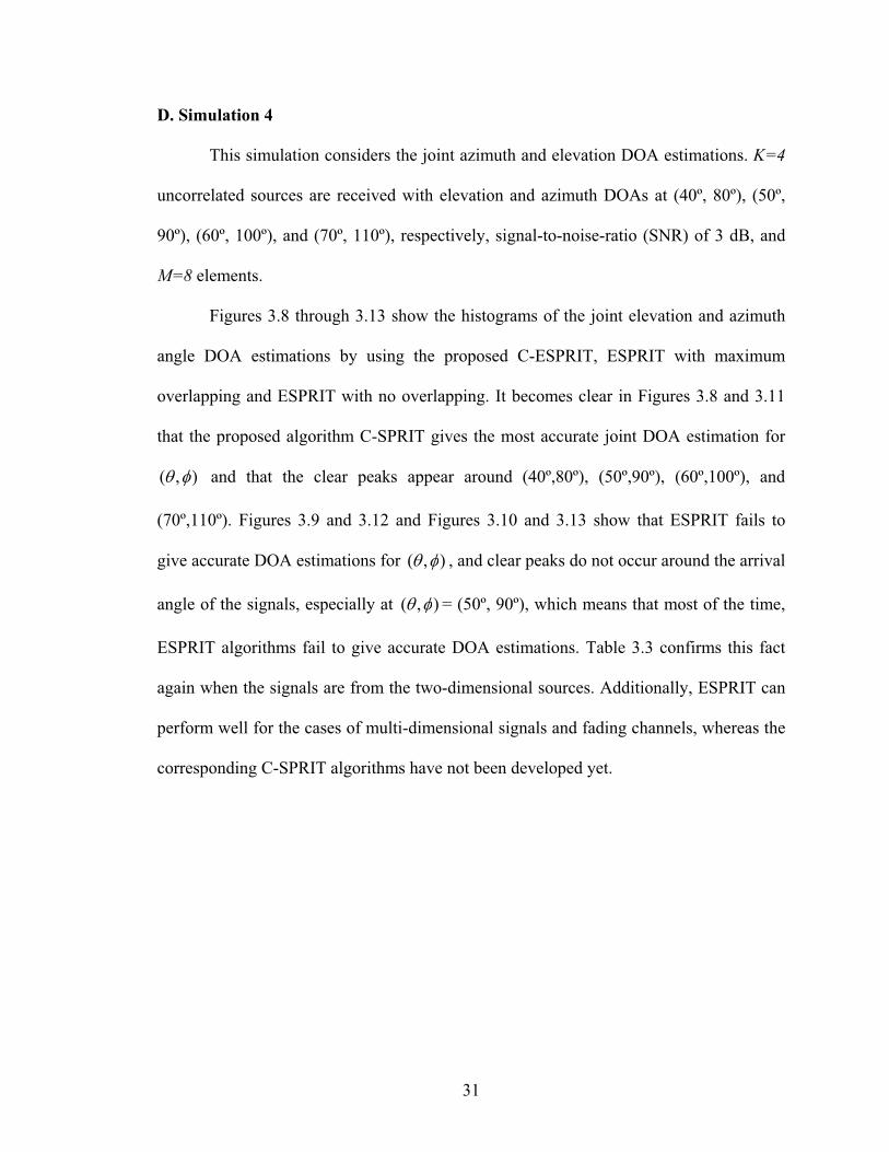
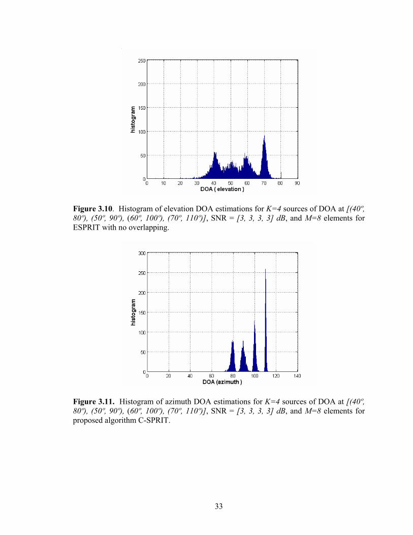
that the proposed algorithm C-SPRIT gives the most accurate joint DOA estimation for
),( and that the clear peaks appear around (40º,80º), (50º,90º), (60º,100º), and
(70º,110º). Figures 3.9 and 3.12 and Figures 3.10 and 3.13 show that ESPRIT fails to
give accurate DOA estimations for ),( , and clear peaks do not occur around the arrival
angle of the signals, especially at ),( = (50º, 90º), which means that most of the time,
ESPRIT algorithms fail to give accurate DOA estimations. Table 3.3 confirms this fact
again when the signals are from the two-dimensional sources. Additionally, ESPRIT can
perform well for the cases of multi-dimensional signals and fading channels, whereas the
corresponding C-SPRIT algorithms have not been developed yet.

32
Figure 3.8. Histogram of elevation DOA estimations for K=4 sources of DOA at [(40º,
80º), (50º, 90º), (60º, 100º), (70º, 110º)], SNR = [3, 3, 3, 3] dB, and M=8 elements for
proposed algorithm C-SPRIT.
Figure 3.9. Histogram of elevation DOA estimations for K=4 sources of DOA at [(40º,
80º), (50º, 90º), (60º, 100º), (70º, 110º)], SNR = [3, 3, 3, 3] dB, and M=8 elements for
ESPRIT with maximum overlapping.
33
Figure 3.10. Histogram of elevation DOA estimations for K=4 sources of DOA at [(40º,
80º), (50º, 90º), (60º, 100º), (70º, 110º)], SNR = [3, 3, 3, 3] dB, and M=8 elements for
ESPRIT with no overlapping.
Figure 3.11. Histogram of azimuth DOA estimations for K=4 sources of DOA at [(40º,
80º), (50º, 90º), (60º, 100º), (70º, 110º)], SNR = [3, 3, 3, 3] dB, and M=8 elements for
proposed algorithm C-SPRIT.

34
Figure 3.12. Histogram of azimuth DOA estimations for K=4 sources of DOA at [(40º,
80º), (50º, 90º), (60º, 100º), (70º, 110º)], SNR = [3, 3, 3, 3] dB, and M=8 elements for
ESPRIT with maximum overlapping
Figure 3.13. Histogram of azimuth DOA estimations for K=4 sources of DOA at [(40º,
80º), (50º, 90º), (60º, 100º), (70º, 110º)], SNR = [3, 3, 3, 3] dB, and M=8 elements for
ESPRIT with no overlapping.

35
Table 3.3 Means and variances of joint azimuth and elevation DOA estimation at SNR =
3dB: (1) proposed C-SPRIT, (2) ESPRIT with maximum overlapping, and (3) ESPRIT
with no overlapping. K=4 and M=8.
Proposed Algorithm ESPRIT Algorithm
(Max Overlapping)
ESPRIT Algorithm
(No Overlapping)
Estimation of
Azimuth ( ˆ )
and Elevation
( ˆ )Mean Variance Mean Variance Mean Variance
1ˆ 39.3229 1.3120 39.9951 5.4750 39.5038 11.5758
1ˆ 79.0863 2.2165 79.9498 6.0955 79.0871 42.3163
2ˆ 49.4146 2.5416 50.1445 9.6829 49.8604 12.5949
2ˆ 89.4138 3.0517 90.2387 9.9852 90.2335 13.4437
3ˆ 60.1718 1.2428 59.9744 5.7786 60.0981 7.7467
3ˆ 99.9756 0.9561 100.0811 4.9079 100.2189 7.1818
4ˆ 70.2138 0.2223 69.9567 1.1795 70.3171 19.8971
4ˆ 110.0944 0.2380 109.9120 1.0129 110.2929 13.8173
3.6 Summary
This chapter presented the C-SPRIT algorithm to find the direction of arrival
angles for noncoherent, narrowband, and 1-D and 2-D DOA signals such as BPSK and
MASK. Analytically, the proposed algorithm can employ the conventional ESPRIT
signal processing with insignificant changes and negligible additional complexities. The
C-SPRIT uses only one array for two subarray processings, whereas ESPRIT employs
two subarrays for two subarray processings. Simulation results show that the proposed C-
SPRIT yields the highest resolution, especially at a low SNR and small angle separations
between the signals. In addition, the proposed C-SPRIT can identify the DOAs, even if

36
the number of sources is equal to the number of antenna array elements, whereas MUSIC
and ESPRIT fail. Furthermore, compared with ESPRIT, the proposed C-SPRIT algorithm
provides exemplary performance, even for joint azimuth and elevation DOA estimations.
37
CHAPTER 4
2-D DOA ESTIMATION BASED ON NON-EIGENANALYSIS
Recently, a Virtual Estimation of Signal Parameters Rotational Invariance
Techniques (V-ESPRIT) has been proposed for the 2-dimensional estimation, i.e., the
azimuth and elevation angles from the sources. The V-ESPRIT has computational cost,
which is close to that of the 1-D ESPRIT algorithm for the 2-D sources. The V-ESPRIT
requires either the eigenvalue decomposition (EVD) of the cross-correlation matrix or the
singularvalue decomposition (SVD) of the received data matrix as the 1-D ESPRIT.
Thus, the computational load of the V-ESPRIT is in o(n3) for an n×n matrix.
This chapter employs the propagator method, which does not require any EVD or
SVD to the V-ESPRIT. The proposed PMV-ESPRIT reduces the computational
complexity further for the 2-D sources when compared to the V-ESPRIT. The
performance of the PMV-ESPRIT with the V-ESPRIT and the PM of the doublet
configurations [24] were compared. The PMV-ESPRIT showed several advantages over
the PM [24]: (1) a lower computational complexity that is close to 1-D estimation, (2) no
pair matching between azimuth and elevation angles from the 2-D estimation for different
sources, as in the case with PM, and (3) less information data from the antenna array to
find the azimuth and elevation angles.
4.1 Introduction
The most popular techniques for DOA estimation are the MUSIC and ESPRIT
algorithms [9, 14]. These algorithms employ either eigenvalue decomposition of the cross

38
spectral matrix of the received signal, or the singularvalue decomposition of the received
data matrix. Using these techniques to estimating the DOAs has shown significant
improvement. However, their computational complexities are costly, especially when the
number of sources is large and the 2-dimensional DOA estimations, such as the azimuth
and elevation angles, are desirable. The computational complexity of ESPRIT can be in
the order of N3+2N
2L, that is LNNO 23 2 multiplications with an N-element array,
with L snapshots.
The aim of this proposed method is to reduce the computational load up to
NLKO 2 multiplications for on-line processing and minimal storage, where K is the
number of sources. To achieve this goal, the PM [33, 24] is used to estimate the 2-D
DOAs of the incident signals without using EVD of the CSM and SVD of the RDM. The
PM is a linear operation based on the partition of the steering vectors. The PM estimates
the DOAs from the sources by applying the least squares method to the received data
matrix or the cross-spectral matrix. Thus, the PM only has a NLKO 2 computational
load for the 2-D DOA estimations.
A disadvantage of the PM [24] of doublet configuration is the pair matching
between the estimated azimuth angle i from the source i, and the estimated elevation
angle k from the source k because the azimuth and elevation DOA estimations with the
PM in this case are not in order. In addition, using triplet configuration [66] can convert
the 2-D estimation problem to 1-D, whereas PM [24] cannot do this. The PM using
doublets configuration requires more information data to estimate , , and the number
of multiplications involved to calculate the propagator is in LKNO 3 , where N is the
number of elements in each subarray of the doublet configuration. However, the proposed

39
method PMV-ESPRIT has only NLKO 2 multiplications, where N is the number of
elements in each subarray of the triplets and NN . For comparison, it is assumed that
the total number of elements of the PMV-ESPRIT is the same as that of the PM [24].
Furthermore, this proposed method is used to avoid the pair matching problem in
the PM by employing the antenna array configuration of the Virtual ESPRIT algorithm
[66]. The V-ESPRIT uses the triplet antenna array configuration instead of the doublet
which has been used in the ESPRIT [9], [24]. This triplet configuration can convert a 2-D
DOA estimation problem into a 1-D. Unfortunately, the V-ESPRIT employs the
conventional ESPRIT algorithm. Therefore, the computational complexity of the V-
ESPRIT is on the order of LNNO 23 2 . The proposed method applies the PM to the V-
ESPRIT so that the overall computational load can be reduced from LNNO 23 2 to
NLKO 2 . In addition, the 2-D DOA estimation and pair matching burden required by
the PM can be removed in the proposed method.
4.2 Proposed Algorithm: PMV-ESPRIT using Triplets Configurations
Consider a uniform array that consists of N triplets, each containing three
elements [66] as shown in Figure 4.1. Suppose that there are K uncorrelated narrowband
sources, where the k -th source has an elevation angle k and an azimuth angle k .

40
xd
yd
X
Y
1,0Z 2,0Z NZ ,0
1,1Z
1,2Z
2,1Z
2,2Z
NZ ,1
NZ ,2
triplet triplet triplet1 2 N
Figure. 4.1. Uniform elements array composed of triplets.
The elements in Figure 4.1 can be divided into three sub-arrays of no shared
elements. The received signal vectors at the 1st, 2
nd, and 3
rd sub-array are denoted by N×1
vector, respectively,
T
NZZZZ 002010 ,, (4.1)
T
NZZZZ 112111 ,, (4.2)
T
NZZZZ 222212 ,, (4.3)
where the superscript T denotes the transpose. These received vectors can be rewritten as
00 nASZ (4.4)
111 nSAZ (4.5)
222 nSAZ (4.6)

41
where A is the N×K matrix of the steering vectors a( k), k=1, …, K, S is a K×1 signal
vector of K source signals, and 10 , nn and 2n are the N×1 additive white Gaussian noise
(AWGN) vectors whose elements have mean zero and variance 2 . The 1 and 2 are
K×K diagonal matrices containing information about the elevation and azimuth angles,
which can be written as
KyKxyxdd
jdd
jdiagcos2cos2
expcos2cos2
exp11
1 (4.7)
KyKxyxdd
jdd
jdiagcos2cos2
expcos2cos2
exp11
2 (4.8)
where , k, k, dx, and dy are the wavelength, the elevation angle, the azimuth angle,
and the x and y coordinates of the two sensors in the 1st triplet, respectively. Equations
(4.7) and (4.8) have both azimuth and elevation angle information together in their
exponents. One way to separate them is to add 1Z and 2Z as
2/21 ZZZ . (4.9)
Then
nSAZ (4.10)
where 2/)( 21 nnn has the same variance 2 as ni, and i=0, 1, and 2 . The is a
K×K diagonal matrix written as
KxKyxy dj
ddj
ddiag
cos2exp
cos2cos,,
cos2exp
cos2cos2 11
.
(4.11)
42
The azimuth angle information for K sources is in the amplitude components, and
the corresponding elevation angle information is in the phase components of the diagonal
elements in equation (4.11). In the proposed method PMV-ESPRIT, is found by using
the propagator method [24] whose computational load is proportional to NLKO 2 . Then
the 2-D DOA estimations can be easily made from the diagonal elements of by
observing their amplitude and phase separately. This does not require any pair matching
between the source azimuth and elevation angles.
A definition of the propagator method [33] is used for the proposed method. It is
based on the partition of the array response vector as follows
TTT AAA 21 (4.12)
where 1A and 2A are sub-matrices with dimension KK and KKN , respectively.
The propagator is then applied to the observation output vectors Z0 and
2/21 ZZZ in equations (4.4) and (4.10), respectively. Let D denote
TTT AAD . (4.13)
After partitioning D in a similar way, it can be written as
TTT DAD 11 (4.14)
where
TTTT AAAD 2121 . (4.15)
Under the hypothesis that 1A is a non-singular matrix (which is common for all the
subspace-based methods with N 2K), the propagator P is a unique linear operator,
which can be written as
11 DAPH (4.16)

43
where H is the Hermitian operator, i.e., conjugate and transpose.
Let z(t) denote a 2N×1 snapshot data vector written as
TTT tZtZtz 0 , t=1,…, L. (4.17)
Also let X denote the 2N×L data matrix consisting of L snapshots as
.)(...),2(),1( LzzzX (4.18)
Then, the 2N×2N cross spectral matrix can be written as
L
t
HH tztzL
XXL
R1
)()(11ˆ . (4.19)
The partitions of the data matrix X and cross-spectral matrix R̂ can be written as
2
1
X
XX (4.20)
and
JFR̂ (4.21)
where 1X and 2X are sub-matrices with dimension LK and LKN )2( ,
respectively, and F and J are sub-matrices with dimension KN2 and
KNN 22 , respectively.
Let dataP̂ and csmP̂ denote the K×(2N-K) and K×(2N-K) propagator estimate
matrix based on the data matrix X and cross-spectral matrix R̂ , respectively. The
optimum propagator estimate matrix can be found by applying the least-squares method
on equations (4.20) and (4.21) as
HH
data XXXXP 21
1
11ˆ (4.22)
JFFFP HH
csm
1ˆ . (4.23)
44
csmP̂ (or dataP̂ ) can be partitioned as
TTTTH
csm PPPP 321ˆˆˆ (4.24)
where the dimension 1P̂ , 2P̂ , and 3P̂ are identical with the dimension 2A , 1A , and 2A ,
respectively.
According to equation (4.16), and using equations (4.15) and (4.24), we can write
the equations as
211ˆ AAP (4.25)
112ˆ AAP (4.26)
213ˆ AAP . (4.27)
Equations (4.25) and (4.27) can be used to find by solving the eigenvalues of 2P̂ from
equation (4.26) as
22
#
13ˆˆ AAPP (4.28)
where # donates the pseudoinverse. This means that the estimation of the diagonal
elements of matrix can be obtained by finding the K eigenvalues of #
13ˆˆ PP . The
dimension of #
13ˆˆ PP is KK , which is much smaller than 2N×2N of R̂ , which is used for
EVD in ESPRIT or V-ESPRIT. Then, using the eigen-value factorization, we can write
#
13ˆˆ PP as
1
11
#
13ˆˆ VVPP (4.29)
where 1V represents the eigenvector matrix, and is the diagonal matrix of the
eigenvalues of #
13ˆˆ PP . Then, from equation (4.11), the azimuth and elevation angles for
each source can easily found as

45
2
cos2
cosˆ ,11 kk
y
k
amplitude
d (4.30)
kk
x
k phased
,
1
2cosˆ . (4.31)
Therefore, the proposed PMV-ESPRIT algorithm takes only NLKO 2 major
computational multiplications.
4.3 Simulation Results
The simulation results of the proposed method PMV-ESPRIT were compared
with the V-ESPRIT and the PM of doublet configuration for the 2-D azimuth and
elevation DOA estimations. Three uniform antenna arrays were employed for the triplet
configuration, as shown in Figure 4.1, which consists of 15 elements. The assumption is
made that 2K uncorrelated sources with direction , = 60,30 and 30,60 ,
4/yd , and 2/xd . The simulation results are based on the 200L number of
snapshots per trial at each element and 1000 total independent trials.
A. Simulation 1
From this simulation, Figures 4.2 and 4.3 show the plot of the standard deviation
of the DOA estimation errors in degree versus SNR values for Source 1 with direction
, = 60,30 . These figures show that the performance of the proposed algorithm
PMV-ESPRIT is the same as that of the V-ESPRIT algorithm for the wide range of SNRs
but is slightly worse than that of the PM with doublet configuration whose computational

46
complexity is higher than the proposed PMV-ESPRIT. Also the computational
complexity of the proposed PMV-ESPRIT is reduced significantly by using PM from
LNNO 23 2 in V-ESPRIT to NLKO 2 .
Figure 4.2. Standard deviation versus SNR for elevation angle 30 degrees from Source 1
for the proposed PMV-ESPRIT, V-ESPRIT algorithm, and the PM with doublet.
Figure 4.3. Standard deviation versus SNR for azimuth angle 60 degrees from Source 1
for the proposed PMV-ESPRIT, V-ESPRIT algorithm, and the PM with doublet

47
B. Simulation 2
From this simulation, Figures 4.4 and 4.5 show the plot of the standard deviation
of the DOA estimation errors in degrees versus SNR values for Source 2 with direction
, = ( 30,60 ) . These figures show that the performance for Source 2 is almost the
same as for Source 1.
Figure 4.4. Standard deviation versus SNR for elevation angle 60 degrees from Source
2 for the proposed PMV-ESPRIT, V-ESPRIT algorithm, and propagator method with
doublet.

48
Figure 4.5. Standard deviation versus SNR for azimuth angle 60 degrees from Source 2
for the proposed PMV-ESPRIT, V-ESPRIT algorithm, and propagator method with
doublet.
4.4 Summary
This chapter proposes that PMV-ESPRIT does not use any EVD and SVD,
whereas V-ESPRIT does. Therefore, the proposed PMV-ESPRIT can reduce the
complexity LNNO 23 2 of the V-ESPRIT to NLKO 2 and also does not need the
pair matching between the azimuth and elevation angles as in the PM with doublet
configuration. Furthermore, the performance of the proposed PMV-ESPRIT is the same
as that of the V-ESPRIT although slightly worse than the PM with doublet configuration
whose computational complexity is higher than the proposed one. Hence, the PMV-
ESPIRIT will be more appropriate than the V-ESPIRIT or the PM with doublet
configuration for real-time implementation.

49
CHAPTER 5
L-SHAPE 2-D ARRIVAL ANGLE ESTIMATION WITH PROPAGATOR
METHOD
It is known that computational loads of the propagator method can be
significantly smaller, e.g., one or two orders of magnitude, than those of MUSIC and
ESPRIT because the PM does not require any eigenvalue decomposition of the cross-
correlation matrix and singularvalue decomposition of the received data.
However, the PM of the parallel shape array has non-negligible drawbacks: (1)
requirement of pair matching between the 2-D azimuth and elevation angle estimation,
which is an exhaustive search, and (2) estimation failure problems when elevation angles
are between 70 and 90 degrees. The purpose of this chapter is to show a way to remove
these problems in the PM without additional computational loads. The proposed method
uses one or two L-shape arrays because the parallel shape used in the PM may cause the
aforementioned problems. Simulation results verify that the PM with one or two L-shape
configurations can remove these problems and improve the performance of the PM
significantly, e.g., almost 5 dB in the signal-to-noise-ratio for the parameters used in this
chapter.
5.1 Introduction
Marcos and co-workers [31-34] suggested the so-called “propagator” method for
array signal processing without any eigenvalue decomposition. However, the PM of the
parallel-shape array in [24] requires pair matching between the 2-D azimuth and
elevation angle estimation , and can have an estimation failure problem when

50
elevation angles are between 70 and 90 degrees. The elevation angle in typical mobile
communications is in this range. Thus, the application of the PM of the parallel-shape
array to mobile communications should be reconsidered. The parallel-shape array used in
the PM [24] may cause the aforesaid problems.
The idea of using L-shaped arrays is not new, e.g., [25]. But the L-shape array in
this chapter is different from that in [25]. In the proposed method, the elements are placed
on the x-z or y-z axes whereas the elements in [25] are on the x-y axis. In addition, the L-
shape in [25, equation (10)] uses the same DOA estimation equations as the ones in [24,
equation (14)] and [25, equation (18)]. Therefore, the L-shape in [25] has the same pair
matching and failure problems as in [24, 26].
The purpose of this chapter is to show how to remove these problems in the PM
without additional computational loads. This chapter uses a configuration of one or two
L-shape arrays, which allow no pair matching between the azimuth angle estimate i for
source i and the elevation angle estimate k for source k. In addition, using an L-shape
array shows no elevation angle estimation failure, even if the elevation angle is between
70 and 90 degrees. Furthermore, the one L-shape array in the x-z plane shows several
other advantages over the parallel-shape array but has a failure problem similar to the one
in [24] when the azimuth angle is between 0 and 20 degrees. However, with the proposed
two L-shape arrays in the x-z and y-z planes, the failure problem can be completely
removed and the RMSE significantly reduced.

51
5.2 Proposed PM with One L-Shape Array
Figure 5.1(a) shows the one L-shape array configuration, which uses the x-z plane
instead of the x-y plane used in [25]. Each linear array consists of 1N elements. The
element placed at the origin is common for referencing purpose. Let X and Y be the two
subarrays of the linear array in the z axis, and let Z and W be the two sub-arrays of the
linear array in the x axis. Each sub-array consists of N-1 elements. Suppose that there are
K narrowband sources, where the k -th source has an elevation angle k and an azimuth
angle k , k=1, …, K.
N
subarray
X
Y
subarray
.
..
.
.
.
x
y
z
N
1
2
1N
1N
2subarray
subarray W
Z
k
k
)(tSk,1k .. ., K
Figure 5.1(a). Proposed one L-shape array configuration used for the joint elevation and
azimuth , DOA estimation.
Let the (N-1)×1 signal vectors received at the X and Y subarray be
T
N txtxtxtX )](),...,(),([)( 121, T
N tytytytY )](),...,(),([)( 32, respectively, where superscript T
denotes the transpose. These received vectors can be rewritten as

52
)()()()( tntSAtX x (5.1)
)()()()( 1 tntSAtY y (5.2)
where
)(),...,(),()( 21 KaaaA (5.3)
KkqqqaTN
kkkk ,...,1,,...,,,1)( 22 (5.4)
kk
djq
cos2exp (5.5)
and S is a K×1 signal vector for the K source signals, xn and yn are the (N-1)×1
additive white Gaussian noise vectors whose elements have a mean of zero and variance
2 . The largest factor in equation (5.4) should be (N-2) because the total number of the
elements in the z-axis is N-1 including the reference one at the origin. Two maximally
overlapping subarrays are considered in the z-axis array. Therefore, each subarray can
have maximum (N-1) elements. The matrix 1 in equation (5.2) is a K×K diagonal
matrix containing information about the elevation angle k , which can be written as
),...,,( 211 Kqqqdiag . (5.6)
We find 1 by using the propagator method [33, 24] whose computational load is
proportional to LKNO )1(2 . It is based on the partition of the array response vector as
TTT AAA 21 (5.7)
where 1A and 2A are sub-matrices with dimension KK and KKN 1 ,
respectively. The propagator can be applied on the observation output vectors X and Y
in equations (5.1) and (5.2), respectively. Let C be denoted by

53
TTT AAC 1 . (5.8)
After partitioning C in a similar way, it can be written as
TTT CAC 11 (5.9)
where
TTTT AAAC 121121 . (5.10)
Under the hypothesis that 1A is a non-singular matrix (which is common for all the
subspace-based methods with (N-1) 2K), the propagator P is a unique linear operator,
which can be written as
11 CAP H (5.11)
where H is the Hermitian operator, i.e., conjugate and transpose.
Let tr denote a 2(N-1) ×1 snapshot data vector written as
TTT tYtXtr )()()( , t=1,…, L. (5.12)
Also let F denote the (2(N-1) ×L) data matrix consisting of L snapshots as
)(),2(),1( LrrrF . (5.13)
Then, the 2(N-1)×2(N-1) cross-spectral matrix can be written as
HFFL
R1ˆ . (5.14)
The partitions of the data matrix F and cross spectral matrix R̂ can be written as
2
1
F
FF (5.15)
and
JER̂ (5.16)

54
where ( 1F , 2F ) are sub-matrices with dimensions LK and LKN ))1(2( ,
respectively, and ( E , J ) are sub-matrices with dimensions KN )1(2 and
KNN )12()1(2 , respectively.
Let dataP̂ and csmP̂ denote the K×(2(N-1)-K) and K×(2(N-1)-K) propagator
estimate matrix based on the data matrix F and cross spectral matrix R̂ , respectively.
The optimum propagator estimate matrix can be found by applying the least square
method on equations (5.15) and (5.16) as
HH
data FFFFP 21
1
11ˆ (5.17)
JEEEP HH
csm
1ˆ . (5.18)
csmP̂ (or dataP̂ ) can be partitioned as
TTTTHcsm PPPP 321
ˆˆˆ (5.19)
where the dimensions of 1P̂ , 2P̂ , and 3P̂ are identical with the dimensions of 2A , 11A ,
and 12A , respectively.
According to equation (5.11), and using equations (5.10) and (5.19), the following
equations can be written as
211ˆ AAP (5.20)
1112ˆ AAP (5.21)
1213ˆ AAP . (5.22)
Using the pair of equations (5.20) and (5.22),
122#
13ˆˆ AAPP (5.23)

55
where # denotes the pseudoinverse. Or 1 can be estimated directly by finding the
eigenvalues of 2P̂ from equation (5.21).
This means that the estimation of the diagonal elements of matrix 1 can be
obtained by finding the K eigenvalues of #13ˆˆ PP . Then, using the eigenvalue
factorization, #13ˆˆ PP can be written as
111
#13ˆˆ VVPP (5.24)
where 1V represents the eigenvector matrix, and 1 diagonal matrix of the eigenvalues
of #13ˆˆ PP . Then, from equation (5.6) the estimation of the elevation angle k for each
source can easily be found as
/2
)ˆarg(cosˆ ,11
d
kk . (5.25)
Then, to estimate the azimuth angle , the received signal vectors can be collected from
the elements array in the x -axis subarray Z and subarray W , which are denoted by (N-
1)×1 vector TN tztztztZ )](),...,(),([)( 121 and T
N twtwtwtW )](),...,(),([)( 32 , respectively. Then
the received vector can be rewritten as
)()(),()( tntSAtZ z (5.26)
)()(),()( ,2 tntSAtW wx (5.27)
where
),(),...,,(),,(),( 2211 KKaaaA (5.28)
KkuuuaTN
kkkkk ,...,1,,...,,,1),( 22 (5.29)

56
kkk
dju
cossin2exp (5.30)
and zn and wn are the (N-1)×1 AWGN vectors whose elements have a mean of zero and
a variance of 2 .
Let x,2 be a K×K diagonal matrix using the x-axis and containing the
information about the elevation and azimuth kk , angles which can be written as
),...,,( 21,2 Kx uuudiag . (5.31)
With the same PM procedure used for estimating 1 , x,2 , which contains information
of kk , , can be estimated using the array elements in x axis. The matrix x,2 and,
eventually, the azimuth angle k can be estimated by applying the PM on the
information from the elements in the x -axis with the elevation angle estimate kˆ , which
has already obtained from equation (5.25). Thus, the azimuth angle DOA estimation xk ,ˆ
using the x-axis can be found from equation (5.30) as
/)ˆsin2(
argcosˆ ,21
,k
kkx
xkd
(5.32)
where the elevation angle estimate kˆ is from (5.25).
5.3 Proposed PM with Two L-Shape Arrays
Figure 5.1(b) shows the proposed two L-shape arrays in the x-z and y-z planes
using the three linear array elements placed on the x, y, and z axes. Each linear array
consists of 1N elements. The element placed at the origin is common for referencing

57
purposes. Let X and Y be the two subarrays of the linear array in the z -axis, let Z and
W be the two subarrays of the linear array in the x -axis, and let G and V be the two
sub-arrays of the linear array in the y -axis. Each sub-array consists of N-1 elements.
.
.
.
..
.
.
x
y
zN
N
. . .
1N N
1N
1N
1
2
2
2
subarray
subarray
subarray
subarray
subarray
subarray
XY
Z
W
G
V
Figure 5.1(b). Proposed two L–shape array configuration used for the joint elevation and
azimuth , DOA estimation.
The L-shape array using the X, Y, Z, and W subarrays in the x and z-axes can
provide two estimations, kˆ and xk ,
ˆ . There is no failure for the elevation angle
estimation kˆ , as discussed in Section 5.4. But the azimuth angle estimation xk ,
ˆ can be
in failure if the azimuth angle is between 0 and 15 degrees, depending on the signal-to-
noise-ratio. The L-shape array using the X, Y, V, and G subarrays in the y and z axes can

58
also provide another azimuth angle estimation yk ,ˆ . But this estimation can be in failure
if the azimuth angle is between 75 and 90 degrees from the symmetric array
configuration. Note that the two azimuth angle estimations xk ,ˆ and yk ,
ˆ are for the
same source. These two L-shape arrays are combined in Figure 5.1(b) to completely
avoid the failure problem as shown in the flow chart, Figure 5.1(c). In other words, the
azimuth angle estimation kˆ can be written as
realisˆandcomplex,isˆifˆ
complexisˆandreal,isˆifˆ
realareˆandˆbothifˆˆ2
1
ˆ
,,,
,,,
,,,,
ykxkyk
ykxkxk
ykxkykxk
k . (5.33)
It is observed that no case exists where both xk ,ˆ and yk ,
ˆ are complex, i.e., no failure
case.
Note that the xk ,ˆ can be obtained in the same way as shown in Section 5.2. Also,
the yk ,ˆ can be obtained similarly as in Section 5.2, but a few changes should be made in
some equations, as shown below.
To estimate the azimuth angle yk ,ˆ using the y axis array, we collect two received
signal vectors with two subarrays G and V are collected and denoted by two (N-1)×1
vectors TN tgtgtgtG )](),...,(),([)( 121 and T
N tvtvtvtV )](),...,(),([)( 32 , respectively. Then the
received vector can be rewritten as
)()(),()( tntSAtG g (5.34)
)()(),()( ,2 tntSAtV vy (5.35)

59
where the array response matrix A( , ) consists of the following column vectors for
source k
KkvvvaTN
kkkkk ,...,1,,...,,,1),( 22 (5.36)
kkk
djv
sinsin2exp (5.37)
),...,,( 21,2 Ky vvvdiag (5.38)
and gn and vn are the (N-1)×1 AWGN vectors whose elements have a mean of zero and
a variance of 2 .
The y,2 and eventually the azimuth angle k can be estimated by applying the
PM to the observations in equations (5.34) and (5.35) with the elevation angle estimation
kˆ in equation (5.25). Thus, the azimuth angle DOA estimation yk ,
ˆ using the y-axis can
be found from equation (5.37) as
/)ˆsin2(
argsinˆ ,21
,
k
kky
ykd
. (5.39)

60
trialsof#I
axis-zinarray theusingˆElevation Estimate k
kˆ
kˆ
k,yk,x
k
k
ˆandˆassestimation twoDenote
ˆ with z)-(yandz)-(xinelementsarray
using twiceˆAzimuth Estimate
?Real
ˆandˆBoth k,yk,xYes
No
themofany or
AvarageUsek
ˆ
Complex?,ˆ
andReal,ˆ
yk
xk YesRealUse
Real?,ˆ
andComplex ,ˆ
yk
xkYes
No
RealUse kˆ
Complex?,ˆ
andComplex ,ˆ
yk
xk
1Failure#Failure#
1Trial#Trial#
?ITrial#
No
Stop
Yes
No
No
Yes
k,yk,xˆ,ˆ
kˆ
Figure 5.1(c). Proposed two L–shape array flowchart for the joint elevation and azimuth
, DOA estimation.

61
5.4 Simulation Results and Analysis
Performance of the proposed one and two L-shape algorithms was compared to
that of the parallel-shape algorithm in [24]. A half wavelength of the incoming signals
was used for the spacing between the adjacent elements in each uniform linear array. The
results shown in Figures 5.2 through 5.7 used total eleven elements for the proposed L-
shape and parallel-shape algorithm in [24]. The results shown in Figure 5.8 used a total of
10 and 15 elements M, respectively for the proposed L-shape and parallel-shape
algorithm in [35], respectively. For the results shown in Figures 5.9, 5.10, and 5.11,
respectively, the total number of elements for the proposed one L-shape, the parallel-
shape in [24], and the proposed two L-shape algorithm was 15. One single source, i.e.,
K=1, with DOA of , was assumed. The 200L number of snapshots per trial and
1000 total independent trials were used.
A. Simulation 1
From this simulation, Figures 5.2 and 5.3 show the histogram plots for the joint
elevation and azimuth DOA estimation for a single source with DOA 40,85 and
signal-to-noise-ratio 10 dB, respectively, by using the PM of parallel arrays in [24]. It
was observed that the PM in [24] fails to give accurate DOA estimations for ),( . No
dominant peak around the 85º arrival elevation angle of the signal can be observed in
Figure 5.2 the estimated elevation angle is widely spread between 75º and 90º. This
means that most of the time the PM in [24] fails to give an accurate DOA estimation.

62
75 80 85 90 95 1000
5
10
15
20
25
30
35
40
45
50
DOA (elevation)
His
tog
ram
Figure 5.2. Histogram of elevation DOA estimations for a single source of DOA at (85º,
40º) SNR=10 dB, and N=5 elements by using the parallel shape algorithm in [24].
0 10 20 30 40 50 600
100
200
300
400
500
600
700
800
900
DOA (azimuth)
His
tog
ram
Figure 5.3. Histogram of azimuth DOA estimations for a single source of DOA at (85º,
40º) SNR=10 dB, and N=5 elements by using the parallel shape algorithm in [24].

63
B. Simulation 2
From this simulation, Figures 5.4 and 5.5 show the corresponding histogram plots
for the joint elevation and azimuth DOA estimation, respectively, by using the proposed
one L-shape configuration. The proposed algorithm gives a very close joint DOA
estimation for ),( , and clear peaks appear around (85º, 40º). No failure was observed
in this case.
75 80 85 90 95 1000
100
200
300
400
500
600
700
800
DOA (elevation)
His
tog
ram
Figure 5.4. Histogram of elevation DOA estimations for a single source of DOA at (85º,
40º) SNR=10 dB, and N=5 elements by using the proposed one L-shape array
configuration.

64
0 10 20 30 40 50 600
20
40
60
80
100
120
140
DOA (azimuth)
His
tog
ram
Figure 5.5. Histogram of azimuth DOA estimations for a single source of DOA at (85º,
40º) SNR=10 dB, and N=5 elements by using the proposed one L-shape array
configuration.
C. Simulation 3
From this simulation, Tables 5.1 and 5.2 list the means, variances, and standard
deviations of various elevation angle cases between 71º and 89º at a 40º azimuth angle
for the PM with the parallel and the proposed one L-shape array, respectively. A single
source and 10 dB SNR are considered again. The proposed one L-shape array
configuration gives much better estimation quality than the PM in [24] with no estimation
failure. Both methods give good azimuth angle estimation even if the elevation angle
varies from 71º and 89º. As the elevation angle approaches 90º, the DOA estimation
quality of the PM in [24] becomes worse, whereas the proposed one L-shape array gives
an accurate estimation. In a typical mobile communication environment, the elevation
angle is between 71º and 89º. Therefore, the proposed PM of the one L-shape would be
more practical than the PM of the parallel shape in [24].
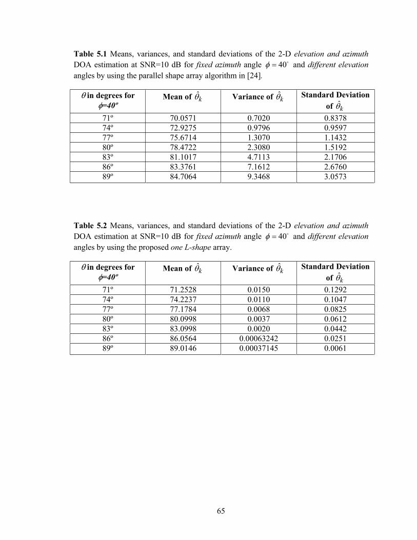
65
Table 5.1 Means, variances, and standard deviations of the 2-D elevation and azimuth
DOA estimation at SNR=10 dB for fixed azimuth angle 40 and different elevation
angles by using the parallel shape array algorithm in [24].
in degrees for
=40ºMean of k
ˆ Variance of kˆ Standard Deviation
of kˆ
71º 70.0571 0.7020 0.8378
74º 72.9275 0.9796 0.9597
77º 75.6714 1.3070 1.1432
80º 78.4722 2.3080 1.5192
83º 81.1017 4.7113 2.1706
86º 83.3761 7.1612 2.6760
89º 84.7064 9.3468 3.0573
Table 5.2 Means, variances, and standard deviations of the 2-D elevation and azimuth
DOA estimation at SNR=10 dB for fixed azimuth angle 40 and different elevation
angles by using the proposed one L-shape array.
in degrees for
=40ºMean of k
ˆ Variance of kˆ Standard Deviation
of kˆ
71º 71.2528 0.0150 0.1292
74º 74.2237 0.0110 0.1047
77º 77.1784 0.0068 0.0825
80º 80.0998 0.0037 0.0612
83º 83.0998 0.0020 0.0442
86º 86.0564 0.00063242 0.0251
89º 89.0146 0.00037145 0.0061

66
D. Simulation 4
From this simulation, Figures 5.6 and 5.7 show the standard deviation of the
azimuth and elevation angle estimation versus the SNR in dB for a single source of DOA
( 60,70 ), respectively. The total number of elements used is 15 for both methods. As
shown in Figure 5.6, the proposed one L-shape is slightly worse than the PM of the
parallel shape in [24] for the azimuth angle estimation. However, it can be seen from
Figure 5.7 that performance of the proposed one L-shape configuration gives much better
performance for elevation angle estimation, especially at a low SNR value, than the PM
[24] with the parallel shape.
Figure 5.6. Standard deviation of the azimuth angle estimation versus SNR for a single
source at (70º, 60º) by using both the parallel shape in [24] and the proposed one L-shape
array.

67
Figure 5.7. Standard deviation of the elevation angle estimation versus SNR for a single
source at (70º, 60º) by using both the parallel shape in [24] and the proposed one L-shape
array.
E. Simulation 5
From this simulation, Figure 5.8 shows the root mean square error (RMSE) versus
the SNR for the single source of DOA (68º, 60º). In [24], fifteen-elements were used for
the parallel-shape linear array. However, only ten elements were used for the proposed
one L-shape array. The RMSE for the joint DOA estimation is defined as
22 ˆˆERMSE . (5.40)
As observe, the proposed one L-shape algorithm, even with a smaller number of
antenna elements, can be 5 dB in SNR better than the parallel-shape in [24]. So, the
computational load and complexity can significantly be reduced by using a smaller
number of elements.

68
Figure 5.8. Root mean square error (RMSE) of joint elevation and azimuth angle
estimations versus SNR for a single source at (68º,60º) by using both the parallel shape
array with 15 elements and the proposed one L-shape array with 10 elements.
F. Simulation 6
From this simulation, Figures 5.9 and 5.10 show the RMSE in degrees for all
possible azimuth and elevation angle pairs , from 0º to 90º with 5º increments for
the proposed one L-shape and the parallel-shape algorithm in [24], respectively. It is
assumed that K=1 is the single-source signal and that the array structure contain a 15
elements. The 10 dB SNR and 500 trials were run, and 200 hundred snapshots per trial
were used. The maximum elevation angle was restricted to 90º for both algorithms, as
shown in Figures 5.9 and 5.10, because the maximum elevation angle in [24] was º,
whereas the maximum elevation angle in this algorithm is º.

69
Figure 5.9. Root mean square error (RMSE) of joint elevation and azimuth angle
estimations at SNR =10 dB for a single source at different (DOAs) by using proposed one
L-shape array with 15 elements in total.
Figure 5.10. Root mean square error (RMSE) of joint elevation and azimuth angle
estimations at SNR=10 dB for a single source at different (DOAs) using the parallel
shape with 15 elements
The principle reason why the proposed one L-shape method, as shown in Figure
5.9, showed no failure at elevation angles in the range of 90,70 , whereas the method

70
in [24] failed, is presented below. Also, the reason why the proposed one L-shape method
fails as both the azimuth and elevation angles approach 0º is given.
Equations (5.25) and (5.32) are for the elevation and azimuth angle estimations,
respectively, in the proposed one L-shape algorithm. Note that the estimation of the
elevation angle in equation (5.25) is obtained in the same way as ESPRIT [9], except for
the calculation of k,1ˆ which uses the PM method in the proposed method. Therefore, the
proposed one L-shape algorithm showed no failure for any SNR and any elevation angle,
as does ESPRIT. But the RMSE of estimation kˆ increases as the SNR decreases.
Substituting the estimation kˆ of elevation angle into equation (5.32) to estimate the
azimuth angle, the argument of the arc-cosine /)ˆsin2(
ˆarg ,2
k
kkx
d can be greater than unity
when both k and k are close to 0º, and estimation kkx,2
ˆ is imperfect due to the
noise. This is because kkx,2
ˆ is approximately equal to
kkkkd cossin2 , where k
and k
are estimation errors due to noise.
Hence, the arc-cosine argument /)ˆsin2(
ˆarg ,2
k
kkx
d can be written approximately as
k
kkkk
ˆsin
cossin whose absolute value can be greater than 1 with a nonzero
probability when the absolute value of kksin is larger than the absolute value of
kˆsin . This failure probability increases as k approaches 0º because
kkcos
approaches the maximum value. A similar reason justifies why the proposed one L-shape
using the y-axis can fail as k approaches 90º.

71
According to [26, Section III, Part C, (p. 2063) and Section IV, Part B, (p. 2064)]
the parallel shape algorithm fails when the elevation angle is between 70º and 90º. The
authors use the same DOA estimation equations as those used by [24] although they use a
different antenna array structure from that of the parallel-shape in [24].
Further analysis and more simulations found that the proposed one L-shape
algorithm is not superior to the parallel shape algorithm for all DOAs. The proposed one
L-shape algorithm can fail with 50 percent if both the azimuth and elevation angles
approach 0º. The failure rate decreases as the azimuth angle becomes larger than 0º.
Furthermore, the failure rate depends on the SNR. No failure was found when the
azimuth angle was larger than 5º for SNR=10 dB, regardless of the elevation angle. Note
that the failure rate of the parallel shape algorithm in [24] is also 50 percent when the
elevation angle is larger than 80º, regardless of the azimuth angle.
However, the proposed one L-shape algorithm has many advantages over the
parallel shape in [24]. First, the case of 0,0, occurs very rarely or not at all in a
cellular communications system because the practical elevation angles are close to 90º,
and also the 0º azimuth angle has a small antenna gain due to the side lobe effects of a
linear array. The practical range of the azimuth angle would be between 30º and 150º in a
three-sectored cellular communication system.
Second, the proposed one L-shape algorithm works well for these practical ranges
of angles. The ranges of the azimuth and elevation angles in the proposed one L-shape
algorithm are (0º, 360º) and (0º, 180º), respectively. However, the parallel-shape
algorithm in [24] fails, or does not work, in these practical cellular system environments
because the maximum range of the elevation angle in [24] is 90º.
72
Third, the average RMSE value of the proposed one L-shape algorithm is smaller
than that of the parallel shape algorithm in [24], as shown in Figures 9 and 10. The failure
events were not included in the RMSE calculation. For example, the average RMSE
values of the proposed one L-shape and the parallel-shape algorithm in [24] are 0.8021
and 0.9335 degrees, respectively, under the simulation environments shown in Figures 9
and 10.
Fourth, the proposed one L-shape algorithm has another practical advantage over
the existing parallel shape in [24]. For example, the proposed one L-shape algorithm does
not require any pair matching between the azimuth and elevation angle estimations. The
pair matching requirement in [24] causes a high complexity and exhaustive search when
the number of sources is large.
G. Simulation 7
From this simulation, Figures 5.11 shows the corresponding RMSE in degrees for
all possible azimuth and elevation angle pairs , from 0º to 90º with 5º increments for
the proposed two L-shape algorithm in Section 5.3 with the same parameters used for the
results in Figures 5.9 and 5.10. Figure 5.11 shows that the RMSE in degrees of the
proposed two L-shape algorithms is only .4707 degrees, which is smaller than those of
the proposed one L-shape and the parallel shape in [24]. Furthermore, no failure occurs
for all pair angles with the proposed two L-shape algorithm, whereas a 50 percent failure
occurs for some pair angles with the proposed one L-shape and the parallel one in [24].
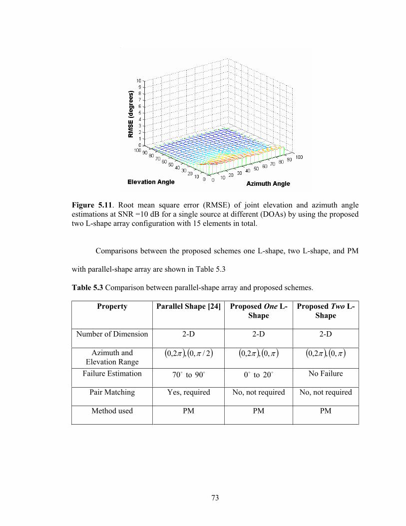
73
Figure 5.11. Root mean square error (RMSE) of joint elevation and azimuth angle
estimations at SNR =10 dB for a single source at different (DOAs) by using the proposed
two L-shape array configuration with 15 elements in total.
Comparisons between the proposed schemes one L-shape, two L-shape, and PM
with parallel-shape array are shown in Table 5.3
Table 5.3 Comparison between parallel-shape array and proposed schemes.
Property Parallel Shape [24] Proposed One L-
Shape
Proposed Two L-
Shape
Number of Dimension 2-D 2-D 2-D
Azimuth and
Elevation Range 2/,0,2,0 ,0,2,0 ,0,2,0
Failure Estimation 70 to 90 0 to 20 No Failure
Pair Matching Yes, required No, not required No, not required
Method used PM PM PM

74
5.5 Summary
In this chapter, two 2-D azimuth and elevation angle estimation algorithms, called
one L-shape and two L-shape algorithms, were proposed using the PM. These methods,
even with fewer numbers of elements, can estimate much better than the PM of the
parallel shape array in [24]. In addition, both the proposed one and two L-shape
algorithms do not require any pair matching for 2-D DOA estimation problems, whereas
the parallel shape PM in [24] does require pair matching. Furthermore, the proposed two
L-shape algorithm shows no failure for all pair angles, whereas the proposed one L-shape
and the parallel one in [24] have a 50 percent failure for some pair angles.

75
CHAPTER 6
2-D DOA ESTIMATION WITH NO FAILURE AND NO EIGEN
DECOMPOSITION
The previous chapter introduced the 2-D DOA estimation by using the one or two
L-shape array configuration. This chapter proposes an antenna array configuration for 2-
D DOA estimation and proves its performance. The objective of the proposed method in
this chapter is to overcome the failure of DOA estimation and improve the performance
compared to PM [24]. In addition, the proposed method has less computational load
compared to PM [24].
6.1 Introduction
Many efforts have been made to reduce the computational complexity of the EVD
[71-74]. However, these techniques still require high computational complexity. Marcos
proposed another DOA estimation scheme, called a propagator method (PM), without
using any EVD or SVD [31-34] for one-dimensional DOA estimation. The PM method
can reduce the computational complexity to order O(2NLK) with insignificant signal-to-
noise ratio (SNR) degradation [31-34, 75], where K is the number of sources and N is the
number of antenna elements in a subarray. Li et al. extended the PM in [31] to a 2-D
DOA estimation problem [76]. But the drawback of Li’s method is that it requires an
exhaustive 2-D peak search through all possible steering vectors.
Recently, Wu et al. proposed a 2-D DOA estimation method using two parallel
uniform linear arrays (ULAs), which were divided into three subarrays, X, Y, and Z, as
shown in Figure 6.1 [24]. The Wu method does not require the 2-D peak search;
therefore, it has a significantly lower computational complexity than the one used by Li

76
et al. [18]. But the Wu method [24] has several drawbacks: (1) it requires a pair matching
between the 2-D azimuth and elevation angle estimations; (2) it has an estimation failure
problem when the elevation angles are between 70 and 90 ; and (3) it has performance
degradation at low SNRs, especially when the elevation angles are between 0 and 20
and the azimuth angles are close to 0 .
.
x
y
Z
elementreferenece )0,0( ),0( d
)0,(Nd
)0,)1(( dN
),)1(( ddN
Zsubarray
Ysubarray
Xsubarray
),( dd
)0,(d
Figure 6.1. Array configuration used for the joint elevation and azimuth , DOA
estimation by the method in [24].

77
6.2 Proposed Antenna Array Configuration for 2-D DOA Estimation
A. System Model and Analysis
Figure 6.2 shows the proposed array configuration, which consists of three
uniform linear arrays with interspacing d equal to a half wavelength of incident signals
where all sources use the same carrier frequency. The three uniform linear arrays shown
in Figure 6.2 consist of N, N+1, and N elements. One array is placed in the x-y plane,
another on the y-axis, and the last one in the y-z plane. Let X, Y, Z, and W denote the 1st,
2nd
, 3rd
, and 4th
subarrays respectively of the proposed array configuration shown in
Figure 6.2. Each subarray consists of N elements. Suppose that there are K narrowband
sources where the k-th source has an elevation angle k and an azimuth angle k , k=1,…,
K.

78
x
y
Z
elementreferenece
),0,0( d
),,0( dd ),)1(,0( ddN
)0,0,0( )0,,0( d )0,,0( Nd
)0,0,(d
)0,,( dd
)0,)1(,( dNd
Zsubarray
Ysubarray
Xsubarray
Wsubarray
Figure 6.2. Proposed array configuration used for the joint elevation and azimuth ,
DOA estimation.
The N×1 signal vectors received at the X, Y, Z, and W subarrays at snapshot t are
denoted, respectively, as
T
N txtxtxtX ...21 , (6.1)
T
N tytytytY 132 ... , (6.2)

79
T
N tztztztZ ...21 , (6.3)
T
N twtwtwtW ...21 , (6.4)
t=1,2…,L where superscript T represents the transpose, t the snapshot index, and L the
number of snapshots. These N×1 received vectors at snapshot t can be written as
tntSAtX x, (6.5)
tntSAtY y,, 1 (6.6)
tntSAtZ z2, (6.7)
tntSAtW w,, 3 (6.8)
where
KKaaaA ,...,,, 2211 (6.9)
TN
kkkk uua 1...1, , k=1,…, K (6.10)
kkk
dju
sinsin2exp (6.11)
T
K tstststS ...21 (6.12)
whereT
K,,1 ,T
K,,1 , S(t) is a signal vector at snapshot t for the K
sources, and nx, ny, nz, and nw are the N×1 additive white Gaussian noise vectors whose
elements have a zero mean and a variance of 2 .

80
The matrices ),(1 in equation (6.6), )(2 in equation (6.7), and ,3
in equation (6.8) are KK diagonal matrices containing information about the elevation
angle k and the azimuth angle k , which can be written as
kqqqdiag ...),( 211 (6.13)
kkk
djq
sinsin2exp (6.14)
krrrdiag ...)( 212 (6.15)
kk
djr
cos2exp (6.16)
kvvvdiag ..., 213 (6.17)
kkk
djv
cossin2exp (6.18)
respectively, where diag means the diagonal elements of the matrix.
The matrices ),(1 , )(2 , and ,3 can be found by employing the PM
[31, 24], whose computational complexity is smaller than that of the subspace eigenvalue
analysis such as MUSIC and ESPRIT algorithms. The PM in [18] makes a partition of the
array response vector A as
TTT AAA 21 (6.19)
where 1A and 2A are submatrices of dimension KK and KKN , respectively.
The K×(4N-K) propagator matrix P can be applied to the observation output vectors X, Y,
Z, and W in equations (6.5), (6.6), (6.7), and (6.8), respectively. D can be denoted
TTTTT AAAAD 321 . (6.20)
After partitioning D in a similar way, the equation can be written as
81
TTT DAD 11 (6.21)
where
TTTTTTTT AAAAAAAD 32312221121121 . (6.22)
Under the hypothesis that 1A is a K×K non-singular matrix, which most subspace based
methods assume when N 2K, the K×(4N-K) propagator matrix P is a unique linear
operator which can be written as
11 DAPH (6.23)
where the superscript H is the Hermitian operator, i.e., the conjugate and transpose.
The r(t) can denote a 4N×1 snapshot data vector written as
TTTTT tWtZtYtXtr , t=1,…, L. (6.24)
F can denote the 4N×L data matrix consisting of L snapshots as
.)(...),2(),1( LrrrF (6.25)
Then, the 4N×4N cross spectral matrix can be written as
HFFL
R1ˆ . (6.26)
The partitions of the data matrix F and cross-spectral matrix R̂ can be written,
respectively, as
2
1
F
FF (6.27)
and
JER̂ (6.28)
82
where 1F and 2F are sub-matrices with dimension LK and LKN )4( ,
respectively, and E and J are sub-matrices with dimension KN4 and KNN 44 ,
respectively.
Let dataP̂ and csmP̂ denote the K×(4N-K) and K×(4N-K) propagator-estimate
matrix based on the data matrix F and cross-spectral matrix R̂ , respectively. The
propagator-estimate matrix can be obtained by minimizing the following cost functions to
2
12ˆˆ
F
H
datadatadata FPFP (6.29)
2ˆˆ
Fcsmcsmcsm PEJP (6.30)
whereF
denotes the Frobenius norm. The optimum propagator-estimate matrix can be
found by applying the least square method on equations (6.29) and (6.30) as
HH
data FFFFP 21
1
11ˆ (6.31)
JEEEP HH
csm
1ˆ . (6.32)
Either dataP̂ or csmP̂ can be partitioned as
TTTTTTTTH PPPPPPPP 7654321ˆˆˆˆˆˆˆˆ (6.33)
where the dimension of 1P̂ , 2P̂ , 3P̂ , 4P̂ , 5P̂ , 6P̂ , and 7P̂ are identical with the dimension
of 2A , 11A , 12A , 21A , 22A , 31A and 32A ,respectively.
According to equation (6.23), and using equations (6.22) and (6.33), the following
equations can be written as

83
211ˆ AAP (6.34)
1112ˆ AAP (6.35)
1213ˆ AAP (6.36)
2114ˆ AAP (6.37)
2215ˆ AAP (6.38)
3116ˆ AAP (6.39)
3217ˆ AAP (6.40)
Using pair equations (6.34), (6.36); (6.34), (6.38); and (6.34), (6.40), 1 , 2 , and
3 can be found by solving the following formulas, respectively:
122
#
13ˆˆ AAPP (6.41)
222
#
15ˆˆ AAPP (6.42)
322
#
17ˆˆ AAPP (6.43)
where # denotes the pseudoinverse.
This implies that the diagonal elements in the diagonal matrices 1 , 2 , and 3 ,
respectively, can be estimated, i.e., by finding the K eigenvalues of each matrix #
13ˆˆ PP ,
#
15ˆˆ PP , and #
17ˆˆ PP in equations (6.41) to ( 6.43). Also, 1 , 2 , and 3 can be found
another way, i.e., by finding the eigenvalues of 2P̂ , 4P̂ , and 6P̂ in equations (6.35),
(6.37), and (6.39), respectively. Using #
13ˆˆ PP , #
15ˆˆ PP , and #
17ˆˆ PP yields more accurate results
than using 2P̂ , 4P̂ , and 6P̂ , but the former requires computation loads larger than the

84
later. Then, the azimuth and elevation angle estimates for each source can be easily found
as
kk
kkk
3
11
arg
argtanˆ (6.44)
kkk
kkk ˆcosarg
argtanˆ
2
31 (6.45)
using 1 , 2 , and 3 in (6.13), (6.15), and (6.17).
B. Discussion
Note that the elevation angle estimate kˆ can be found from equation (6.45) using
the azimuth angle estimate kˆ in equation (6.44). Both of these equations use the arc-
tangent operator, which allows the value of its argument to be larger than the unity. One
of the main advantages of the proposed method over the method in [24] is that form uses
the arc-tangent operator for estimation of kˆ and k
ˆ from different sources. These arc-
tangent operations allow no estimation failure. In other words, the arc-tangent
operation, )(tan 1 xy , is a one-to-one function for the range of 2
,2
y and all
x , where denotes the real field domain. This implies that the arc-tangent values
always exist for any x , and the proposed method never fails.
However, the method in [24, equation (22.14)] estimates the azimuth and
elevation angles as

85
k
k
k
,3
,11
arg
argtanˆ (6.46)
2
,3
2
,1
1 argarg2
sinˆkkk
d (6.47)
where, for convenience, the notations in [22, eq. (22.14)] were changed to match the
proposed notations. Note that equation (6.47) of the method in [24] uses arc-sine to
estimate the elevation angle. This arc-sine function, )(sin 1 xy , is a one-to-one function
only for 1,1x and2
,2
y . In practice, the absolute value x can be larger
than one, even if the SNR is high, such as 10 dB. This situation most likely occurs when
the elevation angles are between 70 and 90 , which is a practical range in a mobile
environment. Moreover, the failure rate increases to 50 percent when the elevation angle
in [24] approaches 90 . The explanations are explained in [24, 25].
The computational loads of the proposed method are then compared to those of
the method in [24] using the same number of array elements in total, Mtotal. The number
of multiplications in [24] is in the order of LKNO 3 to compute the propagator per trial,
where N is the number of elements in each subarray as shown in Figure 6.1,
1'2NM total , L is the number of snapshots per trial, and K is the number of sources.
The proposed method uses an order of NLKO 4 multiplications to compute the
propagators in equation (6.31) or (6.32) per trial, where N is the number of elements in
each subarray of the proposed array configuration shown in Figure 6.2, where NN
and 13NM total . For example, if the total number of elements is 31totalM , then N
will be 15 and the computational load for the method in [24] will be on order of
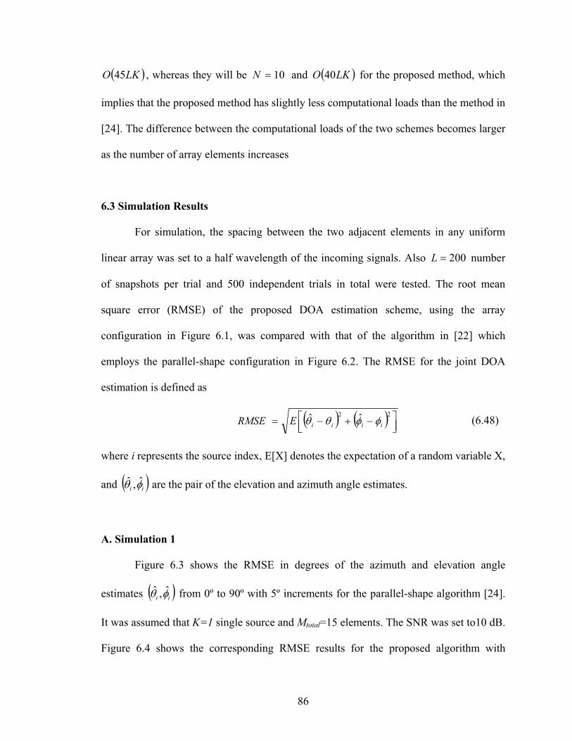
86
LKO 45 , whereas they will be 10N and LKO 40 for the proposed method, which
implies that the proposed method has slightly less computational loads than the method in
[24]. The difference between the computational loads of the two schemes becomes larger
as the number of array elements increases
6.3 Simulation Results
For simulation, the spacing between the two adjacent elements in any uniform
linear array was set to a half wavelength of the incoming signals. Also 200L number
of snapshots per trial and 500 independent trials in total were tested. The root mean
square error (RMSE) of the proposed DOA estimation scheme, using the array
configuration in Figure 6.1, was compared with that of the algorithm in [22] which
employs the parallel-shape configuration in Figure 6.2. The RMSE for the joint DOA
estimation is defined as
22 ˆˆiiiiERMSE (6.48)
where i represents the source index, E[X] denotes the expectation of a random variable X,
and iiˆ,ˆ are the pair of the elevation and azimuth angle estimates.
A. Simulation 1
Figure 6.3 shows the RMSE in degrees of the azimuth and elevation angle
estimates iiˆ,ˆ from 0º to 90º with 5º increments for the parallel-shape algorithm [24].
It was assumed that K=1 single source and Mtotal=15 elements. The SNR was set to10 dB.
Figure 6.4 shows the corresponding RMSE results for the proposed algorithm with

87
Mtotal=13 elements. Figures 6.3 and 6.4 show that the proposed algorithm improves the
performance significantly compared to the parallel-shape array in [24]. The average of
the RMSE value over all possible pairs iiˆ,ˆ for the proposed algorithm was .3923 in
degrees whereas that for the parallel-shape algorithm in [24] was 0.9335 in degrees. In
Figures 6.3 and 6.4 only the successful trial cases were counted for the RMSE
calculation. It was observed that the parallel-shape array in [24] shows many estimation
failures when the elevation angles were between 70 and 90 . As the elevation angle
approaches 90 , the estimation failure rate of the parallel-shape array becomes 50
percent.
Figure 6.3. RMSE of joint elevation and azimuth angle estimations at SNR=10 dB for a
single source, using the parallel shape [24] with Mtotal=15 elements.

88
Figure 6.4. RMSE of joint elevation and azimuth angle estimations at SNR=10 dB for a
single source, using the proposed configuration with Mtotal=13 elements.
However, the proposed algorithm shows zero number of estimation failures for
any pair of incident DOAs ii , and all trials. Refer to equations (6.44) and (6.45) to
see the reasons why the PM algorithm with the proposed antenna array configuration in
Figure 6.2 shows no failures. Therefore, the PM method with the proposed antenna array
configuration in Figure 6.2 is more practical than the PM of the parallel-shape in [24],
because typical elevation angles are between 70 and 90 in a mobile communications
environment [77, p.19].
B. Simulation 2
From this simulation, Tables 6.1 and 6.2 list the RMSE values and the number of
estimation failures for both PMs with the parallel-shape in Figure 6.1 [24] and the
proposed shape in Figure 6.2, respectively, with an elevation angle as a parameter from
72º to 90º, with a 3º increment for a given azimuth angle of 60º. A single source and three

89
different SNR values (-5, 0, and 5 dB) were considered. The proposed configuration
gives a better estimation than the parallel-shape array [24] because the RMSE of the
proposed method was approximately 2º smaller than that of the parallel-shape array. In
addition, Table 6.2 confirms that the proposed antenna array configuration showed no
estimation failure regardless of SNR values, but the RMSE increases as SNR decreased.
Table 6.1 indicates that the parallel shape array shows an unacceptable estimated failure
rate, as the SNR value becomes low or the elevation angle approaches 90º. Moreover, the
estimation failure rate of the parallel-shape array was almost 50 percent when the
elevation angle approached 90º.
Table 6.1 RMSE and the number of the failures for the 2-D elevation and azimuth DOA
estimation using the parallel shape configuration when azimuth angle 60 and
elevation angle varies from 72 to 90 . Five hundred independent trials have been
tested.
, RMSE
SNR= -
5dB
RMSE
SNR= 0
dB
RMSE
SNR= 5
dB
# Failures
SNR= -
5dB
# Failures
SNR= 0
dB
# Failures
SNR= 5
dB
72,60 4.5025 2.5052 1.6152 10 0 0
75,60 4.5687 2.7188 1.7552 40 0 0
78,60 4.5866 3.1364 1.8896 110 20 3
81,60 4.4885 3.2186 2.3984 154 147 25
84,60 4.5381 3.1971 2.5603 190 178 100
87,60 4.4828 3.2561 2.5687 246 260 110
90,60 4.5213 3.2312 2.6372 270 271 237

90
Table 6.2 RMSE and the number of the failures for the 2-D elevation and azimuth DOA
estimation using the proposed shape configuration when azimuth angle 60 and
elevation angle varies from 72 to 90 . Five hundred independent trials have been
tested.
, RMSE
SNR= -
5dB
RMSE
SNR= 0
dB
RMSE
SNR= 5
dB
# Failures
SNR= -
5dB
# Failures
SNR= 0
dB
# Failures
SNR= 5
dB
72,60 2.5704 1.1601 .6504 0 0 0
75,60 2.5946 1.1291 .5894 0 0 0
78,60 2.4496 1.0891 .5823 0 0 0
81,60 2.2648 1.0641 .5061 0 0 0
84,60 2.2486 .9401 .4915 0 0 0
87,60 2.1871 .9532 .4723 0 0 0
90,60 2.1928 .9321 .4643 0 0 0
C. Simulation 3
Figures 6.4 and 6.5 show the RMSE values of the joint elevation and azimuth
DOA estimation versus the SNR in dB for source 1 and 2, respectively, when K=2 source
signals arrive with DOAs of ( , )=(15 , 6 ) and (30 , 50 ). The total number of elements
was Ntotal=13 for both the proposed and parallel shape configurations. It was observed
that the proposed configuration is 5.4 dB and 2.5~3.3 dB better in SNR than the parallel
shape in [24] for Source 1 and Source 2, respectively, at a given RMSE value, e.g., 0.5
or 1 .
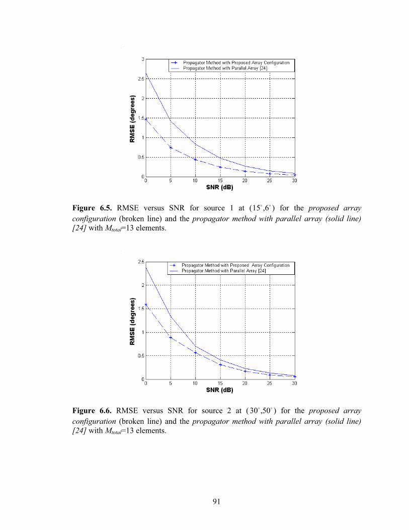
91
Figure 6.5. RMSE versus SNR for source 1 at ( 6,15 ) for the proposed array
configuration (broken line) and the propagator method with parallel array (solid line)
[24] with Mtotal=13 elements.
Figure 6.6. RMSE versus SNR for source 2 at ( 50,30 ) for the proposed array
configuration (broken line) and the propagator method with parallel array (solid line)
[24] with Mtotal=13 elements.

92
6.4 Summary
In this chapter, an antenna array configuration was proposed for the 2-D azimuth
and elevation angle estimation problem and compared with the parallel-shape
configuration. The proposed method employed a PM, which does not require any EVD or
SVD but only a linear operation. The proposed 2-D DOA estimation scheme shows a
significant improvement over the existing parallel shape scheme in [24]. In other words:
(1) the proposed scheme did not require any pair matching for the 2-D DOA estimation
problems whereas the parallel shape PM scheme in [24] did; and (2) the proposed
algorithm showed no estimation failure whereas the parallel-shape method in [24] could
have a 50 percent failure.

93
CHAPTER 7
1-D DOA ESTIMATION OF CORRELATED SOURCES WITH UNKNOWN,
SPATIALLY UNCORRELATED AND NONSTATIONARY NOISE
In the previous chapters, the proposed methods for 1-D and 2-D DOA estimation
assume that the noise is spatially white Gaussian noise of a known covariance matrix. In
some situations, the additive sensor noise may not be known. This chapter proposes a
method of DOA estimation for correlated sources for this kind of situation. For example,
the unknown noise environment is spatially uncorrelated and nonstationary from one
antenna element to another, which means that the additive white noise has different
power at each antenna element and is uncorrelated. The performance of the proposed
method is compared to that in [37], where the same noise environment was assumed but
only uncorrelated sources were considered. The proposed method employs the difference
matrix between the forward-backward averaging covariance matrix of the received data
and its transformation. This difference matrix was used to eliminate the effects of the
noise components on the array structure. The proposed algorithm showed better
performance when the sources were correlated [37].
7.1 Introduction
Most of the methods for direction of arrival angle (DOA) estimation with array
processing assume spatially white Gaussian noise of a known covariance matrix [9, 14].
However, the additive sensor noise in some situations may not be known. To estimate the
DOAs of the signals with an unknown covariance matrix, several algorithms have been
proposed. For example, Paulraj and Kailath assumed that the unknown noise covariance

94
matrix is invariant across the two measurements under any array rotation [36]. Prasad and
Chandra introduced a difference covariance matrix between the original covariance
matrix of the received signals at the array and its transformation, by assuming that the
covariance matrix is a symmetric Toeplitz. This implies that the noise is spatially
correlated among sensors but still unknown [35]. Moghaddaamjoo assumed that the white
noises at the array elements are not spatially stationary but uncorrelated, which implies
that the covariance matrix is a diagonal matrix of unknown and unequal noise power
[37]. These algorithms [35-37] assumed uncorrelated incident sources. Therefore, they
likely fail in the scenarios when the multiple incident sources of different (DOAs) are
partially or fully correlated, e.g., coherent.
The proposed method is to present a DOA estimation scheme for correlated
sources including uncorrelated ones under an unknown, spatially uncorrelated and
spatially nonstationary noise environment. It is assumed that the unknown covariance
noise matrix is diagonal with unequal noise power on the diagonal as the one in [37].
The proposed method uses a forward-backward (FB) averaging covariance
matrix, which has the effect of doubling the number of snapshots of the information data,
and able to decorrelate the correlated sources [78-84, 68]. The proposed algorithm takes
the difference between the FB covariance matrix and its transform instead of the FB
alone. In this way, the effects of the unknown noise on the array structure can be
eliminated without having any degradation on the signal components and can improve the
performance of the DOA estimation.

95
7.2 System Model
A uniform linear array (ULA) composed of M sensors and K narrowband signals
of the different DOAs K,...,1 was considered. Then, an observed snapshot from the M
array elements was modeled as
)(n)(s)(X ttAt (7.1)
where KA a,...,a 1 is an KM matrix of array response vectors )(s t is an 1K
signal vector, tn is an 1M noise vector, is the wavelength of the signal, and d is
the interspacing distance between the elements.
The array covariance matrix R of the received signal vector in the forward
direction can be written as
QAARtXtXER H
SH (7.2)
where Q is an MM noise covariance matrix, )()( tstsER HS is the KK source
covariance matrix, and the superscript H represents the Hermitian operation. An
estimate R̂ of the covariance matrix is given as
HL
k
kkL
R XX1ˆ
1
. (7.3)
The matrix R is called centrohermitian if the following condition is satisfied [85]
as
JJRR (7.4)
where J represents the exchange matrix, i.e., 1’s on the antidiagonal and 0’s elsewhere
as

96
01
.
.
10
J (7.5)
and the superscript * stands for the complex conjugate.
The proposed method employs the FB averaging for the covariance matrix of the
observation data. Here, the forward covariance matrix is obtained from equation (7.3) and
the backward covariance matrix is JJR . This FB averaging has two advantages: (1) it is
equivalent to doubling the number of snapshots of the data, and (2) correlated sources can
be decorrelated. The FB averaging can be written as [68], 79]
JRJRRFBˆˆ
2
1. (7.6)
Assuming that the unknown covariance noise matrix is diagonal with equal or
unequal noise power on the diagonal as explained in [37], the proposed scheme can
eliminate the noise effects on the array structure and can give better performance,
compared with the one in [37], by taking the difference R between the transformation of
FBR and the original FBR . The transformation of the FB can be done without having any
effects on the signal components as follows.
Let B be any real diagonal matrix whose diagonal elements are different from
each other, i.e., ),(),( jjBiiB for all ji . For example, the matrix B for numerical
analysis can be chosen as follows:
)1(0000
0.000
00.00
0000
00001
M
B (7.7)

97
where is any real number between 1 and -1. Then, Q can be pre-multiplied with 1B
and post-multiplied with B , which will not make any changes in the value of Q ,
assuming that Q is another any diagonal matrix. In other words, we can write
QBQBQBB 11 . (7.8)
The proposed algorithm takes equation (7.6) and another property, QJQJ or
QQJJQ ** , and obtains a new transform of the FB array covariance matrix. By
pre- and post-multiplying FBR with 1B and B , and by subtracting the original FBR from
it, R can be obtained as
JJRRBJJRRBR2
1
2
11 . (7.9)
Note that the method in [37] employs )( 11 RBBBRBjR , where 1j . This
method will fail when the sources are correlated because R does not have a full rank
whereas the R in equation (7.9) can be chosen to have a full rank. The conditions for R
to have a full rank are summarized as follows:
Theorem: If RFB in equations (7.6) has a full rank and the diagonal elements of B are
different from each other, i.e., )j,j(B)i,i(B for all ji and KM 2 , then R in
equation (7.9) has a full rank.
Proof: This theorem can be proved by using equation (7.15).
Note that the condition for RFB to have a full rank can be achieved by the forward
and backward averaging process even when R does not have a full rank due to the
correlated sources. In addition, note that the diagonal elements of R are all zero. This

98
implies that the effects of any spatially nonstationary, white, and unknown noise will be
removed.
Substituting in equation (7.2) into equation (7.9) to derive equation (7.15) as
JJQARJAQAARBJJQJARJAQAARBR H
S
H
S
H
S
H
S2
1
2
11
(7.10)
Using the properties of QJJQ for any diagonal covariance matrix Q with unequal or
equal noise power and QQBB 1 , equation (7.10) can be written as
JJQASJRQAARBQJARJAAARBR H
S
H
S
H
S
H
S2
12
2
11
JARJAAARBJARJAAARB H
S
H
S
H
S
H
S2
1
2
1 1. (7.11)
By substituting
aa cos)1()/2( MdjeJ (7.12)
into equation (7.11), equation (7.12) can be written as
HH
SS
HH
SS ADDRRABADDRRABR2
1
2
1 1 (7.13)
where
eediagD KMjMj cos1/21cos1/2 . (7.14)
Note that the covariance matrix Q of the unknown noise is completely removed in
equation (7.14).
Equation (7.14) and some algebraic manipulation can be used to obtain

99
H
H
SS
H
SS
BAA
DDRR
DDRRABAR
02
12
10
*
1 (7.15)
Based on the assumption that KM 2 and A has a full rank of K, then
][ 1ABA also has a full column rank of 2K. The eigenvalue decomposition (EVD) for
R in equation (7.15) can be used to find the DOAs. The EVD will yield K2 nonzero
eigenvalues and KM 2 zero eigenvalues. The eigenvectors ei corresponding to the
KM 2 eigenvalues will span the null subspace, these eigen vectors are orthogonal to
the space of ][ 1ABA . Hence, from the null subspace eigenvectors of R with the
MUSIC algorithm [14], the DOAs can be estimated by using the a power spectrum
M
Ki
H
ii
HH
ii
H BBKM
P
12
1 )aeeaaeea(2
1
1 (7.16)
where the peaks of P indicate the DOAs for the incident sources. Here
MKE e,...,e 12 denotes the null subspace eigenvectors of R .
7.3 Numerical Results
Performance of the proposed algorithm is compared to that of the method in [37]
through the numerical analysis of three cases: Case (1) uncorrelated sources, Case (2)
correlated sources, and Case (3) mixed sources of correlated and uncorrelated sources
under an unknown noise environment with an unequal diagonal covariance matrix. For
the noise covariance matrix Q, it is assumed that the second and eighth diagonal elements
are 2 and 4, respectively, and the others are 1. In addition, two and three number of
sources of different DOAs are considered, in addition to a ULA consisting of eight

100
sensors 8M with spacing equal to a half wavelength, and in (8) for B matrix is set
to 9. . Two cases of source power equal to -5 dB and -7 dB are assumed.
A. Simulation 1
For the set of results shown in Figures 7.1 and 7.2, two uncorrelated signals were
received with azimuth DOAs at 120,110, 21 and a -5 dB source power for all
sources. Figures 7.1 and 7.2 show the power spectrum versus the azimuth DOA angle for
the two uncorrelated sources that are 10 degrees apart. It becomes clear in these Figures
that both the proposed algorithm and the one in [37] give accurate DOA estimations for
all sources, i.e., two peaks are observed accurately at the true DOAs of 110º, 120º when
the sources are uncorrelated.
Figure 7.1. Power spectrum of DOA estimations for two noncoherent sources at [110º,
120º] with source power = [-5 -5] dB, respectively, and 8M elements, by using the
proposed method.

101
Figure 7.2. Power spectrum of DOA estimations for two noncoherent sources at [110º,
120º] with source power = [-5 -5] dB, respectively, and 8M elements, by using the
method in [37].
B. Simulation 2
The set of results shown in Figures 7.3 and 7.4 assume a different source power
equal to -7 dB and azimuth DOAs at 80,70 . These Figures show the power spectrum
versus the azimuth angle for two fully correlated (coherent) sources. Figure 7.3 shows
that the proposed algorithm gives accurate DOAs estimations at 80,70 , whereas in
Figure 7.4, the method in [37] completely fails to detect any of the two sources. In
addition, many false peaks occurred at incorrect angles, none of which gave correct DOA
estimations.

102
Figure 7.3. Power spectrum of DOA estimations for two coherent sources at [70º, 80º]
with source power = [-7 -7] dB, respectively, and 8M elements, by using the
proposed method.
Figure 7.4. Power spectrum of DOA estimations for two coherent sources at [70º, 80º]
with source power = [-7 -7] dB, respectively, and 8M elements, by using the method
in [37].
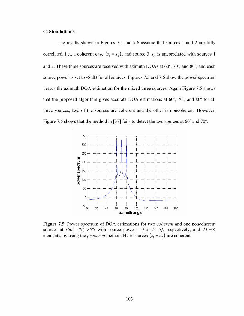
103
C. Simulation 3
The results shown in Figures 7.5 and 7.6 assume that sources 1 and 2 are fully
correlated, i.e., a coherent case 21 ss , and source 3 3s is uncorrelated with sources 1
and 2. These three sources are received with azimuth DOAs at 60º, 70º, and 80º, and each
source power is set to -5 dB for all sources. Figures 7.5 and 7.6 show the power spectrum
versus the azimuth DOA estimation for the mixed three sources. Again Figure 7.5 shows
that the proposed algorithm gives accurate DOA estimations at 60º, 70º, and 80º for all
three sources; two of the sources are coherent and the other is noncoherent. However,
Figure 7.6 shows that the method in [37] fails to detect the two sources at 60º and 70º.
Figure 7.5. Power spectrum of DOA estimations for two coherent and one noncoherent
sources at [60º, 70º, 80º] with source power = [-5 -5 -5], respectively, and 8M
elements, by using the proposed method. Here sources 21 ss are coherent.
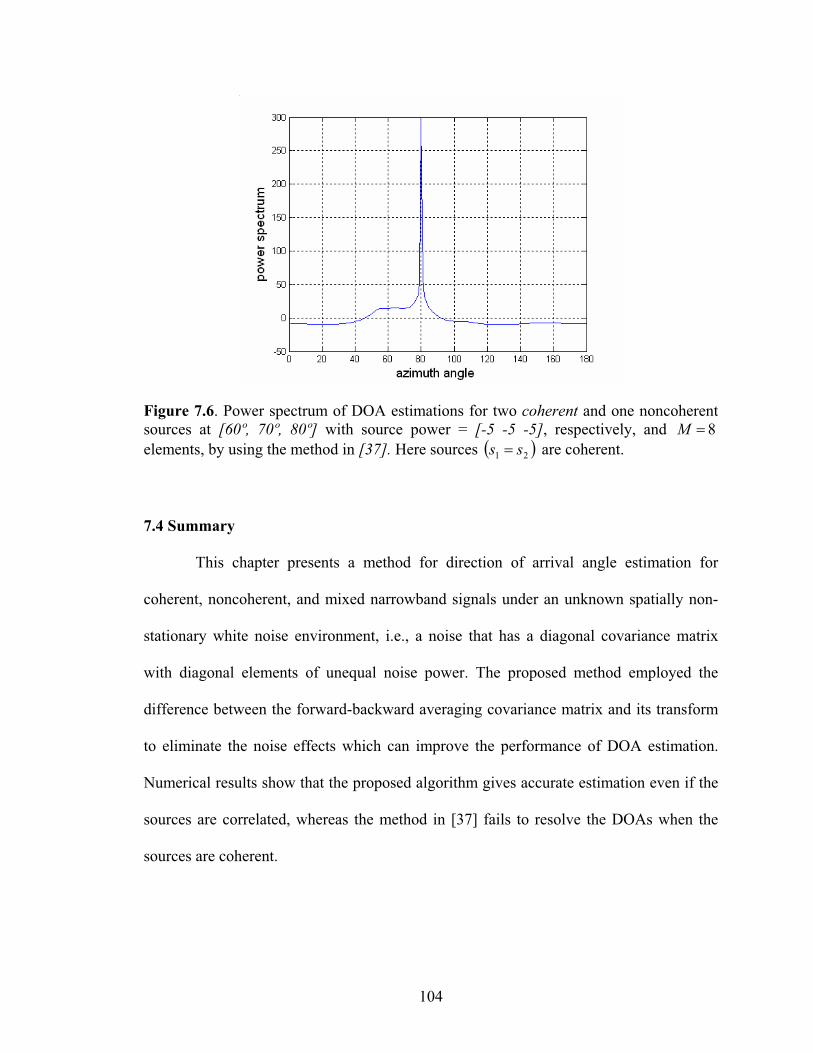
104
Figure 7.6. Power spectrum of DOA estimations for two coherent and one noncoherent
sources at [60º, 70º, 80º] with source power = [-5 -5 -5], respectively, and 8M
elements, by using the method in [37]. Here sources 21 ss are coherent.
7.4 Summary
This chapter presents a method for direction of arrival angle estimation for
coherent, noncoherent, and mixed narrowband signals under an unknown spatially non-
stationary white noise environment, i.e., a noise that has a diagonal covariance matrix
with diagonal elements of unequal noise power. The proposed method employed the
difference between the forward-backward averaging covariance matrix and its transform
to eliminate the noise effects which can improve the performance of DOA estimation.
Numerical results show that the proposed algorithm gives accurate estimation even if the
sources are correlated, whereas the method in [37] fails to resolve the DOAs when the
sources are coherent.

105
CHAPTER 8
1-D AND 2-D DOA ESTIMATION WITH PROPAGATOR METHOD FOR
CORRELATED SOURCES UNDER UNKNOWN SYMMETRIC TOEPLITZ
NOISE
8.1 1-D DOA Estimation with Forward-Backward Averaging
In the previous chapter a method was proposed for DOA estimation for
correlated sources under a spatially uncorrelated and nonstationary noise environment,
which means that the additive white noise had different power at each antenna element
and was uncorrelated. In some situations, the noise field consists of a set of point sources
distributed symmetrically broadside about the array. This situation is valid when the
noise field is cylindrically or spherically isotropic. Then, the unknown noise covariance
matrix will be a symmetric Toeplitz matrix, which was studied in [35].
This chapter shows use of the propagator method to find the direction of arrival
angles from the incident sources without any eigenvalue decomposition. This can reduce
the complexity when compared to the eigenvalue subspace method such as a MUSIC
algorithm with persymmetrization which requires the eigenvalue decomposition or
singularvalue decomposition. Also, the proposed algorithm is applied to a situation when
the incident sources are uncorrelated or coherent in pairs.
The unknown covariance noise matrix is assumed to be in a symmetric Toeplitz
form, similar to the Prasad’s noise model [35]. But when compared with the Prasad’s
method, the proposed method has two main advantages: (1) it does not require any
eigenvalue decomposition to find the DOAs, as does Prasad’s, and (2) the proposed
algorithm requires the number of sensors M to be larger than the number of sources K ,
i.e., KM , whereas the method in [35, 37] requires KM 2 . Therefore, the proposed

106
method can take a general situation of KM , where the Prasad’s method fails for
KMK 2 case. The proposed method is based on a covariance matrix difference
between the average of the forward-backward covariance matrices of the received data
and the Hermition of the backward. This difference is introduced to eliminate the noise
components from the array structure. It will be verified that that the proposed method
gives better performance and less computation than a MUSIC algorithm with
persymmetrization and the conventional MUSIC.
8.1.1 Introduction
Prony and Matrix Pencil algorithms were applied directly to the data to find the
DOA estimation for incident sources [86]. These algorithms are inferior to the proposed
method because the observations are corrupted by noise vectors that are not eliminated
and can degrade the performance. This chapter proposes a new covariance matrix
difference method based on the cross-correlation matrix of the received data. The
proposed algorithm considers a special unknown noise environment whose covariance
matrix is in a Toeplitz form [35]. In this situation, the proposed method is not influenced
by noise. In other words, its noise covariance matrix can completely be eliminated, thus
improving definitely and making the proposed method work well even at very low SNR
values, such as -5 dB. The Prony and Matrix Pencil algorithms cannot cancel the noise
effects because the noises are embedded in the received data signals. Also considered is
the case of unknown spatially colored noise environments in a symmetric Toeplitz form
in addition to coherent or noncoherent sources.
107
The symmetric Toeplitz covariance matrix for an unknown noise has also been
assumed in many references [35, 87-90]. For example, the authors in [35] states that “It
shall be assumed that the noise field consists of a set of point sources distributed
symmetrically about the array broadside. This situation is typically encountered when the
noise field is cylindrically or spherically isotropic. When this scenario is valid, the noise
covariance matrix Q will be a symmetric Toeplitz matrix [87].
The first key to the proposed algorithm is to use the forward-backward averaging
(FB) covariance matrix which has an effect of doubling the number of snapshots of the
data and is able to decorrelate the coherent sources [79, 91]. The second key to the
proposed algorithm is to find the difference between the FB covariance matrix data and
its Hermitian of the backward covariance matrix, there by eliminating the covariance
matrix of the unknown noise from the array structure without effecting on the signal
components. After eliminating the effects of unknown noise from the array structure, the
final key of the proposed algorithm is to employ the PM method which can reduce the
computational complexity in order to perform efficiently.
The proposed method has three advantages over the method in [35] under the
same unknown colored noise environment of a symmetric Toeplitz covariance matrix.
First, the number of sensors M does not need to be larger than 2K as [35] and can be
smaller than 2K but larger than L, i.e., KMK 2 , where K denotes the number of
sources. The second advantage of the proposed algorithm over [35] is that it does not
require any EVD of the covariance matrix because it employs the PM which requires
only a linear operator. However, Prasad’s algorithm in [35] uses an EVD of the
covariance difference matrix. Hence, the computation complexity of the proposed

108
algorithm is smaller than that of the algorithm in [35]. The third advantage of the
proposed method is that it can be applied in a situation where the sources are a mix of
noncoherent and coherent sources, whereas the Prasad’s algorithms [35] can be applied
only when all sources are completely uncorrelated.
8.1.2 System Model
The array covariance matrix R of the received signal vector )(tX in the forward
direction from a ULA can be written as
QAARtXtXER H
SH (8.1.1)
where Q is the MM noise covariance matrix, )()( tstsER HS is the KK source
covariance matrix, and the superscript H represents the Hermitian operation. An
estimate R̂ of the covariance matrix is given as
HL
t
kkL
R XX1ˆ
1
. (8.1.2)
The matrix R is called centrohermitian if the following condition is satisfied [85]
JJRR (8.1.3)
where J represents the exchange matrix, i.e., 1’s on the antidiagonal, 0’s elsewhere,
and the superscript * stands for the complex conjugate.
The proposed method employs the FB averaging for the covariance matrix of the
observation data. Here, the forward covariance matrix is obtained from equation (8.1.1),
and the backward covariance matrix is JJR . This FB averaging has two advantages: (1)
it is equivalent to doubling the number of snapshots of the data, and (2) it decorrelates the
correlated sources. FB averaging can be written as [78, 79]

109
JRJRRFBˆˆ
2
1. (8.1.4)
Assuming that the unknown covariance noise matrix is in a symmetric Toeplitz
form as [37], the scheme can eliminate the noise effect on the array structure by taking
the difference R between the FBR and the Hermition of the backward covariance matrix
JJRJJR TH as
JRJRR T
FBˆ = JRJJRJR Tˆˆˆ
2
1 . (8.1.5)
Note that the method in [37] employs JRJRR . The method in [37] will fail when
the sources are correlated because R does not have a full rank, whereas the proposed
method in equation (8.1.5) has a full rank when the sources are coherent in pairs or
partially correlated. In addition, R of the proposed method has only K number of non-
zero eigenvalues, whereas R in [37] has 2K number of non-zero eigenvalues. This is the
reason why the method in [37] should have a larger of array elements than 2K,
i.e., KM 2 , whereas the proposed method needs only KM .
By substituting equation (8.1.1) into equation (8.1.4)
JJQJAARJJJQJARJAQAARR TTH
S
H
S
H
S2
1. (8.1.6)
But if B is a symmetric Toeplitz matrix, then BH, B
T, and JBJ are also symmetric
Toeplitz. In addition, if the MM matrix B is symmetric Toeplitz, then
BJBJJJB TT )( . Using these properties
JJQJJQQ T (8.1.7)
because Q is a real symmetric Toeplitz matrix. Substituting equation (8.1.7) into
equation (8.1.6)

110
.2
1
2
1
JAARJJARJAAAR
QJAARJQJARJAQAARR
TH
S
H
S
H
S
TH
S
H
S
H
S
(8.1.8)
Note that the covariance matrix Q of the unknown noise is completely removed in
equation (8.1.8).
To apply the PM method in [31] to equation (8.1.8), the following partition is
introduced on the matrix R
HGR (8.1.9)
where G and H are the first K and the last M-K columns of R as
KRG :1:, (8.1.10a)
MKRH :1:, . (8.1.10b)
By partitioning R according to equation (8.1.9), a linear operator F must exist such
that
HGF . (8.1.11)
By applying the least squares approach to equation (8.1.9), the linear operator F
can be obtained as
HGF # (8.1.11)
where HH GGGG1# is the Moore-Penrose pseudoinverse of G .
Now an M×(M-K) matrix E is constructed as
)( KMI
FE (8.1.12)
where )( KMI is the identity matrix of dimension KM .

111
From equations (8.1.9), (8.1.11), and (8.1.12)
0ER (8.1.13)
0AE H . (8.1.14)
The verification of equation (8.1.14) is based on the definition of the propagator method
in [31]. The partition of the array response vector can be written as
TTT AAA 21 (8.1.15)
where 1A and 2A are sub-matrices with dimension KK and KKN . Under the
hypothesis that the sub-matrix 1A is nonsingular, the unique operator can be defined as
21 AAF H (8.1.16)
using equations (8.1.12) and (8.1.16). It is easy to see that 021 AAFAE HH . Then
a subspace spanned by the columns of A as span )(A is defined. From equations (8.1.12)
and (8.1.14), the noise subspace spanned by the columns of E satisfies
)()( EspanAspan . (8.1.17)
To find the DOAs, the minimum peaks of )(aE H are searched by varying in the
range of ,0 . Equivalently, the maximum peaks of the power spectrum can be defined
as
aa
1
)(a
12 HH
HPM
EEEF (8.1.18)
where the peak positions indicate the DOAs of the incident sources. Note that E in
equations (8.1.12) and (8.1.18) is not any eigenvector of the noise subspace used in the
conventional subspace methods such as MUSIC. Therefore, the proposed method does

112
not require any EVD, and hence, its complexity is smaller than the subspace methods
[31].
8.1.3 Numerical Results
A DOA estimation method was presented by applying an average of forward and
backward data to the propagator method. A MUSIC algorithm with persymmetrization
[79, 91] also uses the average of forward and backward data. Thus the proposed method
can be compared to the MUSIC algorithm using persymmetrization. Performance is
verified through a numerical analysis for Case (1) uncorrelated sources and Case (2)
correlated sources, i.e., coherent sources in pair, under an unknown correlated noise of a
symmetric Toplitz covariance matrix. Next, 6K sources of different SNR values and
different DOAs and a ULA consisting of 8M sensors with spacing equal to a half
wavelength are considered. It is assumed that the unknown noise has a covariance matrix
in a symmetric Toeplitz form with a top row as 3.4.5.6.7.8.9.1 . The
diagonal elements have a correlation coefficient equal to one which is stronger than those
of the off-diagonal elements, and the correlation coefficients become smaller as they are
move away from the diagonal. This Toeplitz matrix example was used in [37] to
represent a realistic noise covariance matrix.
A. Simulation 1
In Figure 8.1.1, it is assumed that six uncorrelated signals are received with
azimuth DOAs at 100º, 110º, 120º, 130º, 140º, and 150º and a SNR of -5 dB for all
sources. This Figure shows the power spectrum versus the azimuth angle estimate for the

113
six uncorrelated sources with DOAs that are 10 degrees apart. It becomes clear that the
proposed algorithm gives accurate DOA estimations for all sources, and all six peaks
from the exact direction at 100º, 110º, 120º, 130º, 140º, and 150º are observed, whereas
the MUSIC algorithm with persymmetrization can detect only four sources out of six
sources. The peaks of MUSIC occur at 84º, 92º, 102º, 118º, 131º, and 148º. The low SNR
and insufficient number of array elements and close DOA separation cause these results
for MUSIC with persymmetrization.
Figure 8.1.1. Power Spectrum of DOA estimations for 6K noncoherent sources at
[100º, 110º, 120º, 130º, 140º, 150º] when SNR=[ -5 -5 -5 -5 -5 -5] dB, and 8M
elements by using the proposed method (solid-line) and MUSIC with persymmetrization
(dash-line) [91].
C. Simulation 2
In Figure 8.1.2, it is assumed that SNR=-5 dB is the same as the one in Figure
8.1.1, but the source DOA separation is reduced to 5 degrees apart and the sources are
received with azimuth DOAs at [35º, 40º, 45º, 50º, 55º, and 60º]. Figure 8.1.2 shows the

114
power spectrum versus the azimuth angle for six uncorrelated sources. Here the proposed
algorithm gives accurate DOAs estimations, and all the sources are detected even if the
DOAs of the sources are separated by only 5º, whereas in the same Figure the MUSIC
algorithm with persymmetrization fails to detect the six sources. Six peaks occurred at
37º, 50º, 61º, 85º, 92º, and 104º, which means that MUSIC can detect only two sources
successfully at 50º and 60º but the other four are detected incorrectly.
Figure 8.1.2. Power Spectrum of DOA estimations for 6K noncoherent sources at
[35º, 40º, 45º, 50º, 55º, 60º] when SNR==[ -5 -5 -5 -5 -5 -5] dB, and 8M elements by
using the proposed method (solid-line) and MUSIC with persymmetrization (dash-line)
[91].
D. Simulation 3
Figure 8.1.3 shows the six sources with the same DOA separation of 5º mixed
with coherent in pair. This assumes that sources 1 and 2 are fully correlated, i.e., a
coherent case 21 ss , sources 3 and 4 are coherent, i.e., 43 ss , and sources 5 and 6
are coherent, i.e., 65 ss . These six sources are received with the azimuth DOAs at
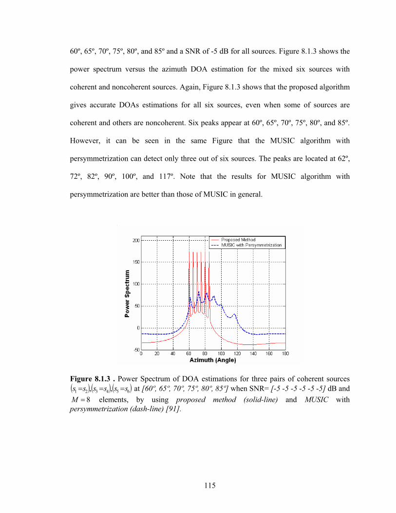
115
60º, 65º, 70º, 75º, 80º, and 85º and a SNR of -5 dB for all sources. Figure 8.1.3 shows the
power spectrum versus the azimuth DOA estimation for the mixed six sources with
coherent and noncoherent sources. Again, Figure 8.1.3 shows that the proposed algorithm
gives accurate DOAs estimations for all six sources, even when some of sources are
coherent and others are noncoherent. Six peaks appear at 60º, 65º, 70º, 75º, 80º, and 85º.
However, it can be seen in the same Figure that the MUSIC algorithm with
persymmetrization can detect only three out of six sources. The peaks are located at 62º,
72º, 82º, 90º, 100º, and 117º. Note that the results for MUSIC algorithm with
persymmetrization are better than those of MUSIC in general.
Figure 8.1.3 . Power Spectrum of DOA estimations for three pairs of coherent sources
654321 ,, ssssss at [60º, 65º, 70º, 75º, 80º, 85º] when SNR= [-5 -5 -5 -5 -5 -5] dB and
8M elements, by using proposed method (solid-line) and MUSIC with
persymmetrization (dash-line) [91].

116
Note that with the FB spatial smoothing [59] where multiple subarrays are
employed, the maximum number of degrees of freedom, i.e., the number of coherent
sources, is 2M/3 for a receiver with M number of antenna elements [92, 15 (p. 610), 93
(p. 273)]. The proposed method seems to violate this fact from the results in Figure 8.1.3
because it shows that K=6 number of sources can be resolved with M=8 elements, i.e.,
K=6 > 2M/3=5.33. But the proposed method does not use any subarrays and applies the
FB averaging over all the elements [79, 91] instead of FB spatial smoothing, which
employs many subarrays. The FB averaging method in this paper can resolve up to K<M
noncoherent sources. If the sources are coherent in pair, the FB averaging method can
resolve up to (M-1)/2 and M/2-1 coherent source pairs, for an odd and an even number of
elements M, respectively. The coherent source si and sj in pair means that they are
proportional to each other, but their arrival angles can be different from each other. For
example, the proposed method can resolve three pairs of coherent sources, such as
(s1= 1s2), (s3= 3s4), and (s5= 5s6) for M=8, where l represents the complex attenuation
of the l-th signal.
D. Simulation 4
In Figure 8.1.4 it is assumed that six uncorrelated signals are received with
azimuth DOAs at 100º, 110º, 120º, 130º, 140º, and 150º but with a realistic SNR value
such as 10 dB for all sources. This Figure shows the power spectrum versus the azimuth
angle for six uncorrelated sources with DOAs that are 10 degrees apart. It becomes clear
that the proposed algorithm gives accurate DOA estimations for all sources, and all six
peaks from the exact direction are observed. It also becomes clear that the MUSIC

117
algorithm with persymmetrization can detect only four out of six sources. As SNR
increases, MUSIC estimation is better for some sources, compared to the SNR=-5 dB
case as shown in Figure 8.1.1 the peaks of MUSIC with persymmetrization occur at 88º,
100º, 110º, 122º, 135º, and 149º.
Figure 8.1.4. Power Spectrum of DOA estimations for 6K noncoherent sources at
[100º, 110º, 120º, 130º, 140º, 150º] when SNR=[10 10 10 10 10 10] dB, and 8M
elements by using the proposed method (solid-line) and MUSIC with persymmetrization
(dash-line) [91].
E. Simulation 5
In Figure 8.1.5, it is assumeed that SNR=10 dB and source azimuth DOA
separation is 5 degrees apart such as 35º, 40º, 45º, 50º, 55º, and 60º. This Figure shows
the power spectrum versus the azimuth angle for six uncorrelated sources. Here the
proposed algorithm gives accurate DOAs estimations, and all the sources are detected,
whereas in the same Figure, the MUSIC algorithm with persymmetrization fails to detect
the six sources. Six peaks occurred at 35º, 45º, 55º, 60º, 88º, and 96º, which mean that the

118
MUSIC with persymmetrization can detect only four sources successfully at 35º, 45º, 55º,
and 60 but not the other two sources. Comparing the results in Figure 8.1.5 with those in
Figure 8.1.2, 8.1.3, it can be observed that the MUSIC with persymmetrization can detect
4 and 3 noncoherent sources at SNR=10 dB and -5 dB, respectively.
Figure 8.1.5. Power Spectrum of DOA estimations for 6K noncoherent sources at
[35º, 40º, 45º, 50º, 55º, 60º] when SNR= [10 10 10 10 10 10] dB, and 8M elements
by using the proposed method (solid-line) and MUSIC with persymmetrization (dash-
line) [91].
E. Simulation 6
For Figure 8.1.6, we assume three pairs of coherent such as 21 ss , 43 ss ,
and 65 ss . These six sources are received with the azimuth DOAs at 60º, 65º, 70º, 75º,
80º, and 85º and a SNR of 10 dB for all sources. This Figure shows the power spectrum
versus the azimuth DOA estimation for the three pair’s coherent sources. Again, Figure
8.1.6 shows that the proposed algorithm gives accurate DOAs estimations for all sources
even when the sources are coherent in pairs. The six peaks are at 60º, 65º, 70º, 75º, 80º,
and 85º. However, the same Figure shows that the MUSIC algorithm with

119
persymmetrization can detect only four out of six sources. Peaks are located at 60º, 69º,
75º, 84º, 95º, and 114º. When the results in Figure 8.1.6 are compared to 8.1.3, it can be
observed that MUSIC with persymmetrization can detect 4 and 3 sources at SNR=10 dB
and -5 dB, respectively.
Figure 8.1.6. Power Spectrum of DOA estimations for three pairs of coherent sources
654321 ,, ssssss at [60º, 65º, 70º, 75º, 80º, 85º] when SNR= [10 10 10 10 10 10] dB
and 8M elements, by using the proposed method (solid-line) and MUSIC with
persymmetrization (dash-line) [91].
8.1.4 Summary
This section proposed a method for the direction of arrival angle estimation,
employing the difference between the FB covariance matrix and the Hermition of the
backward covariance matrix. The PM was applied the method to reduce the
computational complexity, instead of taking the eigenvlue subspace schemes of eigenvlue
decomposition. Using numerical analysis, the proposed method was examined in two
situations: uncorrelated and coherent sources in pair under a correlated noise environment
whose covariance matrix is in a symmetric Toplitz form. The proposed algorithm

120
performs showed superior performance over the MUSIC algorithm with
persymmetrization and the conventional MUSIC algorithm. Moreover, the proposed
method required only the number of antenna array elements M just larger than the
number of sources K , i.e., KM , whereas the other algorithms [35-37, 90, 91]
required KM 2 . Furthermore, the proposed algorithm gave an accurate DOA
estimation even when the sources were uncorrelated, or the coherent was in pair. Testing
the proposed algorithm for SNR=10 dB and -5 dB showed that it performed well, even
when the SNR was -5 dB, and the DOA separation was as small as 5 degrees.
8.2 1-D DOA Estimation for Coherent Sources with Spatial Smoothing
This section presents 1-D DOA estimation for uncorrelated sources or coherent
sources in pairs under unknown correlated noise environment in symmetric Toeplitz
form. Here the proposed method is extended to when all sources are coherent instead of
coherent in pairs by employing forward-backward spatial smoothing.
8.2.1 System Model
In equation (8.1.1) in previous section, the signal covariance matrix
)()( tstsER HS is diagonal and nonsingular when the incident signals are uncorrelated.
In this situation, H
s AAR has a rank of K, which means the DOAs can be resolved for all
incident sources when KM by using the popular classical subspace MUSIC and
ESPRIT algorithms [14, 9]. However, these algorithms give poor performance in a multi-
path environment because the signals become coherent, and the covariance noise matrix
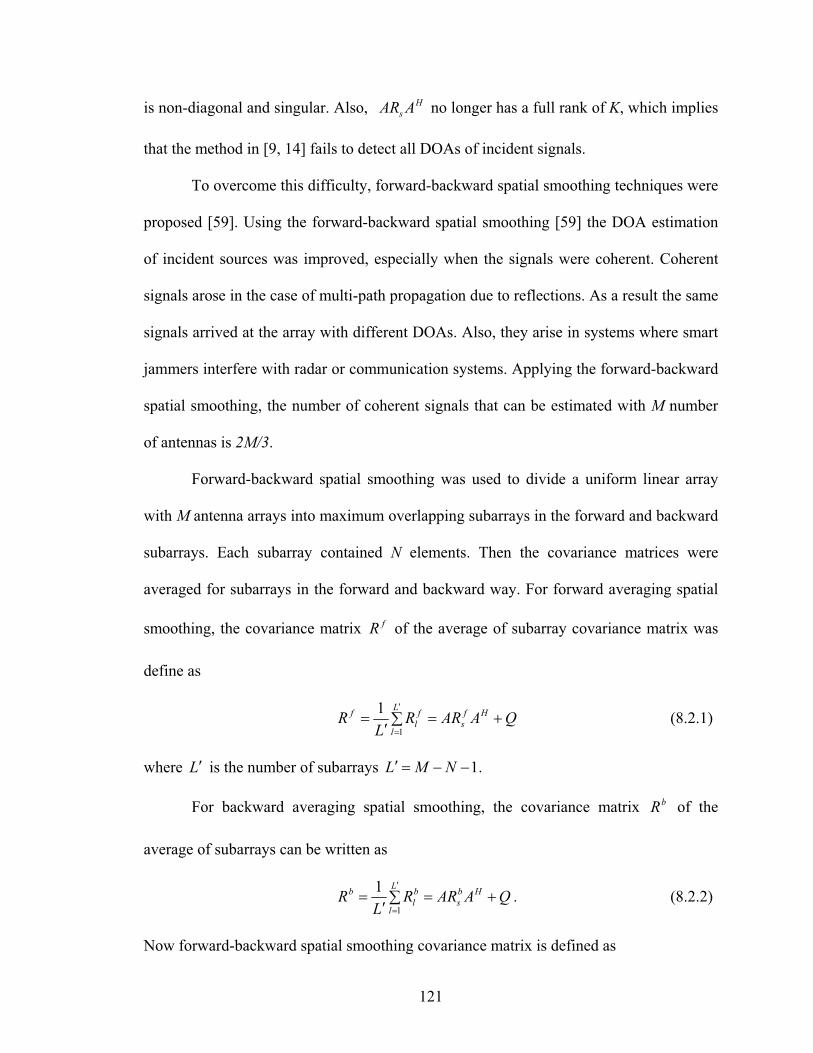
121
is non-diagonal and singular. Also, H
s AAR no longer has a full rank of K, which implies
that the method in [9, 14] fails to detect all DOAs of incident signals.
To overcome this difficulty, forward-backward spatial smoothing techniques were
proposed [59]. Using the forward-backward spatial smoothing [59] the DOA estimation
of incident sources was improved, especially when the signals were coherent. Coherent
signals arose in the case of multi-path propagation due to reflections. As a result the same
signals arrived at the array with different DOAs. Also, they arise in systems where smart
jammers interfere with radar or communication systems. Applying the forward-backward
spatial smoothing, the number of coherent signals that can be estimated with M number
of antennas is 2M/3.
Forward-backward spatial smoothing was used to divide a uniform linear array
with M antenna arrays into maximum overlapping subarrays in the forward and backward
subarrays. Each subarray contained N elements. Then the covariance matrices were
averaged for subarrays in the forward and backward way. For forward averaging spatial
smoothing, the covariance matrix fR of the average of subarray covariance matrix was
define as
QAARRL
R Hf
s
L
l
f
l
f
1
1 (8.2.1)
where L is the number of subarrays .1NML
For backward averaging spatial smoothing, the covariance matrix bR of the
average of subarrays can be written as
QAARRL
R HL
l
b
s
b
l
b
1
1. (8.2.2)
Now forward-backward spatial smoothing covariance matrix is defined as

122
2
bf RRR . (8.2.3)
Using equation (8.1.3) the forward-backward spatial smoothing in equation (8.2.3) can be
rewritten as
JJRRR ff
2
1. (8.2.4)
The proposed method, we are employing the forward-backward spatial smoothing
for the covariance matrix of the observation data. This scheme can eliminate the noise
effect on the array structure by taking the difference R between the forward-backward
spatial smoothing R and the Hermition of the backward covariance matrix
JRJJJRTfHf as
JRJRRT
fˆˆˆ JRJJRJRT
fff ˆˆˆ2
1. (8.2.5)
Substituting equation (8.1.1) into equation (8.2.5) yields
JJQJAARJJJQJARJAQAARR TTHf
s
Hf
s
Hf
s2
1. (8.2.6)
Equation (8.1.7) is valid when either the unknown noise covariance matrix Q is in
the form of complex or real symmetric Toeplitz. Note that the method in [37], which
employs JRJRR , can only eliminate Q completely if Q is a real symmetric
Toeplitz because in this case JJQQ . However, if the unknown covariance noise
matrix is in a complex symmetric Toeplitz, the method fails to eliminate Q, because in
this situation JJQQ .
Substituting equation (8.1.7) into equation (8.2.6)

123
JAARJJARJAAAR
QJAARJQJARJAQAARR
THf
S
Hf
S
Hf
S
THf
s
Hf
s
Hf
s
2
1
2
1
(8.2.7)
Note that the covariance matrix Q of the unknown noise is completely removed in
equation (8.2.7), since Q either is complex or real. Then, the DOA for coherent sources
can be found by applying the same equations (8.1.9) through (8.1.18), using the different
R in equation (8.2.7) instead of equation (8.1.8).
8.2.2 Numerical Analysis
In this section, the performance of the proposed method is compared to the
forward-backward spatial smoothing algorithm in [59]. Performance is verified through a
numerical analysis for coherent sources under the unknown correlated noise of a real and
complex symmetric Toeplitz covariance matrix. K=5 and K=3 considered as coherent
sources of different SNR values and different DOAs, and a ULA consisting of eight
sensors 8M with spacing equal to a half wavelength. Two cases of unknown noise
covariance matrix are assumed: Case (1), a real symmetric Toeplitz form whose top row
is 7529.08004.8587.9084.9555.1 and Case (2), a complex symmetric
Toelpitz with top row is iiiii 35.055.48.65.45.75.32.85.035.09.1 .
The diagonal elements have a correlation coefficient equal to one which is stronger than
those of the off-diagonal elements, and the correlation coefficients are getting smaller as
they are getting farther away from the diagonal.
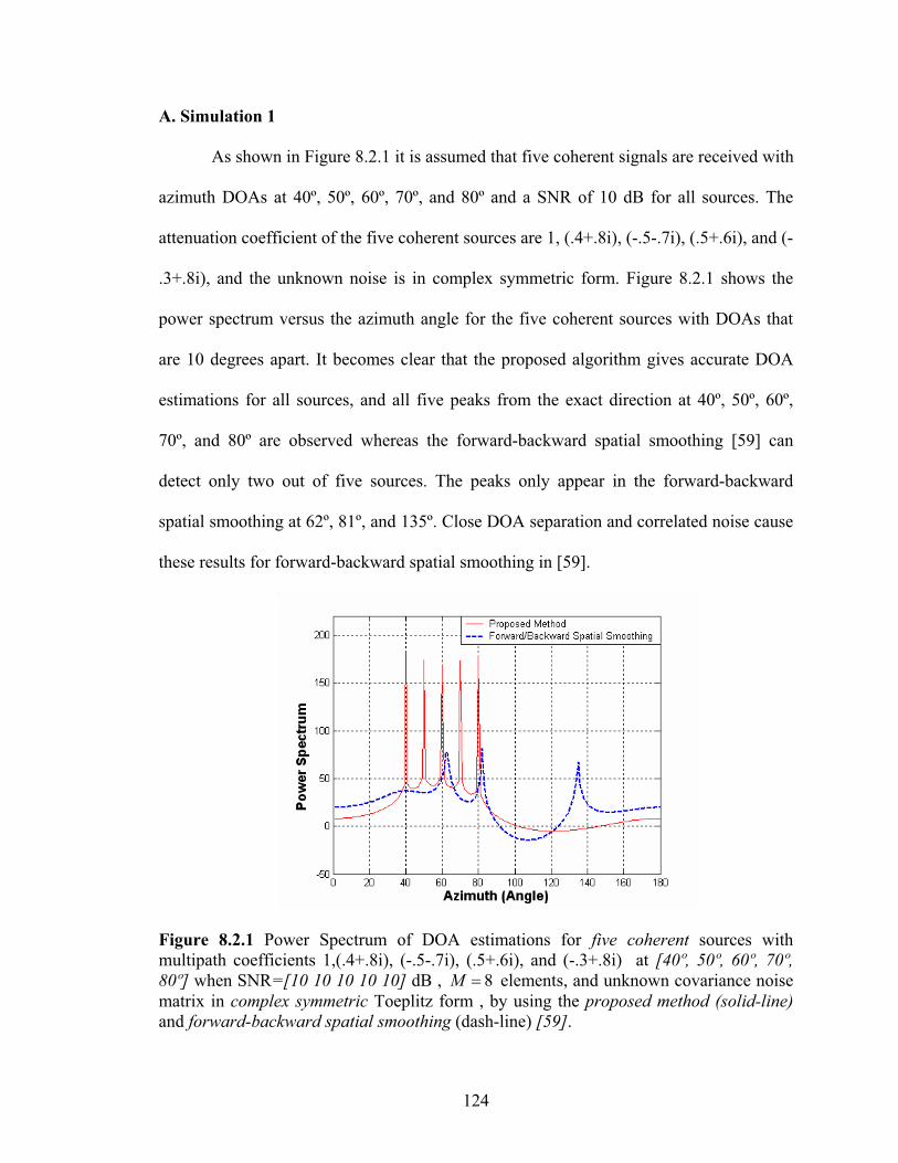
124
A. Simulation 1
As shown in Figure 8.2.1 it is assumed that five coherent signals are received with
azimuth DOAs at 40º, 50º, 60º, 70º, and 80º and a SNR of 10 dB for all sources. The
attenuation coefficient of the five coherent sources are 1, (.4+.8i), (-.5-.7i), (.5+.6i), and (-
.3+.8i), and the unknown noise is in complex symmetric form. Figure 8.2.1 shows the
power spectrum versus the azimuth angle for the five coherent sources with DOAs that
are 10 degrees apart. It becomes clear that the proposed algorithm gives accurate DOA
estimations for all sources, and all five peaks from the exact direction at 40º, 50º, 60º,
70º, and 80º are observed whereas the forward-backward spatial smoothing [59] can
detect only two out of five sources. The peaks only appear in the forward-backward
spatial smoothing at 62º, 81º, and 135º. Close DOA separation and correlated noise cause
these results for forward-backward spatial smoothing in [59].
Figure 8.2.1 Power Spectrum of DOA estimations for five coherent sources with
multipath coefficients 1,(.4+.8i), (-.5-.7i), (.5+.6i), and (-.3+.8i) at [40º, 50º, 60º, 70º,
80º] when SNR=[10 10 10 10 10] dB , 8M elements, and unknown covariance noise
matrix in complex symmetric Toeplitz form , by using the proposed method (solid-line)
and forward-backward spatial smoothing (dash-line) [59].

125
B. The Simulation 2:
In Figure 8.2.2 it is assumed that the parameters is the same as the ones used in
Figure 8.2.1 but the unknown noise covariance matrix is changed to be in a real
symmetric Toeplitz form. Figure 8.2.2 shows the power spectrum versus the azimuth
angle for the five uncorrelated sources. Here the proposed algorithm gives accurate
DOAs estimations, and all the sources are detected, whereas in the same Figure the
forward-backward spatial smoothing fails to detect the five sources. Five peaks occurred
at 39º, 61º, 79º, 91º, and 120º, which mean that the MUSIC can detect only three sources
successfully at 39º, 61º, and 79º, but the other two that were detected incorrectly. When
the results in Figure 8.2.1 compared with those in Figure 8.2.2, it can be observed that the
forward-backward spatial smoothing can detect more sources in Figure 8.2.1, which
means that when the unknown noise is in complex symmetric form the performance
becomes worse, compared with the real symmetric Toeplitz unknown noise
environments.
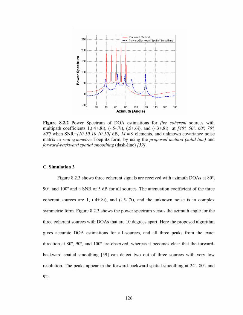
126
Figure 8.2.2 Power Spectrum of DOA estimations for five coherent sources with
multipath coefficients 1,(.4+.8i), (-.5-.7i), (.5+.6i), and (-.3+.8i) at [40º, 50º, 60º, 70º,
80º] when SNR=[10 10 10 10 10] dB, 8M elements, and unknown covariance noise
matrix in real symmetric Toeplitz form, by using the proposed method (solid-line) and
forward-backward spatial smoothing (dash-line) [59].
C. Simulation 3
Figure 8.2.3 shows three coherent signals are received with azimuth DOAs at 80º,
90º, and 100º and a SNR of 5 dB for all sources. The attenuation coefficient of the three
coherent sources are 1, (.4+.8i), and (-.5-.7i), and the unknown noise is in complex
symmetric form. Figure 8.2.3 shows the power spectrum versus the azimuth angle for the
three coherent sources with DOAs that are 10 degrees apart. Here the proposed algorithm
gives accurate DOA estimations for all sources, and all three peaks from the exact
direction at 80º, 90º, and 100º are observed, whereas it becomes clear that the forward-
backward spatial smoothing [59] can detect two out of three sources with very low
resolution. The peaks appear in the forward-backward spatial smoothing at 24º, 80º, and
92º.

127
Figure 8.2.3 Power Spectrum of DOA estimations for three coherent sources with
multipath coefficients 1, (.4+.8i), and (-.5-.7i), [80º, 90º, 100º] when SNR=[5 5 5]dB,
8M elements, and unknown covariance noise matrix in complex symmetric Toeplitz
form, by using the proposed method (solid-line) and forward-backward spatial
smoothing (dash-line) [59].
F. Simulation 4
In Figure 8.2.4, it is assumed the same parameters as the ones used in Figure
8.2.3, but the unknown noise covariance matrix is changed to be in a real symmetric
Toeplitz. Figure 8.2.4 show the power spectrum versus the azimuth angle for the three
uncorrelated sources. Here the proposed algorithm gives accurate DOAs estimations with
very high resolution, and all the sources are detected, whereas in the same Figure the
forward-backward spatial smoothing detects the sources with very low resolution. Again
when the results in Figure 8.2.3 compared with those in Figure 8.2.4, it can be observed
that the forward-backward spatial smoothing can give a better performance when the
unknown covariance noise matrix is a real symmetric Toeplitz form.

128
Figure 8.2.4 Power Spectrum of DOA estimations for three coherent sources with
multipath coefficients 1, (.4+.8i), and (-.5-.7i), [80º, 90º, 100º] when SNR=[5 5 5]dB,
8M elements, and unknown covariance noise matrix in real symmetric Toeplitz form,
by using the proposed method (solid-line) and forward-backward spatial smoothing
(dash-line) [59].
F. Simulation 5
In Figure 8.2.5, it is assumed that the SNR=5 dB, and three coherent sources are
received with azimuth DOA separation of 5 degrees apart such as 70º, 75º, and 80º. The
attenuation coefficient of the three coherent sources are 1, (.4+.8i), and (-.5-.7i), and the
unknown noise is in a complex symmetric form. Figure 8.2.5 shows the power spectrum
versus the azimuth angle for the three coherent sources. Here the proposed algorithm
gives accurate DOA estimations for all sources, and all the sources are detected even if
the DOAs of the sources are separated by only 5º, whereas it becomes clear that the
forward-backward spatial smoothing [59] can detect only two out of three sources with
less resolution, compared to Figure 8.2.3. The peaks appear in the forward-backward
spatial smoothing at 23º, 71º, and 78º.
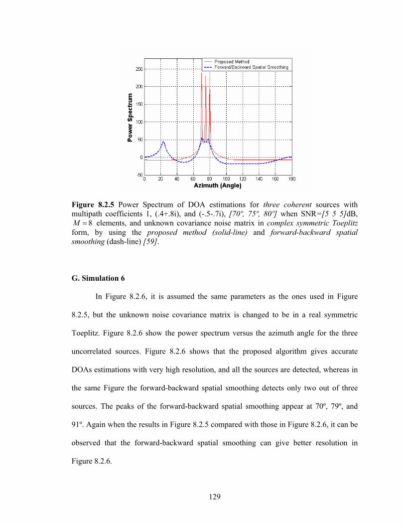
129
Figure 8.2.5 Power Spectrum of DOA estimations for three coherent sources with
multipath coefficients 1, (.4+.8i), and (-.5-.7i), [70º, 75º, 80º] when SNR=[5 5 5]dB,
8M elements, and unknown covariance noise matrix in complex symmetric Toeplitz
form, by using the proposed method (solid-line) and forward-backward spatial
smoothing (dash-line) [59].
G. Simulation 6
In Figure 8.2.6, it is assumed the same parameters as the ones used in Figure
8.2.5, but the unknown noise covariance matrix is changed to be in a real symmetric
Toeplitz. Figure 8.2.6 show the power spectrum versus the azimuth angle for the three
uncorrelated sources. Figure 8.2.6 shows that the proposed algorithm gives accurate
DOAs estimations with very high resolution, and all the sources are detected, whereas in
the same Figure the forward-backward spatial smoothing detects only two out of three
sources. The peaks of the forward-backward spatial smoothing appear at 70º, 79º, and
91º. Again when the results in Figure 8.2.5 compared with those in Figure 8.2.6, it can be
observed that the forward-backward spatial smoothing can give better resolution in
Figure 8.2.6.

130
Figure 8.2.6 Power Spectrum of DOA estimations for three coherent sources with
multipath coefficients 1, (.4+.8i), and (-.5-.7i), [70º, 75º, 80º] when SNR=[5 5 5]dB,
8M elements, and unknown covariance noise matrix in real symmetric Toeplitz form,
by using the proposed method (solid-line) and forward-backward spatial smoothing
(dash-line) [59].
8.2.3 Summary
This section proposed a method for the direction of arrival angle estimation,
employing the difference between the forward-backward spatial smoothing covariance
matrix and the Hermition of the backward smoothing covariance matrix. The PM was
then applied to the method to reduce the computational complexity, instead of taking the
eigenvalue subspace schemes of eigenvalue decomposition. Through the numerical
analysis, the proposed method was examined when the incident signals are coherent
under a correlated noise environment whose covariance matrix is in a real or complex
symmetric Toeplitz form. The proposed algorithm showed superior performance over the
forward-backward spatial smoothing. Moreover, the proposed method requires only the
number of antenna KM .

131
8.3 2-D DOA Estimation with Forward-Backward Averaging
This section introduces a proposed method which employs PM for 1-D DOA
estimation under unknown correlated noise environment. Here the proposed method is
applied in the situation, when the incident sources are uncorrelated or coherent in pairs.
Also, the proposed method is extended the 1-D DOA estimation to 2-D DOA estimation
for the same environments. The numerical results verify that the proposed method
performs successfully under the environment where the method in [37] fails, and
furthermore gives better performance and less computation than the conventional
MUSIC.
8.3.1 Introduction
Two-dimensional (2-D) DOA estimation, i.e., azimuth and elevation , has
played an important role in array signal processing in many areas such as Radar, sonar,
and mobile communication systems. Estimation of 2-D DOA azimuth and elevation
angles will give more information about the location of the incident sources. This will
improve the performance of the system. In the proposed algorithm, we use L-shape array
in x-z plane to achieve the 2-D DOA estimation. Also, the case of unknown spatially
colored noise environments is considered in addition to coherent sources in pairs or
noncoherent sources. Furthermore, this chapter focuses on the unknown colored noise
with its covariance matrix in the symmetric Toeplitz form as [37, 86-90]. The proposed
method can be applicable to the 2-D DOA estimations whereas the method in [37]
studied only for the 1-D DOA estimation problem and noncoherent sources.

132
8.3.2 System Model
Figure 8.3.1 shows the L-shape array configuration which uses x-z plane instead
of x-y. Each linear array consists of N elements. The element placed at the origin is
common for referencing purpose. Let T
N tztztzt )](),...,(),([)(Z 21 be the (N×1) received
signal vector at the uniform linear array (ULA) elements in the z axis where superscript T
denotes the transpose, and let T
N txtxtxt )](),...,(),([)(X 21 be the (N×1) received signal
vector at the ULA elements in the x axis. Suppose that there are K narrowband sources
where the k -th source has an elevation angle k and an azimuth angle k , k=1, …, K.
k
k1
1
x
z
y
Kk ,...,1)(tsk
.
..
...
reference
N
N
0
Figure 8.3.1. Two orthogonal uniform linear arrays in x-z plane used for joint elevation
and azimuth ),( DOA estimation by the proposed method.
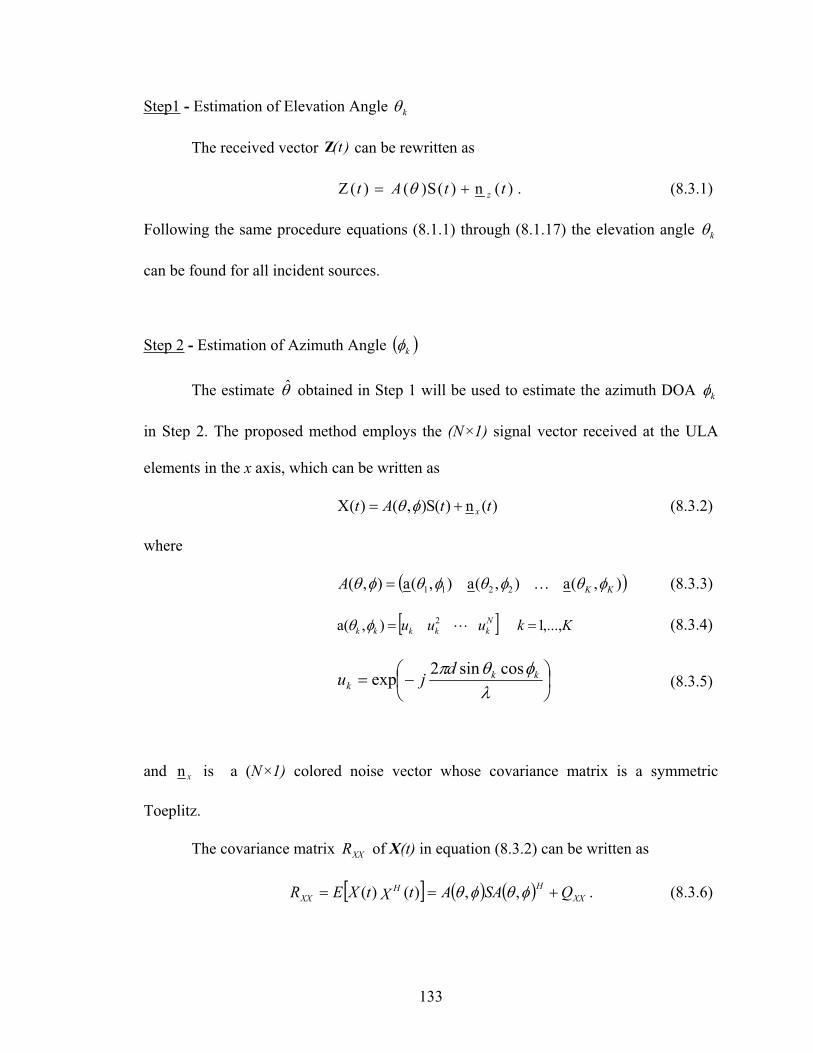
133
Step1 - Estimation of Elevation Angle k
The received vector )t(Z can be rewritten as
)(n)(S)()(Z ttAt z . (8.3.1)
Following the same procedure equations (8.1.1) through (8.1.17) the elevation angle k
can be found for all incident sources.
Step 2 - Estimation of Azimuth Angle k
The estimate ˆ obtained in Step 1 will be used to estimate the azimuth DOA k
in Step 2. The proposed method employs the (N×1) signal vector received at the ULA
elements in the x axis, which can be written as
)(n)(S),()(X ttAt x (8.3.2)
where
),(a),(a),(a),( 2211 KKA (8.3.3)
Kkuuu N
kkkkk ,...,1),(a 2 (8.3.4)
kkk
dju
cossin2exp (8.3.5)
and xn is a (N×1) colored noise vector whose covariance matrix is a symmetric
Toeplitz.
The covariance matrix XXR of X(t) in equation (8.3.2) can be written as
XX
HHXX QSAAtXtXER ,,)()( . (8.3.6)
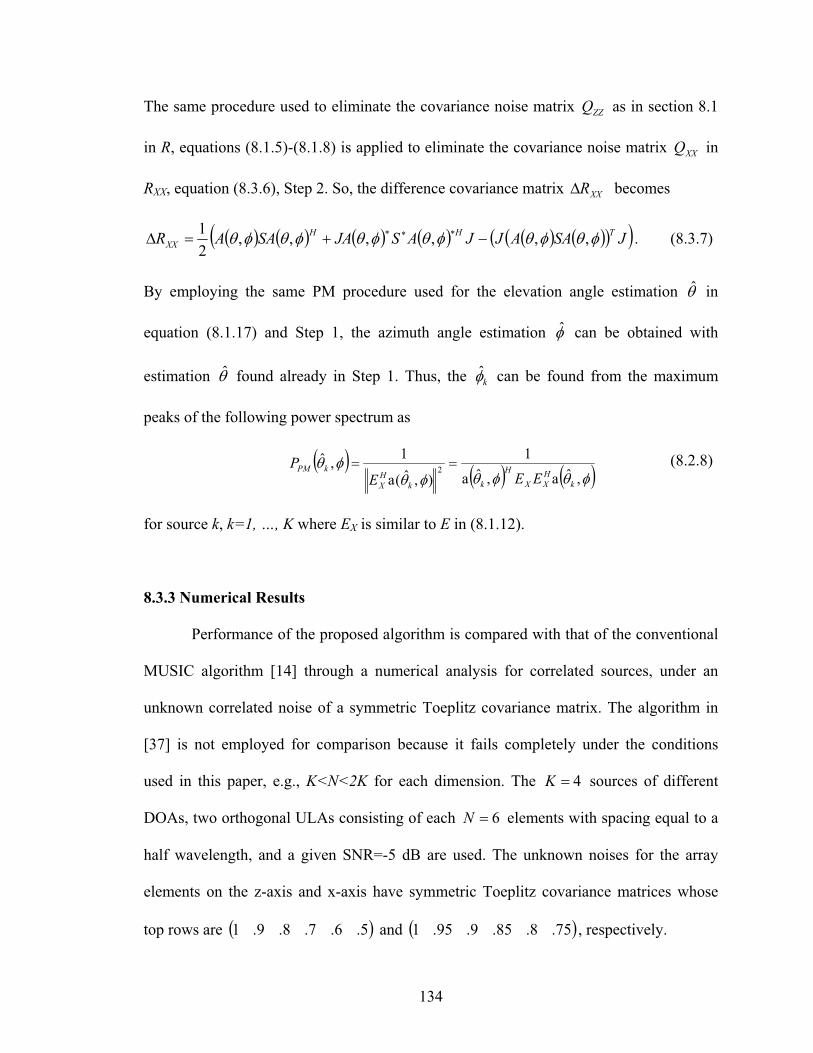
134
The same procedure used to eliminate the covariance noise matrix ZZQ as in section 8.1
in R, equations (8.1.5)-(8.1.8) is applied to eliminate the covariance noise matrix XXQ in
RXX, equation (8.3.6), Step 2. So, the difference covariance matrix XXR becomes
JSAAJJASJASAARTHH
XX ,,,,,,2
1. (8.3.7)
By employing the same PM procedure used for the elevation angle estimation ˆ in
equation (8.1.17) and Step 1, the azimuth angle estimation ˆ can be obtained with
estimation ˆ found already in Step 1. Thus, the kˆ can be found from the maximum
peaks of the following power spectrum as
,ˆa,ˆa
1
),ˆ(a
1,ˆ
2
k
H
XX
H
kk
H
X
kPM
EEE
P (8.2.8)
for source k, k=1, …, K where EX is similar to E in (8.1.12).
8.3.3 Numerical Results
Performance of the proposed algorithm is compared with that of the conventional
MUSIC algorithm [14] through a numerical analysis for correlated sources, under an
unknown correlated noise of a symmetric Toeplitz covariance matrix. The algorithm in
[37] is not employed for comparison because it fails completely under the conditions
used in this paper, e.g., K<N<2K for each dimension. The 4K sources of different
DOAs, two orthogonal ULAs consisting of each 6N elements with spacing equal to a
half wavelength, and a given SNR=-5 dB are used. The unknown noises for the array
elements on the z-axis and x-axis have symmetric Toeplitz covariance matrices whose
top rows are 5.6.7.8.9.1 and 75.8.85.9.95.1 , respectively.
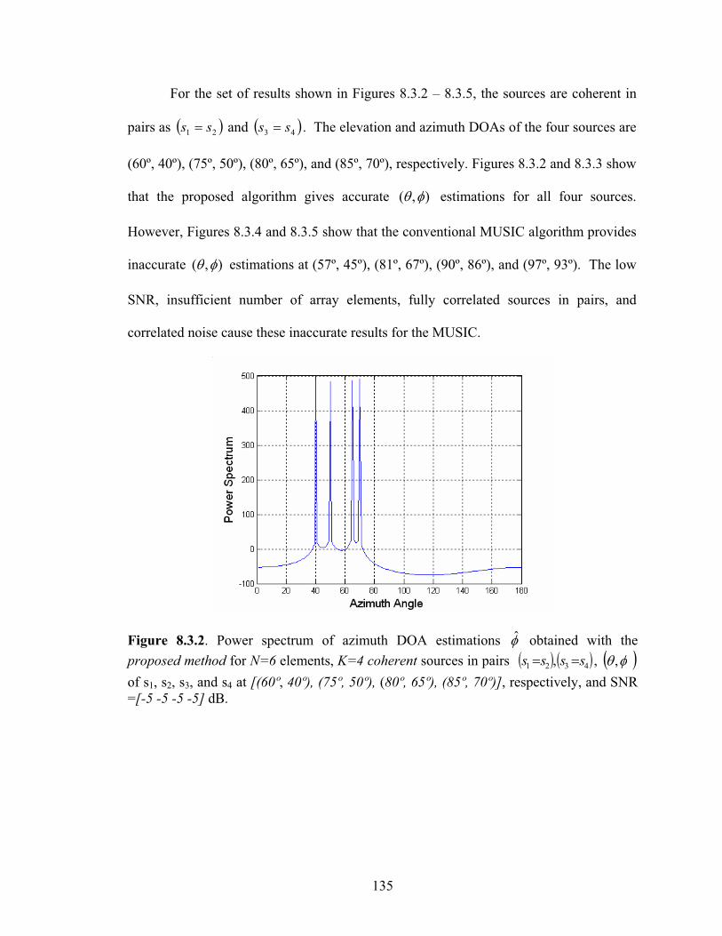
135
For the set of results shown in Figures 8.3.2 – 8.3.5, the sources are coherent in
pairs as 21 ss and 43 ss . The elevation and azimuth DOAs of the four sources are
(60º, 40º), (75º, 50º), (80º, 65º), and (85º, 70º), respectively. Figures 8.3.2 and 8.3.3 show
that the proposed algorithm gives accurate ),( estimations for all four sources.
However, Figures 8.3.4 and 8.3.5 show that the conventional MUSIC algorithm provides
inaccurate ),( estimations at (57º, 45º), (81º, 67º), (90º, 86º), and (97º, 93º). The low
SNR, insufficient number of array elements, fully correlated sources in pairs, and
correlated noise cause these inaccurate results for the MUSIC.
Figure 8.3.2. Power spectrum of azimuth DOA estimations ˆ obtained with the
proposed method for N=6 elements, K=4 coherent sources in pairs 4321 , ssss , ,
of s1, s2, s3, and s4 at [(60º, 40º), (75º, 50º), (80º, 65º), (85º, 70º)], respectively, and SNR
=[-5 -5 -5 -5] dB.
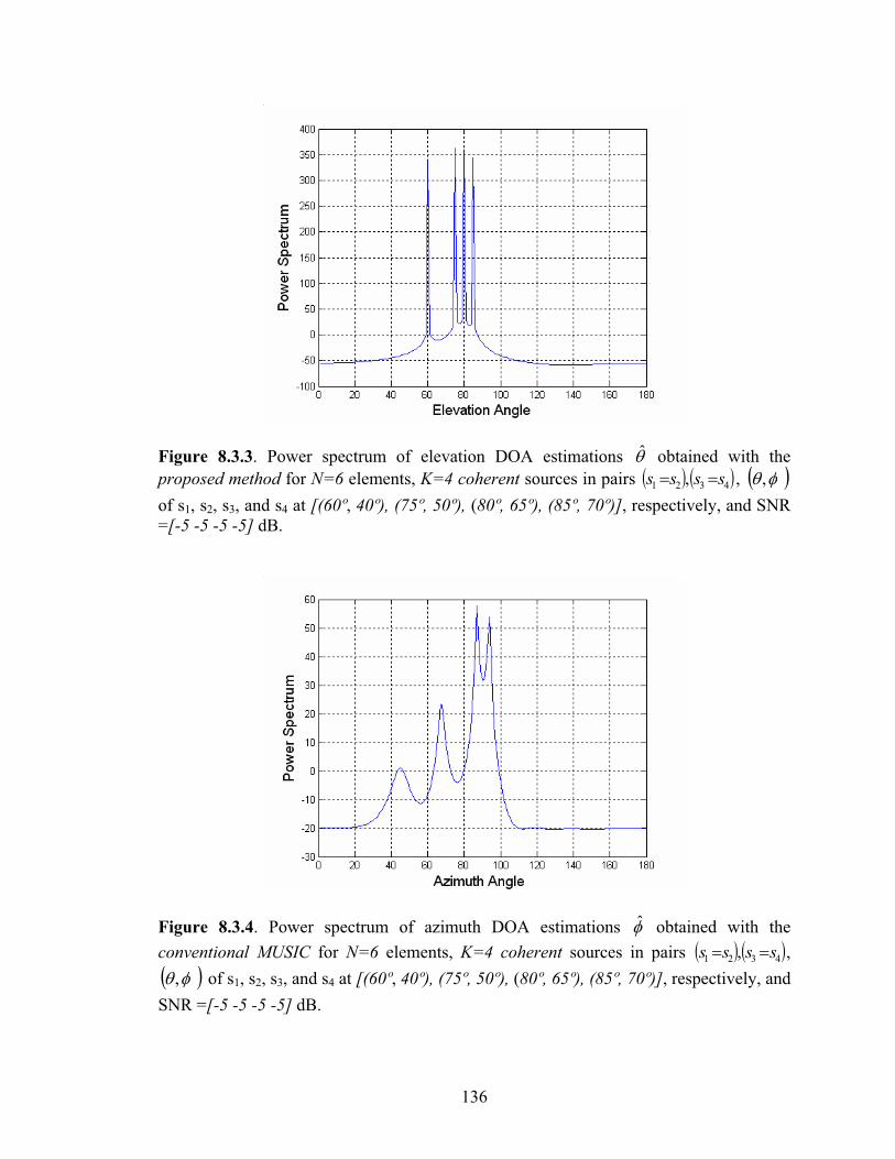
136
Figure 8.3.3. Power spectrum of elevation DOA estimations ˆ obtained with the
proposed method for N=6 elements, K=4 coherent sources in pairs 4321 , ssss , ,
of s1, s2, s3, and s4 at [(60º, 40º), (75º, 50º), (80º, 65º), (85º, 70º)], respectively, and SNR
=[-5 -5 -5 -5] dB.
Figure 8.3.4. Power spectrum of azimuth DOA estimations ˆ obtained with the
conventional MUSIC for N=6 elements, K=4 coherent sources in pairs 4321 , ssss ,
, of s1, s2, s3, and s4 at [(60º, 40º), (75º, 50º), (80º, 65º), (85º, 70º)], respectively, and
SNR =[-5 -5 -5 -5] dB.
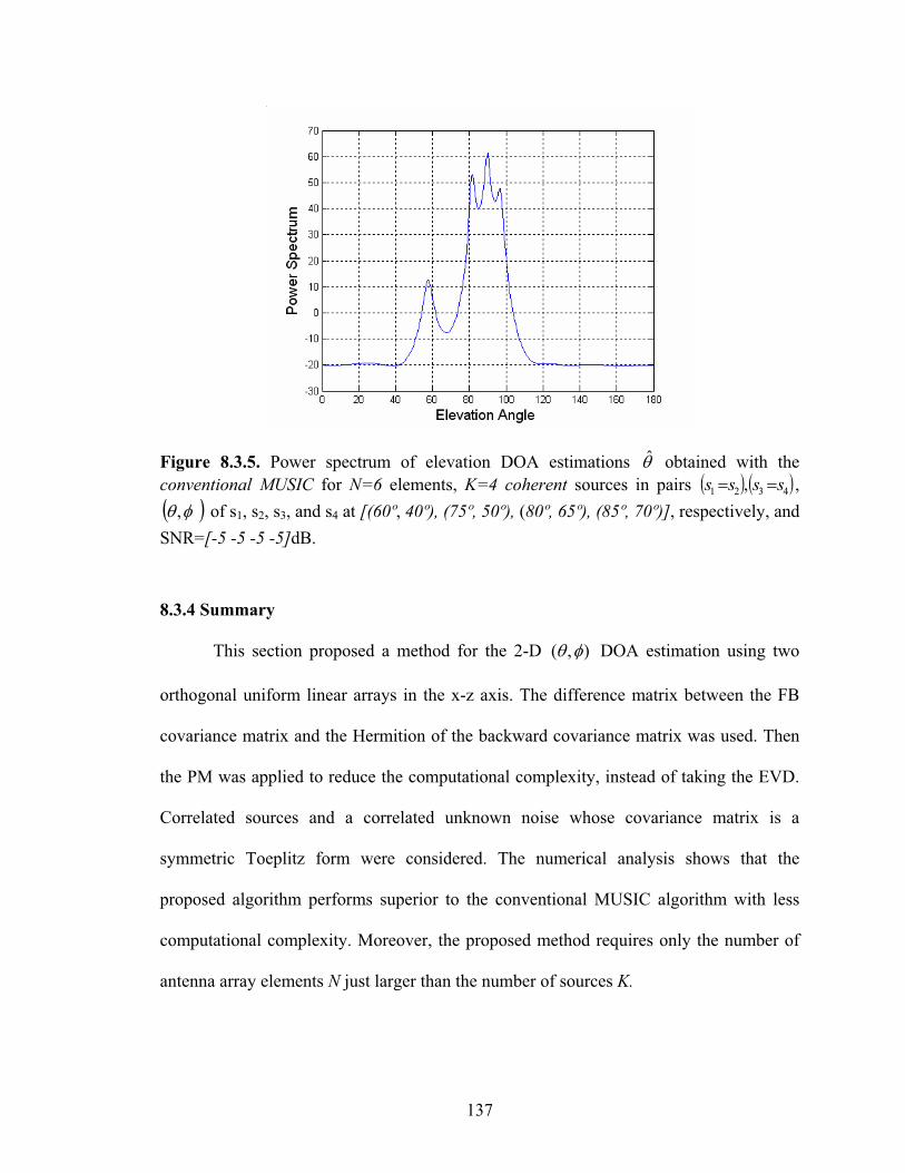
137
Figure 8.3.5. Power spectrum of elevation DOA estimations ˆ obtained with the
conventional MUSIC for N=6 elements, K=4 coherent sources in pairs 4321 , ssss ,
, of s1, s2, s3, and s4 at [(60º, 40º), (75º, 50º), (80º, 65º), (85º, 70º)], respectively, and
SNR=[-5 -5 -5 -5]dB.
8.3.4 Summary
This section proposed a method for the 2-D ),( DOA estimation using two
orthogonal uniform linear arrays in the x-z axis. The difference matrix between the FB
covariance matrix and the Hermition of the backward covariance matrix was used. Then
the PM was applied to reduce the computational complexity, instead of taking the EVD.
Correlated sources and a correlated unknown noise whose covariance matrix is a
symmetric Toeplitz form were considered. The numerical analysis shows that the
proposed algorithm performs superior to the conventional MUSIC algorithm with less
computational complexity. Moreover, the proposed method requires only the number of
antenna array elements N just larger than the number of sources K.

138
CHAPTER 9
CONCLUSIONS AND FUTURE WORK
9.1 Conclusions
This dissertation introduced and proposed several methods that would be
beneficial to solve the problem of signal parameter estimation DOA for 1-D and 2-D
cases. Chapter 1 provided a brief introduction of the array signal processing area,
background and motivation, a list of main contributions of the dissertation, and an
outline. Chapter 2 provided the signal model and an overview about some DOA
estimation schemes, conventional beamforming, Capon’s method, the MUSIC algorithm,
and the ESPRIT algorithm. Chapter 3 proposed a scheme for 1-D and 2-D DOA
estimations that does not require any pair matching and gives good performance under
low SNR values. Chapter 4 introduced a 2-D DOA estimation called the PMV-ESPRIT
algorithm, which does not require any EVD or SVD and can reduce the complexity. Also,
the PMV-ESPRIT algorithm does not need the pair matching between the azimuth and
elevation angles. Hence, it will be more appropriate for real-time implementation, than
V-ESPIRIT and the PM with doublet configuration.
In Chapters 5 and 6, antenna array configurations were proposed for the 2-D
azimuth and elevation angle estimation problem and compared with the parallel-shape
configuration. The proposed methods employ a PM which does not require any EVD or
SVD but only a linear operation. The proposed 2-D DOA estimation schemes show
significant improvement over the existing schemes. The proposed schemes do not have
any failure of estimation, especially in the regions that would be practical in mobile

139
communications, whereas other existing schemes can have 50 percent. In addition, no
pair matching for the 2-D DOA estimation problems is required.
Chapter 7, we provided a scheme for 1-D DOA estimation from multiple
incident signals under an unknown spatially non-stationary white noise environment, i.e.,
with a diagonal covariance matrix whose diagonal elements have unequal noise power.
Numerical results show that the proposed algorithm gives accurate estimation even if the
sources are uncorrelated or coherent in pairs.
Chapter 8 presented the proposed method for the 1-D and 2-D DOA estimations
without any EVD or SVD, this reducing computational complexity. It is assumed that the
sources are uncorrelated or coherent sources under a correlated noise environment whose
covariance matrix is in a symmetric Toeplitz form. It was observed that the proposed
algorithm performs superior to the MUSIC algorithm with persymmetrization and the
conventional MUSIC algorithm. Moreover, the proposed method requires only the
number of antenna array elements M just larger than the number of sources K , i.e.,
KM , whereas the other algorithms [35-37, 90] require that KM 2 .
9.2 Future Work
The work in this dissertation represents a significant advancement for array signal
processing in many areas such as radar, sonar, radio astronomy, seismic data processing,
and mobile communication systems. However, it is by no means the final definitive work
on any subject. A number of future projects that would build on this thesis include the
following:
140
1. Extension of C-SPRIT algorithm for other modulation schemes such as
Quadrature Phase-Shift Keying (QPSK) and Quadrature Amplitude Modulation
(QAM).
2. DOA estimation for wideband signals.
3. Extinction of DOA estimation schemes for distributed sources.
4. Angle and frequency estimation for incident sources under wideband and
narrowband signals for point and distributed sources.
5. DOA estimation in uplink and downlink beamforming for CDMA systems.
6. Double directional finding (angle of departure and angle of arrival) for MIMO
(multiple-input-multiple output) channel.

141
REFERENCES

142
LIST OF REFERENCES
1. P. E. Green, E. J. Kelly and M. J. Levin, “A comparison of seismic array proceeding
methods,” Geophy. J. Royal. Astron. Soc., Vol. 11, pp. 67-84, 1996.
2. W. Vanderkulk, “Optimum processing of acoustic arrays,” J. Br. Inst. Radio Eng.,
Vol. 34, pp. 285-292, 1963.
3. J. W. R. Griffiths and J.E. Hudson, “An introduction to adaptive processing in a
passive sonar system,” Aspects of Signal Processing, Pt.1, NATO Advanced Study
Institute Series, D. Reidel Publishing Co., Dordrecht, Holland, 1977.
4. L. E. Brennan and I.S. Reed, “Theory of adaptive radar,” IEEE Trans. Aerospace
and Electronics Systems, AES-9 pp. 237-252, November 1973.
5. J. H. Winters, “Optimum combining in digital mobile radio with cochannel
interference,” IEEE J. Select. Area Commun, Vol. COM-35, pp. 1222-1230, 1987.
6. B. Suard , A. F. Naguib, G. Xu, and A. Paulraj, “ Performance of CDMA mobile
communication systems using antenna arrays,” IEEE Int. Conf. Acoustics, Speech ,
and Signal Processing (ICASSP), Minneapolis, MN, pp. 153-156, 1993
7. A. Flieller, P. Larzabal, and H. Clergeot, “A placations of high resolution array
processing techniques for mobile communication system,” in Proc. IEEE Intelligent
Vehicles Symp., Paris, France, pp. 606-611, 1994
8. R. O. Schmidt, “A signal subspace approach to multiple emitter location and
spectral estimation,” Ph.D. dissertation, Dept. Elect. Eng., Stanford Univ., Stanford,
CA, November 1981.
9. R. O. Schmidt, “Multiple emitter location and signal parameter estimation,” IEEE
Trans. Antennas Propagation, Vol. 34, pp. 276-280, March 1986.
10. G. Bienvenu and L. Kopp, “Principle de la gonionmetrie passive adaptive,”
Proc.7’eme Colloque GRESIT (Nice, France), pp. 106/1 – 106/10, 1979.
11. R. O. Schmidt, “Multiple emitter location and signal parameter estimation,” Proc.
RADC Spectrum Estimation Workshop (Rome, NY), pp. 243-258, 1979.
12. R. H. Roy, “ESPRIT-Estimation of signal parameters via rotational invariance
techniques,” Ph.D. dissertation, Dept. Elect. Eng., Stanford Univ., 1987.
13. A. Swindlehurst and T. Kailath, “Azimuth/elevation direction finding using regular
array geometries,” IEEE Trans. on Aerospace and Electronic Systems, Vol. 29,
No.1, pp. 145-155, January 1993.
143
14. R. Roy, A. Paulraj, and T. Kailath, “Estimation of signal parameters via rotational
invariance techniques – ESPRIT,” in Proc. IEEE ICASSP, Vol. 4, Tokyo, Japan, pp.
2495-2498, 1986.
15. R. Roy and T. Kailath, “ESPRIT –Estimation of signal parameters via rotational
invariance techniques,” Optical Engineering, Vol. 29, No .4, pp. 296-313, April
1990.
16. R. Roy, A. Paulraj, and T. Kailath, “ESPRIT-A subspace rotational approach to
estimation of parameters of cissoids in noise,” IEEE Trans. Acoustics, Speech,
Signal Processing, Vol. 34, No. 4, pp. 1340-1342, October 1986.
17. A. Paulraj, R. Roy, and T. Kailath, “Estimation of signal parameters via rotations
invariance techniques –ESPRIT,” in Proc. Nineteenth Asilomer Conf. Circuits, Syst.,
Comput. (Asilomar, CA), November 1985.
18. A. Paulraj, R. Roy, and T. Kailath, “A subspace rotation approach to signal
parameters estimation,” in Proc. IEEE, pp. 1044-1445, July 1986.
19. G. Xu, S. Silverstein, R. Roy, and T. Kailath, “Beamspace ESPRIT,” IEEE Trans.
Signal Processing, Vol. 42, pp. 349-356, February 1994.
20. P. F. Krekel and E. F. Deprettere, “A two-diminsional version of the matrix pencil
method to solve the DOA problem,” European Conference on Circuit Theory and
Design, pp. 435-439, 1989.
21. Q. Yin, R.W. Newcomb and Li-He Zou, “ Estimation 2-D angles of arrival via
parallel linear array,” ICASSP-89, 1989 International Conference on Acoustics,
Speech, and Signal Processing , Vol. 4, pp. 2803-2806, 1989.
22. F. A. Sakarya and M. W. Hayes, “Estimation 2-D DOA using nonlinear array
configurations,” IEEE Trans. Signal Processing, Vol. 43, pp. 2212-2216, September
1995.
23. A. Swindlehurst and T. Kailath, “2-D parameter estimation using arrays with
multidimensional invariance structure,” 23ACSSC, Vol. 29, pp. 950-953, December
1989.
24. Y. Wu, G. Liao, and H. C. So, “A fast algorithm for 2-D direction-of-arrival
estimation,” Signal Processing, Vol. 83, pp. 1827-1831, 2003.
25. J. Fernandez del Rio and M. Catedra-Peraz, “The matrix pencil method for two-
dimensional direction of arrival estimation employing L-shaped array,” IEEE Trans.
Antennas Propagation, Vol. 45, pp. 1693-1694, November 1997.

144
26. T. H. Liu and J .M. Mendel, “Azimuth and elevation direction finding using
arbitrary array geometries,” IEEE Trans. Signal Processing, Vol. 46, No. 7, pp.
2061-2065, July 1998.
27. M. D. Zoltowski and D. Stavrinides, “Sensor array signal processing via a
procrustes Rotations based eigenanalysis of the ESPRIT data pencil,” IEEE Trans.
Acoustic, Speech, Signal Processing, Vol. 37, No. 6, June 1989.
28. P. B. Ober, E. F. Deprettere, and A. J. van der Veen, “Efficient methods to compute
azimuth and elevation in high resolution DOA estimation,” in Proc. IEEE ICASSP,
Toronto, 1991.
29. A. L. Swindlehurst and T. Kailath, “2-D parameter estimation using arrays with
multi-dimensional invariance structure,” in Proc. 23-th Asilomar Conf on Signal,
Systems and Computers, pp. 950-954, 1989.
30. A. J van der veen, P. B. Ober, and E. F. Deprettere, “Azimuth and elevation
computation in high resolution DOA estimation,” IEEE Trans. Signal processing,
Vol. 40, No. 7, pp. 1828-1832, July 1992.
31. S. Marcos, A. Marsal, M. Benidir, “The propagator method for source bearing
estimation,” Signal Processing, Vol. 42, pp. 121-138, 1995
32. S. Marcos, “Calibration of a distorted towed array using a propagator operator,’’ J.
Acoustic. Soc. Amer., Vol. 93, No. 4, pp. 1987-1994, March 1993.
33. S. Marcos and M. Benidir, “On a high resolution array processing method non-based
on the eigen analysis approach,’’ in Proc. Internat. Conf. Acoustic. Speech Signal
Process.-90, Albuquerque, New Mexico, pp. 2955-2958, 1990.
34. S. Marcos, A. Marsal and M. Benider, “Performances analysis of the propagator
method for source bearing estimation,” in Proc. Internat. Conf. Acoustic. Speech
Signal Process 94, Australia, pp. IV.237-IV.240, April 19-22, 1994.
35. S. Prasad, R.T. Williams, A.K. Mahalanabis, and L.H. Sibul, “A transform-based
covariance differencing approach for some classes of parameter estimation
problems,” IEEE Trans. Acoustic, Speech, Signal Processing, Vol. 36, No. 5, pp.
631-641, May 1988.
36. A. Paulrja, and T. Kailath, “Eigenstructure methods for direction of arrival
estimation in the presence of unknown noise fields,” IEEE Trans. Acoustic, Speech,
Signal Processing, Vol. 34, No. 1, pp. 13-20, January 1986.
37. A. Moghaddamjoo, “Transform-based covariance differencing approach to the array
with spatially nonstationary noise,” IEEE Trans. Signal Processing, Vol. 39, No. 1,
pp. 219-211, January 1991.

145
38. K. T. Wong, Li. Linshan, and M. D. Zoltowski, “Root-Music-based direction-
finding and polarization estimation using diversity polarized possibly collocated
antennas,” IEEE Antenna and Wireless Propagation Letters, Vol. 3, pp. 129-132,
2004.
39. M. D. Zoltowski, G. M. Kautz, and S. D. Silverstein, “Beamspace root-MUSIC,’’
IEEE Trans. Signal Processing, Vol. 41, pp. 344-364, January 1993.
40. B. D. Rao and K. V. S. Hari, “Performance analysis of root-music,’’ IEEE Trans .
Acoustic, Speech, Signal processing, Vol. 37, pp. 1939-1949, December 1989.
41. B. Ottersten, M. Viberg, P. Stoica, and A. Nehorai, “Exact and large sample ML
techniques for parameter estimation and detection in array processing,” Radar array
processing, pp. 99-151. Springer-Verlag, 1993.
42. P. Stoica and R. L. Moses. Introduction to Spectral Analysis. Wiley, New York,
1997.
43. P. Stoica and K. C. Sharman, “Novel eigenanalysis method for direction
estimation,’’in Proc. Ints. Elect. Eng. F, Vol. 137, pp. 19-26, February 1990.
44. M. S. Bartlett, “Periodogram analysis and continuous spectra,” Biometrica, Vol. 37,
pp. 1-16, 1950.
45. G. Jankins and D. Watts, Spectral Analysis and its Applications. San Francisco, CA:
Holden-Day, 1968.
46. J. Capon, “High resolution frequency-wave number spectrum analysis,” in Proc.
IEEE, Vol. 57, pp. 1408-1418, August 1969.
47. G. Bienvena and L. Kopp, “Adaptively to background noise spatial coherent for
high resolution passive methods,” in Proc. ICASSP, Vol.1, pp. 307-310, Denver,
Colorado, April 1980.
48. G. Bienvena and L. Kopp, “Optimality of high resolution array processing using the
eigen system approach,” IEEE Trans. Acoustic, Speech, Signal processing, Vol. 34,
pp. 1234-1248, October 1983.
49. V. F. Pisarenko, “The retrieval of harmonic from the covariance functions,” Geophy.
J. Royal. Astron. Soc., Vol. 33, pp. 347-366, 1973.
50. R. O. Schmidt, “Multiple emitter location and signal parameter estimation,” in Proc.
RADC Spectral Est. Workshop, pp. 243-258, October 1979.

146
51. B. Widrow, K. M. Duvall, R.P. Good, and W. C. Newman, “Signal cancellation
phenomena in adaptive antennas: causes and cures,” IEEE Trans. Antennas
Propagation, Vol. 68, pp. 654-666, June 1980.
52. T. J. Shan, M. Wax, and T. Kailath, “On spatial smoothing for estimation of
coherent signals,” IEEE Trans. Acoustic, Speech, Signal processing, Vol. 34, pp.
301-310, August 1985.
53. S. Haykin, “Radar array processing for angle of arrival estimation,” in Array Signal
Processing, S. Haykin, Ed. Englewood Cliffs, NJ: Prentice-Hall, pp. 194-289, 1985.
54. B. H. Kwon, “New high resolution techniques and their performance analysis for
angle-of-arrival estimation, “Ph.D. dissertation, Dept. Elect. Eng. Polytechnic Univ,
Brooklyn, NY, 1989.
55. Y. Lee, S. U. Pillai, and D. C. Youla, “Direction finding from first order statistics,”
In ONR Annual Report, Polytechnic Univ, December 1987.
56. G. Xu, S. D. Silverstein, R. Roy and T. Kailath, “Beamspace ESPRIT,” IEEE
Trans. Signal Processing, Vol. 42, pp. 349-356, 1994.
57. R. Hamza and K. Buckley, “Resolution enhanced ESPRIT,”IEEE Trans. Signal
Processing, Vol. 42, pp. 388-691, 1994.
58. A. J. Weiss, and M. Gavish, “Direction finding using ESPRIT with interpolated
arrays,” IEEE Trans. Signal Processing, Vol. 39, pp. 1473-1478, 1991.
59. S. U. Pillai and B. H. Kwon, “Forward-backward spatial smoothing techniques for
coherent signal identification,’’ IEEE Trans. Acoustic, Speech, Signal Processing,
Vol. 37, pp. 8-15, 1989.
60. A. Paulraj, R. Roy, and T. Kailath, “Estimation of signal parameters via rotations
invariance techniques –ESPRIT,” in Proc. Nineteenth Asilomer Conf. Circuits,
Syst., Comput. (Asilomar, CA), November 1985.
61. A. Paulraj, R. Roy, and T. Kailath, “A subspace rotation approach to signal
parameters estimation,” in Proc. IEEE, pp. 1044-1445, July 1986.
62. G. H .Golub and C. F .Van Loan, Matrix Computations. Baltimore, MD: Johns
Hopkins University Press, 1983.
63. G. H .Golub and C. F .Van Loan, “An analysis of total least squares problem,” SIAM
J. Numer. Anal., Vol. 17, pp. 883-893, 1980.

147
64. B. Ottersten and T. Kailath, “Direction-of-arrival for wide-band signals using the
ESPRIT algorithm,” IEEE Trans. Acoustic, Speech, Signal Processing, Vol. 38, No.
2, pp. 317-327, February 1990.
65. R. Roy and T. Kailath, “ESPRIT-estimation of signal parameters via rotational
invariance techniques,” in Singular Value Decomposition and Signal Processing,
Proceedings of the International Workshop on SVD and Signal Processing, E. F.
Deprettere, Ed. (Les, Houches, France), Sep. 21-23, 1987. Amsterdam, the
Netherlands: North-Holland, 1987.
66. Q. Liu, “Two-dimensional virtual ESPRIT algorithm,” IEE Electronics Letters,
2001.
67. J. Weaver, “Centrosymmetric (cross-symmetric) matrices, their basic properties,
eigenvalues, and eigenvectors,’’ Am. Math. Monthly, Vol. 92, pp. 711-717, 1985.
68. K. C. Huarng and C. C. Yeh, “A unitary transformation method for angle of arrival
estimation,’’ IEEE Trans. Acoustic, Speech, Signal Processing, Vol. 39, pp. 975-
977, April 1991.
69. D. A. Linebarger, R. D. DeGroat , and E.M. Dowling, “ Efficient direction-finding
method employing forward –backward averaging,’’ IEEE Trans. Signal Processing,
Vol. 42, pp. 2136-2145, August 1994.
70. R. J. Talham, “Noise correlation functions for anisotropic noise field,” J. Acoustic.
Soc. Amer., Vol. 69, pp. 213-215, January 1981.
71. S. Haykin, Ed., Array Signal Processing. Englewood Cliffs, NJ: Prentice-Hall,
1985.
72. H. Krim and M. Viberg, “Two decades of array signal processing research: The
parametric approach,” IEEE Signal Processing Magazine, Vol. 13, pp. 67-94, April
1996.
73. P. Comon and G. Golub, “Tracking a few extreme singular values and vectors in
signal processing,” in Proc. IEEE, Vol. 78, pp. 1327-1343, August 1990.
74. R. DeGroat, E. Dowling, and D. Linebarger, “Subspace tracking,” in the Digital
Signal Processing Handbook, V. K. Madisetti and D. B. Williams, Eds. Boca Raton,
FL: CRC, 1998.
75. J. Xin, and A Sano, “Computationally efficient subsapce-baesd method for
direction-of-arrival estimation without eigendecompsition,” IEEE Trans. Signal
Processing, Vol. 52, No. 4, pp. 876-893. April 2004.

148
76. P. Li, B. Yu, and J. Sun, “A new method for two dimensional array signal
processing in unknown noise environments,” Signal Processing, Vol. 47, pp. 325-
332, 1995.
77. A. Paulraj, R. Nabar, and D. Gore, Introduction to Space-time Wireless
Communications. Cambridge, 2003.
78. M. Haardt and J. A. Nossek, “Unitary ESPRIT: How to obtain increased estimation
accuracy with a reduced computational burden,” IEEE Trans. Signal Processing,
Vol. 43, pp. 1232–1242, May 1995.
79. D. A. Linebarger, R. D. DeGroat, and E. M. Dowling, “Efficient direction-finding
methods employing forward–backward averaging,” IEEE Trans. Signal Processing,
Vol. 42, pp. 2136–2145, August 1994.
80. M. Haardt, “Efficient one-, two-, and multidimensional high-resolution array signal
processing,” Ph.D. dissertation, Tech. Univ. Munich, Munich, Germany, 1997.
81. A. B. Gershman and P. Stoica, “On unitary and forward–backward MODE,” Digital
Signal Process., Vol. 9, No. 2, pp. 67–75, April 1999.
82. P. Stoica and M. Jansson, “On forward–backward MODE for array signal
processing,” Digital Signal Processing, Vol. 7, No. 4, pp. 239–252, October 1997.
83. S. U. Pillai and B. H. Kwon, “Performance analysis of MUSIC-type high resolution
estimators for direction finding in correlated and coherent scenes,” IEEE Trans. Acoustic, Speech, Signal Processing, Vol. 37, pp. 1176–1189, August 1989.
84. B. D. Rao and K. V. S. Hari, “Weighted subspace methods and spatial smoothing:
Analysis and comparison,” IEEE Trans. Acoustic, Speech, Signal Processing, Vol.
41, pp. 788–803, February 1993.
85. R.Hill, R. Bates, and S. Waters, “On centrohermitian matrices,’’ SIAM J. Matrix
Anal. Appl., Vol. 11, pp. 128-238, January 1990.
86. H .Ouibrahim,’’ Prony, Pisarenko, and the matrix pencil: a unified presentation,”
IEEE Trans. Acoustic, Speech, Signal Processing, Vol. 37, No. 1, pp. 133-134,
January 1989.
87. R. J. Talham, “Noise correlation functions for anisotropic noise field,” J. Acoustic.
Soc. Amer., Vol. 69, pp. 213-215, January 1981.
88. S. Prasad, R.T. Williams, A.K. Mahalanabis, and L.H. Sibul: “A transform based
covariance differencing approach to bearing estimation,” IEEE International
Conference on ICASSP, Vol. 12, pp. 1119 - 1122, April 1987.

149
89. S. Prasad and B. Chandna, “Signal subspace algorithms for direction of arrival
estimation in the presence of a class of unknown noise fields,” IEEE International
Conference on ICASSP, Vol. 5, pp. 2913 - 2916, April 1988.
90. Y. Zhao and S. Zhang, “A fast algorithm for DOA estimation in unknown correlated
noise,” in Proc of the IEEE 6th Circuits and Systems Symposium, Vol. 2, pp. 757 -
759, May 31 – June 2, 2004.
91. D. Kunda, “Modified music algorithm for estimation DOA of signals,” Signal
Processing, Vol. 48, pp. 85-90, January 1996.
92. H. L. Van Trees, Optimum Array Processing. Part IV, John Wiley, 2002.
93. J. Liberti and T. Rappaport, Smart Antennas for Wireless Communications. Prentice
Hall, 1999.

150
APPENDIX
151
APPENDIX A
MATLAB SOURCE CODE
%%%%%%%%%%%%%%%%%%%%%%%%%%%%%%%%%%%%%%%%%%
Matlab Code for One Dimension DOA Estimation with ESPRIT Algorithm
%%%%%%%%%%%%%%%%%%%%%%%%%%%%%%%%%%%%%%%%%%
% matlab code for Figure 3.4
d=.5;
lamda=1;
thetaest1=[];
thetaest2=[];
thetaest3=[];
for i=1:2500; % number for independent trials
M=6; % number of antenna elements
N=200; % number of snapshot
%input data
data1=sign(2*rand(1,N)-1);
data2=sign(2*rand(1,N)-1);
data3=sign(2*rand(1,N)-1);
% Signal to Noise ratio
SNR1=2;
SNR2=2;
SNR3=2;
% transmitted signals.
s1=sqrt(10^(SNR1/10))*data1;
s2=sqrt(10^(SNR2/10))*data2;
s3=sqrt(10^(SNR3/10))*data3;
% Direction of Arrival (DOA) for three uncorrelated sources
theta1=(pi/180)*82;
theta2=(pi/180)*90;
theta3=(pi/180)*98;
% array response vector
i=1:M;
A1=exp(-j*2*pi*d*(i-1)*cos(theta1));
A2=exp(-j*2*pi*d*(i-1)*cos(theta2));
A3=exp(-j*2*pi*d*(i-1)*cos(theta3));
% the observation vectors from the two subarrays

152
Z=eye(8);
J0=Z(1:7,:);
J1=Z(2:8,:);
L=[J0 ;J1];
u1=L*A1'*s1+L*A2'*s2+L*A3'*s3;
% add noise to the observation vector
n1=sqrt(.5)*randn(size(u1))+j*sqrt(.5)*randn(size(u1));
X1=n1+u1; % the observation data
% Estimation of the cross spectral matrix.
Rxx=zeros(2*(M-1),2*(M-1));
for k=1:200;
Rxx=Rxx+X1(:,k)*X1(:,k)';
end;
Rxx=Rxx/200;
% Total Least Square Method.
% eigen decompostion
[V D]=eig(Rxx);
%form signal space
Es=V(:,[8:10]);
E=Es;
E0=E(1:5,1:3);
E1=E(6:10,1:3);
E2=[E0';E1']*[E0 E1];
%eigen decomposition for E2
[V1 D1]=eig(E2);
E12=V1(1:3,3:5);
E22=V1(3:5,3:5);
% eigen decomposition
H=-E12*inv(E22);
[V2 D2]=eig(H);
%Estimation of the Direction of Arrival (DOA) for incident sources.
z=angle(D3);
Y=sort(diag(z));
angle_estim1=acos(Y(3,1)/pi)/pi*180;
angle_estim2=acos(Y(2,1)/pi)/pi*180;
angle_estim3=acos(Y(1,1)/pi)/pi*180;
153
thetaest1=[thetaest1 angle_estim1];
thetaes2=[thetaest2 angle_estim2];
thetaest3=[thetaest3 angle_estim3];
end ;
thetaest=[thetaest1 thetaest2 theatest3];
span=[1:.1:130];
% Figure 3.4
% histogram plot
hist(thetaest,span);
ylabel('histogram');
xlabel('DOA(angle)');
%%%%%%%%%%%%%%%%%%%%%%%%%%%%%%%%%%%%%%%%%
Matlab Code for One Dimension DOA Estimation with Conjugate ESPRIT (C-
SPRIT)
%%%%%%%%%%%%%%%%%%%%%%%%%%%%%%%%%%%%%%%%%%%
% matlab code for Figure 3.3
d=.5;
lamda=1;
thetaest1=[];
thetaest2=[];
thetaest3=[];
for i=1:2500; % number for independent trials
M=6; % number of antenna elements
N=200; % number of snapshot
%input data
data1=sign(2*rand(1,N)-1);
data2=sign(2*rand(1,N)-1);
data3=sign(2*rand(1,N)-1);
% Signal to Noise Ratio (SNR)
SNR1=2;
SNR2=2;
SNR3=2;
% transmitted signals.
s1=sqrt(10^(SNR1/10))*data1;
s2=sqrt(10^(SNR2/10))*data2;
s3=sqrt(10^(SNR3/10))*data3;

154
% Direction of Arrival (DOA) for three uncorrelated sources
theta1=(pi/180)*82;
theta2=(pi/180)*90;
theta3=(pi/180)*98;
% array response vector
i=1:M;
A1=exp(-j*2*pi*d*(i-1)*cos(theta1));
A2=exp(-j*2*pi*d*(i-1)*cos(theta2));
A3=exp(-j*2*pi*d*(i-1)*cos(theta3));
% the observation vectors from subarray1
X1= A1'*s1+ A2'*s2+ A3'*s3;
%the observation vectors from subarray2
X2=[ conj(X1(2,:)); X1(1,;); X1(2,;); X1(3,;); X1(4,;), X1(5,;)];
% add noise to the observation vector form subarray1 and subarray2
n1=sqrt(.5)*randn(size(X1))+j*sqrt(.5)*randn(size(X1));
n2=sqrt(.5)*randn(size(X2))+j*sqrt(.5)*randn(size(X2));
X11=X1+n1; % the observation data from subarray1
X22=X2+n2; % the observation data from subarray2
%the observation output from subarray1 and subarray2
X=[X11; X22];
% Estimation of the cross spectral matrix.
Rxx=zeros(2*M,2*M));
for k=1:200;
Rxx=Rxx+X(:,k)*X(:,k)';
end
Rxx=Rxx/200;
% Total Least Square Method.
% eigen decompostion
[V D]=eig(Rxx);
%form signal space
Es=V(:,[10:12]);
E=Es;
E0=E(1:6,1:3);
E1=E(7:12,1:3);
E2=[E0';E1']*[E0 E1];

155
%eigen decomposition for E2
[V1 D1]=eig(E2);
E12=V1(1:3,4:6);
E22=V1(4:6,4:6);
% eigen decomposition
H=-E12*inv(E22);
[V2 D2]=eig(H);
%Estimation of the Direction of Arrival (DOA) for incident sources.
z=angle(D3);
Y=sort(diag(z));
angle_estim1=acos(Y(3,1)/pi)/pi*180;
angle_estim2=acos(Y(2,1)/pi)/pi*180;
angle_estim3=acos(Y(1,1)/pi)/pi*180;
thetaest1=[thetaest1 angle_estim1];
thetaes2=[thetaest2 angle_estim2];
thetaest3=[thetaest3 angle_estim3];
end ;
thetaest=[thetaest1 thetaest2 theatest3];
span=[1:.1:130];
% Figure 3.3
% histogram plot
hist(thetaest,span);
ylabel('histogram');
xlabel('DOA(angle)');
%%%%%%%%%%%%%%%%%%%%%%%%%%%%%%%%%%%%%%%%%%%
Matlab Code for Two Dimension DOA Estimation with ESPRIT Algorithm
%%%%%%%%%%%%%%%%%%%%%%%%%%%%%%%%%%%%%%%%%%
% matlab code for Figure 3.9 and 3.12
d=.5; , lamda=1;
thetaest1=[];
thetaest2=[];
thetaest3=[];
thetaest4=[];
phiest1=[];
phiest2=[];
phiest3=[];
phiest4=[];
for i=1:2500; % number for independent trials

156
M=8; % number of antenna elements
N=200; % number of snapshot
%input data
data1=sign(2*rand(1,N)-1);
data2=sign(2*rand(1,N)-1);
data3=sign(2*rand(1,N)-1);
data4=sign(2*rand(1,N)-1);
% Signal to Noise Ratio (SNR)
SNR1=3;
SNR2=3;
SNR3=3;
SNR4=3;
% input signal
s1=sqrt(10^(SNR1/10))*data1;
s2=sqrt(10^( SNR 2/10))*data2;
s3=sqrt(10^( SNR 3/10))*data3;
s4=sqrt(10^( SNR 4/10))*data4;
% % Direction of Arrival (DOA) azimuth for uruncorrelated sources
theta1=(pi/180)*40;
theta2=(pi/180)*50;
theta3=(pi/180)*60;
theta4=(pi/180)*70;
% array response vector from the antenna element in z-axis
i=1:M;
A1=exp(-j*2*pi*d*(i-1)*cos(theta1));
A2=exp(-j*2*pi*d*(i-1)*cos(theta2));
A3=exp(-j*2*pi*d*(i-1)*cos(theta3));
A4=exp(-j*2*pi*d*(i-1)*cos(theta4));
% the observation vectors from the two subarrays
Z=eye(8);
J0=Z(1:7,:);
J1=Z(2:8,:);
L=[J0 ;J1];
u1=L*A1.'*s1+L*A2.'*s2+L*A3.'*s3+L*A4.'*s4;
% add noise to the observation vector
n1=sqrt(.5)*randn(size(u1))+j*sqrt(.5)*randn(size(u1));
Z1=n1+u1;
% Estimation of the cross spectral matrix.
Rzz=zeros(2*(M-1),2*(M-1));
157
for k=1:200;
Rzz=Rzz+Z1(:,k)*Z1(:,k)';
end
Rzz=Rzz/200;
% eigen decompostion
[V D]=eig(Rzz);
Es=V(:,[11:14]);
E=Es;
E0=E(1:7,1:4);
E1=E(8:14,1:4);
E2=[E0';E1']*[E0 E1];
% eigen decomposition for E2
[V1 D1]=eig(E2);
E12=V1(1:4,5:8);
E22=V1(5:8,5:8);
T=-E12*inv(E22);
% eigen decompostion
[V3 D3]=eig(T);
%Estimation of the Direction of Arrival (DOA) azimuth for incident sources.
a=angle(D3);
z=sort(diag(a));
angle_estim1=acos(z(4,1)/pi)/pi*180;
angle_estim2=acos(z(3,1)/pi)/pi*180;
angle_estim3=acos(z(2,1)/pi)/pi*180;
angle_estim4=acos(z(1,1)/pi)/pi*180;
thetaest1=[thetaest1 angle_estim1];
thetaest2=[thetaest2 angle_estim2];
thetaest3=[thetaest3 angle_estim3];
thetaest4=[thetaest4 angle_estim4];
end ;
thetaest=[thetaest1 thetaest2 thetaest3 thetaes4];
span=[0:.1:90];
% Figure 3.9
hist(thetaest,span)
ylabel('histogram');
xlabel('DOA(azimuth)');
% elevation angle estimation
len=length(est1);

158
for p=1:len
phi1=(pi/180)*60;
phi2=(pi/180)*70;
phi3=(pi/180)*80;
phi4=(pi/180)*120;
% array response vector from the element in x-axis
z1=1:M;
B1=exp(-j*2*pi*d*(z1-1)*cos(phi1)*sin(pi/180*est1(p)));
B2=exp(-j*2*pi*d*(z1-1)*cos(phi2)*sin(pi/180*est2(p)));
B3=exp(-j*2*pi*d*(z1-1)*cos(phi3)*sin(pi/180*est3(p)));
B4=exp(-j*2*pi*d*(z1-1)*cos(phi4)*sin(pi/180*est4(p)));
% the observation vectors from the two subarrays of x-axis elements.
R=eye(8);
J2=R(1:7,:);
J3=R(2:8,:);
C=[J2 ;J3];
% add noise to the observation vector
f1=C*B1.'*s1+C*B2.'*s2+C*B3.'*s3+C*B4.'*s4;
n2=sqrt(.5)*randn(size(f1))+j*sqrt(.5)*randn(size(f1));
X1=n2+f1; % the observation vector from the antenna elements in x-axis.
%% Estimation of the cross spectral matrix from x-axis data
Rxx=zeros(2*(M-1),2*(M-1));
for b=1:200;
Rxx=Rxx+X1(:,b)*X1(:,b)';
end
Rxx=Rxx/200;
% Total Least Square Method (TLS)
% eigen decompostion
[V2 D2]=eig(Rxx);
% form signal space
Es=V2(:,[11:14]);
E=Es;
E0=E(1:7,1:4);
E1=E(8:14,1:4);
E2=[E0';E1']*[E0 E1];
%eigen decomostion for E2
[V1 D1]=eig(E2);
E12=V1(1:4,5:8);

159
E22=V1(5:8,5:8);
W=-E12*inv(E22);
% eigen decompostion
[V3 D3]=eig(W);
% elevation angle estimation.
f=angle(D3);
x=sort(diag(f));
N1=sin(pi/180*thetaest1(p));
N2=sin(pi/180*thetaest2(p));
N3=sin(pi/180*thetaest3(p));
N4=sin(pi/180*thetaest4(p));
angle_estim11=acos(x(4,1)/(N1*pi))/pi*180;
angle_estim22=acos(x(3,1)/(N2*pi))/pi*180;
angle_estim33=acos(x(2,1)/(N3*pi))/pi*180;
angle_estim44=acos(x(1,1)/(N4*pi))/pi*180;
phiest1=[phiest1 angle_estim11];
phiest2=[phiest2 angle_estim22];
phiest3=[phiest3 angle_estim33];
phiest4=[phiest4 angle_estim44];
end ;
phiest=[phiest1 phiest2 phiest3 phiest4];
span=[0:.1:140];
% Figure 3.12
%plot histogram
hist(phiest,span)
ylabel('histogram');
xlabel('DOA(elevation)');
%%%%%%%%%%%%%%%%%%%%%%%%%%%%%%%%%%%%%%%%%%%
Matlab Code for Two Dimension DOA Estimation with Conjugate ESPRIT (C-
SPRIT)
%%%%%%%%%%%%%%%%%%%%%%%%%%%%%%%%%%%%%%%%%%%
%matlab code for Figure 3.8 and 3.11
d=.5; , lamda=1;
thetaest1=[];
thetaest2=[];
thetaest3=[];
thetaest4=[];
phiest1=[];
160
phiest2=[];
phiest3=[];
phiest4=[];
for i=1:2500; % number for independent trials
M=8; % number of antenna elements
N=200; % number of snapshot
%input data
data1=sign(2*rand(1,N)-1);
data2=sign(2*rand(1,N)-1);
data3=sign(2*rand(1,N)-1);
data4=sign(2*rand(1,N)-1);
% Signal to Noise Ratio (SNR)
SNR1=3;
SNR2=3;
SNR3=3;
SNR4=3;
% input signal
s1=sqrt(10^(SNR1/10))*data1;
s2=sqrt(10^( SNR2/10))*data2;
s3=sqrt(10^( SNR3/10))*data3;
s4=sqrt(10^( SNR4/10))*data4;
% % Direction of Arrival (DOA) azimuth for uncorrelated sources
theta1=(pi/180)*40;
theta2=(pi/180)*50;
theta3=(pi/180)*60;
theta4=(pi/180)*70;
% array response vector from the antenna element in z-axis
i=1:M;
A1=exp(-j*2*pi*d*(i-1)*cos(theta1));
A2=exp(-j*2*pi*d*(i-1)*cos(theta2));
A3=exp(-j*2*pi*d*(i-1)*cos(theta3));
A4=exp(-j*2*pi*d*(i-1)*cos(theta4));
% the observation vectors from subarray1
Z1= A1.'*s1+ A2.'*s2+ A3.'*s3+ A4.'*s4;
%the observation vectors from subarray2
Z2=[ conj(Z1(2,:)); Z1 (1,;); Z1 (2,;); Z1 (3,;); Z1 (4,;), Z1 (5,;); Z1 (6,;); Z1 (7,;)];
% add noise to the observation vector form subarray1 and subarray2
n1=sqrt(.5)*randn(size(Z1))+j*sqrt(.5)*randn(size(Z1));
n2=sqrt(.5)*randn(size(Z2))+j*sqrt(.5)*randn(size(Z2));

161
Z11=Z1+n1; % the observation data from subarray1
Z22=Z2+n2; % the observation data from subarray2
%the observation output from subarray1 and subarray2 of the antenna elements in z-axis
Z=[Z11; Z22];
% Estimation of the cross spectral matrix.
RZZ=zeros(2*M,2*M);
for k=1:200;
RZZ=RZZ+Z(:,k)*Z(:,k)';
end
RZZ=RZZ/200;
% eigen decompostion
[V D]=eig(RZZ);
%form signal space
Es=V(:,[13:16]);
E=Es;
E0=E(1:8,1:4);
E1=E(9:16,1:4);
E2=[E0';E1']*[E0 E1];
% eigen decomposition for E2
[V1 D1]=eig(E2);
E12=V1(1:4,5:8);
E22=V1(5:8,5:8);
T=-E12*inv(E22);
% eigen decompostion
[V3 D3]=eig(T);
%Estimation of the Direction of Arrival (DOA) azimuth for incident sources.
a=angle(D3);
z=sort(diag(a));
angle_estim1=acos(z(4,1)/pi)/pi*180;
angle_estim2=acos(z(3,1)/pi)/pi*180;
angle_estim3=acos(z(2,1)/pi)/pi*180;
angle_estim4=acos(z(1,1)/pi)/pi*180;
thetaest1=[thetaest1 angle_estim1];
thetaest2=[thetaest2 angle_estim2];
thetaest3=[thetaest3 angle_estim3];
thetaest4=[thetaest4 angle_estim4];
end ;
162
thetaest=[thetaest1 thetaest2 thetaest3 thetaes4] ;
span=[0:.1:90];
% Figure 3.8
hist(thetaest,span);
ylabel('histogram');
xlabel('DOA(azimuth)');
% elevation angle estimation form the antenna elements in x-axis
len=length(est1);
for p=1:len
phi1=(pi/180)*80;
phi2=(pi/180)*90;
phi3=(pi/180)*100;
phi4=(pi/180)*110;
% array response vector from the element in x-axis
z1=1:M;
B1=exp(-j*2*pi*d*(z1-1)*cos(phi1)*sin(pi/180*est1(p)));
B2=exp(-j*2*pi*d*(z1-1)*cos(phi2)*sin(pi/180*est2(p)));
B3=exp(-j*2*pi*d*(z1-1)*cos(phi3)*sin(pi/180*est3(p)));
B4=exp(-j*2*pi*d*(z1-1)*cos(phi4)*sin(pi/180*est4(p)));
% the observation vectors from subarray1
X1= B1.'*s1+ B2.'*s2+ B3.'*s3+ B4.'*s4;
%the observation vectors from subarray2
X2=[ conj(X1(2,:)); X1(1,;); X1(2,;); X1(3,;); X1(4,;), X1(5,;); X1(6,;); X1(7,;)];
% add noise to the observation vector form subarray1 and subarray2
n1=sqrt(.5)*randn(size(X1))+j*sqrt(.5)*randn(size(X1));
n2=sqrt(.5)*randn(size(X2))+j*sqrt(.5)*randn(size(X2));
X11=X1+n1; % the observation data from subarray1
X22=X2+n2; % the observation data from subarray2
%the observation output from subarray1 and subarray2 of the antenna elements in x-axis
X=[X11; X22];
%% Estimation of the cross spectral matrix from x-axis data
Rxx=zeros(2*M,2*M);
for b=1:200;
Rxx=Rxx+X(:,b)*X(:,b)';
end
Rxx=Rxx/200;
163
% Total Least Square Method (TLS)
% eigen decompostion
[V2 D2]=eig(Rxx);
% form signal space
Es=V2(:,[11:14]);
E=Es;
E0=E(1:7,1:4);
E1=E(8:14,1:4);
E2=[E0';E1']*[E0 E1];
%eigen decomostion for E2
[V1 D1]=eig(E2);
E12=V1(1:4,5:8);
E22=V1(5:8,5:8);
W=-E12*inv(E22);
% eigen decompostion
[V3 D3]=eig(W);
% elevation angle estimation.
f=angle(D3);
x=sort(diag(f));
N1=sin(pi/180*thetaest1(p));
N2=sin(pi/180*thetaest2(p));
N3=sin(pi/180*thetaest3(p));
N4=sin(pi/180*thetaest4(p));
angle_estim11=acos(x(4,1)/(N1*pi))/pi*180;
angle_estim22=acos(x(3,1)/(N2*pi))/pi*180;
angle_estim33=acos(x(2,1)/(N3*pi))/pi*180;
angle_estim44=acos(x(1,1)/(N4*pi))/pi*180;
phiest1=[phiest1 angle_estim11];
phiest2=[phiest2 angle_estim22];
phiest3=[phiest3 angle_estim33];
phiest4=[phiest4 angle_estim44];
end ;
phiest=[phiest1 phiest2 phiest3 phiest4];
span=[0:.1:140];
% Figure 3.11
%plot histogram;
hist(phiest,span);
ylabel('histogram');
xlabel('DOA(elevation)');

164
%%%%%%%%%%%%%%%%%%%%%%%%%%%%%%%%%%%%%%%%%%%%%%%%%%%
Matlab Code for Two Dimension DOA Estimation with V-ESPRIT
%%%%%%%%%%%%%%%%%%%%%%%%%%%%%%%%%%%%%%%%%%%
%matlab code for Figure 4.2, 4.3, 4.4, and 4.5
thetaestfinal1=[];
thetaestfinal2=[];
phiestfina1=[];
phiestfinal2=[];
% number of elements in each subarray
M=5;
N=100;
% Signal to Noise Ratio
SNR=10:5:35;
for z=1:length(SNR)
for c=1:1000;
lambda=1;
d=5*lambda/2;
%spacing between the antenna elements
dx=lambda/2;
dy=lambda/4;
% DOA for incident sources
theta1=60*pi/180;
phi1=30*pi/180;
theta2=30*pi/180;
phi2=60*pi/180;
theta=[theta1 theta2];
phi=[phi1 phi2];
% input data
data1=sign(2*rand(1,N)-1);
data2=sign(2*rand(1,N)-1);
% transmitted signals
s1=sqrt(10^(SNR(z)/10))*data1;
s2=sqrt(10^(SNR(z)/10))*data2;
% array response vector
i=1:5;
A1=exp(j*2*pi*d/lambda*(cos(theta1)*sin(phi1)*(i-1)))';

165
A2=exp(j*2*pi*d/lambda*(cos(theta2)*sin(phi2)*(i-1)))';
A=[A1 A2];
%phase delay
for t=1:2
u(t)=2*pi*dx*cos(theta(1,t))/lambda;
v(t)=2*pi*dy*cos(phi(1,t))/lambda;
end;
PSI1=diag([exp(j*(u(1)+v(1))) exp(j*(u(2)+v(2)))]);
PSI2=diag([exp(j*(u(1)-v(1))) exp(j*(u(2)-v(2)))]);
% the observation vector
X=[A1 A2]*[s1;s2];
Y=[A1 A2]*PSI1*[s1;s2];
Z=[A1 A2]*PSI2*[s1;s2];
% add noise
n1=sqrt(.5)*randn(size(X))+j*sqrt(.5)*randn(size(X));
n2=sqrt(.5)*randn(size(Y))+j*sqrt(.5)*randn(size(Y));
n3=sqrt(.5)*randn(size(Z))+j*sqrt(.5)*randn(size(Z));
% the observation after noise added
Y0=X+n1;
Y1=Y+n2;
Y2=Z+n3;
Y=(Y1+Y2)/sqrt(2);
% the new observation vector
U=[Y0;Y];
% estimation of cross spectral matrix
Ruu=zeros(10,10);
for k=1:200
Ruu=Ruu+U(:,k)*U(:,k)';
end
Ruu=Ruu/100;
% eigen decompostion
[V D]=eig(Ruu);
% form signal space
Us=V(:,9:10);

166
Us1=Us(1:5,1:2);
Us2=Us(6:10,1:2);
% Least Square method (LS)
kappa=pinv(Us1)*Us2;
[V1 D1]=eig(kappa);
% phase and amplitude estimation
PHI=diag(D1)/sqrt(2);
PHIamp=abs(PHI);
PHIphase=sort((angle(PHI));
phiestpre=sort((acos(PHIamp));
% estimation of two dimensional (azimuth and elevation)
phiest1=acos(phiestpre(2,1)*lambda/2/pi/dy)*180/pi;
phiest2=acos(phiestpre(1,1)*lambda/2/pi/dy)*180/pi;
thetaest1=acos(PHIphase(2,1)*lambda/2/pi/dx)*180/pi;
thetaest2=acos(PHIphase(1,1)*lambda/2/pi/dx)*180/pi;
thetaestfinal1=[thetaestfinal1 thetaest1]
thetaestfinal2=[thetaestfinal2 thetaest2]
phiestfinal1=[phiestfinal1 phiest1]
phiestfinal2=[phiestfinal2 phiest2]
end;
end;
% estimation of standard deviation at different SNR for source 1
std1=std(thetaestfinal1(:,1:1000));
std2=std(thetaestfinal1(:,1001:2000));
std3=std(thetaestfinal1(:,2001:3000));
std4=std(thetaestfinal1(:,3001:4000));
std5=std(thetaestfinal1(:,4001:5000));
std6=std(thetaestfinal1(:,5001:6000));
STDelevation1=[std1 std2 std3 std4 std5 std6];
SNR=[ 10 15 20 25 30 35];
% Figure 4.2
plot(SNR,STDelevation1)
ylabel('Standard Deviation (degrees)');
xlabel('Signal-to-Noise Ratio (dB)');
legend('V-ESPRIT with triplets');
std11=std(phiestfinal1(:,1:1000));
std22=std(phiestfinal1(:,1001:2000));
std33=std(phiestfinal1 (:,2001:3000));

167
std44=std(phiestfinal1(:,3001:4000));
std55=std(phiestfinal1(:,4001:5000));
std66=std(phiestfinal1(:,5001:6000));
STDazimuth1=[std11 std22 std33 std44 std55 std66];
% Figure 4.3
plot(SNR,STDazimuth1)
ylabel('Standard Deviation (degrees)');
xlabel('Signal-to-Noise Ratio (dB)');
legend('V-ESPRIT with triplets');
% estimation of standard deviation at different SNR for source 2
std-1=std(thetaestfinal2(:,1:1000));
std-2=std(thetaestfinal2(:,1001:2000));
std-3=std(thetaestfinal2(:,2001:3000));
std-4=std(thetaestfinal2(:,3001:4000));
std-5=std(thetaestfinal2(:,4001:5000));
std-6=std(thetaestfinal2(:,5001:6000));
STDelevation1=[std-1 std-2 std-3 std-4 std-5 std-6];
SNR=[ 10 15 20 25 30 35];
% Figure 4.4
plot(SNR,STDelevation2)
ylabel('Standard Deviation (degrees)');
xlabel('Signal-to-Noise Ratio (dB)');
legend('V-ESPRIT with triplets');
std-11=std(phiestfinal2(:,1:1000));
std-22=std(phiestfinal2(:,1001:2000));
std-33=std(phiestfinal2 (:,2001:3000));
std-44=std(phiestfinal2(:,3001:4000));
std-55=std(phiestfinal2(:,4001:5000));
std-66=std(phiestfinal2(:,5001:6000));
STDazimuth1=[std-11 std-22 std-33 std-44 std-55 std-66];
% Figure 4.5
plot(SNR,STDazimuth2);
ylabel('Standard Deviation (degrees)');
xlabel('Signal-to-Noise Ratio (dB)');
legend('V-ESPRIT with triplets');

168
%%%%%%%%%%%%%%%%%%%%%%%%%%%%%%%%%%%%%%%%%%%
Matlab Code for Two Dimension DOA Estimation with Proposed PMV-ESPRIT
%%%%%%%%%%%%%%%%%%%%%%%%%%%%%%%%%%%%%%%%%%%
%matlab code for Figure 4.2, 4.3, 4.4, and 4.5
thetaestt1=[];
thetaestt2=[]
phiestt1=[];
phiestt2=[];
% Signal to Noise Ratio
SNR=10:5:35
for z=1:length(SNR)
for c=1:1000
lambda=1;
N=200 % number of snapshot
M=5 % number of antenna elements in each subarray
% spacing between elements
d=5*lambda/2;
dx=lambda/2;
dy=lambda/4;
% DOA for signal sources
theta1=30*pi/180;
phi1=60*pi/180;
theta2=60*pi/180;
phi2=30*pi/180;
theta=[theta1 theta2];
phi=[phi1 phi2];
% input data
data1=sign(2*rand(1,N)-1);
data2=sign(2*rand(1,N)-1);
% transmitted signal
s1=sqrt(10^(SNR(z)/10))*data1;
s2=sqrt(10^(SNR(z)/10))*data2;
P=2;
i=1:5;

169
% array response vector.
a1=exp(j*2*pi*d/lambda*(cos(theta1)*sin(phi1)*(i-1))).';
a2=exp(j*2*pi*d/lambda*(cos(theta2)*sin(phi2)*(i-1))).';
A=[a1 a2];
% phase delay
for t=1:P
u(t)=2*pi*dx*cos(theta(1,t))/lambda;
v(t)=2*pi*dy*cos(phi(1,t))/lambda;
end;
PSI1=diag([exp(j*(u(1)+v(1))) exp(j*(u(2)+v(2)))]);
PSI2=diag([exp(j*(u(1)-v(1))) exp(j*(u(2)-v(2)))]);
% the observation vector
X=[a1 a2]*[s1;s2];
Y=[a1 a2]*PSI1*[s1;s2];
Z=[a1 a2]*PSI2*[s1;s2];
% additive white complex gaussian noise
n1=sqrt(.5)*randn(size(X))+j*sqrt(.5)*randn(size(X));
n2=sqrt(.5)*randn(size(Y))+j*sqrt(.5)*randn(size(Y));
n3=sqrt(.5)*randn(size(Z))+j*sqrt(.5)*randn(size(Z));
% abservation vector after noise added
Y0=X+n1;
Y1=Y+n2;
Y2=Z+n3;
Y=(Y1+Y2)/sqrt(2);
A=[a1 a2 ];
A1=A(1:2,1:2);
A2=A(3:5,1:2);
% the new observation data
q=[Y0.' Y.'].';
% estimaton of the cross spectral matrix
Rqq=zeros(10,10);
for k=1:200
Rqq=Rqq+q(:,k)*q(:,k)';
end
Rqq=Rqq/200;
% propagator method
% partition the covariance matrix
R1=Rqq(1:10,1:2);
R2=Rqq(1:10,3:10);

170
% estimation of the propoagtor
PhatSCM=(inv(R1'*R1))*R1'*R2;
Pest=PhatSCM';
% partion the propogator
Phat1=Pest(1:2,1:2);
Phat2=Pest(3:5,1:2);
Phat3=Pest(6:7,1:2);
prod13=Phat3*pinv(Phat1);
% finding phase and amplitude of phase delay matrix
[D1]=eig(Phat2);
PHI=diag(D1)/sqrt(2);
%ampliude
PHIamp=abs(PHI);
%phase
PHIphase=sort(angle(PHI));
phiestpre= sort(acos(PHIamp));
phiest1=acos((phiestpre(1,1))*lambda/2/pi/dy)*180/pi;
phiest2=acos((phiestpre(2,1))*lambda/2/pi/dy)*180/pi;
thetaest1=acos((PHIphase(1,1))*lambda/2/pi/dx)*180/pi;
thetaest2=acos((PHIphase(2,1))*lambda/2/pi/dx)*180/pi;
thetaestt1=[thetaestt1 thetaest1]
thetaestt2=[thetaestt2 thetaest2]
phiestt1=[phiestt1 phiest1]
phiestt2=[phiestt2 phiest2]
end;
end;
% estimation of standard deviation at different SNR for source 1
std1=std(thetaestt1(:,1:1000));
std2=std(thetaestt1(:,1001:2000));
std3=std(thetaestt1(:,2001:3000));
std4=std(thetaestt1(:,3001:4000));
std5=std(thetaestt1(:,4001:5000));
std6=std(thetaestt1(:,5001:6000));
STDelevation1=[std1 std2 std3 std4 std5 std6];
SNR=[ 10 15 20 25 30 35];

171
hold on
% Figure 4.2
plot(SNR,STDelevation1)
ylabel('Standard Deviation (degrees)');
xlabel('Signal-to-Noise Ratio (dB)');
legend('proposed PMV-ESPRIT with triplets');
std11=std(phiestt1(:,1:1000));
std22=std(phiestt1(:,1001:2000));
std33=std(phiestt1(:,2001:3000));
std44=std(phiestt1(:,3001:4000));
std55=std(phiestt1(:,4001:5000));
std66=std(phiestt1(:,5001:6000));
STDazimuth1=[std11 std22 std33 std44 std55 std66];
hold on
% Figure 4.3
plot(SNR,STDazimuth1)
ylabel('Standard Deviation (degrees)');
xlabel('Signal-to-Noise Ratio (dB)');
legend('proposed PMV-ESPRIT with triplets');
% estimation of standard deviation at different SNR for source 2
std-1=std(thetaestt2(:,1:1000));
std-2=std(thetaestt2(:,1001:2000));
std-3=std(thetaestt2(:,2001:3000));
std-4=std(thetaestt2(:,3001:4000));
std-5=std(thetaestt2(:,4001:5000));
std-6=std(thetaestt2(:,5001:6000));
STDelevation1=[std-1 std-2 std-3 std-4 std-5 std-6];
SNR=[ 10 15 20 25 30 35];
hold on;
% Figure 4.4
plot(SNR,STDelevation2)
ylabel('Standard Deviation (degrees)');
xlabel('Signal-to-Noise Ratio (dB)');
legend('proposed PMV-ESPRIT with triplets');
std-11=std(phiestt2(:,1:1000));
std-22=std(phiestt2(:,1001:2000));
std-33=std(phiestt2(:,2001:3000));

172
std-44=std(phiestt2(:,3001:4000));
std-55=std(phiestt2(:,4001:5000));
std-66=std(phiestt2(:,5001:6000));
STDazimuth1=[std-11 std-22 std-33 std-44 std-55 std-66];
hold on;
% Figure 4.5
plot(SNR,STDazimuth2);
ylabel('Standard Deviation (degrees)');
xlabel('Signal-to-Noise Ratio (dB)');
legend('proposed PMV-ESPRIT with triplets');
%%%%%%%%%%%%%%%%%%%%%%%%%%%%%%%%%%%%%%%%%%%
Matlab Code for Two Dimension DOA Estimation with Propagator Method with
Doublet Configuration
%%%%%%%%%%%%%%%%%%%%%%%%%%%%%%%%%%%%%%%%%%%
% matlab code for Figure 4.2, 4.3, 4.4, and 4.5
thetaest1=[];
thetaest2=[];
phiest1=[];
phiest2=[];
snr=5:5:35;
for z=1:length(snr)
for trial=1:1000
d=.5;
lamda=1;
N=7; % number of antenna elements
M=200; %number of snapshots
% input data
data1=sign(2*rand(1,M)-1);
data2=sign(2*rand(1,M)-1);
% the transmitted signal
s1=sqrt(10^(snr(z)/10))*data1;
s2=sqrt(10^(snr(z)/10))*data2;
%DOA for incident sources
theta11=(pi/180)*30;
theta22=(pi/180)*60;
phi11=(pi/180)*60;
phi22=(pi/180)*30;

173
%phase delay
phiy=diag([exp(j*pi*cos(theta11)*sin(phi11)) exp(j*pi*cos(theta22)*sin(phi22))],0);
phiz=diag([exp(j*pi*sin(theta11)*sin(phi11)) exp(j*pi*sin(theta22)*sin(phi22))],0);
% array response vector
i=[1:N];
a1=exp(j*2*pi*d.*(i-1)*cos(theta1)*sin(phi1)).';
a2=exp(j*2*pi*d.*(i-1)*cos(theta2)*sin(phi2)).';
% the observation vectors from the subarrays
X=[a1 a2]*[s1;s2];
Y=[a1 a2]*phiy*[s1;s2];
Z=[a1 a2]*phiz*[s1;s2];
% additive white complex gaussian noise
n1=sqrt(.5)*randn(size(X))+j*sqrt(.5)*randn(size(X));
n2=sqrt(.5)*randn(size(Y))+j*sqrt(.5)*randn(size(Y));
n3=sqrt(.5)*randn(size(Z))+j*sqrt(.5)*randn(size(Z));
% abservation vector after noise added
Y0=X+n1;
Y1=Y+n2;
Y2=Z+n3;
A=[a1 a2];
A1=A(1:2,1:2);
A2=A(3:7,1:2);
%The new observation vector
q=[X1' Y1' Z1']';
% estimation of cross spectral matrix
Rqq=zeros(21,21);
for k=1:200
Rqq=Rqq+q(:,k)*q(:,k)';
end
Rqq=Rqq/200;
% propagator method
% partition the covariance matrix
R1=Rqq(1:21,1:2);
R2=Rqq(1:21,3:21);
% estimation of propagator method

174
PhatSCM=(inv(R1'*R1))*R1'*R2;
Pest=PhatSCM';
% partition the propagator
Phat1=Pest(1:7,1:2);
Phat2=Pest(8:9,1:2);
Phat3=Pest(10:16,1:2);
Phat4=Pest(17:18,1:2);
Phat5=Pest(19:26,1:2);
A11=pinv(Phat1)*A2;
% find the eigenvalue and matching
prod13=Phat3*pinv(Phat1);
prod15=Phat5*pinv(Phat1);
[Dphiy,Uphiy]=eig(prod13);
T1=Uphiy;
[Dphiz,Uphiz]=eig(prod15);
T2=Uphiz;
[g,l]=size(T1);
G=T1'*T2;
phiymat(:,:,trial)=Dphiy;
phizmat(:,:,trial)=Dphiz;
for r=1:l
temp(r)=abs(T1(:,1)'*T2(:,r));
[Y,I]=max(temp);
end;
tempT1=[T1(1:7,2:7)];
tempT2=[T2(1:7,1:I-1) T2(1:7,I+1:7)];
[g1,l1]=size(tempT1);
for t=1:l1
temp2(t)=abs(tempT1(:,1)'*tempT2(:,t));
[Y1,I1]=max(temp2);
end;
phiyysol1(trial)=Dphiy(1,1);
phiyysol2(trial)=Dphiy(2,2);
phizzsol1(trial)=Dphiz(I,I);
phizzsol2(trial)=Dphiy(I1+1,I1+1);
% DOA estimation for incident sourses.
theta1(trial)=atan( (angle(phizzsol1(trial))/angle(phiyysol1(trial))))*180/pi;
theta2(trial)=atan( (angle(phizzsol2(trial))/angle(phiyysol2(trial))))*180/pi;
phi1(trial)=asin((1/2/pi) * (lamda/d) * sqrt(
(angle(phizzsol1(trial))^2)+(angle(phiyysol1(trial))^2) ))*180/pi;
phi2(trial)=asin( (1/2/pi) * (lamda/d) * sqrt(
(angle(phizzsol2(trial))^2)+(angle(phiyysol2(trial))^2) ))*180/pi;
thetaest1=[thetaest1 theta1(trial)];
thetaest2=[thetaest2 theta2(trial)];

175
phiest1=[phiest1 phi1(trial)];
phiest2=[phiest2 phi2(trial)];
end;
end;
% estimation of standard deviation at different SNR for source 1
std1=std(thetaest1(:,1:1000));
std2=std(thetaest1(:,1001:2000));
std3=std(thetaest1(:,2001:3000));
std4=std(thetaest1(:,3001:4000));
std5=std(thetaest1(:,4001:5000));
std6=std(thetaest1(:,5001:6000));
STDelevation1=[std1 std2 std3 std4 std5 std6];
SNR=[ 10 15 20 25 30 35];
hold on;
% Figure 4.2
plot(SNR,STDelevation1)
ylabel('Standard Deviation (degrees)');
xlabel('Signal-to-Noise Ratio (dB)');
legend('propagator method with doublet');
std11=std(phiest1(:,1:1000));
std22=std(phiest1(:,1001:2000));
std33=std(phiest1(:,2001:3000));
std44=std(phiest1(:,3001:4000));
std55=std(phiest1(:,4001:5000));
std66=std(phiest1(:,5001:6000));
STDazimuth1=[std11 std22 std33 std44 std55 std66];
hold on;
% Figure 4.3
plot(SNR,STDazimuth1)
ylabel('Standard Deviation (degrees)');
xlabel('Signal-to-Noise Ratio (dB)');
legend('propagator method with doublet');
% estimation of standard deviation at different SNR for source 2
std-1=std(thetaest2(:,1:1000));
std-2=std(thetaest2(:,1001:2000));
std-3=std(thetaest2(:,2001:3000));
std-4=std(thetaest2(:,3001:4000));
std-5=std(thetaest2(:,4001:5000));
std-6=std(thetaest2(:,5001:6000));
STDelevation1=[std-1 std-2 std-3 std-4 std-5 std-6];
SNR=[ 10 15 20 25 30 35];

176
hold on;
% Figure 4.4
plot(SNR,STDelevation2)
ylabel('Standard Deviation (degrees)');
xlabel('Signal-to-Noise Ratio (dB)');
legend('propagator method with doublet');
std-11=std(phiest2(:,1:1000));
std-22=std(phiest2(:,1001:2000));
std-33=std(phiest2(:,2001:3000));
std-44=std(phiest2(:,3001:4000));
std-55=std(phiest2(:,4001:5000));
std-66=std(phiest2(:,5001:6000));
STDazimuth1=[std-11 std-22 std-33 std-44 std-55 std-66];
hold on;
% Figure 4.4
plot(SNR,STDazimuth2);
ylabel('Standard Deviation (degrees)');
xlabel('Signal-to-Noise Ratio (dB)');
legend('propagator method with doublet');
%%%%%%%%%%%%%%%%%%%%%%%%%%%%%%%%%%%%%%%%%%%
Matlab Code for Two Dimension DOA Estimation for Proposed One L-Shape Array
%%%%%%%%%%%%%%%%%%%%%%%%%%%%%%%%%%%%%%%%%%%
% matlab code for Figure 5.8
Thetaest1= [ ];
Phiest1= [ ];
d=.5;
lamda=1;
N=5; % number of antenna elements in each axis
M=200; % number of snapshot
%DOA for incident source
theta=(pi/180)*[70];
phi=(pi/180)*[68];
% signal to Noise Ratio
SNR=0:5:30
For k=1:length(SNR)
for trial=1:1000

177
% input data
data1=sign(2*rand(1,M)-1);
% signal to Noise Ratio
s1=sqrt(10^(SNR(k)/10))*data1;
%phase delay
phiy=diag([exp(j*pi*cos(theta(k1)) ],0);
% array response vector
i=[1:5];
a1=exp(j*pi*d*(i)*cos(theta(k1)))';
% observation data
X=a1*s1;
Y=a1*phiy(1,1)*s1;
% add noise
n1=sqrt(.5)*randn(size(X))+j *sqrt(.5) *randn(size(X));
n2=sqrt(.5)*randn(size(Y))+j *sqrt(.5) *randn(size(Y));
% observation data after noise added.
X1=X+n1;
Y1=Y+n2
%partition of the array response vector
A=[a1 ];
A1=A(1,1);
A2=A(2:5,1);
% new observation data form from the elements in z-axis
q=[X1.' Y1.'].';
% estimation of cross spectral matrix
Rqq=zeros(10,10);
for k=1:200
Rqq=Rqq+q(:,k)*q(:,k)';
end
Rqq=Rqq/200;
% partition of the cross spectral matrix
R1=Rqq(1:10,1);
R2=Rqq(1:10,2:10);
R=[R1 R2];
%estimation of the propogator

178
PhatSCM=(inv(R1'*R1))*R1'*R2;
Pest=PhatSCM';
%partion of the propoagator
Phat1=Pest(1:4,1);
Phat2=Pest(5,1);
Phat3=Pest(6:10,1);
% estimation of the eigenvalue
[Dphiy]=eig(Phat2);
U=sort(diag(Dphiy));
B=angle(U);
angle_estim1=acos(B(1,1)/pi)*180/pi;
% estimation of DOA for incident sources.
thetaest1=[thetaest1 angle_estim1]
len=length(thetaest1)
for P=1:len
% estimation of the elevation angle from the elements in x -axis
i=[1:5];
% phase daly for the elements antenna in x-axis
phiy1=diag([exp(j*pi*cos(phi(k2)*sin(pi/180*theta(k1)) ],0);
% array Response vector for the elements in x-axis
a11=exp(j*pi*d*(i)*cos(phi(k2)*sin(pi/180*theta(k1))';
% observation data
Z=a11*s1;
W=a11*phiy1(1,1)*s1;
% noise added
n1=sqrt(.5)*randn(size(Z))+j *sqrt(.5) *randn(size(Z));
n2=sqrt(.5)*randn(size(W))+j *sqrt(.5) *randn(size(W));
% observation data after noise added
Z1=Z+n1;
W1=W+n2;
% partion of array response vector
AA=[a11 ];
A11=AA(1,1);
A22=AA(2:6,1);
179
% new form of observation data
q1=[Z1.' W1.'].';
Rqq1=zeros(10,10);
for m=1:200
Rqq1=Rqq1+q1(:,m)*q1(:,m)';
end;
Rqq1=Rqq1/200;
% partition the cross spectral matrix
R11=Rqq1(1:12,1);
R22=Rqq1(1:12,2:12);
R=[R11 R22];
% estimation of the propagator
PhatSCM1=(inv(R11'*R11))*R11'*R22;
Pest1=PhatSCM1';
% partition of the propagator
Phat11=Pest1(1:4,1);
Phat22=Pest1(5,1);
Phat33=Pest1(6:10,1);
[Dphiy1]=eig(prod1133);
U1=sort(diag(Dphiy1));
B1=angle(U1);
L1=sin(pi/180*thetaest1(P));
angle_estim11_x=acos(B1(5,1)/(pi*L1))*180/pi;
% DOA elevation angle from the elements in x-axis
phiest1=[phiest1 angle_estim11_x];
end;
end;
thetaestfinal=reshape(thetaest1,500,7);
phiestfinal=reshape(phiest1,500,7);
v1=var(thetaestfinal)
v2=var(phiestfinal)
RMSE=sqrt(v1+v2);
% plot
% Figure 5.8
plot(SNR,RMSE);
ylabel('Root-Mean-Square-Error (degrees)');
xlabel('Signal-to-Noise-Ratio (dB)');
legend('proposed algorithm using PM (L-shape array');

180
%%%%%%%%%%%%%%%%%%%%%%%%%%%%%%%%%%%%%%%%%%%
Matlab Code for Two Dimension DOA Estimation Using Parallel Shape Arrays
%%%%%%%%%%%%%%%%%%%%%%%%%%%%%%%%%%%%%%%%%%%
% matlab code for Figure 5.8
thetaest1pre=[];
gamest1pre=[];
d=.5;
lamda=1;
N=7; % number of antenna in each subarray
M=200; % number of snapshot
% Signal to Noise ratio
SNR=0:5:30;
For k=1:length(SNR)
for trial=1:1000
% input data
data1=sign(2*rand(1,M)-1);
s1=sqrt(10^(SNR(k)/10))*data1;
Theta1=(pi/180)*68;
Phi1=(pi/180)*60;
i=[1:N];
% phase delay
phiy=exp(-j*pi*cos(Theta1)*sin(Phi1));
phiz=exp(-j*pi*sin(Theta1)*sin(Phi1));
% array response vector
a1=exp(-j*2*pi*d.*(i-1)*cos(Theta1)*sin(Phi1)).';
% observation data
X=[a1]*[s1];
Y=[a1 ]*phiy*[s1];
Z=[a1 ]*phiz*[s1];
% noise
n1=sqrt(.5)*randn(size(X))+j*sqrt(.5)*randn(size(X));
n2=sqrt(.5)*randn(size(Y))+j*sqrt(.5)*randn(size(Y));
n3=sqrt(.5)*randn(size(Z))+j*sqrt(.5)*randn(size(Z));

181
%add noise to the data
X1=X+n1;
Y1=Y+n2;
Z1=Z+n3;
% new form of observation data
q=[X1.' Y1.' Z1.'].';
% estimation of cross spectral matrix
Rqq=zeros(21,21);
for k=1:200
Rqq=Rqq+q(:,k)*q(:,k)';
end
Rqq=Rqq/200;
%partition of cross spectral matrix
R1=Rqq(1:21,1);
R2=Rqq(1:21,2:21);
% propagator estimation
PhatSCM=(inv(R1'*R1))*R1'*R2;
Pest=PhatSCM';
% partition the propogator
Phat1=Pest(1:6,1);
Phat2=Pest(7,1);
Phat3=Pest(8:13,1);
Phat4=Pest(14,1);
Phat5=Pest(15:20,1);
prod13=Phat3*pinv(Phat1);
prod15=Phat5*pinv(Phat1);
[Dphiy]=eig(prod13);
[Dphiz]=eig(prod15);
X=sort(diag(Dphiy));
Y=sort(diag(Dphiz));
% estimation of DOA of the sources
theta1=atan( (angle(Y(6,1))/angle(X(6,1))))*180/pi;
z=angle(Y(6,1));
s=angle(X(6,1));
C=sqrt(z^2+s^2)
182
gam=asin( (1/2/pi) * (lamda/d) * C);
gam1=gam*180/pi;
thetaest1pre=[thetaest1pre theta1]
gamest1pre=[gamest1pre gam1]
end;
end;
thetaest1final=reshape(thetaest1pre,500,7);
phiest1final=reshape(gamest1,500,7);
v1=var(thetaest1final)
v2=var(phiest1final)
RMSE=sqrt(v1+v2);
hold on;
% plot
% Figure 5.8
plot(SNR,RMSE);
ylabel('Root-Mean-Square-Error (degrees)');
xlabel('Signal-to-Noise-Ratio (dB)');
legend('Propagator Method (two parallel array ');
%%%%%%%%%%%%%%%%%%%%%%%%%%%%%%%%%%%%%%%%%%%
Matlab Code for Two Dimension DOA Estimation using Two L-shape Arrays
%%%%%%%%%%%%%%%%%%%%%%%%%%%%%%%%%%%%%%%%%%%
% matlab code for Figure 5.11
phiest1_x=[];
phiest1_y
thetaest1=[];
temp11=[];
temp22=[];
temp33=[];
error=0
d=.5;
lamda=1;
N=5; % number of antenna elements in each axis
M=200; % number of snapshot
%DOA for incident source
theta=(pi/180)*[0:5:90];
phi=(pi/180)*[0:5:90];
for k1=1:length(Theta)
for k2=1:length(phi)

183
for trial=1:500
% input data
data1=sign(2*rand(1,M)-1);
% signal to Noise Ratio
SNR1=10;
s1=sqrt(10^(SNR1/10))*data1;
%phase delay
phiy=diag([exp(j*pi*cos(theta(k1)) ],0);
% array response vector
i=[1:5];
a1=exp(j*pi*d*(i)*cos(theta(k1)))';
% observation data
X=a1*s1;
Y=a1*phiy(1,1)*s1;
% add noise
n1=sqrt(.5)*randn(size(X))+j *sqrt(.5) *randn(size(X));
n2=sqrt(.5)*randn(size(Y))+j *sqrt(.5) *randn(size(Y));
% observation data after noise added.
X1=X+n1;
Y1=Y+n2
%partition of the array response vector
A=[a1 ];
A1=A(1,1);
A2=A(2:5,1);
% new observation data form from the elements in z-axis
q=[X1.' Y1.'].';
% estimation of cross spectral matrix
Rqq=zeros(10,10);
for k=1:200
Rqq=Rqq+q(:,k)*q(:,k)';
end
Rqq=Rqq/200;
% partition of the cross spectral matrix
R1=Rqq(1:10,1);
R2=Rqq(1:10,2:10);
R=[R1 R2];

184
%estimation of the propogator
PhatSCM=(inv(R1'*R1))*R1'*R2;
Pest=PhatSCM';
%partion of the propoagator
Phat1=Pest(1:4,1);
Phat2=Pest(5,1);
Phat3=Pest(6:10,1);
% estimation of the eigenvalue
[Dphiy]=eig(Phat2);
U=sort(diag(Dphiy));
B=angle(U);
angle_estim1=acos(B(1,1)/pi)*180/pi;
% estimation of DOA for incident sources.
thetaest1=[thetaest1 angle_estim1]
len=length(thetaest1)
for P=1:len
% estimation of the elevation angle from the elements in x -axis
i=[1:5];
% phase daly for the elements antenna in x-axis
phiy1=diag([exp(j*pi*cos(phi(k2)*sin(pi/180*theta(k1)) ],0);
% array Response vector for the elements in x-axis
a11=exp(j*pi*d*(i)*cos(phi(k2)*sin(pi/180*theta(k1))';
% observation data
Z=a11*s1;
W=a11*phiy1(1,1)*s1;
% noise added
n1=sqrt(.5)*randn(size(Z))+j *sqrt(.5) *randn(size(Z));
n2=sqrt(.5)*randn(size(W))+j *sqrt(.5) *randn(size(W));
% observation data after noise added
Z1=Z+n1;
W1=W+n2;
% partion of array response vector
AA=[a11 ];
A11=AA(1,1);
A22=AA(2:6,1);

185
% new form of observation data
q1=[Z1.' W1.'].';
Rqq1=zeros(10,10);
for m=1:200
Rqq1=Rqq1+q1(:,m)*q1(:,m)';
end;
Rqq1=Rqq1/200;
% partition the cross spectral matrix
R11=Rqq1(1:12,1);
R22=Rqq1(1:12,2:12);
R=[R11 R22];
% estimation of the propagator
PhatSCM1=(inv(R11'*R11))*R11'*R22;
Pest1=PhatSCM1';
% partition of the propagator
Phat11=Pest1(1:4,1);
Phat22=Pest1(5,1);
Phat33=Pest1(6:10,1);
[Dphiy1]=eig(prod1133);
U1=sort(diag(Dphiy1));
B1=angle(U1);
L1=sin(pi/180*thetaest1(P));
angle_estim11_x=acos(B1(5,1)/(pi*L1))*180/pi;
% DOA elevation angle from the elements in x-axis
phiest1=[phiest1 angle_estim11_x];
% estimation of the elevation angle from the elements in y -axis
i=[1:5];
% phase daly for the elements antenna in x-axis
phiy11=diag([exp(j*pi*sin(phi(k2)*sin(pi/180*theta(k1)) ],0);
% array Response vector for the elements in x-axis
a111=exp(j*pi*d*(i)*sin(phi(k2)*sin(pi/180*theta(k1))';
% observation data
V=a111*s1;
G=a111*phiy11(1,1)*s1;
% noise added

186
n11=sqrt(.5)*randn(size(V))+j *sqrt(.5) *randn(size(V));
n22=sqrt(.5)*randn(size(G))+j *sqrt(.5) *randn(size(G));
% observation data after noise added
V1=V+n11;
G1=G+n22;
% partion of array response vector
AA=[a11 ];
A11=AA(1,1);
A22=AA(2:5,1);
% new form of observation data
q11=[Z1.' W1.'].';
Rqq11=zeros(10,10);
for m=1:200
Rqq11=Rqq11+q11(:,m)*q11(:,m)';
end;
Rqq11=Rqq11/200;
% partition the cross spectral matrix
R111=Rqq1(1:10,1);
R222=Rqq1(1:10,2:10);
R=[R111 R222];
% estimation of the propagator
PhatSCM11=(inv(R111'*R111))*R111'*R222;
Pest11=PhatSCM11';
% partition of the propagator
Phat111=Pest11(1:4,1);
Phat222=Pest11(5,1);
Phat333=Pest11(6:10,1);
[Dphiy1]=eig(Phat222);
U1=sort(diag(Dphiy1));
B1=angle(U1);
L1=sin(pi/180*thetaest1(P));
angle_estim11_y=asin(B1(5,1)/(pi*L1))*180/pi;
% DOA elevation angle from the elements in y-axis
phiest1_y=[phiest1_y angle_estim11_y];
end;
end;
end;

187
end;
% find correct estimation for azimuth angle form Phiest1_x and Phiest1_y
% reshape the Phiest1_x and Phiest1_y
temp11=[];
temp22=[];
temp33=[];
error=0
phiest1_xnew=reshape(phiest1_x,500,361);
phiest1_ynew=reshape(phiest1_y,500,361);
for j=1:361
if ((imag(phiest1_xnew (:,j))==0) & (imag(phiest1_ynew (:,j))~=0))
temp11=[temp11 phiest1_xnew]
elseif ((imag(phiest1_xnew (:,j))~=0) & (imag(phiest1_ynew (:,j))==0))
temp22=[temp22 phiest1_ynew (:,j)]
elseif ((imag(phiest1_xnew (:,j))==0) & (imag(phiest1_ynew (:,j))==0))
temp33=[temp33 (phiest1_xnew (:,j)+ phiest1_ynew (:,j))/2]
elseif ((imag(phiest1_xnew (:,j))~=0) & (imag(phiest1_ynew (:,j))~=0))
error=error+1
end
end
% final elevation angle estimate
elevation_final=[ temp11 temp22 temp33];
%Root Mean Square Error (RMSE) estimation
variance_elevation=var(elevation_final);
thetaest_final=reshape(thetaest,500,361);
variance_thetaest=var(thetaest_final);
RMSE=sqrt(variance_elevation+variance_thetaest;
% range of azimuth angle
azimuth= [0*ones(19,1); 5*ones(19,1); 10*ones(19,1); 15*ones(19,1); 20*ones(19,1);...
25*ones(19,1); 30*ones(19,1); 35*ones(19,1); 40*ones(19,1);...

188
45*ones(19,1); 50*ones(19,1); 55*ones(19,1); 60*ones(19,1);...
65*ones(19,1); 70*ones(19,1); 75*ones(19,1); 80*ones(19,1);...
85*ones(19,1); 90*ones(19,1)].'
% range of elevation
elevation= [90*ones(19,1); 85*ones(19,1); 80*ones(19,1); 75*ones(19,1);...
70*ones(19,1);65*ones(19,1); 60*ones(19,1); 55*ones(19,1); 50*ones(19,1);...
45*ones(19,1); 40*ones(19,1); 35*ones(19,1); 30*ones(19,1);...
25*ones(19,1); 20*ones(19,1); 15*ones(19,1); 10*ones(19,1);...
5*ones(19,1); 0*ones(19,1)].'
%three dimensional plot
RMSEfinal=reshape(RMSE,19,19);
elevationfinal=reshape(elevation,19,19);
azimuthfinal=reshape(azimuth,19,19);
% Figure 5.11
meshz(azimuthfinal,elevationfinal,RMSEfinal)
xlabel('Azimuth Angle');
ylabel('Elevation Angle');
zlabel('RMSE (degrees)');
%%%%%%%%%%%%%%%%%%%%%%%%%%%%%%%%%%%%%%%%%%%
Matlab Code for Two Dimension DOA Estimation with proposed Three Uniform
Linear Arrays
%%%%%%%%%%%%%%%%%%%%%%%%%%%%%%%%%%%%%%%%%%%
% matlab code Figure 6.4
phiest11=[];
thetaest11=[];
% DOA for incident sources
theta=(pi/180)*[0:5:90];
phi=(pi/180)*[0:5:90];
for k1=1:length(theta)
for k2=1:length(phi)
for trial=1:500
d=.5;
lamda=1;
N=4; % number of antenna elements for each subarray
M=200; % number of snapshot

189
% input data
data1=sign(2*rand(1,M)-1);
% Signal to Noise Ratio
SNR=10;
s1=sqrt(10^(SNR/10))*data1;
i=[1:4];
% phase delay for subarray Z,Y,W
phiy=diag([exp(-j*pi*cos(theta(k1))) ],0);
phiy1=diag([exp(-j*pi*cos(phi(k2))*sin(theta(k1))) ],0);
phiy2=diag([exp(-j*pi*sin(phi(k2))*sin(theta(k1))) ],0);
% array response vectors
a1=exp(-j*pi*(i)*cos(phi(k2))*sin(theta(k1)))';
% observation data
X=a1*s1;
Y=a1*phiy2(1,1)*s1;
Z=a1*phiy*s1;
W=a1*phiy1*s1;
%add noise
n1=sqrt(.5)*randn(size(X))+j *sqrt(.5) *randn(size(X));
n2=sqrt(.5)*randn(size(Y))+j *sqrt(.5) *randn(size(Y));
n3=sqrt(.5)*randn(size(Z))+j *sqrt(.5) *randn(size(Z));
n4=sqrt(.5)*randn(size(W))+j *sqrt(.5) *randn(size(W));
% observation data after noise added
X1=X+n1;
Y1=Y+n2;
Z1=Z+n3;
W1=W+n4;
% partition of array response vector
A=[a1];
A1=A(1,1);
A2=A(2:4,1);
% new form for observation data
q=[X1.' Y1.' Z1.' W1.'].';
% estimation of cross spectral matrix
Rqq=zeros(16,16);
for k=1:200
Rqq=Rqq+q(:,k)*q(:,k)';
end
Rqq=Rqq/200;

190
% partition of cross spectral matrix
R1=Rqq(1:16,1);
R2=Rqq(1:16,2:16);
R=[R1 R2];
% estimation of the propogator
PhatSCM=(inv(R1'*R1))*R1'*R2;
Pest=PhatSCM';
% partition of the propogator
Phat1=Pest(1:3,1);
Phat2=Pest(4,1);
Phat3=Pest(5:7,1);
Phat4=Pest(8,1);
Phat5=Pest(9:11,1);
Phat6=Pest(12,1);
Phat7=Pest(13:15,1);
% find the eigen values
[V1]=eig(Phat2);
[V2]=eig(Phat4);
[V3]=eig(Phat6);
% DOA estimation for incident sours
thetaest111=atan(angle(V1)/angle(V3))*180/pi;
v=angle(V2);
x=v*cos(thetaest111*pi/180);
phiest111=atan(angle(V3)./x)*180/pi;
thetaest11=[thetaest11 thetaest111]
phiest11=[phiest11 phiest111 ]
end;
end;
end;
% RMSE Estimation
thetaest11final=reshape(thetaest11,500,361);
phiest11final=reshape(phiest11,500,361);
v1=var(abs(thetaest11final));
v2=var(abs(phiest11final));
RMSE=sqrt(v1+v2);
% range of azimuth angle
azimuth= [0*ones(19,1); 5*ones(19,1); 10*ones(19,1); 15*ones(19,1); 20*ones(19,1);...
25*ones(19,1); 30*ones(19,1); 35*ones(19,1); 40*ones(19,1);...
45*ones(19,1); 50*ones(19,1); 55*ones(19,1); 60*ones(19,1);...
65*ones(19,1); 70*ones(19,1); 75*ones(19,1); 80*ones(19,1);...

191
85*ones(19,1); 90*ones(19,1)].'
% range of elevation
elevation= [90*ones(19,1); 85*ones(19,1); 80*ones(19,1); 75*ones(19,1);...
70*ones(19,1);65*ones(19,1); 60*ones(19,1); 55*ones(19,1); 50*ones(19,1);...
45*ones(19,1); 40*ones(19,1); 35*ones(19,1); 30*ones(19,1);...
25*ones(19,1); 20*ones(19,1); 15*ones(19,1); 10*ones(19,1);...
5*ones(19,1); 0*ones(19,1)].'
%three dimensional plot
RMSEfinal=reshape(RMSE,19,19);
elevationfinal=reshape(elevation,19,19);
azimuthfinal=reshape(azimuth,19,19);
% Figure 6.4
meshz(azimuthfinal,elevationfinal,RMSEfinal)
xlabel('Azimuth Angle');
ylabel('Elevation Angle');
zlabel('RMSE (degrees)');
%%%%%%%%%%%%%%%%%%%%%%%%%%%%%%%%%%%%%%%%%%%
Matlab Code for DOA Estimation under Spatially Uncorrelated Unknown Noise
%%%%%%%%%%%%%%%%%%%%%%%%%%%%%%%%%%%%%%%%%%%
% matlab code for Figure 7.5 and 7.6
d=.5;
lamda=1;
M=8; % number of antenna element
N=100; % number of snapshot
for i=1:1
% input data
data1=sign(2*rand(1,N)-1);
data2=sign(2*rand(1,N)-1);
data3=sign(2*rand(1,N)-1)
% Signal to Noise ratio
SNR1=-5;
SNR2=-5;
SNR3=-5;
%transmitted signal
s1=sqrt(10^(SNR1/10))*data1;
s2=sqrt(10^(SNR2/10))*data1;

192
s3=sqrt(10^(SNR3/10))*data2;
%DOA for incident sources
theta1=pi/180*60;
theta2=pi/180*70;
theta3=pi/180*80;
% generating exchange matrix h one’s in off diagonal elements and zero’s for all others
element
w=eye(8);
h=[w(:,8) w(:,7) w(:,6) w(:,5) w(:,4) w(:,3) w(:,2) w(:,1)];
% array response vector
i=[1:M];
A1=exp(-j*2*pi*d.*(i-1)*cos(theta1));
A2=exp(-j*2*pi*d.*(i-1)*cos(theta2));
A3=exp(-j*2*pi*d.*(i-1)*cos(theta3))
% observation vector
X=A1.'*s1+A2.'*s2+A3.'*s3;
X=Xr;
Rxx1=zeros(M,M);
for k=1:100
Rxx1=Rxx1+Xr(:,k)*Xr(:,k)';
end;
Rxx1=Rxx1/100;
% generating matrix B
B=diag([1 (.975) (.975)^2 (.975)^3 (.975)^4 (.975)^5 (.975)^6 (.975)^7 ]);
% generating b matrix
b=diag([ 1 .9 2*.9 3*.9 4*.9 5.*.9 6*.9 7*.9];
%covariance noise matrix
Q= diag([1 2 1 1 1 1 1 4 ]);
% cross spectral matrix
Rxx=Rxx1+Q;
% covariance difference for Moghaddamjoo method
Rxx2=j*(inv(B)*Rxx*B-B*Rxx*inv(B));
% eigen decomposition for covariance matrix difference for Moghaddamjoo method
[V D]=eig(Rxx2);
En=V(:,[7:8]);
% proposed covariance matrix difference
Rxx3= inv(b)*(.5*(Rxx+h*conj(Rxx)*h))*b-(.5*(Rxx+h*conj(Rxx)*h))* ;

193
% eigen decomposition for proposed covariance matrix differance
[V1 D1]=eig(Rxx3);
En1=V1(:,[7:8]);
% Spectrum to find DOA for incident sources for Moghaddamjoo method
for m=1:M;
i=1:180
A(m,i)=exp(j*2*pi*d*(m-1)*cos(i*pi/180));
end
for L=1:180
pmusic(L,1)=1/((A(:,L)'*p*En*En'*inv(p)*A(:,L))+(A(:,L)'*inv(p)*En*En'*p*A(:,L)))
end
% Figure 7.6
% spectrum plot for Moghaddamjoo method
plot(i,10*log10(abs(pmusic)));
xlabel('azimuth angle');
ylabel('power spectrum');
% DOA estimation for proposed covariance difference method
for k=1:180
pmusic(k,1)=1/((A(:,k)'*b*En*En'*inv(b)*A(:,L))+(A(:,L)'* En1*En1'* A(:,L)))
end
% Figure 7.5
% spectrum plot for proposed covariance differance method
plot(i,10*log10(abs(pmusic)));
xlabel('azimuth angle');
ylabel('power spectrum');

194
%%%%%%%%%%%%%%%%%%%%%%%%%%%%%%%%%%%%%%%%%%%
Matlab code for One Dimension DOA Estimation with PM for Correlated Sources
under Unknown Symmetric Toeplitz Noise
%%%%%%%%%%%%%%%%%%%%%%%%%%%%%%%%%%%%%%%%%%%
% matlab code for Figure 8.1.6
d=.5;
lamda=1;
M=8; % number of antenna element
N=100; % number of snapshot
% input data
data1=sign(2*rand(1,N)-1);
data2=sign(2*rand(1,N)-1);
data3=sign(2*rand(1,N)-1);
data4=sign(2*rand(1,N)-1);
data5=sign(2*rand(1,N)-1);
data6=sign(2*rand(1,N)-1);
% Signal to Noise ratio
snr1=10;
snr2=10;
snr3=10;
snr4=10;
snr5=10;
snr6=10;
% transmitted signals
s1=sqrt(10^(snr1/10))*data1;
s2=sqrt(10^(snr2/10))*data1;
s3=sqrt(10^(snr3/10))*data2;
s4=sqrt(10^(snr4/10))*data2;
s5=sqrt(10^(snr5/10))*data3;
s6=sqrt(10^(snr6/10))*data3;
%DOA for incident sources
theta1=pi/180*35;
theta2=pi/180*40;
theta3=pi/180*45;
theta4=pi/180*50;
theta5=pi/180*55;
theta6=pi/180*60;
195
% generating exchange matrix h one’s in off diagonal elements and zero’s for all others
elements
w=eye(8);
h=[ w(:,8) w(:,7) w(:,6) w(:,5) w(:,4) w(:,3) w(:,2) w(:,1)];
% array response vector
i=[1:M];
A1=exp(-j*2*pi*d.*(i-1)*cos(theta1));
A2=exp(-j*2*pi*d.*(i-1)*cos(theta2));
A3=exp(-j*2*pi*d.*(i-1)*cos(theta3));
A4=exp(-j*2*pi*d.*(i-1)*cos(theta4));
A5=exp(-j*2*pi*d.*(i-1)*cos(theta5));
A6=exp(-j*2*pi*d.*(i-1)*cos(theta6));
% observation vector
Xr=A1.'*s1+A2.'*s2+A3.'*s3+A4.'*s4+A5.'*s5+A6.'*s6;
Rxx1=zeros(M,M);
for k=1:100
Rxx1=Rxx1+Xr(:,k)*Xr(:,k)';
end
Rxx1=Rxx1/100
% generating of covariance noise matrix in symmetric Toeplitz form
b=[1 .9 .8 .7 .6 .5 .4 .3 ];
Q=toeplitz(b);
%The covariance matrix with noise
Rxx=Rxx1+Q;
% proposed covariance difference
Rxx2=(.5*Rxx+.5*h*conj(Rxx)*h)-h*Rxx.'*h;
% propagator Method
G=Rxx2(:,1:6);
H=Rxx2(:,7:8);
F=pinv(G)*H;
T=[F;-eye(2)];
% Figure 8.1.6
% Spectrum to find DOA for proposed method
for m=1:M;
i=1:180;
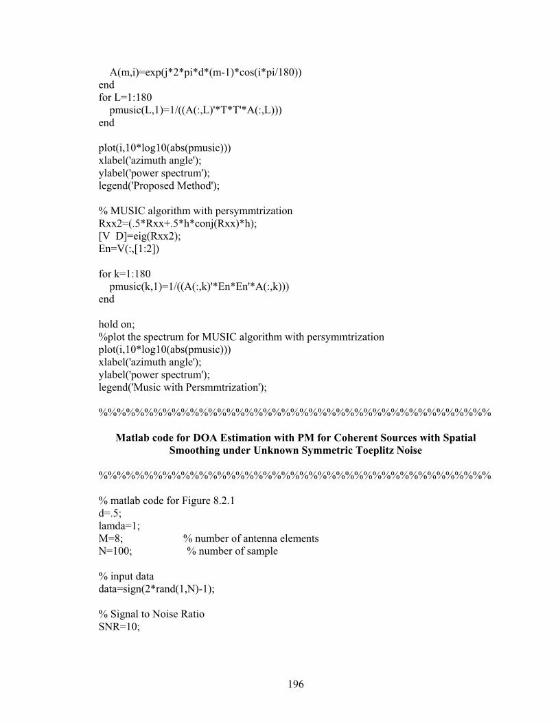
196
A(m,i)=exp(j*2*pi*d*(m-1)*cos(i*pi/180))
end
for L=1:180
pmusic(L,1)=1/((A(:,L)'*T*T'*A(:,L)))
end
plot(i,10*log10(abs(pmusic)))
xlabel('azimuth angle');
ylabel('power spectrum');
legend('Proposed Method');
% MUSIC algorithm with persymmtrization
Rxx2=(.5*Rxx+.5*h*conj(Rxx)*h);
[V D]=eig(Rxx2);
En=V(:,[1:2])
for k=1:180
pmusic(k,1)=1/((A(:,k)'*En*En'*A(:,k)))
end
hold on;
%plot the spectrum for MUSIC algorithm with persymmtrization
plot(i,10*log10(abs(pmusic)))
xlabel('azimuth angle');
ylabel('power spectrum');
legend('Music with Persmmtrization');
%%%%%%%%%%%%%%%%%%%%%%%%%%%%%%%%%%%%%%%%%%%
Matlab code for DOA Estimation with PM for Coherent Sources with Spatial
Smoothing under Unknown Symmetric Toeplitz Noise
%%%%%%%%%%%%%%%%%%%%%%%%%%%%%%%%%%%%%%%%%%%
% matlab code for Figure 8.2.1
d=.5;
lamda=1;
M=8; % number of antenna elements
N=100; % number of sample
% input data
data=sign(2*rand(1,N)-1);
% Signal to Noise Ratio
SNR=10;

197
% transmitted signal
s1=sqrt(10^(SNR/10))*data;
s2=(.4+.8i)*s1;
s3= (-.5-.7i)*s1;
s4=(.5+.6i)*s1;
s5=(-.3+.8i)*s1;
%DOA for incident sources
theta1=pi/180*40;
theta2=pi/180*50;
theta3=pi/180*60;
theta4=pi/180*70;
theta5=pi/180*80;
% generating covariance noise matrix in complex symmetric Toeplitz form
b=[1 -.9-.35*j .85-.32*j .75-.45*j .65+.48*j -.55-.35*j];
Q=toeplitz(b)
% generating exchange matrix h one’s in off diagonal elements and zero’s for all others
elements
w=eye(6);
h=[ w(:,6) w(:,5) w(:,4) w(:,3) w(:,2) w(:,1)];
% array response vector
i=[1:M];
A1=exp(-j*2*pi*d.*(i-1)*cos(theta1));
A2=exp(-j*2*pi*d.*(i-1)*cos(theta2));
A3=exp(-j*2*pi*d.*(i-1)*cos(theta3));
A4=exp(-j*2*pi*d.*(i-1)*cos(theta4));
A5=exp(-j*2*pi*d.*(i-1)*cos(theta5));
%the observation vector for subarray X
X=A1.'*s1+A2.'*s2+A3.'*s3+A4.'*s4+A5.'*s5;
X=Xr;
%phase delay for subarray Y
phiy1=exp(j*pi*cos(theta1));
phiy2=exp(j*pi*cos(theta2));
phiy3=exp(j*pi*cos(theta3));
phiy4=exp(j*pi*cos(theta4));
phiy5=exp(j*pi*cos(theta5));
%the observation vector for subarray Y
Y=A1.'*phiy1*s1+A2.'*phiy2*s2+A3.'*phiy3*s3+A4.'*phiy4*s4+A5.'*phiy5*s5;
Y=Yr;

198
%phase delay for subarray Z
phiy11=exp(2*j*pi*cos(theta1));
phiy22=exp(2*j*pi*cos(theta2));
phiy33=exp(2*j*pi*cos(theta3));
phiy44=exp(2*j*pi*cos(theta4));
phiy55=exp(2*j*pi*cos(theta5));
%the observation vector for subarray Z
Z=A1.'*phiy11*s1+A2.'*phiy22*s2+A.3'*phiy33*s3+A.4'*phiy44*s4+A.5'*phiy55*s5;
Z=Zr;
Rxx1=zeros(M,M);
for k=1:100
Rxx1=Rxx1+Xr(:,k)*Yr(:,k)';
end
Rxx1=Rxx1/100+Q;
Ryy1=zeros(M,M);
for k=1:300
Ryy1=Ryy1+Yr(:,k)*Xr(:,k)';
end
Ryy=Ryy1/100+Q;
Rzz1=zeros(M,M);
for k=1:300
Rzz1=Rzz1+z(:,k)*z(:,k)';
end
Rzz=Rzz1/300+Q;
% proposed covariance difference for coherent sources.
Rxx2=1/6*((Rxx+Ryy+Rzz)+h*conj(Rxx+Ryy+Rzz)*h)-h*Rxx.'*h;
% propagator Method
G=Rxx2(:,1:5);
H=Rxx2(:,6);
F=pinv(G)*H;
T=[F;-eye(1)];
% Spectrum to find DOA for proposed method
for m=1:M;
i=1:180;
A(m,i)=exp(j*2*pi*d*(m-1)*cos(i*pi/180))
end
for L=1:180
pmusic(L,1)=1/((A(:,L)'*T*T'*A(:,L)))

199
end;
% Figure 8.2.1
plot(i,10*log10(abs(pmusic)))
xlabel('azimuth angle');
ylabel('Power Spectrum');
legend('Proposed Method');
%forward-backward spatial smoothing method
Rxx2=((Rxx+Ryy+Rzz)+h*conj(Rxx+Ryy+Rzz)*h);
[V D]=eig(Rxx2);
En=V(:,[2])
for k=1:180
pmusic(k,1)=1/((A(:,k)'*En*En'*A(:,k)))
hold on;
% Figure 8.2.1
%plot the spectrum for forward-backward spatial smoothing method
plot(i,10*log10(abs(pmusic)))
xlabel('azimuth angle');
ylabel('Power Spectrum');
legend('Forward/backward Spatial Smoothing');
%%%%%%%%%%%%%%%%%%%%%%%%%%%%%%%%%%%%%%%%%%%
Matlab Code for Two-Dimension DOA Estimation with PM for Correlated Sources
under Unknown Symmetric Toeplitz Noise
%%%%%%%%%%%%%%%%%%%%%%%%%%%%%%%%%%%%%%%%%%%
% matlab code for Figure 8.3.2, 8.3.3, 8.3.4, and 8.3.5
%step 1 elevation angle estimation
d=.5;
lamda=1;
M=6; % number of antenna element
N=100; % number of snapshot
% input data
data1=sign(2*rand(1,N)-1);
data2=sign(2*rand(1,N)-1);
data3=sign(2*rand(1,N)-1);
data4=sign(2*rand(1,N)-1);
% Signal to Noise ratio
SNR1=10;
SNR2=10;
SNR3=10;

200
SNR4=10;
% transmitted signals
s1=sqrt(10^(SNR1/10))*data1;
s2=sqrt(10^( SNR2/10))*data1;
s3=sqrt(10^( SNR3/10))*data2;
s4=sqrt(10^( SNR4/10))*data2;
%DOA for incident sources
theta1=pi/180*60;
theta2=pi/180*75;
theta3=pi/180*80;
theta4=pi/180*85;
% generating exchange matrix h one’s in off diagonal elements and zero’s for all others
elements
w=eye(6);
h=[ w(:,6) w(:,5) w(:,4) w(:,3) w(:,2) w(:,1)];
% array response vector
i=[1:M];
A1=exp(-j*2*pi*d.*(i)*cos(theta1));
A2=exp(-j*2*pi*d.*(i)*cos(theta2));
A3=exp(-j*2*pi*d.*(i)*cos(theta3));
A4=exp(-j*2*pi*d.*(i)*cos(theta4));
% observation vector from the antenna elements in z-axis
Z=A1.'*s1+A2.'*s2+A3.'*s3+A4.'*s4;
Z=Zr;
Rzz1=zeros(M,M);
for k=1:100
Rzz1=Rzz1+Zr(:,k)*Zr(:,k)';
end
Rzz1=Rzz1/100
% generating of covariance noise matrix in symmetric Toeplitz form for the elements on
z-axis
b=[1 .9 .8 .7 .6 .5 ];
Q=toeplitz(b);
%The covariance matrix with noise
Rzz=Rzz1+Q;
% proposed covariance difference
Rzz2=(.5*Rzz+.5*h*conj(Rzz)*h)-h*Rzz.'*h;
% propagator Method

201
G=Rzz2(:,1:4);
H=Rzz2(:,5:6);
F=pinv(G)*H;
T=[F;-eye(2)];
% Spectrum to find DOA elevation angle for proposed method
for m=1:M;
i=1:180;
A(m,i)=exp(j*2*pi*d*(m-1)*cos(i*pi/180))
end
for L=1:180
pmusic(L,1)=1/((A(:,L)'*T*T'*A(:,L)))
end
% Figure 8.3.2
plot(i,10*log10(abs(pmusic)))
xlabel('Azimuth Angle');
ylabel('Power Spectrum');
% MUSIC algorithm
Rxx2=Rxx;
[V D]=eig(Rxx2);
En=V(:,[1:2])
for k=1:180
pmusic(k,1)=1/((A(:,k)'*En*En'*A(:,k)))
end
% Figure 8.3.4
%plot the spectrum for MUSIC algorithm
plot(i,10*log10(abs(pmusic)))
xlabel('Azimuth Angle');
ylabel('Power Spectrum');
%step 2 azimuth angle estimation
%DOA azimuth angle incident sources
phi1=(pi/180)*40
phi2=(pi/180)*50
phi3=(pi/180)*65
phi4=(pi/180)*70
% array response vector

202
i=[1:M];
B1=exp(-j*2*pi*d.*(i)*sin(theta1)*cos(phi1));
B2=exp(-j*2*pi*d.*(i)* sin(theta1)*cos(phi2));
B3=exp(-j*2*pi*d.*(i)* sin(theta1)*cos(phi3));
B4=exp(-j*2*pi*d.*(i)* sin(theta1)*cos(phi4));
% observation vector from the antenna elements in x-axis
X=B1.'*s1+ B 2.'*s2+ B 3.'*s3+ B 4.'*s4;
X=Xr;
Rxx1=zeros(M,M);
for k=1:100
Rxx1=Rxx1+Zr(:,k)*Zr(:,k)';
end
Rxx1=Rxx1/100
% generating of covariance noise matrix in symmetric Toeplitz form for the elements on
z-axis
d=[1 .95 .9 .85 .80 .75 ];
Q1=toeplitz(d);
%The covariance matrix with noise
Rxx=Rxx1+Q1;
% proposed covariance difference
Rxx2=(.5*Rxx+.5*h*conj(Rxx)*h)-h*Rxx.'*h;
% propagator Method
G1=Rxx2(:,1:4);
H1=Rxx2(:,5:6);
F1=pinv(G1)*H1;
T1=[F1;-eye(2)];
% Spectrum to find DOA azimuth angle for proposed method
elev =[ 60 75 80 85]
for s=1:length(elev)
for m=1:M;
i=1:180;
A(m,i,s)=exp(j*2*pi*d*(m-1)*sin(elev(s)*pi/180)*cos(i*pi/180))
end
for L=1:180
pmusic(L,1)=1/((A(:,L)'*T1*T1'*A(:,L)))
end
% Figure 8.2.3
plot(i,10*log10(abs(pmusic)))
xlabel('Elevation Angle');

203
ylabel('Power Spectrum');
% MUSIC algorithm for DOA azimuth angle
Rxx2=Rxx;
[V D]=eig(Rxx2);
En1=V(:,[1:2])
elevm =[ 45 67 86 93] % estimation of elevation angle for MUSIC algorithm.
for s1=1:length(elevm)
for m1=1:M;
i1=1:180;
A1(m,i,s)=exp(j*2*pi*d*(m1-1)*sin(elevm(s1)*pi/180)*cos(i1*pi/180))
end
for k1=1:180
pmusic(k1,1)=1/((A1(:,k1)'*En1*En1'*A1(:,k1)))
end
% Figure 8.2.5
%plot the spectrum for MUSIC algorithm
plot(i,10*log10(abs(pmusic)))
xlabel('Elevation Angle');
ylabel('Power Spectrum');