INVESTIGATION

Direct Testing for Allele-Specific ExpressionDifferences Between ConditionsLuis León-Novelo,* Alison R. Gerken,† Rita M. Graze,‡ Lauren M. McIntyre,§ and Fabio Marroni**,††,1

*Department of Biostatistics and Data Science, The University of Texas Health Science Center at Houston-School of PublicHealth, Texas 77030, †United States Department of Agriculture, Agricultural Research Service, Center for Grain andAnimal Health Research, Manhattan, Kansas 66502, ‡Department of Biological Sciences, Auburn University, Alabama36849, §Genetics Institute and Department of Molecular Genetics and Microbiology, University of Florida, Gainesville,Florida 32603, **Dipartimento di Scienze Agroalimentari, Ambientali e Animali, Università di Udine, 33100, Italy, and††Istituto di Genomica Applicata, 33100 Udine, Italy

ORCID IDs: 0000-0002-0077-3359 (L.M.M.); 0000-0002-1556-5907 (F.M.)

ABSTRACT Allelic imbalance (AI) indicates the presence of functional variation in cis regulatory regions.Detecting cis regulatory differences using AI is widespread, yet there is no formal statistical methodologythat tests whether AI differs between conditions. Here, we present a novel model and formally test differ-ences in AI across conditions using Bayesian credible intervals. The approach tests AI by environment (G·E)interactions, and can be used to test AI between environments, genotypes, sex, and any other condition.We incorporate bias into the modeling process. Bias is allowed to vary between conditions, making theformulation of the model general. As gene expression affects power for detection of AI, and, as expressionmay vary between conditions, the model explicitly takes coverage into account. The proposed model haslow type I and II error under several scenarios, and is robust to large differences in coverage betweenconditions. We reanalyze RNA-seq data from a Drosophila melanogaster population panel, with F1 geno-types, to compare levels of AI between mated and virgin female flies, and we show that AI · genotypeinteractions can also be tested. To demonstrate the use of the model to test genetic differences andinteractions, a formal test between two F1s was performed, showing the expected 20% difference in AI.The proposed model allows a formal test of G·E and G·G, and reaffirms a previous finding that cis reg-ulation is robust between environments.

KEYWORDS

robust regulationallelic imbalanceallele-specificexpression

gene regulatorynetworks

Regulatory variation can occurwithin cis acting regions (e.g., promoters,enhancers, and other noncoding sequences, directly altering expressionof a gene. Other trans acting factors such as transcription factors con-tribute to regulatory variation, but are expected to affect transcriptionof many target genes with which they interact. By revealing cis differ-ences in regulation and controlling for trans effects, allelic imbalance

(AI) provides a direct window into the relationship between cis regu-latory sequence and regulation of transcript levels (Brem et al. 2002;Yan et al. 2002; Lo et al. 2003; Wittkopp et al. 2004). Testing forregulatory variation that affects expression in cis is conceptuallystraightforward: two alleles within a heterozygote are compared toone another. If AI is observed, there is direct evidence of cis differencesbetween alleles; trans acting regulation alters expression of both allelesequally, producing an average effect across alleles at a locus, and doesnot contribute to AI within the heterozygote. Genetic interactions be-tween trans acting factors and cis regions are expected in some cases,and these interactions are not easily separated from cis effects.

Cis regulatory differences play a critical role in expression variationwithin populations (Rockman and Wray 2002; Stranger et al. 2012;Graze et al. 2014; Fear et al. 2016; Wang et al. 2017), divergence ofgene expression between species (Wittkopp et al. 2004; Graze et al.2009; McManus et al. 2010), parental imprinting (Crowley et al.2015), and in human health and disease (McCarroll et al. 2008; Linet al. 2012; Maurano et al. 2012). Importantly, many experimental

Copyright © 2018 Novelo et al.doi: https://doi.org/10.1534/g3.117.300139Manuscript received August 11, 2017; accepted for publication November 18,2017; published Early Online November 22, 2017.This is an open-access article distributed under the terms of the CreativeCommons Attribution 4.0 International License (http://creativecommons.org/licenses/by/4.0/), which permits unrestricted use, distribution, and reproductionin any medium, provided the original work is properly cited.Supplemental material is available online at www.g3journal.org/lookup/suppl/doi:10.1534/g3.117.300139/-/DC1.1Corresponding author: Dipartimento di Scienze Agroalimentari, Ambientali eAnimali, Università di Udine, Via delle Scienze 206, 33100 Udine, Italy. E-mail:marroni@appliedgenomics.org

Volume 8 | February 2018 | 447

designs have also incorporated comparisons across different physiolog-ical or environmental conditions (von Korff et al. 2009; Tung et al.2011; Cubillos et al. 2014; Buil et al. 2015; Chen et al. 2015; Fear et al.2016; Moyerbrailean et al. 2016; Knowles et al. 2017). Cis regulatorydifferences that are robust to environmental conditions, as well asapparent cis variant by environmental interactions, have been reportedin these and other studies. However, it is unclear if cis variation issimilar in most environments, or if there is a significant environmentalcomponent of variation in cis regulation. Current approaches rely oninformal comparisons of AI estimates made separately for each condi-tion, and there is no current formal test for AI by environmentinteraction.

One inherent, and often neglected, difficulty in measurement ofAI is to discriminate real allelic imbalance frombias in estimation ofAI, often due to differential mapping of the two alleles on thereference (Degner et al. 2009). Early studies of AI used simpledesigns consisting of two parental strains and a single F1 genotype,with expression measured under standard conditions. These stud-ies often used empirical controls (typically F1 DNA samples) toidentify bias in estimation of AI (Wittkopp et al. 2004; Graze et al.2009, 2012). However, sequencing DNA for many genotypes, inaddition to RNA samples for multiple genotypes and conditions,can be prohibitively expensive. Alternatively, parental DNA readscan be simulated for identification of some forms of bias (Degneret al. 2009; Stevenson et al. 2013; León-Novelo et al. 2014), and/ora range of bias can be examined for the impact on inferences (Fearet al. 2016). The use of a strain-specific reference or direct identi-fication of genetic variants from the data also improves the esti-mation of AI (Skelly et al. 2011; Turro et al. 2011; Graze et al. 2012;Satya et al. 2012; León-Novelo et al. 2014; Munger et al. 2014; Fearet al. 2016). These analytical approaches account for bias by fil-tering regions of likely bias, incorporating information from con-trols or simulations, or use both filtering and modeling (reviewedin Castel et al. 2015).

A variety of approaches have been taken to test for significant allelicimbalance in simple designs (Ronald et al. 2005; Degner et al. 2009;Zhang and Borevitz 2009; Gregg et al. 2010; McManus et al. 2010;Rozowsky et al. 2011; Skelly et al. 2011; Turro et al. 2011; Grazeet al. 2012; León-Novelo et al. 2014). Approaches have included linearmodels for array based studies (Ronald et al. 2005; Zhang and Borevitz2009), binomial or chi-square tests (Degner et al. 2009; Gregg et al.2010;McManus et al. 2010; Rozowsky et al. 2011), and Bayesianmodelsfor RNA-seq based studies (Skelly et al. 2011; Turro et al. 2011; Grazeet al. 2012; León-Novelo et al. 2014). The variance due to randomsampling reads from a library can be modeled by treating the totalnumber of reads in a biological replication as a random variable(Graze et al. 2012; León-Novelo et al. 2014).

For more complicated designs that include multiple genotypes,sexes, and/or environmental conditions, existing studies have pri-marily used two-stepmethods, applying an initial model to detect AIin each condition, and then a comparison to determine if AI differsbetween sample groups. This two-step method has been imple-mented for a variety of different approaches, including binomialtests with log odds ratios, likelihood ratio tests with Bayesian meta-analysis, and Bayesianmodels with pairwiseWilcoxon tests (Edsgärdet al. 2016; Fear et al. 2016; Moyerbrailean et al. 2016). For example,as part of their analyses, Fear et al. (2016) apply a Bayesian model todetermine AI, and identify the genes in AI across 49 test crosses offemale Drosophila melanogaster flies in only one environment, ei-ther virgin or mated. The approach proposed here is more general inthe sense that not only does it, as in Fear et al. (2016), determines AI

in mated and/or in virgin flies, but, in contrast to Fear et al. (2016), italso formally tests whether the levels of AI are significantly differentin the two environments.

We introduce here a novel Bayesian model (referred to as theenvironmental model) that allows formal testing of AI between envi-ronments, while accounting for potential bias, and model the totalnumber of reads as a randomsample from the library. Themodel can beused with or without empirical control samples to account for bias. Inaddition, the environmental model explicitly takes into account theexpression level of the genic region being examined in each condition, aswell as the proportion of reads that are informative for estimatingallele-specific expression. The ability to assign reads to the paternal ormaternal allele depends upon the amount and location of sequencedifferences observed between the alleles. The higher the number ofdifferences, and the more even the distribution, the greater thediscrimination ability. Lower numbers of differences or large regionswith nodifferences result in greater numbers of unassigned reads thatare not informative for estimation of AI. To our knowledge, in allanalyses of AI to date, reads uninformative for AI analyses arediscarded. The unassigned reads provide us information about thevariability of the read counts, and more precise estimate of thisvariance increases the power to detect AI.

To test theperformanceof themodelwith real data,wealsoconduct areanalysis of existing data, examining differences in AI for an environ-mental perturbation in Drosophila that has dramatic effects on overallexpression, the change from virgin to mated status. During mating,male D. melanogaster transfer, together with sperm, a mixture of pep-tides and proteins into the female reproductive tract; these peptidescause profound changes in female physiology (Zhou et al. 2014). Asa consequence, mated female flies experience changes in body compo-sition (Everaerts et al. 2010), life span (Aigaki and Ohba 1984), andgene expression (Lawniczak and Begun 2004; McGraw et al. 2008).Here, we use the environmental model to understand how this largephysiological change affects variation in cis regulation.

METHODS

The baseline modelThe baselinemodelwas developed by León-Novelo et al. (2014). Briefly,the observed read counts in biological replicate (i) for any singleexon/environment are assigned to maternal or paternal alleles, andunassigned reads are discarded (Figure 1). Let xi and yi be the RNAallele-specific read counts from a heterozygote in biological replicateiði ¼ 1; . . . IÞ :

yi��m;a;bi; q � PoissonðmabiqÞ; and

xijm;bi; q � Poissonðmbið12 qÞÞ:Here, m is the overall mean, bi is the variation of biological replicates(i ¼ 1; . . . ; I) due to the random sampling of reads from libraries,a is the effect of a read having AI, and q incorporates bias informa-tion, where values .0.5 indicates bias toward the y allele, andvalues ,0.5 is bias toward the x allele. If u is the real proportion ofreads from the y allele then:

u ¼ mabi

mbi þ mabi¼ a

1þ a;

when there is no AI (u ¼ 0:5), therefore a ¼ 1: The bias correctionparameter is q; it can be a random variable estimated from DNAcontrols, from simulation, or a fixed constant varied to reflect un-certainty (Fear et al. 2016).

448 | L. León-Novelo et al.

The environmental modelLet i = 1,2 be the index of condition, which can represent environ-mental differences or differences in treatments (e.g., mated andvirgin status) or differences between genotypes. We define themas environment 1 and environment 2.

Assume that we haveK1 biological replicates for environment 1 andK2 replicates for environment 2.

For each gene/gene region to be examined, we define:

xi,k = number of RNA reads aligned to the “maternal” allele inenvironment i and replicate k,

yi,k = number of RNA reads aligned to the paternal allele.zi,k = number of RNA reads aligned equally well to both alleles, and

that cannot be assigned to either allele; they are also referred to as“unassigned”; and

ri,p (ri,m) = probability that a read generated from paternal (mater-nal) aligns to paternal.

(maternal) for environment i. In specific notation:ri,p = Pr[read aligns to paternal|read generated by paternal] for

i = 1,2.12ri,p = Pr[read is unassigned|read generated by paternal] for the

genotype in environment i.

ri,p (ri,m) can be estimated from control DNA or from simulation.To estimate ri,p, (1) use the paternal genome to simulate all possiblereads that can be generated by the paternal allele, (2) align these reads to

both the paternal and maternal genomes, and (3) estimate ri,p as theproportion of the simulated reads aligning best to the paternal genome.Note that the true proportion of simulated reads aligning best to theparental allele in the two environments (r1,p and r2,p) for the samegenotype is expected to be similar. However, to allow for comparisonsacross genotypes where this assumption may not hold, the model doesnot force these two parameters to be identical.

We assume that the distribution of the counts xi,k; yi,k; zi,k|ai, bi,khave the expected values given in Table 1. A graphical representation ofthe expected values is provided in Figure 1. The biological replicationspecific random effect bi,k corrects for the random sampling of readsfrom the library for each biological replication. As with the baselinemodel, we assume that the total number of reads from a biologicalreplication is a random effect with expected value bi;kðai þ 1=aiÞ: Thisexplicitly recognizes the sampling of material from a library in order togenerate the observed reads and incorporates the resulting samplingvariance directly into the model. Approaches that consider the totalnumber of reads in a biological replication to befixed often fail tomodelthe overdispersion of the data. Allowing it to be random allows mod-eling of the overdispersion.

For example, the maternal read count of the third virgin replicate,x2;3; has an expectation of a2b2;3r2;m: Note that when ri,p and ri,m areboth equal to 1, we expect all the reads to be assigned to an allele, andthe proportion unassigned to be zero (i.e., zi,k = 0). The proportion ofreads assigned to the maternal (paternal) allele compared to those that

Figure 1 Read assignment. Reads aligning tothe maternal allele (m) are purple, those align-ing to the paternal allele (p) are green, andthose aligning equally well to both alleles (un-assigned) are gray. Expected values accord-ing to the environmental model are given inTable 1, and are in black type above. Thebaseline model uses information of the readsaligning to paternal or maternal alleles only(red boxes), while the environmental modeladditionally incorporates information aboutunassigned reads (blue boxes). In thebaseline model, m is the overall expectedvalue, bk models the biological replicatevariation, a 6¼ 1 is equivalent to AI, and theknown quantity 12q is interpreted as theexpected proportion of maternal read countswhen there is no AI. In other terms,Eðx=ðy þ xÞja ¼ 1Þ ¼ 12q: The priors for allmodel parameters are gamma(1/2,1/2).The quantities

ffiffiffia

pmbk and 1=

ffiffiffia

pin the

notation of the baseline model play therole of the parameters bk=ðrm þ rpÞ and a

respectively in the environmental model.When a ¼ 1 in the environmental model,E ðx ja ¼ 1Þ=E ðx þ y ja ¼ 1Þ ¼ rm = ðrm þ rpÞ:This leads us to an interpretation of q underthe null in the baseline model as rp=ðrm þ rpÞin the environmental model.

Volume 8 February 2018 | Allelic Imbalance Between Conditions | 449

are not assigned will depend on several factors, such as read length, thelevel of divergence between the two haplotypes, the alignment algo-rithm, and the stringency of alignment. These parameters are not equalto reflect the possibility that the quality of the genotype specific refer-ences may not be equivalent between the maternal and paternal refer-ence, and/or that for a particular gene/gene region there may beunobserved structural variation in one but not both alleles. DNA con-trols can account for factors such as hidden structural variation, but canbe prohibitively expensive. In the absence of DNA controls, the use ofsimulations can estimate some of the potential bias, and inclusion ofthese estimates in the model is preferable to ignoring sequence andmapping bias altogether (León-Novelo et al. 2014).

bi,k/ai and aibi,k are the total expected number of reads from thepaternal and maternal alleles, respectively, in environment i and bi-ological replication k. Of the bi,k/ai reads coming from the paternalallele, we expect (1/ai)bi,kri,p to be assigned to the paternal allele, and(12ri,p)bi,k/ai to be unassigned. Similarly, of the aibi,k reads fromthe maternal allele, we expect aibi,kri,m to be assigned to the mater-nal allele and (12ri,m)aibi,k to be unassigned. The parameter a2

i isthe ratio of the maternal and paternal expected value counts forgenotype i, after adjusting for assignment bias. Explicitly allowingfor reads to be unassigned allows the level of expression to be in-cluded in the modeling.

The notation is the following:

a2i ¼

E�xi;k

��ri;m

E�yi;k

�.ri;p

;

for i = 1,2 and k = 1,2,. . .,Ki.We are interested in testing the null hypotheses:

1. Allelic balance in environment 1 (e.g., mated) or, equivalently, H01:a1 = 1.

2. Allelic balance in environment 2 (e.g., virgin), H02: a2 = 1.3. The level of AI is the same in both (or independent of) environ-

ments. Equivalently, H03: a1 = a2.

Notice that H03 is testing if the true proportion of reads comingfrom the paternal allele in environment 1 (e.g., mated) is the same as inenvironment 2 (e.g., virgin), or, in other words, the level of AI is thesame in both conditions (e.g., mated and virgin). This is a formal test forthe interaction between AI and environment.

The proportion of counts coming from the maternal allele (line) inenvironment i is then:

ui ¼E�xi;k

�ri;m

�E�xi;k

�ri;m þ yi;k

.ri;p

� ¼ ai

ai þ 1=ai:

ui is expected to be 0 when no counts are coming from the maternalallele, 1 when all the counts are coming from the maternal allele, and0.5 in the case of perfect allelic balance. The model is implemented inR (R Core Team 2017), and is available as Supplemental Material,File S2.

Negative binomial sampling modelAbove, we describe themodel for the expected value counts, and nowwemodel the counts. We assume the counts follow a negative binomialdistribution, with expected values given in Table 1. For example, thedistribution for the read counts in the third virgin biological replicatealigning to the maternal allele is:

x2;3 � NB�mean ¼ r2mb2;3a2; dispersion ¼ f

�:

The dispersion parameter f is common to the distribution of all readcounts. Here x � NBðm;fÞ denotes the negative binomial distribu-tion with mean m and variance mþ fm2: RNA-Seq data typicallyexhibit overdispersion (with respect to the Poisson model; i.e., thevariance is greater than the mean). Since the negative binomialsampling distribution can model overdispersed data, it has beenproposed as a sampling distribution for RNA counts (Robinsonand Smyth 2007; Anders and Huber 2010; Di et al. 2011; León-Novelo et al. 2017).

To complete the Bayesian model, we specify the prior distributionsfor the model parameters:

a1;a2 � lognormal�ma ¼ 0;s2

a ¼ 1�42�

b1;1 ; . . . ;b1;K1;b2;1; . . . ;b2;K2

� gamma�ab ¼ ~ab; bb

�

bb � gamma

abb ¼ 2; bbb ¼ 2 ~bb

f � Inverse2 gamma�af ¼ 2:01; bf ¼ 0:05

�:

Here, gammaða; bÞdenotes the gamma distribution with mean shapeand rate parameters a and b:

The computation of credible intervals for the parameters of interesta1;a2 and a1=a2 is carried out using Markov Chain Monte Carlo. WerejectH01when the credible interval fora1does not contain 1. Similarly,we reject H02 (or H03) when the credible interval fora2 (ora1=a2Þ doesnot contain 1.

The lognormal prior distributions for the parametersa1anda2 wereused to make the model symmetric with respect to the labels paternaland maternal (in our example, tester and line, respectively). This is apriori ai � 1=ai so the estimates of ai in the baseline model are thesame as the estimates of 1=ai in the model swapping the labels of testerand line. The hyper-parameter s2

a ¼ 1=42 is chosen so that the priorexpected value of ai equals ma þ expðs2

a=2Þ ¼ 1:03 � 1; and priorvariance ðexpðs2

aÞ2 1Þ · expð2ma þ s2aÞ ¼ 0:4168; so, in the case of

noninformative data (e.g., very small counts), the posterior distributionof ai is similar to the prior, and we do not conclude AI. The gammaprior for bb “tightens” the biks to be similar.

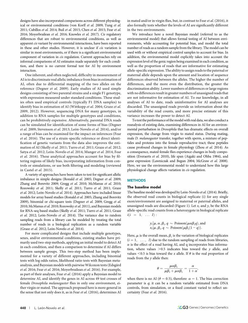
n Table 1 Expected values for read counts under the proposedmodel for environment i and replicate (i, k), where i = 1, 2 and k =1,2. . ..ki

Maternal (xi,k) Paternal (yi,k) Unassigned (zi,k)

aibi,kri,m (1/ai)bi,kri,p [(12ri,p)/ai + (12ri,m) ai]bi,k

Every replicate produces three observed counts for each gene/gene region: onefor reads aligning better to the maternal allele, one for reads aligning better tothe paternal allele, and one for reads aligning equally well to both alleles, andtherefore unassigned to either the paternal or maternal allele. The sum of theexpected counts will be the expected total number of reads aligned to thatgene/gene region and an estimate of overall expression. Note that the numberof reads is considered random to account for variation due to sampling readsfrom the library.

n Table 2 Values of b used in the simulations

k = 1 k = 2 k = 3

i = 1 1 1.2 0.7i = 2 1 1.3 0.8

450 | L. León-Novelo et al.

Setting a prior in the hyper-parameters of the prior distribution ofbiks allows a “borrow of strength” across different biological replicates.To set the hyper-parameters of the prior distribution for bb; we usean “empirical Bayes approach.” First, we obtain (rough) estimatesfor biks. Second, we assume that they follow a gamma distribution,and compute the MLE estimates ab and bb of the shape and rateparameters, respectively. Third, we set the parameter in the modelab[ab; and we set abb ¼ 2bb and bbb ¼ 2 so that EðbbÞ ¼ bb andvarðbbÞ ¼ 2bb: Since we have few data points to estimate f; we usean informative prior with mean bfðaf 2 1Þ � 0:05 prior with var-iance b2f=½ðaf21Þ2ðaf 2 2Þ� � 0:05:

Measuring type I and II error rateRead counts were simulated according to a negative binomial distribu-tion in several different scenarios. In each scenario, read counts weresimulated for 1000 gene regions (for convenience, we refer to these asexons) independently in two different environments, with three repli-cates per environment. The number of readsmapping in each exon wassimulated according to a negative binomial distribution with size = 50and expected value equal to bi,k · h, where bi,k is the effect of bi-ological replicate in environment i and replicate k, and h is a factorused to simulate different levels of gene expression (and/or sequencing

coverage), which in turn affect the power of detecting AI. Simulationswere run with h = 10 (low expression/coverage) and h = 100 (highexpression/coverage). bi,k was varied as shown in Table 2.

Different levels ofAI in the environment 2were simulated for sets of1000 exons by varying a2 from 0.5 to 2. No AI was simulated inenvironment 1 (i.e., a1 = 1); 11 different levels of log2 of the ratio a1

/a2 were simulated, varying from 21 and 1 with step 0.2.Read counts were simulated without bias, i.e., with rp = rm. To

assess robustness of the model to misspecification of bias, unbiasedsimulated counts were fed to the model, and analysis of AI was con-ducted after providing biased prior estimates of rp and rm.

The bias in estimation of AI is not always correctly captured bysimulation or byDNAcontrols. Thismeans that, evenwhen controls areused, bias may be mis-specified. It is important to understand how themodel performs with different levels of mis-specification. Bias mis-specification was measured as x = 2(100)(r21), where (r21) is thedifference between the mis-specified value of rp (or rm) used to fit themodel, and the simulated value of rp (or rm), i.e., 1. Nine different levelsof mis-specification x were used: 240, 230, 220, 210, 0, 10, 20, 30,and 40%.

When maternal and paternal alleles have similar sequences in thecoding region, the proportion of reads aligning equally well to both

Figure 2 Type I error rate. The two upper panels show Type I error rate in the case of low gene expression, and the two bottom panels showType I error rate in the case of high gene expression. Panels on the left show results obtained by specifying the number of reads aligning equallywell to both alleles as expected under the model in Table 1. Panels on the right shows results obtained by multiplying that quantity by 10,000. Weplot in red the type I error rate in environment 1, in gray the type I error rate in environment 2, and in blue and green the type I error rate indetecting different levels of AI between environments using the Bayesian approach implemented in the environmental model, and the descriptivemethod as implemented in the baseline model, respectively. Low expression: h = 10; High Expression: h = 100; Low unassignment: unassignedreads = zi,k; High unassignment: unassigned reads = 10,000 · zi,k

Volume 8 February 2018 | Allelic Imbalance Between Conditions | 451

alleles is high. A series of simulations was conducted using theexpected number of unassigned reads zi,k. To assess the effect ofvariation in the proportion of unassigned reads, an additional seriesof simulations was conducted by multiplying the expected values ofzi,k by 10,000. We will refer to these two scenarios as “unassignedinflation factor = 1” and “unassigned inflation factor = 10,000,”respectively.

The first scenario can be observed when the paternal and maternalhaplotypes are different, and most reads can be assigned. The secondscenario is observedwhenmost of the reads cannot be assigned to eitherhaplotype, and is used as a worst case scenario of very similar paternaland maternal haplotypes. In any given experiment, we expect somegenes to follow each of these two scenarios.

Tomeasure the robustness of the model to unequal gene expressionacross conditions,we repeated the simulations comparingoneconditionwith high coverage, and one with low coverage, i.e., we run a simulationsettingh1 = 10 andh2 = 100, and a simulation settingh1 = 100 andh2 = 10. This is an important consideration as differential expressionshould not be confused with AI.

Type I error was assessed using simulations in which a1 = 1 anda2 = 1 (i.e., no AI in either environment). Type II error of AI detection,

and of the detection of difference in AI across environments, wasassessed using simulations in which a1 = 1 and a2 6¼ 1.

Reanalysis of D. melanogaster data (mated vs. virgin)

Data retrieval and cleaning: RNA-seq data from a panel of 68 D.melanogaster F1 hybrids obtained from crossing 68 strains with thew1118 laboratory strain (Kurmangaliyev et al. 2015) were used to mea-sure allele specific expression. Mapping of reads on genotype-specificreferences and quantification of reads aligning to each exon was per-formed as previously described (Fear et al. 2016). Briefly, reads origi-nating from each cross were aligned on the strain-specific references

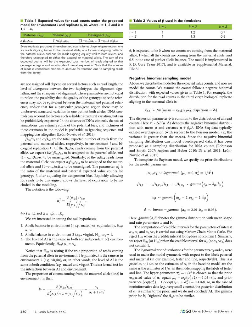
Figure 3 Type II error rate. Type II error rate when comparing an environment for which no AI was present (a1 = 1) with an environment withvarying levels of AI. Differences in AI between environments are reported as log2 a1/a2. The two upper panels show Type II error rate in caseof low gene expression, and the two bottom panels show Type II error rate in case of high gene expression. Panels on the left show resultsobtained by specifying the number of reads aligning equally well to both alleles as expected under the model in Table 1. Panels on the rightshows results obtained by multiplying that quantity by 10,000. We plot in red the type II error rate in environment 1, in blue the type II errorrate for difference in AI between environments, and in green the type II error rate between the environments when using the descriptiveapproach as implemented in the baseline model. Each point represents the average over the seven simulated levels of bias misspecification,and the error bars represent SE. Low expression: h = 10; High Expression: h = 100; Low unassignment: unassigned reads = zi,k; Highunassignment: unassigned reads = 10,000 · zi,k

n Table 3 Number of data points (exons 3 lines) showing AI

Mated Environmental a = 1 Environmental a 6¼ 1

Baseline a = 1 46,544 3574Baseline a 6¼ 1 5853 6477Virgin Environmental a = 1 Environmental a 6¼ 1Baseline a = 1 46,353 3514Baseline a 6¼ 1 5962 6619

452 | L. León-Novelo et al.

(obtained from FlyBase v5.51) for the two parental genomes, and readswere classified as aligning in paternal (tester), maternal (ine), or un-assigned (when reads mapped equally well on both references).

Based on simulations, low numbers of reads assigned tomaternal orpaternal allele, and/or high numbers of reads that cannot be assigned toeither allele lead to inflated type I error. For this reason, instances inwhich the proportion of total reads assigned to either parental allelewas,1% (i.e., having either very low number of assigned reads or veryhigh number of unassigned reads) were excluded from analysis.

Analysis was performed on a total of 169,842 data points (termed“exons · lines,” i.e., the number of exons across all lines), belonging to13,898 different exons in 68 crosses. In the manuscript, the terms “datapoint” and “exons · lines” will be used to indicate the sum of infor-mative lines across all the informative exons (or equivalently, the sumof informative exons across all the informative lines), as follows:

Data  pointsðexons · linesÞ ¼Xni¼1

Xmj¼1

eilj;

where ei and lj are 1 if exon i in line j is informative and zero otherwise,and n and m are the total number of exons and lines considered,respectively.

For thepurposeof analysis, datawere aggregatedby (a) exon, (b) line,or (c) exon in line. We detail below the different meanings. One genecomposed of two exons, onewith data in 10 crosses, andonewith data in15 crosses, respectively, has information in two exons, in 12.5 lines(average) and 25 data points. A gene consisting of 25 exons, all with datain just one cross, is said to have information in 25 exons, one line, and25 data points.

Comparing the environmental model with the baseline model:A Bayesian model that accounts for bias (León-Novelo et al. 2014) hasbeen already applied to the D. melanogaster data presented here (Fearet al. 2016); we will refer to it as the “baseline” model. The modelpresented here extends the baseline model significantly, and directly

compares AI between environments; it will be referred to as the “envi-ronmental” (as opposed to the “baseline”) model. Results were com-pared for a total of 66,504 data points that passed quality control inboth the previous (Fear et al. 2016) and present study. Pearson’s cor-relation coefficients between the posterior estimates of the proportionof reads aligning on the paternal allele (q) were estimated for mated

Figure 4 Posterior estimate of q. Posterior estimate of q according to the baseline and environmental model in mated (left) and virgin (right) flies,respectively. Each dot represents a data point. Black points: no AI in either set. Red Points: AI detected by baseline model alone. Blue points: AIdetected by environmental model alone. Purple points: AI detected by both models. Blue line: bisector of the first quadrant angle. Red line:regression line.

Figure 5 Exon coverage and AI. Base 10 logarithm of coverage ofexons for which no model detected AI (gray boxes), only the environ-mental model detected AI (yellow boxes), only the baseline modeldetected AI (dark red boxes), or both models detected AI (orangeboxes), respectively.

Volume 8 February 2018 | Allelic Imbalance Between Conditions | 453

and virgin flies according to results of the baseline and environmentalmodel, respectively.

To determine the effect of coverage (number of reads mapped oneach exon) on AI in the baseline and environmental model, exons werestratified into four groups: (1) no AI according to either model, (2) AIaccording to the environmental model only, (3) AI according to thebaseline model only, and (4) AI in both models. Mean coverage was

assessed by measuring the mean number of reads mapping an allelespecifically in each exon in mated and virgin lines. The distribution ofcoverage among exons without AI was compared to the distribution ofcoverage in the remaining three classes using the Wilcoxon-Mann-Whitney test, separately for mated and virgin flies. The distribution ofthe deviation of q from the expected value of 0.5 was plotted in exonsshowing, or not showing, AI in either model in virgin and mated flies,

Figure 6 Deviation from expected q and AI. Distribution of the absolute value for the deviation of q from the expected value of 0.5 in exons forwhich AI was detected (a = 1) or not (a 6¼ 1), according to the baseline (light pink) or environmental model (dark red). Differences betweengroups according to Wilcoxon pairwise test are shown. Groups sharing a letter are not different. Groups not sharing letters are different.

Figure 7 BA plot. BA plot comparing esti-mates of q according to the baseline (Base)and environmental (Env) model in mated andvirgin flies, respectively. The red line repre-sents the mean difference. The dotted linesare the 95% confidence intervals of the differ-ence. The regression of the difference overthe mean is represented by the blue line.

454 | L. León-Novelo et al.

separately. The distribution of the differences in the estimate of q be-tween the two models were plotted, stratifying AI classification accord-ing to the two models: no AI, AI according to either one of the models,AI according to both models. Statistical analysis were performed in R(R Core Team 2017).

Analysis of AI in mated and virgin flies using the environmentalmodel: The RNA-seq data included in this study has been describedbefore (Kurmangaliyev et al. 2015). Briefly, RNAwas obtained from F1mated and virgin flies originated by crossing females of each of 68 lineswith mates of a common tester (w1118). Data points were included in

the study if at least 50 reads could be mapped to either paternal ormaternal allele in both virgin and mated flies, and if at least 200 totalreads weremapped to the exon (irrespectively of thembeing assigned tothe paternal or maternal allele, or being unassigned). The environmen-tal model was used to simultaneously estimate AI in mated female flies,in virgin female flies, and to test for AI by environment interaction(G·E). In total, 169,842 data points were analyzed.

As each of the F1 genotypes has been evaluated for AI, it is of interestto assess the population frequency of AI in any given exon, Fisher’sexact test was performed on a 2 · 2 contingency table, reporting foreach exon and the number of F1 genotypes showing different levels of

Figure 8 Model comparison. Distribution of absolute difference in q estimates between mated and virgin flies in several contrasts according todifferent models. Both a = 1: AI not detected in mated nor virgin flies. One a = 1: AI detected in onemating status alone. Both a 6¼ 1: AI detectedin both mated and virgin flies. Classifications are based on results obtained by the baseline model, for which the difference in AI betweenenvironments is reported using a descriptive approach (red), the environmental model, using the descriptive approach for describing differencein AI (dark blue), and the environmental model, using a formal Bayesian test of the null hypothesis for detecting difference in AI (light blue).

Volume 8 February 2018 | Allelic Imbalance Between Conditions | 455

AI between conditions and those not showing differences inAI betweenconditions. Exons showing higher (or lower) than expected frequencyof AI between conditions were identified by testing the hypothesis thatthe odds ratio in the contingency table is .1 or ,1.

A further demonstrative analysis of how genotypes may be comparedacross the population was performed by explicitly comparing AI in twodifferent F1 genotypes, treating each F1 genotype as an environment. TheenvironmentalmodelwasusedtosimultaneouslyestimateAIinr365·w1118F1’s, in r907·w1118 F1’s, and to test for AI by F1 interaction (G·G).

Data availabilitySequences used for the presentworkwere retrieved from SRAunder theaccession number PRJNA281652. Detailed description of the proce-dures for obtaining F1 genotypes is available at https://github.com/McIntyre-Lab/papers/tree/master/lehmann_2015/original_data. File S1

includes supplemental methods, Figures S1–S5 in File S1 with leg-ends, and Table S1 in File S1 with legend. The supplemental materialincludes an implementation of the model in R and a toy data set.Instructions are provided in File S2.

RESULTS AND DISCUSSION

Measuring type I and II error rate of theenvironmental modelWe assessed type I and II error simulating various scenarios thatcould be experienced in real experiments. We varied h, a proxy ofthe number of reads mapped to each feature, and thus represen-tative of the combination of gene expression and average sequenc-ing depth (coverage). In addition, we varied the proportion ofreads that cannot be assigned to either allele (unassignment). High

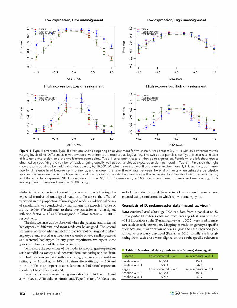
Figure 9 Comparison of AI detected in mated and virgin flies by the two models. Numbers represents the number of genes. A gene wasclassified as having a 6¼ 1 when at least one exon in at least one line had a 6¼ 1.

456 | L. León-Novelo et al.

unassignment rates can be observed when the paternal and ma-ternal allele are similar, and a large proportion of reads cannot beunambiguously attributed to either allele.

Results shown in Figure 2 report Type 1 error rate as a function ofbias misspecification at two different levels of gene expression (or cov-erage), and two different levels of unassigned reads. Unlike the baselinemodel, the type I error rate when the number of unassigned readsfollows the model expectation (Table 1), and the bias is not higher thanpreviously reported in interspecific crosses, where it has beenmeasuredby DNA (Graze et al. 2012; León-Novelo et al. 2014), is close to theexpected nominal levels.

Only when the number of unassigned reads is 10,000 times theexpected value (Table 1), do type I error rates climb. As expected, whenbias is high, and unaccounted for in themodel, the type I error rate canbe very high. Under this “worst case” scenario, the environmentalmodel still has lower type I error relative to the baseline model.

When the number of unassigned reads matches the model expec-tation (Table 1), the type I error rate for detecting differences in AIacross environments (blue lines and dots in Figure 2) is,5% for all biasmisspecification levels.

As expected, the type II error rate increases when log2 a1/a2 ap-proaches zero. At each value of log2 a1/a2, lower expression leads to ahigher type II error rate. The effect of the misspecification of the pro-portion of unassigned reads on type II error is small (Figure 3).

Further analyses were performed simulating 10-fold differencein coverage between conditions. When higher coverage occurs inenvironment 2 (Figure S1 in File S1 left panel), type I error in envi-ronment 2 is higher, and vice versa (Figure S1 in File S1 right panel).The detection of differences in AI between environments might benegatively affected by different levels of coverage across the experi-ments. Our simulations show that in this case, as previously reported,the baseline model has a high type I error while the environmentalmodel has very low type I error (Figure S1 in File S1). This suggeststhat the environmental model does, as expected, protect from type Ierror under different coverage levels. Correspondingly, the Type IIerror is higher for the environmental model compared to the baselinemodel. This is especially true when the difference in a is small (FigureS2 in File S1).

Reanalysis of D. melanogaster data

Comparing the environmental model with the baseline model: Weprovide here a comparison of the results from the environmental modelto those published using the baseline model (Fear et al. 2016), foranalysis of differences inAI acrossmated and virgin physiological statesand F1 genotypes. A total of 62,448 data points (4880 different exonsand 49 different lines) were included in the final analysis. On average,each exon had detectable expression in 14 lines (ranging from 1 to

49 detected), and each line contains 1375 exons (ranging from 446 to2832 detected). Figures S3 and S4 in File S1 show, for each of the49 lines, the proportion of exons flagged with AI in mated and virginflies, respectively. The figures suggest that the two models have similarbehavior in the analyzed lines, with the environmental model beinggenerally more conservative and showing less extreme differencesacross lines. According to the environmental model, line r907 has thehighest proportion of exons with AI both in mated (44%) and virginflies (44%). According to the baseline model, line r907 has the highestproportion of exons with AI in mated flies (42%), and line r502 has thehighest proportion of exons with AI in virgin flies (46%).

Table 3 reports the number of data points showing AI in mated andvirgin flies, according to the baseline and environmental models, re-spectively. In general, the baseline model is less conservative than theenvironmental model, detecting 12,330 and 12,581 events of AI inmated and virgin flies, respectively, vs. 10,051 and 10,133 detected bythe environmental model. Cohen’s kappa (Cohen 1960) between thetwo models is 0.49 in bothmated and virgin flies. Posterior estimates ofq were strongly correlated between the two models, with R2 of 0.92 inboth mated and virgin flies (Figure 4).

We compared coverage of exons stratified by significance according toeither environmental or baseline model. According to Wilcoxon’s test,coverage in exons not showing AI in either model was significantly lowerthan all other classes (Figure 5). The result is expected, since genes withlow coverage are expected to provide lower power for the detection of AI(León-Novelo et al. 2014). Exons showing AI only according to thebaseline model had higher coverage than all the remaining categories.This might be due to false positives in the baseline model. Simulationresults showed that the power of the environmental model increases ascoverage increases, with a relatively constant type I error rate, while thebaseline model has an increase in type I error at higher coverage. This islikely due to the inclusion of the unassigned reads as an estimate ofcoverage in the environmental model. The coverage of exons for whichonly the environmental model showed AI and of exons for which bothmodels detected AI, did not differ significantly.

As expected, the estimated deviation in AI from the null expectationis greater in exons for which AI was detected in bothmodels (Figure 6).

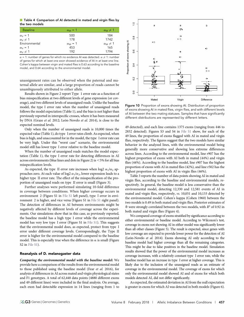
Figure 10 Proportion of exons showing AI. Distribution of proportionof exons showing AI in mated flies, virgin flies, and with different levelsof AI between the two mating statuses. Samples that have significantlydifferent distributions are represented by different letters.

n Table 4 Comparison of AI detected in mated and virgin flies bythe two models

Baseline aM = 1 aM 6¼ 1

aV = 1 500 184aV 6¼ 1 178 1742Environmental aM = 1 aM 6¼ 1aV = 1 453 165aV 6¼ 1 192 1794

a = 1: number of genes for which no evidence AI was detected. a 6¼ 1: numberof genes for which at least one exon showed evidence of AI in at least one line.Cohen’s kappa between virgin and mated flies is 0.63 according to the baselinemodel, and 0.64 according to the environmental model.

Volume 8 February 2018 | Allelic Imbalance Between Conditions | 457

In addition, exons in which AI was detected by the environmentalmodel showed higher median deviation than exons for which AI wasdetected by the baseline model. No significant difference between base-line and environmental model was observed for the estimates of q inexons without AI.

Figure 7 shows the BA plot comparing the two methods (Altmanand Bland 1983). The plot shows that a minority of data points elicitdifferent estimates ofq between baseline and the environmental model,especially for intermediate estimates ofq. We compared the number ofdata points for which differential AI between conditions was detectedby the environmental and baseline models stratifying by discrepancy inq estimates (Table S1 in File S1). Data points with a difference in qestimate (i.e., those lying outside of the 95% confidence interval)showed stronger disagreement between the environmental and thebaseline model in detecting differential AI across conditions (Fisher’sexact test p-value = 7.01E207 for data stratified by difference in qestimates inmated flies, and p-value = 2.27E206 for data stratified bydifferences in virgin flies). The difference is mainly due to instances inwhich the baseline model detects differences in AI and the environ-mental model does not (p-value = 2.62E207 and p-value = 1.79E205for estimates of q in mated and virgin flies, respectively). Instances inwhich the environmental model alone detects differential AI betweenconditions do not vary between points lying inside or outside of theconfidence intervals (p-value = 0.87 and p-value = 0.07 for estimatesof q in mated and virgin flies, respectively). This means that when theestimates of q differ, the baseline model shows a smaller difference in AIacross conditions.

The baseline model uses a descriptive approach to consider AIdifferences in mating status, by which an exon is classified as showing

different AI values in the two statuses, if and only if, it shows AI only inone status. This descriptive approach can be applied to the environ-mentalmodel (in addition to the explicit test of the null hypothesis), andwe implemented this approach to further compare the two models.

Using the baseline model, different AI between environments isdeclaredwhenAI is present in one of the two environments alone; usingthe environmental model, it is possible to both identify significantlydifferent levels of AI between environments with a direct test, andindirectly as a comparison between the individual tests within eachenvironment. Using the three possible approaches, we plot in Figure 8the distribution of q in exons for which no AI was detected (Botha = 1), AI was detected in one environment (One a = 1), and AIwas detected in both environments (Both a 6¼ 1).

The expectation is that, when the models detected AI in oneenvironment and not in the other (coded here as “One a = 1”), thedifference in theq distributions is greater than for other situations. Thiswas the case for all the approaches, but the larger difference was ob-served with the direct test of the null hypothesis a1 = a2 in the envi-ronmental model (Coffman et al. 2003).

We counted the number of genes for which at least one exon showedAI in at least one line in mated and virgin flies, respectively; results areshown in Figure 9 and Table 4.

Analysis of AI in mated and virgin flies using the environmentalmodel: Analysis of AI using the environmentalmodel was performedon a total of 169,842 exons in lines, belonging to 13,898 differentexons in 68 crosses. On average, each exonwas analyzed in 12 crosses

n Table 6 List of the 20 exons showing the least proportion ofdifferences in AI between mating statuses

Genea ChrbExonStartc

ExonEndd Counte

AIDifff P Diffg

Rack1 2L 7,826,534 7,826,981 68 0 0.007CG13868 2R 16,196,282 16,197,251 66 0 0.009eIF-4a 2L 5,985,026 5,985,793 63 0 0.011HmgZ 2R 17,584,993 17,585,809 63 0 0.011RpS24 2R 18,528,031 18,528,610 61 0 0.012Neb-cGP|nocte

X 10,355,115 10,359,100 58 0 0.015

CG5210 2R 12,579,123 12,579,404 57 0 0.016Gpdh 2L 5,947,240 5,948,843 57 0 0.016GstE9|imd 2R 14,296,553 14,297,838 57 0 0.016CG3198 X 6,562,736 6,566,212 56 0 0.018CG4577 2L 1,139,829 1,141,156 55 0 0.019CG7378 X 18,802,917 18,805,876 55 0 0.019CG9140 2L 6,062,079 6,062,435 54 0 0.020PGRP-LF|UGP 3L 9,343,967 9,344,950 54 0 0.020Tsp42Ee 2R 2,905,195 2,905,867 54 0 0.020wupA X 18,000,714 18,000,855 53 0 0.022CG15209|CG32669

X 10,736,188 10,739,114 52 0 0.023

CG11073 2R 17,979,647 17,982,292 50 0 0.027Emc 3L 752,272 753,492 50 0 0.027l(1)G0156 X 19,412,461 19,413,658 50 0 0.027aFlyBase gene name.

bChromosome.

cExon start position.

dExon end position.

eTotal number of lines in which the exon was tested.

fTotal number of lines in which the studied exon showed different levels of AIbetween mated and virgin flies.

gFisher’s exact test p-value for depletion of lines showing different levels of AIbetween mated and virgin flies for the studied exon.

n Table 5 List of the 20 exons showing the highest proportion ofdifferences in AI between mating statuses

Genea ChrbExonStartc

ExonEndd Counte

AIDifff P Diffg

CG4757 3R 6,986,929 6,987,965 15 7 3.10E205pn|Nmd X 2,075,449 2,077,582 6 4 0.0003CG10576 3L 5,756,655 5,756,876 16 6 0.0005CG10924 2R 14,420,177 14,423,254 16 6 0.0005Vps4 X 17,802,841 17,803,702 22 7 0.0005CG8920 2R 16,209,183 16,211,729 52 11 0.0008Gbs-76A 3L 19,275,028 19,278,200 12 5 0.0009CG14478 2R 13,349,499 13,353,085 53 11 0.0009CG15465 X 5,068,930 5,070,541 53 11 0.0009Fur2 X 16,268,959 16,269,892 31 8 0.0010CG9170 X 15,872,136 15,875,705 62 12 0.0011CG1910 3R 27,575,303 27,576,308 47 10 0.0013CG31650 2L 5,042,491 5,042,890 32 8 0.0013Tomb 2L 5,535,365 5,537,732 4 3 0.0013CG6404 3L 10,877,834 10,878,890 8 4 0.0013l(1)G0196 X 21,907,441 21,908,017 34 8 0.0019CG10932 X 7,781,300 7,782,785 9 4 0.0022Irc 3R 12,831,146 12,831,711 9 4 0.0022Mapmodulin 2R 13,753,683 13,754,758 15 5 0.0027CG8258 2R 4,792,349 4,793,083 5 3 0.0030aFlyBase gene name.

bChromosome.

cExon start position.

dExon end position.

eTotal number of lines in which the exon was tested.

fTotal number of lines in which the studied exon showed different levels of AIbetween mated and virgin flies.

gFisher’s exact test p-value for excess of lines showing different levels of AIbetween mated and virgin flies for the studied exon.

458 | L. León-Novelo et al.

(range 1–68). The distribution of q in the whole data set is shown inFigure S6 in File S1. As expected, the distribution of q is similar in thetwo environments—mated and virgin flies—and is centered on 0.5.

Figure 10 shows the distribution of the proportion of exonsshowing AI in mated and virgin flies, separately, together with theproportion of exons showing a difference in AI between mated andvirgin flies. The proportion of exons with a significant difference inAI across environments is significantly lower than the proportion ofexons with AI in either one of the environments. This suggests thatgenetic regulation is generally robust to environmental changes,with the exception of line r149, which is clearly visible as the outlierin the third bar of the boxplot.

To identify genes for which cis regulatory variation is eitherresponsive or robust to environmental changes, we list genes thatshow an excess of AI variation in response to environmentalchanges, and those that show no variation in AI in response toenvironmental changes.

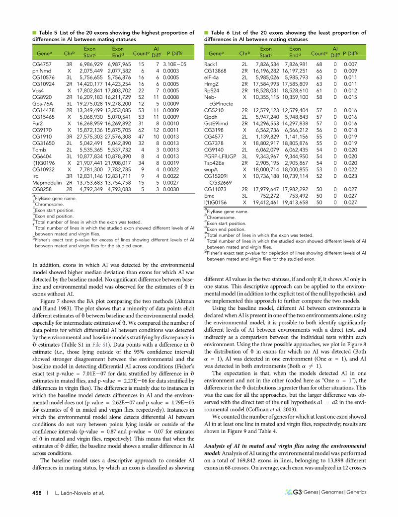
We performed Fisher’s exact test to determine if the proportion oflines showing AI in a given exon was significantly higher (Table 5) orlower (Table 6) than the proportion of lines showing AI for all otherexons. While the environmental approach does not depend on popu-lation frequency of variants, this further analysis does. By searching forexcess (or depletion) of differences in AI across environments in thestudy population, our power depends on the number of exons that canbe tested in the population, and this number is smaller for rare variants.This is especially true for Table 6, where a significant depletion of AIacross environments can be detected only when a large number ofexons (50 or more) have been tested, and none show differences ofAI across environments.

Table 5 lists the 20 genes with the highest excess of lines showingdifferences in AI between mated and virgin flies, according to Fisher’sexact test. These are the genes that show the highest levels of cis byenvironment variation, which suggests regulatory genetic variation inthe response to mating itself.

Table 6 lists the 20 genes showing the least difference in AI betweenmated and virgin flies, according to Fisher’s exact test. These are genesthat show unusually low levels of cis by environment variation, com-pared to other genes in the genome, suggesting robust cis activity.Another possible interpretation is that the allele frequency for differentregulatory alleles in this population is low.

The environmental model can test variation of AI across environ-ments, genotypes, sex, and other conditions. We compared AI levelsbetween the F1’s r365·w1118 and r907·w1118—the two genotypeshaving, respectively, the lower and higher proportion of exons withAI. A total of 406 exons was analyzed in both lines and used for thisanalysis. In mated flies, AI was detected in 16 exons in line r365 and124 in line r907, while in virgin flies, AI was detected in 14 exons in liner365 and 123 in line r907. Difference in AI between r365 and r907 wasdetected in 88 and 83 exons, respectively, or �20%, indicating a largenumber of differences between alleles in these two F1s.

ConclusionsWe present a direct approach for simultaneously testing of AI anddifferences inAIacross environments.Wemeasuredperformanceusingsimulated data, showing that the method has relatively low Type I andType II error rates.Ourmodel alsoaccounts fordifferences inmagnitudeof gene expression counts and unassigned reads, while providing amoreconservative method to estimate AI differences between different en-vironments. Our model protects from increases in type I error evenwhen the number of sequenced reads in the two environments differ by10-fold.We reanalyzed published data to further investigate robustness

of AI to environmental conditions. Our results indicate that gene reg-ulation is substantially robust to environmental changes, with a smallnumber of notable exceptions among genes whose expression is af-fected by mating status. An analysis directly comparing two differentF1s shows�20% of the exons have differences in cis regulation amonglines; this estimate is on par with the detection of cis differences inregulation in the population, and demonstrates that the environmentalmodel can be used to test G·G across F1s as well as G·E effects.

ACKNOWLEDGMENTSThis work was partly financed by the Marie Curie InternationalResearch Staff Exchange Scheme (IRSES) Project “Developing anEuropean American Next Generation Sequencing (NGS) Network(DEANN)” (grant agreement number: PIRSES-GA-2013-612583),by National Institutes of Health (NIH) grant National Institute ofGeneral Medical Sciences (NIGMS) 102227 to L.M.M., and by theEuropean Research Council under the European Union’s SeventhFramework Program (FP7/2007–2013, grant agreement number294780, “Novabreed”). Mention of trade names or commercial productsin this publication is solely for the purpose of providing specific in-formation, and does not imply recommendation or endorsement bythe United States Department of Agriculture (USDA). USDA is an equalopportunity employer. The authors declare no competing interests.

LITERATURE CITEDAigaki, T., and S. Ohba, 1984 Effect of mating status on Drosophila virilis

lifespan. Exp. Gerontol. 19: 267–278.Altman, D. G., and J. M. Bland, 1983 Measurement in medicine: the

analysis of method comparison studies. Stat. 32: 307.Anders, S., and W. Huber, 2010 Differential expression analysis for se-

quence count data. Genome Biol. 11: R106.Brem, R. B., G. Yvert, R. Clinton, and L. Kruglyak, 2002 Genetic dissection

of transcriptional regulation in budding yeast. Science 296: 752–755.Buil, A., A. A. Brown, T. Lappalainen, A. Viñuela, M. N. Davies et al.,

2015 Gene-gene and gene-environment interactions detected by tran-scriptome sequence analysis in twins. Nat. Genet. 47: 88–91.

Castel, S. E., A. Levy-Moonshine, P. Mohammadi, E. Banks, and T. Lappalainen,2015 Tools and best practices for data processing in allelic expressionanalysis. Genome Biol. 16: 195.

Chen, J., V. Nolte, and C. Schlötterer, 2015 Temperature stress mediatesdecanalization and dominance of gene expression in Drosophila mela-nogaster. PLOS Genet. 11: e1004883.

Cohen, J., 1960 A coefficient of agreement for nominal scales. Educ. Psy-chol. Meas. 20: 37–46.

Coffman, C., R. W. Doerge, M. L. Wayne, and L. M. McIntyre,2003 Intersection tests for single marker QTL analysis can be morepowerful than two marker QTL analysis. BMC Genetics 4: 10.

Crowley, J. J., V. Zhabotynsky, W. Sun, S. Huang, I. K. Pakatci et al.,2015 Analyses of allele-specific gene expression in highly divergentmouse crosses identifies pervasive allelic imbalance. Nat. Genet. 47: 353–360.

Cubillos, F. A., O. Stegle, C. Grondin, M. Canut, S. Tisné et al.,2014 Extensive cis-regulatory variation robust to environmental per-turbation in Arabidopsis. Plant Cell 26: 4298–4310.

Degner, J. F., J. C. Marioni, A. A. Pai, J. K. Pickrell, E. Nkadori et al.,2009 Effect of read-mapping biases on detecting allele-specific expres-sion from RNA-sequencing data. Bioinformatics 25: 3207–3212.

Di, Y., D. W. Schafer, J. S. Cumbie, and J. H. Chang, 2011 The NBPnegative binomial model for assessing differential gene expression fromRNA-Seq. Stat. Appl. Genet. Mol. Biol. 10: 1–28.

Edsgärd, D., M. J. Iglesias, S.-J. Reilly, A. Hamsten, P. Tornvall et al.,2016 GeneiASE: detection of condition-dependent and static allele-specific expression from RNA-seq data without haplotype information.Sci. Rep. 6: 21134.

Volume 8 February 2018 | Allelic Imbalance Between Conditions | 459

Everaerts, C., J. P. Farine, M. Cobb, and J. F. Ferveur, 2010 Drosophilacuticular hydrocarbons revisited: mating status alters cuticular profiles.PLoS One 5: e9607.

Fear, J. M., L. G. Leon-Novelo, A. M. Morse, A. R. Gerken, K. Van Lehmannet al., 2016 Buffering of genetic regulatory networks in Drosophilamelanogaster. Genetics 203: 1177–1190.

Graze, R. M., L. M. McIntyre, B. J. Main, M. L. Wayne, and S. V Nuzhdin,2009 Regulatory divergence in Drosophila melanogaster and D. simu-lans, a genome-wide analysis of allele-specific expression. Genetics 183:547–561, 1SI–21SI.

Graze, R. M., L. L. Novelo, V. Amin, J. M. Fear, G. Casella et al.,2012 Allelic imbalance in Drosophila hybrid heads: exons, isoforms, andevolution. Mol. Biol. Evol. 29: 1521–1532.

Graze, R. M., L. M. McIntyre, A. M. Morse, B. M. Boyd, S. V. Nuzhdin et al.,2014 What the X has to do with it: differences in regulatory variabilitybetween the sexes in Drosophila simulans. Genome Biol. Evol. 6: 818–829.

Gregg, C., J. Zhang, B. Weissbourd, S. Luo, G. P. Schroth et al., 2010 High-resolution analysis of parent-of-origin allelic expression in the mousebrain. Science 329: 643–648.

Knowles, D. A., J. R. Davis, H. Edgington, A. Raj, M. J. Favé et al.,2017 Allele-specific expression reveals interactions between geneticvariation and environment. Nat. Methods 14: 699–702.

Kurmangaliyev, Y. Z., A. V. Favorov, N. M. Osman, K.-V. Lehmann, D.Campo et al., 2015 Natural variation of gene models in Drosophilamelanogaster. BMC Genomics 16: 198.

Lawniczak, M. K., and D. J. Begun, 2004 A genome-wide analysis ofcourting and mating responses in Drosophila melanogaster females. Ge-nome 47: 900–910.

León-Novelo, L. G., L. M. McIntyre, J. M. Fear, and R. M. Graze, 2014 Aflexible Bayesian method for detecting allelic imbalance in RNA-seq data.BMC Genomics 15: 920.

León-Novelo, L., C. Fuentes, and S. Emerson, 2017 Marginal likelihoodestimation of negative binomial parameters with applications to RNA-seqdata. Biostatistics 18: 637–650.

Lin, M., A. Hrabovsky, E. Pedrosa, T. Wang, D. Zheng et al., 2012 Allele-biased expression in differentiating human neurons: implications forneuropsychiatric disorders. PLoS One 7: e44017.

Lo, H. S., Z. Wang, Y. Hu, H. H. Yang, S. Gere et al., 2003 Allelic variationin gene expression is common in the human genome. Genome Res. 13:1855–1862.

Maurano, M. T., R. Humbert, E. Rynes, R. E. Thurman, E. Haugen et al.,2012 Systematic localization of common disease-associated variation inregulatory DNA. Science 337: 1190–1195.

McCarroll, S. A., A. Huett, P. Kuballa, S. D. Chilewski, A. Landry et al.,2008 Deletion polymorphism upstream of IRGM associated withaltered IRGM expression and Crohn’s disease. Nat. Genet. 40: 1107–1112.

McGraw, L. A., A. G. Clark, and M. F. Wolfner, 2008 Post-mating geneexpression profiles of female Drosophila melanogaster in response to timeand to four male accessory gland proteins. Genetics 179: 1395–1408.

McManus, C. J., J. D. Coolon, M. O. Duff, J. Eipper-Mains, B. R. Graveleyet al., 2010 Regulatory divergence in Drosophila revealed by mRNA-seq.Genome Res. 20: 816–825.

Moyerbrailean, G. A., A. L. Richards, D. Kurtz, C. A. Kalita, G. O. Davis et al.,2016 High-throughput allele-specific expression across 250 environ-mental conditions. Genome Res. 26: 1627–1638.

Munger, S. C., N. Raghupathy, K. Choi, A. K. Simons, D. M. Gatti et al.,2014 RNA-Seq alignment to individualized genomes improves transcriptabundance estimates in multiparent populations. Genetics 198: 59–73.

R Core Team, 2017 R: A Language and Environment for Statistical Com-puting. R Foundation for Statistical Computing, Vienna, Austria.

Robinson, M. D., and G. K. Smyth, 2007 Small-sample estimation of negativebinomial dispersion, with applications to SAGE data. Biostatistics 9: 321–332.

Rockman, M. V., and G. A. Wray, 2002 Abundant raw material for cis-regulatory evolution in humans. Mol. Biol. Evol. 19: 1991–2004.

Ronald, J., J. M. Akey, J. Whittle, E. N. Smith, G. Yvert et al.,2005 Simultaneous genotyping, gene-expression measurement, anddetection of allele-specific expression with oligonucleotide arrays. Ge-nome Res. 15: 284–291.

Rozowsky, J., A. Abyzov, J. Wang, P. Alves, D. Raha et al., 2011 AlleleSeq:analysis of allele-specific expression and binding in a network framework.Mol. Syst. Biol. 7: 522.

Satya, R. V., N. Zavaljevski, and J. Reifman, 2012 A new strategy to reduceallelic bias in RNA-Seq readmapping. Nucleic Acids Res. 40: e127.

Skelly, D. A., M. Johansson, J. Madeoy, J. Wakefield, and J. M. Akey, 2011 Apowerful and flexible statistical framework for testing hypotheses of allele-specific gene expression from RNA-seq data. Genome Res. 21: 1728–1737.

Stevenson, K. R., J. D. Coolon, and P. J. Wittkopp, 2013 Sources of bias inmeasures of allele-specific expression derived from RNA-sequence dataaligned to a single reference genome. BMC Genomics 14: 536.

Stranger, B. E., S. B. Montgomery, A. S. Dimas, L. Parts, O. Stegle et al.,2012 Patterns of cis regulatory variation in diverse human populations.PLoS Genet. 8: e1002639.

Tung, J., M. Y. Akinyi, S. Mutura, J. Altmann, G. A. Wray et al.,2011 Allele-specific gene expression in a wild nonhuman primatepopulation. Mol. Ecol. 20: 725–739.

Turro, E., S.-Y. Su, Â. Gonçalves, L. J. M. Coin, S. Richardson et al.,2011 Haplotype and isoform specific expression estimation using multi-mapping RNA-seq reads. Genome Biol. 12: R13.

von Korff, M., S. Radovic, W. Choumane, K. Stamati, S. M. Udupa et al.,2009 Asymmetric allele-specific expression in relation to developmentalvariation and drought stress in barley hybrids. Plant J. 59: 14–26.

Wang, M., S. Uebbing, and H. Ellegren, 2017 Bayesian inference of allele-specific gene expression indicates abundant cis-regulatory variation innatural flycatcher populations. Genome Biol. Evol. 9: 1266–1279.

Wittkopp, P. J., B. K. Haerum, and A. G. Clark, 2004 Evolutionary changesin cis and trans gene regulation. Nature 430: 85–88.

Yan, H., W. Yuan, V. E. Velculescu, B. Vogelstein, and K. W. Kinzler,2002 Allelic variation in human gene expression. Science 297: 1143.

Zhang, X., and J. O. Borevitz, 2009 Global analysis of allele-specific ex-pression in Arabidopsis thaliana. Genetics 182: 943–954.

Zhou, S., T. F. C. Mackay, and R. R. H. Anholt, 2014 Transcriptional andepigenetic responses to mating and aging in Drosophila melanogaster.BMC Genomics 15: 927.

Communicating editor: R. W. Doerge

460 | L. León-Novelo et al.