direct frequency comb spectroscopy for optical frequency
TRANSCRIPT

Direct Frequency Comb Spectroscopy for Optical
Frequency Metrology and Coherent Interactions
by
Adela Marian
B.A., University of Bucharest, 1998
A thesis submitted to the
Faculty of the Graduate School of the
University of Colorado in partial fulfillment
of the requirements for the degree of
Doctor of Philosophy
Department of Physics
2005

This thesis entitled:Direct Frequency Comb Spectroscopy for Optical Frequency Metrology and Coherent
Interactionswritten by Adela Marian
has been approved for the Department of Physics
Dr. Jun Ye
Dr. John L. Hall
Date
The final copy of this thesis has been examined by the signatories, and we find thatboth the content and the form meet acceptable presentation standards of scholarly
work in the above mentioned discipline.

iii
Marian, Adela (Ph.D., Physics)
Direct Frequency Comb Spectroscopy for Optical Frequency Metrology and Coherent
Interactions
Thesis directed by Dr. Jun Ye
We take advantage of a phase-stable, wide-bandwidth femtosecond laser to bridge
the fields of high-resolution spectroscopy and ultrafast science. This approach, which we
call Direct Frequency Comb Spectroscopy (DFCS), involves using light from a comb of
appropriate structure to directly interrogate atomic levels and to study time-dependent
quantum coherence. In fact, DFCS may be effectively applied to determine absolute
frequencies for atomic transitions anywhere within the comb bandwidth, obviating the
need for broadly tunable and absolutely referenced continuous-wave (cw) lasers.
In this work, we apply DFCS to determine absolute atomic transition frequencies
for one- and two-photon processes in laser-cooled 87Rb atoms. In addition, DFCS
enables studies of coherent pulse accumulation and multipulse interference, permitted
by the relatively long-lived excited states. These effects are well modeled by our density
matrix theory describing the interaction of the femtosecond comb with the cold atoms.
As in the case of precision spectroscopy performed with cw lasers, the use of
the femtosecond comb as a probe requires a careful understanding of all systematic
effects. We isolate and then mitigate the effects of the dominant sources of systematic
errors, which include the mechanical effect of the optical comb on the atomic motion,
Stark shifts by the probe laser, and Zeeman frequency shifts. The absolute frequency
measurement results are comparable to the highest resolution measurements made with
cw lasers. In addition, by determining the previously unmeasured absolute frequency
of the 5S-7S two-photon transitions in 87Rb, we show that prior knowledge of atomic
transition frequencies is not essential for DFCS.

Dedication
To my family.

Acknowledgements
I would like to offer my gratitude to the people who have made my time here at
JILA profitable and interesting. There are many people who have helped along the way
and I hope I have included all of them below.
Special thanks are due to my advisor Jun Ye who gave me the opportunity to work
on a very new and challenging experiment. Under his guidance I have learned about
cold Rb, laser stabilization, mode-locked lasers and integrating cutting edge techniques
to probe new physics.
I would especially like to thank the people who worked closely with me on the Rb
project within the last two years: Matt Stowe, John Lawall and Daniel Felinto. This
thesis would not have been possible but for their help. I have gained a lot from our
numerous discussions, particularly during John’s three-month visit. In the early stages
of the experiment, I benefited from the involvement and helpful suggestions of Xinye
Xu, Tai Hyun Yoon and Long-Sheng Ma.
My experience here has been made more interesting and fun by the people who
were working on various other experiments in the lab and with me at times, in particular
Joe Berry, Kevin Holman, Seth Foreman, Jason Jones, Tara Fortier, Mark Notcutt
and David Jones. I also enjoyed interacting with and learning interesting things from
members of the fs stabilization group, Kevin Moll, Darren Hudson and Mike Thorpe,
the cold strontium group, Tom Loftus, Andrew Ludlow, Marty Boyd and Tetsuya Ido,
and the cold molecule group, Eric Hudson and Heather Lewandowski.

vi
Thanks are also due to the support staff at JILA, their help over the years was
invaluable. Terry Brown and James Fung-A-Fat deserve double-thanks for the patience
they showed in guiding me through the art of electronics, while Alan Pattee and Hans
Green have always been very helpful in the machine shop.
I wish to thank all of my committee members, Chris Greene, Jan Hall, David
Jonas, Henry Kapteyn and Jun Ye, for their comments. I especially thank Jan for all
of his suggestions and kind encouragement. I greatly appreciate Qudsia Quraishi’s help
in proofreading the final copy of this thesis, as well.
Much thanks to my dear friends Susan Duncan, Peter Schwindt, Anne Curtis,
Phil Kiefer and Malcolm Rickard for making my stay in Boulder both enjoyable and
entertaining.
Finally, I wish to thank my family. My parents, my two sisters and Mike were
always there for me; I thank them for their constant support, love and patience.
vii
Contents
Chapter
1 Introduction 1
1.1 Overview . . . . . . . . . . . . . . . . . . . . . . . . . . . . . . . . . . . 1
1.2 What about using the femtosecond comb directly for spectroscopy? . . . 4
1.3 Time- and frequency-domain description of mode-locked lasers . . . . . 5
1.4 Direct Frequency Comb Spectroscopy . . . . . . . . . . . . . . . . . . . 8
2 Density-matrix method for coherent accumulation
in a multi-level atom 12
2.1 Modeling coherent interactions . . . . . . . . . . . . . . . . . . . . . . . 13
2.1.1 The coherently excited density matrix ρc . . . . . . . . . . . . . 18
2.1.2 The incoherent feeding terms . . . . . . . . . . . . . . . . . . . . 20
2.2 Summary of the coherent interaction model . . . . . . . . . . . . . . . . 22
2.3 Coherent accumulation enables high resolution . . . . . . . . . . . . . . 23
3 Experimental Apparatus: the femtosecond Ti:S setup and the MOT 27
3.1 The femtosecond Ti:S laser and its stabilization setup . . . . . . . . . . 27
3.1.1 Stabilizing the two degrees of freedom of mode-locked lasers . . . 28
3.1.2 Stabilization of the laser repetition rate . . . . . . . . . . . . . . 29
3.1.3 Self-referencing . . . . . . . . . . . . . . . . . . . . . . . . . . . . 31
3.1.4 The ν-to-2 ν prism interferometer . . . . . . . . . . . . . . . . . . 32

viii
3.1.5 Stabilization of the laser offset frequency . . . . . . . . . . . . . . 34
3.2 The MOT . . . . . . . . . . . . . . . . . . . . . . . . . . . . . . . . . . . 36
3.2.1 Diode lasers: description and stabilization . . . . . . . . . . . . . 36
3.2.2 MOT details . . . . . . . . . . . . . . . . . . . . . . . . . . . . . 39
4 Characterization of the systematic effects related to direct frequency comb spec-
troscopy 41
4.1 Doppler-free two-photon transitions with cw and pulsed sources . . . . . 41
4.2 Background for the technique of two-photon DFCS . . . . . . . . . . . . 43
4.3 Experimental method . . . . . . . . . . . . . . . . . . . . . . . . . . . . 46
4.4 Main systematic effects . . . . . . . . . . . . . . . . . . . . . . . . . . . 49
4.4.1 Stability of the reference for the pulse repetition rate . . . . . . . 51
4.4.2 Mechanical action of the probe . . . . . . . . . . . . . . . . . . . 53
4.4.3 AC Stark shift and power broadening . . . . . . . . . . . . . . . 62
4.4.4 Nulling stray magnetic fields . . . . . . . . . . . . . . . . . . . . 64
4.5 Conclusion . . . . . . . . . . . . . . . . . . . . . . . . . . . . . . . . . . 65
5 Two-photon absolute frequency measurements 66
5.1 Scanning fr gives a full spectrum . . . . . . . . . . . . . . . . . . . . . . 67
5.2 Absolute frequency measurements . . . . . . . . . . . . . . . . . . . . . 71
5.3 5S-7S absolute frequency measurements . . . . . . . . . . . . . . . . . . 72
6 One-photon absolute frequency measurements 76
6.1 Detection and timing scheme for the direct 5P measurements . . . . . . 76
6.2 5P3/2 frequency measurements . . . . . . . . . . . . . . . . . . . . . . . 80
6.3 5P1/2 frequency measurements . . . . . . . . . . . . . . . . . . . . . . . 83
7 Summary and outlook 87

ix
Bibliography 90

x
Tables
Table
2.1 Relevant times for the interaction of the femtosecond laser with the
87Rb atoms. . . . . . . . . . . . . . . . . . . . . . . . . . . . . . . . . . . 15
5.1 87Rb level structure from direct frequency comb spectroscopy. . . . . . . 72
6.1 Example of a set of fr and f0 pairs used for the indirect scanning of the
intermediate 5P3/2 F′=3 state. . . . . . . . . . . . . . . . . . . . . . . . 82

xi
Figures
Figure
1.1 Correspondence between the time and frequency domains for a Ti:S
mode-locked laser. . . . . . . . . . . . . . . . . . . . . . . . . . . . . . . 7
1.2 Schematic of the fundamental premise of Direct Frequency Comb Spec-
troscopy (DFCS). . . . . . . . . . . . . . . . . . . . . . . . . . . . . . . . 9
2.1 Cascade configuration for a multi-level atom. . . . . . . . . . . . . . . . 13
2.2 Time evolution of the populations ρ22 and ρ33 for a three-level atom
interacting with a train of hyperbolic-secant pulses. . . . . . . . . . . . . 17
2.3 Vector diagrams for the four terms present in the expression for the sam-
ple Dyson coefficient. . . . . . . . . . . . . . . . . . . . . . . . . . . . . . 20
2.4 Decay paths for the 5D levels of 87Rb. . . . . . . . . . . . . . . . . . . . 21
2.5 Temporal dynamics of the 5D populations, illustrating the interplay of
the two timescales of the system, the excitation and the optical pumping. 24
2.6 Two aspects of coherent pulse accumulation: quadratic increase of the
5D population and linewidth decrease versus the accumulated pulses. . . 26
3.1 Optical layout of the KLM Ti:S laser used in the experiment. . . . . . . 29
3.2 Stabilization diagram used for phase-locking of the laser repetition rate
fr to a stable microwave reference. . . . . . . . . . . . . . . . . . . . . . 30

xii
3.3 Diagram of the ν-to-2 ν prism interferometer used for the detection of the
comb offset frequency. . . . . . . . . . . . . . . . . . . . . . . . . . . . . 33
3.4 Stabilization diagram used for phase-locking of the laser offset frequency
f0 to a stable microwave reference. . . . . . . . . . . . . . . . . . . . . . 35
3.5 Saturated absorption spectra, showing the hyperfine structure of the
5S1/2 → 5P3/2 transitions for the two Rb isotopes. . . . . . . . . . . . . 38
4.1 Schematic of Doppler-free two-photon spectroscopy. . . . . . . . . . . . 42
4.2 Schematic of the 87Rb energy levels participating in the one- and two-
photon transitions, including the wavelength and energy level information. 44
4.3 Resonantly enhanced two-photon transition with detunings from the in-
termediate and excited states. . . . . . . . . . . . . . . . . . . . . . . . . 45
4.4 Timing scheme used for the two-photon measurements. . . . . . . . . . . 47
4.5 Implementation of the setup for the two-photon studies: counterpropa-
gating beams and subsequent PMT detection. . . . . . . . . . . . . . . . 48
4.6 Experimental setup for scanning f0 and typical closed two-photon line-
shape obtained from such a frequency scan. . . . . . . . . . . . . . . . . 50
4.7 Comparison among two-photon lineshapes obtained with different rf ref-
erences for the fr lock. . . . . . . . . . . . . . . . . . . . . . . . . . . . . 52
4.8 Schematic of the detunings from the intermediate and excited states rel-
evant for the radiation pressure studies. . . . . . . . . . . . . . . . . . . 54
4.9 Momentum transferred by the optical frequency comb (in a single probe
beam configuration) to the 87Rb atoms. . . . . . . . . . . . . . . . . . . 55
4.10 Momentum transferred by the fs probe to the atoms: comparison between
the experiment and a simplified theory. . . . . . . . . . . . . . . . . . . 57
4.11 Two-photon signal vs. radial coordinate r for a Gaussian probe beam
profile. . . . . . . . . . . . . . . . . . . . . . . . . . . . . . . . . . . . . . 57
xiii
4.12 Momentum transferred by the fs probe to the atoms: comparison between
the experiment and the more complete theoretical model. . . . . . . . . 58
4.13 Momentum transferred by the fs probe to the atoms: line center shift
and broadening for the single-beam and the counterpropagating-beam
configurations. . . . . . . . . . . . . . . . . . . . . . . . . . . . . . . . . 59
4.14 Time evolution of the 5D fluorescence signal lineshape showing the me-
chanical action of the optical comb for two detunings from the 5P state. 60
4.15 Detailed comparison of the lineshape under the two detuning conditions
after an interaction time of 300 µs. . . . . . . . . . . . . . . . . . . . . . 61
4.16 Schematic of the detunings from the intermediate and excited states rel-
evant for the Stark-shifted data. . . . . . . . . . . . . . . . . . . . . . . 62
4.17 Measurement of the line center frequency and linewidth for the closed
two-photon transition, showing AC Stark and radiation pressure shifts. . 63
4.18 Cancellation of the residual magnetic fields, using the two-photon fluo-
rescence signal. . . . . . . . . . . . . . . . . . . . . . . . . . . . . . . . . 65
5.1 Experimental setup for scanning the laser repetition frequency fr and
resulting two-photon spectrum. . . . . . . . . . . . . . . . . . . . . . . . 68
5.2 Experimental and simulated two-photon spectra obtained with a fre-
quency scan of fr. . . . . . . . . . . . . . . . . . . . . . . . . . . . . . . 70
5.3 Typical 5S1/2 F=2→ 7S1/2 F′′=2 two-photon Lorentzian lineshape ob-
tained from an f0 scan and frequency shift of the transition line center
versus probing time. . . . . . . . . . . . . . . . . . . . . . . . . . . . . . 74
6.1 Detection assembly for the direct one-photon measurements. . . . . . . . 77
6.2 Timing scheme for the direct one-photon measurements. . . . . . . . . . 78
6.3 Schematic of one- and two-photon DFCS, used for measuring single-
photon transition frequencies. . . . . . . . . . . . . . . . . . . . . . . . . 79

xiv
6.4 Lineshapes of the 5S1/2 F=2→ 5P3/2 F′=3 transition, obtained from one-
and two-photon DFCS. . . . . . . . . . . . . . . . . . . . . . . . . . . . . 81
6.5 Theoretical plot of the time evolution of the ground state populations for
two symmetric detunings from the 5P3/2 F′=3 state. . . . . . . . . . . . 82
6.6 Lineshapes of the 5S1/2 F=2→ 5P1/2 F′=2 transition, obtained from one-
and two-photon DFCS. . . . . . . . . . . . . . . . . . . . . . . . . . . . . 83
6.7 Theoretical plot of the time evolution of the ground state populations for
two symmetric detunings from the 5P1/2 F′=2 state. . . . . . . . . . . . 84
6.8 Raw and normalized data for the 5S1/2 F=2→ 5P1/2 F′=2 transition,
obtained from two-photon DFCS. . . . . . . . . . . . . . . . . . . . . . . 85

Chapter 1
Introduction
1.1 Overview
The recent introduction [1,2] of phase-stabilized, wide-bandwidth frequency combs
based on mode-locked femtosecond (fs) lasers has provided optical frequency markers
that may be directly linked to optical or microwave standards. Many laboratories
have since constructed frequency combs for a variety of exciting applications. These in-
clude: measurements of absolute optical frequencies and precision laser spectroscopy [3],
development of optical atomic clocks [4, 5], optical frequency synthesis [6] and broad-
band, phase-coherent spectral generation [7,8], along with coherent synthesis of optical
pulses [9], phase-sensitive extreme nonlinear optics [10] and pulse timing stabilization.
Ultrashort pulses may also be applied to study coherent evolution in atomic and
molecular systems. In particular, coherent wave packet motion has been observed and
even actively controlled [11]. In addition, current work involves the use of fs lasers to
achieve quantum coherent control in semiconductors [12] and in studying the temporal
dynamics of biological physics [13]. These studies may require pulses which are tailored
to probe or indeed selectively drive the dynamical process. This necessitates precise
control over the amplitude- and phase of the ultrashort pulses, otherwise known as
optical pulse synthesis [14].
On the road to tailoring optical pulses, one powerful demonstration was the phase-
coherence established between two independent femtosecond lasers. Coherent optical

2
pulse synthesis from two fs lasers has been reported in 2001 [9], where light pulses were
generated with durations shorter than those obtainable from the individual lasers. This
leads to an extended coherent bandwidth to be used in ultrafast experiments.
Before the advent of phase-stabilization, research showed [15] that the longitudinal
modes of a 73-fs Kerr-lens mode-locked Ti:S laser [16] are uniformly distributed in
frequency space within an experimental resolution of better than 10−16 and that the
mode spacing differs from the pulse repetition frequency by less than 10−15. Thus,
passively mode-locked Ti:S lasers can possess an inherent stability and that is one of
their most powerful features.
On an apparently independent path, precise spectroscopic studies of atoms and
molecules have always been performed with continuous wave (cw) lasers, refined over
the years to be very narrow spectrally, in order to enable probing of very narrow fea-
tures [17]. Precision atomic and molecular spectroscopy, enabled by the progress in
cw laser stabilization, has been one of the most important fields of modern scientific
research, providing the experimental underpinning of quantum mechanics and quantum
electrodynamics (e.g. detailed investigations of atomic and molecular structure, deter-
mination of fundamental constants, realization of time, frequency and length standards,
tests of special relativity, progress in optical communications etc.).
In the first experiments using mode-locked femtosecond lasers, they served only as
rulers for studying atomic systems and did not directly interrogate the atoms. Hansch
and coworkers used the comb spectrum of a fs laser to span an optical interval of 50 nm,
and improved the measurement accuracy of the D1 resonance line in cesium by almost
three orders of magnitude [18], providing a new value for the fine structure constant. To
measure the D1 line, its frequency was compared against the fourth harmonic of a CH4-
stabilized laser employed as the absolute frequency reference. The fs comb was used
as a frequency ruler to measure the resulting frequency difference of 18.39 THz (this
frequency interval contained roughly 244 000 comb lines). To uniquely determine the
3
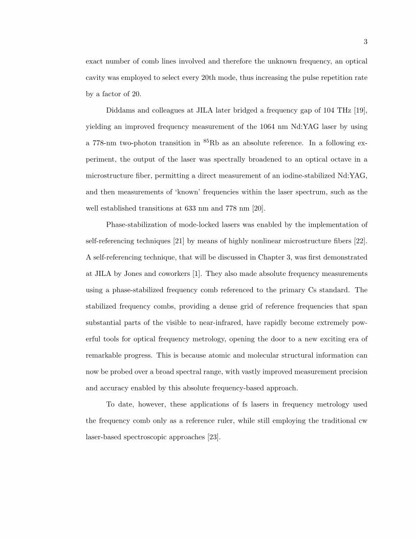
exact number of comb lines involved and therefore the unknown frequency, an optical
cavity was employed to select every 20th mode, thus increasing the pulse repetition rate
by a factor of 20.
Diddams and colleagues at JILA later bridged a frequency gap of 104 THz [19],
yielding an improved frequency measurement of the 1064 nm Nd:YAG laser by using
a 778-nm two-photon transition in 85Rb as an absolute reference. In a following ex-
periment, the output of the laser was spectrally broadened to an optical octave in a
microstructure fiber, permitting a direct measurement of an iodine-stabilized Nd:YAG,
and then measurements of ‘known’ frequencies within the laser spectrum, such as the
well established transitions at 633 nm and 778 nm [20].
Phase-stabilization of mode-locked lasers was enabled by the implementation of
self-referencing techniques [21] by means of highly nonlinear microstructure fibers [22].
A self-referencing technique, that will be discussed in Chapter 3, was first demonstrated
at JILA by Jones and coworkers [1]. They also made absolute frequency measurements
using a phase-stabilized frequency comb referenced to the primary Cs standard. The
stabilized frequency combs, providing a dense grid of reference frequencies that span
substantial parts of the visible to near-infrared, have rapidly become extremely pow-
erful tools for optical frequency metrology, opening the door to a new exciting era of
remarkable progress. This is because atomic and molecular structural information can
now be probed over a broad spectral range, with vastly improved measurement precision
and accuracy enabled by this absolute frequency-based approach.
To date, however, these applications of fs lasers in frequency metrology used
the frequency comb only as a reference ruler, while still employing the traditional cw
laser-based spectroscopic approaches [23].
4
1.2 What about using the femtosecond comb directly for spec-
troscopy?
The main problem with using a pulsed laser for spectroscopy is the broad fre-
quency bandwidth associated with a short pulse. The broad spectrum prevents high-
precision measurements of state energies. This problem can be avoided by using a train
of phase-coherent pulses, which permits frequency resolution orders of magnitude better
than that associated with a single pulse.
T. Hansch first introduced the idea of using coherent pulse trains from mode-
locked lasers for the measurement of optical frequency intervals and high-resolution
spectroscopy in 1976 [24]. A stable train of pulses forms a regular and discrete set of
modes separated by the pulse repetition rate in the frequency domain. Hansch showed
that a sequence of pulses results in signal enhancement over single-pulse excitation for
the atomic transition amplitude. In particular, he pointed out the resonant excitation
probability is proportional to the squared number of pulses arriving within the atomic
lifetime (for small incident light intensities).
The spectroscopic applications of this multi-pulse interference were experimen-
tally demonstrated within the following two years. First, a train of phase-coherent pulses
produced externally to the laser, by multiple reflections of a single pulse injected into an
optical resonator, was utilized for Doppler-free two-photon excitation in Na [25]. Then,
in 1978, the comb of a mode-locked picosecond dye laser [26] was used to measure the
Na 4d fine-structure splitting, i.e. frequency intervals of ∼ 1 GHz, via Doppler-free two-
photon spectroscopy [27]. In this experiment, the axial mode separation was actively
controlled in the frequency domain (equivalent to stabilizing the repetition frequency of
a train of pulses). As the laser spectrum is scanned, resonant excitation occurs whenever
the sum of two frequencies is equal to the two-photon transition frequency. The comb
of lines was used as a ruler in frequency space to measure optical frequency differences.

5
The limitation of this technique was the small bandwidth of the available mode-locked
dye lasers, preventing measurements of large optical frequency differences.
The powerful combination of cw stabilization, passively mode-locked lasers and
microstructure fibers, culminating with the phase-stabilization of femtosecond lasers,
has made it possible to meet some of the conditions necessary to probe atomic structure
directly with a frequency comb for precise frequency measurements: (i) short pulses,
i.e. wide bandwidth (ii) pulse-to-pulse coherence and (iii) absolute referencing of the
frequency comb.
Many new technologies have been enabled by the phase-stabilization of femtosec-
ond lasers. In order to be able to phase-stabilize a femtosecond laser, one needs to
understand its pulse characteristics. The connection between the short pulses emitted
from the laser and the powerful frequency comb generated is described in the following
section.
1.3 Time- and frequency-domain description of mode-locked lasers
The output of a mode-locked laser is a very regular train of ultrashort pulses, with
the interval between pulses τ usually ∼ 6 orders of magnitude higher than the pulse
duration. These short pulses are produced when a fixed phase relationship is established
among all the lasing longitudinal modes of the laser cavity (i.e. mode-locking), resulting
in their coherent addition and the formation of a light pulse. An isolated light pulse
can be represented as a sinusoidal optical carrier of angular frequency ωc, amplitude-
modulated by an envelope function E(t), with the electric field thus given by E(t) =
E(t) exp [ i (ωc t + φ0)]. When traveling through a medium, the carrier propagates at
the phase velocity, while the envelope advances at the group velocity. In general, the
two velocities are different for a dispersive medium: vp = c /n and vg = c /(n + ω ∂ n
∂ ω
).
For instance, traversing a distance l in a dispersive material gives a phase shift of
ωc
(l
vg− l
vp
)= l ωc
2
c∂ n∂ ω = −2π l ∂ n
∂ λ . This difference in the phase and group velocities

6
inside the laser cavity causes the phase between the optical carrier and the peak of the
envelope to evolve between successive pulses in the train. Let δφ denote the amount by
which the carrier-envelope phase changes from pulse to pulse. After including this pulse-
to-pulse phase-shift, the electric field of a train of pulses for a fixed spatial coordinate
is
E(t) =∑n
En(t− nτ) exp [ i (ωc t + φ0 − n ωc τ + n δφ)]. (1.1)
By taking its Fourier Transform [28] we obtain the following expression for the angular
frequencies
ωN =N 2π
τ− δφ
τ. (1.2)
Thus, the spectrum of the mode-locked femtosecond laser consists of a wide comb
of discrete optical frequencies, offset from the exact harmonics of the repetition rate
by a frequency proportional to the pulse-to-pulse carrier-envelope phase shift [Fig. 1.1].
The spectrum is described by the simple relation νN = Nfr + f0, where N is a large
integer on the order of 106, fr = 1τ is the pulse repetition rate and f0 = − 1
2π δφ fr is the
carrier-envelope offset frequency. Note that the relevant quantity here is δφ modulo 2π,
i.e. f0 is bounded by fr.
The two laser parameters are dynamic quantities, sensitive to environmental per-
turbations affecting the laser cavity. Not surprisingly, there are no locking mechanisms
between the pulse envelope and the optical carrier inside an unstabilized laser, so their
relative phase δφ experiences fluctuations between successive pulses. Consequently, for
spectroscopic studies with a femtosecond laser, both comb parameters fr and f0 need
to be actively stabilized.
As a reminder, absolute optical frequency measurements are made with respect
to the ground state hyperfine splitting in 133Cs at 9.192631770 GHz, which provides
the current definition for the second. This leap from the optical to the radio-frequency
domain has been a daunting task in frequency metrology for the last 30 years, before

7
fo
fr
νN = N fr + fo
I(ν
ν
)
FT1 fr = τ
E(t
t
φδ φ2δ)
Figure 1.1: Correspondence between the time and frequency domains for a Ti:S mode-locked laser. In the time domain, the carrier-envelope phase changes at a defined ratebetween successive pulses in the train. In the frequency domain, the comb lines arespaced by the laser repetition rate fr and the comb is shifted from integer multiples offr by an offset frequency f0. The Ti:S laser used in the experiment is centered at 778nm and has a FWHM bandwidth of ∼ 55 nm.

8
the introduction of the mode-locked approach. Because of the complexity involved,
only a few harmonic frequency chains were ever implemented, for very specific optical
frequency measurements. A few examples are: the 88 THz transition in CH4 [29] (which
led to the speed of light measurement [30]), the I2-stabilized He-Ne transition at 473
THz [31], the 455 THz intercombination transition in 40Ca [32], the 5s 2S1/2→ 4d 2D5/2
transition at 445 THz in 88Sr+ [33], the 2S-12D transitions in hydrogen and deuterium
at 799 THz [34]. Stabilized frequency combs allow one to phase-coherently link any
unknown optical frequency within the comb spectrum directly to a primary microwave
standard.
1.4 Direct Frequency Comb Spectroscopy
Following our own theoretical studies [35], we take advantage of the phase-stable,
wide-bandwidth femtosecond pulse train to bridge the fields of high-resolution spec-
troscopy and ultrafast science, in a spectroscopic study of laser-cooled 87Rb atoms.
This approach, which we call Direct Frequency Comb Spectroscopy (DFCS), involves
using light from a comb of appropriate structure to directly interrogate atomic levels
and to study time-dependent quantum coherence.
By utilizing a stabilized fs comb, multiple atomic states may be simultaneously
and directly excited, by tuning the appropriate comb lines into resonance, and the subse-
quent dynamics may be probed. Furthermore, given that the comb has two independent
degrees of freedom, it is always possible to simultaneously satisfy two-photon as well as
one-photon resonance conditions.
In fact, DFCS may be applied to determine absolute frequencies for atomic tran-
sitions anywhere within the comb bandwidth. The entire transition spectrum can be
efficiently retrieved by a quick scan of the laser repetition frequency. This obviates the
need for a broadly tunable and absolutely referenced cw laser and is especially useful in
the study of multi-photon processes where several laser sources may be required. Thus,

9
optical frequency combs are a highly efficient tool for precise studies of atomic structure.
In this work, we apply DFCS to determine absolute atomic transition frequencies
for one- and two-photon processes, as illustrated in Fig. 1.2. DFCS enables studies
of coherent pulse accumulation and multipulse interference, permitted by the relatively
long-lived 5D and 7S states. The observed coherent pulse accumulation and interference
effects are well modeled by our density matrix theory describing the interaction of the
femtosecond comb with the atoms, as discussed in Chapter 2. We use the theory results
to construct transition spectra to compare against the experimental spectra.
ν
5D or 7S
5P1/2 or 5P3/2(27 ns)
(240 ns or 88 ns)
5S
3 >
2 >
1 >
f =100 MHzr
87Rb
Figure 1.2: Schematic of the 87Rb energy levels participating in the 5S-5D and 5S-7Stwo-photon transitions and 5S-5P one-photon transitions. These are the relevant levelsprobed using direct frequency comb spectroscopy (DFCS).
We present the details of the implementation of the femtosecond stabilization
scheme and the MOT setup in Chapter 3. These are integrated together for spectro-
scopic studies in Chapter 4.
As in the case of precision spectroscopy performed with cw lasers, the use of the
femtosecond comb as a precision probe requires a careful understanding of all systematic
effects. We find that the dominant effects are the mechanical effect of the optical comb

10
on the atomic motion, the light shift by the probe laser, and the Zeeman frequency
shifts. In Chapter 4, we address the mechanical action of the probe laser by using a
counterpropagating beam configuration. We observe Stark shifts generated by detunings
from the intermediate states in the two-photon processes and we reduce their effect by
always probing on resonance with the intermediate state of interest.
We first study the 5S-5D two-photon transitions in 87Rb, leading to high-resolution
spectroscopy for some of the transitions, as presented in Chapter 5. The measurement
results are comparable to the highest resolution measurements made with cw lasers.
By determining the previously unmeasured absolute frequency of the 5S-7S two-photon
transitions in 87Rb, we show that prior knowledge of atomic transition frequencies is
not essential for this technique to work, and indicate that it can be applied in a broad
context. When resonant enhancement is enabled by a comb component tuned near an
intermediate 5P state, we observe two-photon transitions occurring between initial and
final states that differ by one unit of the total angular momentum (∆F = ±1), which
are absent for far-detuned intermediate states. This capability of accessing adjacent
excited hyperfine levels from the same ground state allows for direct measurements of
hyperfine splittings.
We then use DFCS to measure one-photon transitions, and choose the 5S-5P
transitions as an example, as detailed in Chapter 6. The measurement of 5P states
is also carried out indirectly via the 5S-5D two-photon transitions, by studying their
resonant enhancement when comb components are scanned through the intermediate
5P states. We compare the 5P measurements obtained via one-photon and two-photon
DFCS and clearly demonstrate the importance of population transfer in working with
multilevel systems probed by multiple comb components. Incoherent processes such as
optical pumping govern the population dynamics beyond the atomic decoherence time.
For the case of the indirect 5P frequency measurements via the 5S-5D two-photon
transitions, the experimental data do not yield directly the lineshape. In this case, we

11
use the theory prediction to adjust the raw data and retrieve a Lorentzian lineshape, as
described in Chapter 6.
The optical coherence of a phase-stabilized pulse train provides a spectral re-
solving power approaching that of state-of-the-art cw lasers. At the same time, the
narrow linewidth of individual comb lines permits a precise and efficient determination
of the global energy-level structure, providing a direct connection among the optical,
terahertz, and radio-frequency domains.

Chapter 2
Density-matrix method for coherent accumulation
in a multi-level atom
We will now study coherent accumulation in a multi-level atom interacting with
a train of ultrashort pulses. For the situation where the atomic relaxation times are
longer than the interpulse interval τ , the atomic coherence will survive between two
consecutive pulses, leading to coherent accumulation of excitation in the sample. Con-
structive/destructive interference among the coherences excited by the train of pulses
will determine the final atomic populations. We will focus on the accumulative effects
occurring in the sequential 5S-5P-5D two-photon transitions.
The interaction of the femtosecond comb with the atoms is modeled starting with
the Liouville equation for the density matrix of all the atomic states in the laser band-
width accessible through two-photon absorption, with radiative relaxation included via
phenomenological decay terms. The density matrix equations are solved to a fourth-
order perturbative expansion in the electric field. With the approximation of impulsive
optical excitation during the pulse, followed by free evolution and decay, an iterative nu-
merical procedure is used to determine the state of the atomic system after an arbitrary
number of pulses.

13
3k>
2j >
1i>
5D
5P
5S
k = 1,8
i = 1,2
j = 1,6
Figure 2.1: Cascade configuration for a multi-level atom.
2.1 Modeling coherent interactions
Consider an electric field E(t) interacting with a multi-level atom in which all
the levels are distributed in three different manifolds |1i〉, |2j〉 and |3k〉, in a cascade
configuration, as presented in Fig. 2.1. Here ‘1’ labels the ground 5S states, ‘2’ the
intermediate 5P states and ‘3’ the excited 5D states, while i, j and k stand for the
various fine and hyperfine levels of a specific state. We adopted this simplified notation
for the energy levels only in the theory chapter, because it will make the following
equations easier to follow.
The Hamiltonian of the system H is given by the sum of the field-free atomic
Hamiltonian H0 and the interaction potential between the atom and the electric field
in the electric-dipole approximation Hint. Thus, H = H0 + Hint, with
H0 =∑
i
E1i|1i〉〈1i|+∑j
E2j |2j〉〈2j|+∑k
E3k|3k〉〈3k| and
Hint = −∑i,j
µ1i,2j E(t)|1i〉〈2j|+∑j,k
µ2j,3k E(t)|2j〉〈3k|+ h.c., (2.1)
where E1i, E2j , E3k are the energies of levels |1i〉, |2j〉 and |3k〉, respectively, and µi,j
is the dipole moment of the i → j transition.

14
We are interested in the time evolution of the state of the system after a long
sequence of pulses. This temporal evolution is described by the Bloch equations, derived
from the Liouville equations upon inclusion of the relaxation terms. The starting point
is therefore the Liouville equation for the density-matrix elements of the multi-level
atomic system, resulting in 9 families of equations for the ground-, intermediate- and
excited-state populations, the intra-ground-, intra-intermediate- and intra-excited-state
coherences, as well as the 1-2, 2-3 and 1-3 coherences. For clarity, I will write out
some representative Liouville equations, for the ground-state populations, ground-state
coherences and the 1-2 coherences, respectively:
∂ρ1i,1i
∂t= − i
h〈1i|[H, ρ]|1i〉 ground-state population
∂ρ1i,1s
∂t= − i
h〈1i|[H, ρ]|1s〉, s 6= i intra-ground-state coherence
∂ρ1i,2j
∂t= − i
h〈1i|[H, ρ]|2j〉 1-2 coherence. (2.2)
The 6 remaining families can be written in a similar manner.
The Bloch equations are obtained from the Liouville equations after including the
relaxation rates Γi,j of the (i, j) density matrix components. Note that for our case,
Γ1i,1i = 0, all the population decay rates for a given state are equal, i.e. Γ2j,2j = Γ5P ≡
Γ2 and Γ3k,3k = Γ5D ≡ Γ3, and Γi,j = 12 (Γi,i + Γj,j). The subscripts indicating the
states in the Γ coefficients will all be kept in the following derivation, for symmetry of
the equations. As an example, I will write the Bloch equation for the 1-2 coherence:
∂ρ1i,2j
∂t= −iω1i,2j ρ1i,2j −
i
h〈1i|[Hint, ρ]|2j〉 − Γ1i,2j ρ1i,2j (2.3)
This was obtained by substituting the expression for the Hamiltonian H in Eq. 2.2, with
ωi,j ≡ (Ei−Ej)/h. All the coherence equations look the same as Eq. 2.3, with only the
appropriate change of indices.
Before writing expressions for the populations of levels |1〉 and |2〉, we must also
consider the incoherent feeding of level |2〉 by level |3〉 and |1〉 by |2〉 present in a multi-

15
level atomic system. Including these additional terms gives the populations as
∂ρ1i,1i
∂t= − i
h〈1i|[Hint, ρ]|1i〉 − Γ1i,1i ρ1i,1i +
∑r
γ1i,r ρr,r (2.4)
∂ρ2j,2j
∂t= − i
h〈2j|[Hint, ρ]|2j〉 − Γ2j,2j ρ2j,2j +
∑r
γ2j,r ρr,r
∂ρ3k,3k
∂t= − i
h〈3k|[Hint, ρ]|3k〉 − Γ3k,3k ρ3k,3k.
More details about deriving the incoherent feeding terms will be given in 2.1.2.
We can now integrate Eqs. 2.3 and 2.4, with the assumption of impulsive optical
excitation during the interaction time: the pulse duration is ultrashort compared to the
pulse repetition period or any relaxation time of the system, as seen from Table 2.1.
Pulse duration ∼ 30 fsLaser repetition period 10 ns
5P lifetime 27 ns [36]5D lifetime 240 ns [36]
1-2 coherence lifetime 54 ns1-3 coherence lifetime 480 ns2-3 coherence lifetime 48.5 ns
Table 2.1: Relevant times for the interaction of the femtosecond laser with the87Rb atoms.
This means that the interaction potential Hint changes on a very fast timescale
compared to the Γi,j relaxation rates, allowing us to neglect the temporal dependence
on Γi,j inside the integrals containing Hint, and yielding:
ρ1i,1i(t) = e−Γ1i,1i t
[ρ01i,1i −
i
h
∫ t
0dt′〈1i|[Hint, ρ]|1i〉+
∑r
γ1i,r
∫ t
0dt′eΓ1i,1i t′ ρr,r(t′)
]
ρ1i,2j(t) = e−iω1i,2j t−Γ1i,2j t[ρ01i,2j −
i
h
∫ t
0dt′eiω1i,2j t′〈1i|[Hint, ρ]|2j〉
](2.5)
for the ground-state population and 1-2 coherence, respectively.
Numerical integration of Eq. 2.5 gives the time evolution of the system with ar-
bitrary initial conditions, but is computationally challenging for the 87Rb atom, where
there are two 5S initial levels, six 5P intermediate levels and eight 5D final levels,

16
leading to a total of 162 = 256 coupled Bloch equations. To avoid the long computa-
tional times, our collaborator Daniel Felinto [37,38] has developed an iterative numerical
procedure that determines the state of the atomic system after any number of pulses.
As previously mentioned, for laser repetition periods τ shorter than the relaxation times
of the system, as is the case of 87Rb, the atomic sample will accumulate excitation in
the form of population and coherence.
In Daniel Felinto’s iterative solution, the state of the system before the (n + 1)-
th pulse in the train is obtained from the state prior to the n-th pulse. The relation
connecting ρn+1 to ρn is easily derived from Eq. 2.5 by setting t = τ . Again, making
the impulsive optical excitation assumption means setting t → ∞ in all the integrals
containing Hint; the lower limit can be made t → −∞, since E(t) = 0 for t < 0. For
the two sample elements of the density matrix appearing in Eq. 2.5 we obtain
ρn+11i,1i = e−Γ1i,1iτ
[ρc1i,1i +
∑r
γ1i,r
∫ τ
0dt′eΓ1i,1i t′ ρr,r(t′)
](2.6)
ρn+11i,2j = e−iω1i,2jτ−Γ1i,2jτ
[ρc1i,2j
],
where
ρcr,s = ρn
r,s −i
h
∫ ∞
−∞dt′eiωr,s t′〈r|[Hn
int, ρ]|s〉 (2.7)
is the density matrix coherently excited by the n-th pulse (Hnint), a function of the initial
state prior to the n-th pulse ρn. Expressions similar to Eq. 2.6 are derived for the 7
remaining families of equations.
As a demonstration, Fig. 2.2 (adapted from Felinto et al., reference [38]) shows
the temporal evolution of the ρ22 and ρ33 populations in a three-level atom interacting
with a train of hyperbolic-secant pulses. The total number of coupled Bloch equations
for this system is 32 = 9, so a direct numerical integration is not yet computationally
intensive. The solid lines are a result of the direct numerical integration (∼ 1.5 hours of
computational time), while the open circles arise from successive applications of Eq. 2.6
to the atom initially in the ground state (< 10 s). The transient behavior of the excited

17
level populations is governed by their significantly different (factor of 10) lifetimes, as
demonstrated by the different timescales in the two frames of the figure.
Figure 2.2: (adapted from reference [38]) Time evolution of the populations ρ22 andρ33 for a three-level atom interacting with a train of hyperbolic-secant pulses. The twoframes are different timescales of the same evolution, where the solid lines are a resultof direct numerical integration of the Bloch equations and the open circles come fromsuccessive applications of Eq. 2.6.
After a large number of pulses, the system reaches a stationary state that repeats
every τ . The shape of the direct-integration curve accounts for the very fast change
in population during the pulse interaction time, followed by a slow decay in between
pulses. The numerical-iteration method agrees well with the direct integration, in that
it always matches the value at the minimum. This happens because, in the iteration

18
procedure, the initial state is always taken to be the state ρn just before the impulsive
excitation. The situation would be reversed and the two curves would match at the
maximum if the initial state were the state immediately after each individual pulse.
To summarize, in the simplified treatment of coherent accumulation for a two-
photon process in a multi-level atom, there are two major steps: the first is obtaining the
state of the system after the interaction with a pulse in the train, for an arbitrary initial
state of the atom (Eq. 2.6). The second step is the successive application of Eq. 2.6,
yielding the atomic state after a sequence of pulses, or in other words, describing the
time evolution of the system.
2.1.1 The coherently excited density matrix ρc
There are two quantities left to calculate now, the coherently excited density
matrix in Eq. 2.7, associated with the impulsive excitation during the laser pulse, and
the feeding terms in Eq. 2.4, arising from incoherent decay.
We will first focus on ρc, realizing that it is a product of two probability amplitudes
in the interaction picture
ρci,j = Ci × C∗
j , Ci = 〈i|UI(t)|Ψ0〉, (2.8)
with Ψ0 the initial state of the system, which is a superposition of all the atomic states,
and UI(t) the time propagation operator in the interaction picture, given by
UI(t) = 1 +(− i
h
)∫ t
0dt′HI
int(t′) +
(− i
h
)2 ∫ t
0dt′∫ t′
0dt′′HI
int(t′)HI
int(t′′) + . . . (2.9)
After inserting the relation for HIint(t), HI
int(t) = eiH0t/h Hint(t) e−iH0t/h, and specifying
the electric field E(t) = E(t)eiωct+iφ0 + c.c. as defined in section 1.3, we obtain the
following general expressions for the three groups of probability amplitudes:
C3k(t) =∑s
A3k,3sC03s +
∑j
A3k,2j e−iφ0C02j +
∑i
A3k,1i e−2iφ0C0
1i (2.10)

19
C2j(t) =∑k
A2j,3k eiφ0C03k +
∑s
A2k,2sC02s +
∑i
A2j,1i e−iφ0C0
1i
C1i(t) =∑k
A1i,3k e2iφ0C03k +
∑j
A1i,2j eiφ0C02j +
∑s
A1i,1sC01i,
where Ai,j are the Dyson coefficients corresponding to the time evolution from state i
to state j. This yields the final formula for any element (i, j) of the impulsively excited
density matrix ρc
ρci,j = e−iBi,j φ0
∑r,s
Ai,rA∗j,s eiBr,s φ0ρ0
r,s, (2.11)
with Bi,j = 2∑
k(δ3k,i − δ3k,j) +∑
k(δ2k,i − δ2k,j), where the δ s are Kronecker symbols.
We are interested in developing a theory in the weak-field regime: from the infinite
Dyson series only the terms up to the fourth order in the electric field will be kept. The
fourth order is the smallest order contributing to population in the most excited level
for two-photon transitions from the ground state. In this regime, making the rotating-
wave approximation will result in expressions for the 9 groups of elements Ai,j present
in Eqs. 2.10 and 2.11. As an example, I will write out the expression for A3k,3s:
A3k,3s = δ3k,3s +(− iea0
h
)2∑r
m3k,2rm2r,3s
∫ t
0dt′∫ t′
0dt′′eiδ3k,2r t′eiδ2r,3s t′′E∗(t′)E(t′′)
+(− iea0
h
)4 ∑r,n,q
m3k,2rm2r,1nm1n,2qm2q,3s
∫ t
0dt′∫ t′
0dt′′∫ t′′
0dt′′′∫ t′′′
0dt′′′′eiδ3k,2r t′
× eiδ2r,1n t′′eiδ1n,2q t′′′eiδ2q,3s t′′′′E∗(t′)E∗(t′′)E(t′′′)E(t′′′′) +(− iea0
h
)4
×∑r,n,q
m3k,2rm2r,3nm3n,2qm2q,3s
∫ t
0dt′∫ t′
0dt′′∫ t′′
0dt′′′∫ t′′′
0dt′′′′eiδ3k,2r t′eiδ2r,3n t′′
× eiδ3n,2q t′′′eiδ2q,3s t′′′′E∗(t′)E(t′′)E∗(t′′′)E(t′′′′), (2.12)
with δi,j ≡ ωi,j − ωc the detunings relative to the carrier frequency, mi,j = µi,j/ea
dimensionless dipole moments, e the electron charge and a the Bohr radius. The last
three terms in Eq. 2.12 are second-order and fourth-order contributions to the excitation,
related to the processes of absorption and stimulated emission on the lower and upper
transitions. They are schematically drawn in Fig. 2.3.
This messy expression can be greatly simplified if we consider the situation where

20
2>
3>
1>
Figure 2.3: Vector diagrams for the four terms present in Eqs. 2.12 and 2.13 for thesample Dyson coefficient.
the pulse is ultrashort compared to the time variation determined by the atomic detun-
ings, i.e. we neglect all the exponentials in Eq. 2.12, and if we limit ourselves to the
reasonable case of a real envelope function. Under these approximations, the nested
integrals take a much simpler form, via successive integration by parts, with the result
A3k,3s = δ3k,3s −θ 2
2!
∑r
m3k,2rm2r,3s + (2.13)
+θ 4
4!
(∑r,n,q
m3k,2rm2r,1nm1n,2qm2q,3s +∑r,n,q
m3k,2rm2r,3nm3n,2qm2q,3s
).
Here θ is the pulse area, defined as
θ =ea
h
∫ ∞
−∞dt E(t) pulse area. (2.14)
2.1.2 The incoherent feeding terms
There are two very different timescales over which the populations present in
the feeding-term integrals vary: first, there is a very fast change in population during
the pulse interaction time, followed by a slow, incoherent decay during the interpulse
interval. In this model, it is assumed for simplicity that level |2〉 is fed only by level |3〉,
and |1〉 is only fed by |2〉. Note that the population in the latter level varies in time
due to feeding from |3〉. However, in reality, there are two decay channels for the 5D
population [36], as illustrated in Fig. 2.4: the first is the 5D-5P-5S radiative cascade

21
and the second is the 5D-6P-5S cascade. In fact, we experimentally determine the 5D
population by detecting the 420 nm blue fluorescence emitted in the 6P-5S transition.
The 6P state is not included in the simulation.
5P3/2 (1/2)
6P3/2 (1/2)
776 (762) nm
780 (795) nm 420 (422) nm
62% 38%
31% (27%)
5D
5S
5.2 µm
Figure 2.4: Decay paths for the 5D levels of 87Rb, with the corresponding transitionwavelengths and branching ratios specified. In the experiment, we detect the 6P-5S bluephotons at 420 nm, which represent roughly 10% of the 5D population. The 6P levelsalso decay to the 6S and 4D levels, not pictured here.
For the situation where the pulse duration is ultrashort compared to the laser
repetition period τ and considering only the 5P decay channel for the 5D population,
we have:
∑k
γ2j,3k
∫ τ
0dt′eΓ2j,2j t′ρ3k,3k(t′) '
∑k
γ2j,3k ρc3k,3k
∫ τ
0dt′eΓ2j,2j t′e−Γ3k,3k t′
=∑k
γ2j,3k ρc3k,3k
1− e(Γ2j,2j−Γ3k,3k)τ
Γ3k,3k − Γ2j,2j
(2.15)
∑j
γ1i,2j
∫ τ
0dt′eΓ1i,1i t′ρ2j,2j(t′) '
∑j
γ1i,2j
∫ τ
0dt′eΓ1i,1i t′e−Γ2j,2j t′
×[
ρc2j,2j +
∑k
γ2j,3k
∫ t′
0dt′′eΓ2j,2j t′′ρ3k,3k(t′′)
]
=∑j
γ1i,2j ρc2j,2j
1− e(Γ1i,1i−Γ2j,2j)τ
Γ2j,2j − Γ1i,1i+∑j
∑k
γ1i,2jγ2j,3k
Γ2j,2j − Γ3k,3k
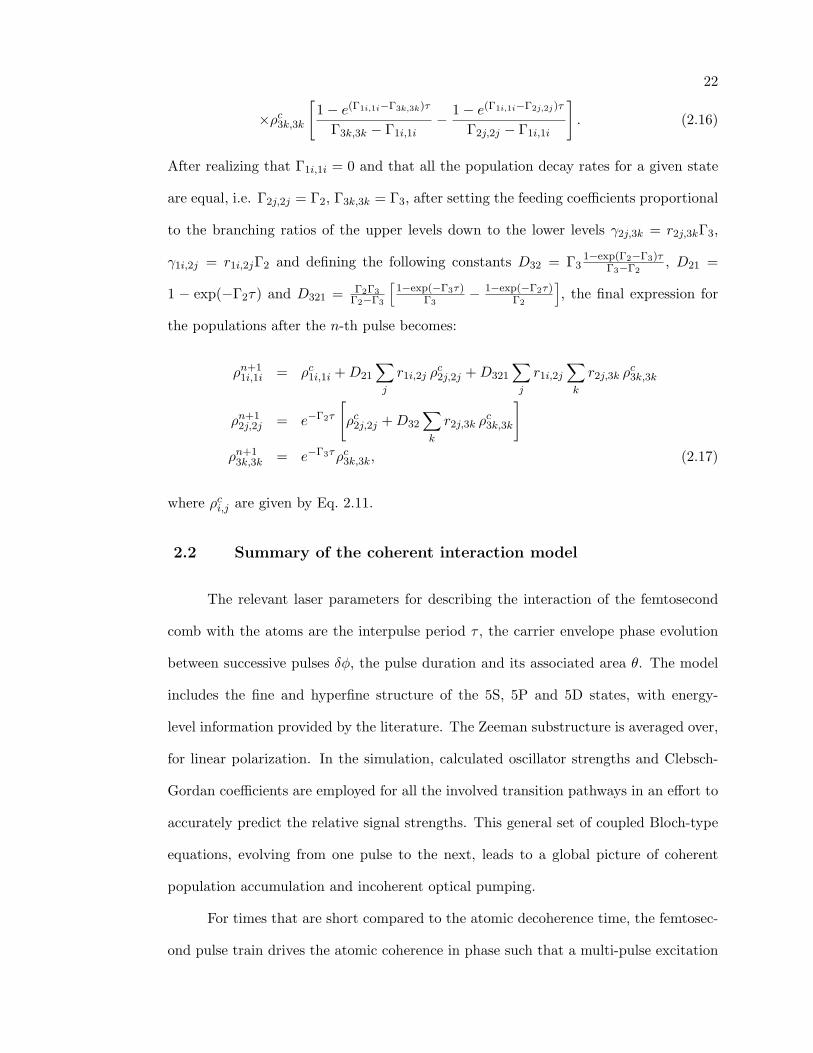
22
×ρc3k,3k
[1− e(Γ1i,1i−Γ3k,3k)τ
Γ3k,3k − Γ1i,1i− 1− e(Γ1i,1i−Γ2j,2j)τ
Γ2j,2j − Γ1i,1i
]. (2.16)
After realizing that Γ1i,1i = 0 and that all the population decay rates for a given state
are equal, i.e. Γ2j,2j = Γ2, Γ3k,3k = Γ3, after setting the feeding coefficients proportional
to the branching ratios of the upper levels down to the lower levels γ2j,3k = r2j,3kΓ3,
γ1i,2j = r1i,2jΓ2 and defining the following constants D32 = Γ31−exp(Γ2−Γ3)τ
Γ3−Γ2, D21 =
1 − exp(−Γ2τ) and D321 = Γ2Γ3Γ2−Γ3
[1−exp(−Γ3τ)
Γ3− 1−exp(−Γ2τ)
Γ2
], the final expression for
the populations after the n-th pulse becomes:
ρn+11i,1i = ρc
1i,1i + D21
∑j
r1i,2j ρc2j,2j + D321
∑j
r1i,2j
∑k
r2j,3k ρc3k,3k
ρn+12j,2j = e−Γ2τ
[ρc2j,2j + D32
∑k
r2j,3k ρc3k,3k
]ρn+13k,3k = e−Γ3τρc
3k,3k, (2.17)
where ρci,j are given by Eq. 2.11.
2.2 Summary of the coherent interaction model
The relevant laser parameters for describing the interaction of the femtosecond
comb with the atoms are the interpulse period τ , the carrier envelope phase evolution
between successive pulses δφ, the pulse duration and its associated area θ. The model
includes the fine and hyperfine structure of the 5S, 5P and 5D states, with energy-
level information provided by the literature. The Zeeman substructure is averaged over,
for linear polarization. In the simulation, calculated oscillator strengths and Clebsch-
Gordan coefficients are employed for all the involved transition pathways in an effort to
accurately predict the relative signal strengths. This general set of coupled Bloch-type
equations, evolving from one pulse to the next, leads to a global picture of coherent
population accumulation and incoherent optical pumping.
For times that are short compared to the atomic decoherence time, the femtosec-
ond pulse train drives the atomic coherence in phase such that a multi-pulse excitation
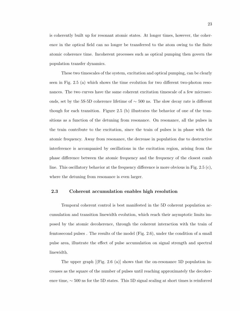
23
is coherently built up for resonant atomic states. At longer times, however, the coher-
ence in the optical field can no longer be transferred to the atom owing to the finite
atomic coherence time. Incoherent processes such as optical pumping then govern the
population transfer dynamics.
These two timescales of the system, excitation and optical pumping, can be clearly
seen in Fig. 2.5 (a) which shows the time evolution for two different two-photon reso-
nances. The two curves have the same coherent excitation timescale of a few microsec-
onds, set by the 5S-5D coherence lifetime of ∼ 500 ns. The slow decay rate is different
though for each transition. Figure 2.5 (b) illustrates the behavior of one of the tran-
sitions as a function of the detuning from resonance. On resonance, all the pulses in
the train contribute to the excitation, since the train of pulses is in phase with the
atomic frequency. Away from resonance, the decrease in population due to destructive
interference is accompanied by oscillations in the excitation region, arising from the
phase difference between the atomic frequency and the frequency of the closest comb
line. This oscillatory behavior at the frequency difference is more obvious in Fig. 2.5 (c),
where the detuning from resonance is even larger.
2.3 Coherent accumulation enables high resolution
Temporal coherent control is best manifested in the 5D coherent population ac-
cumulation and transition linewidth evolution, which reach their asymptotic limits im-
posed by the atomic decoherence, through the coherent interaction with the train of
femtosecond pulses . The results of the model (Fig. 2.6), under the condition of a small
pulse area, illustrate the effect of pulse accumulation on signal strength and spectral
linewidth.
The upper graph [(Fig. 2.6 (a)] shows that the on-resonance 5D population in-
creases as the square of the number of pulses until reaching approximately the decoher-
ence time, ∼ 500 ns for the 5D states. This 5D signal scaling at short times is reinforced

24
0.16
0.12
0.08
0.04
0.00
50 ρ 33
1086420Time (µs)
3.9 γ5D detuning
5S1/2 F=2 to 5D5/2 F=4 transition
0.4
0.3
0.2
0.1
0.0
10 ρ 33
20151050Time (µs)
on resonance 0.7 γ5D detuning 1.4 γ5D detuning
5S1/2 F=2 to 5D5/2 F=4 transition
0.4
0.3
0.2
0.1
0.0 1
0 ρ 33
302520151050Time (µs)
5S1/2 F=2 to 5D5/2 F=4 5S1/2 F=2 to 5D3/2 F=1
excitation
decay
(a)
(b)
(c)
Figure 2.5: Several aspects of population dynamics at short and long timescales:(a) Time evolution for two resonances, showing the short coherent excitation, followed bythe slow incoherent decay. (b) Temporal evolution for one of the previous transitions, fordifferent detunings from the atomic resonance, illustrating the destructive interferencethat results in the out-of-resonance condition. (c) Oscillation resulting from the phasedifference between the atomic frequency and the train of pulses.
25
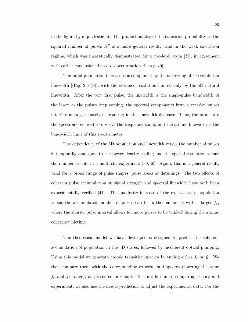
in the figure by a quadratic fit. The proportionality of the transition probability to the
squared number of pulses N2 is a more general result, valid in the weak excitation
regime, which was theoretically demonstrated for a two-level atom [39], in agreement
with earlier conclusions based on perturbation theory [40].
The rapid population increase is accompanied by the narrowing of the resolution
linewidth [(Fig. 2.6 (b)], with the obtained resolution limited only by the 5D natural
linewidth. After the very first pulse, the linewidth is the single-pulse bandwidth of
the laser; as the pulses keep coming, the spectral components from successive pulses
interfere among themselves, resulting in the linewidth decrease. Thus, the atoms are
the spectrometer used to observe the frequency comb, and the atomic linewidth is the
bandwidth limit of this spectrometer.
The dependence of the 5D population and linewidth versus the number of pulses
is temporally analogous to the power density scaling and the spatial resolution versus
the number of slits in a multi-slit experiment [39, 40]. Again, this is a general result,
valid for a broad range of pulse shapes, pulse areas or detunings. The two effects of
coherent pulse accumulation on signal strength and spectral linewidth have both been
experimentally verified [41]. The quadratic increase of the excited state population
versus the accumulated number of pulses can be further enhanced with a larger fr,
where the shorter pulse interval allows for more pulses to be ‘added’ during the atomic
coherence lifetime.
The theoretical model we have developed is designed to predict the coherent
accumulation of population in the 5D states, followed by incoherent optical pumping.
Using this model we generate atomic transition spectra by tuning either fr or f0. We
then compare them with the corresponding experimental spectra (covering the same
fr and f0 range), as presented in Chapter 5. In addition to comparing theory and
experiment, we also use the model prediction to adjust the experimental data. For the

26
case of the indirect 5P frequency measurements via the 5S-5D two-photon transitions,
described in Chapter 6, we use the theoretical prediction to modify the raw data (after
the adjustment, the data fall on top of a Lorentzian).
-2 -1 0 1 20.00
0.03
0.06
0.09
0.12
0.15Total Pulses:
10 20 50 80 100
D-S
tate
Pop
ulat
ion
Frequency (MHz)
(b)
(a)
0 20 40 60 80 100
1E-4
1E-3
0.01
0.1
Number of Pulses
D-S
tate
Pop
ulat
ion
Natural Linewidth (660 kHz)Quadratic Fit
0.1
1
10
100
Linewidth (M
Hz)
linewidth
D-population
Figure 2.6: (a) Left (right) axis shows calculated 5D population (linewidth) on resonancefor the closed two-photon transition versus total number of accumulated pulses. Thetime between pulses is ∼ 10 ns, and the system reaches its asymptotic values of signalamplitude and linewidth after ∼ 480 ns. The quadratic fit to the 5D population atshort times shows that the signal scales as the square of the number of pulses untilatomic decoherence limits the coherent pulse accumulation. (b) The corresponding 5Dresonance lineshape versus the number of pulses. During the first 10 pulses, the combstructure is not sufficiently developed to offer appreciable signal or resolution.

Chapter 3
Experimental Apparatus: the femtosecond Ti:S setup and the MOT
This chapter discusses the two primary components of the experimental setup,
the femtosecond laser and the MOT. I will first present the idea for the Ti:S laser
stabilization and then describe one of the most commonly used self-referencing schemes.
I will conclude by briefly discussing the stabilization of the cw lasers and the setup used
for cooling and trapping in the MOT. Chapter 4 will present the integration of the
femtosecond laser and the MOT.
3.1 The femtosecond Ti:S laser and its stabilization setup
Recent advances in controlling the pulse repetition period and the carrier-envelope
phase of mode-locked lasers have ushered in a series of novel applications using their
frequency combs [42]. In the introduction I presented some of the fundamental aspects
of mode-locked lasers. In this section, I will review some of the basic concepts be-
hind carrier-envelope phase stabilization and I will explain how the two dynamic laser
parameters are optically detected and stabilized in the experiment. Stabilization of
the two degrees of freedom is a necessary step for using these lasers for spectroscopic
applications.

28
3.1.1 Stabilizing the two degrees of freedom of mode-locked lasers
For the experiment, we used a home-built titanium-doped sapphire (Ti:S) laser
pumped by a 5 W single-frequency, diode-pumped, frequency-doubled Nd:YVO4 laser
(Coherent Verdi) operating at 532 nm. The Ti:S laser generates a 100-MHz pulse train
with pulse widths on the order of 15 fs and energies of about 5 nJ per pulse, using
Kerr lens mode-locking (KLM). A diagram of our KLM laser is shown in Fig. 3.1. The
configuration used is a standing-wave, folded geometry, with the cavity delimited by
two flat mirrors: the laser end mirror (EM) and the partially reflective output coupler
(OC). The nonlinear gain element for the laser cavity is the Ti:S crystal. The passive
mode-locking mechanism employed here is the nonlinear Kerr Effect, which gives an
increase in the index of refraction of the crystal as the optical intensity is increased (self-
phase modulation, self-focusing, see for example [43]). The Ti:S acts like a nonlinear
lens, slightly focusing the intracavity beam, but it also spreads the pulses temporally
through normal dispersion (the long wavelengths travel faster than the short ones). As
a consequence, a sequence of two prisms is used to compensate for the group velocity
dispersion (GVD) in the crystal: the first prism spatially disperses the pulse, leading the
long wavelengths to traverse more glass in the second prism than the short wavelengths.
The beam is still horizontally dispersed after the second prism, though collimated. Upon
reflection by the laser cavity EM, the pulse travels again through the pair of prisms,
thus canceling the spatial dispersion.
As mentioned before, fr determines the mode spacing and is inversely propor-
tional to the cavity length L, fr = vg
L , while f0 sets the absolute comb position and is
proportional to the intracavity dispersion, f0 = ωc2π (1 − vg
vp). They are both influenced
by the group velocity vg, but there is no apparent f0 dependence on the laser cavity
length. Ideally one would like to control the two parameters independently. One ad-
justable parameter can be the cavity length, for fr control; yet, an additional degree of

29
PUMP
EM
OC
FMCM1 CM2
P2P1
Ti:S crystal
δLβ
L
Figure 3.1: Optical layout of the KLM Ti:S laser used in the experiment; the end mirror(EM) and the output coupler (OC) are the two flat mirrors bounding the cavity, usedfor the f0 and fr stabilization, respectively. The two prisms P1 and P2 are used fordispersion compensation.
freedom is needed for changing vg. The one employed in my laser was first suggested
in 1999 by the Hansch group [44] and uses small-angle rotations about the vertical axis
of the laser EM. As previously stated, the different spectral components in the laser
beam are horizontally spread out at the EM, leading to a linear relationship between
the spatial coordinate and the wavelength. For small angle (β) changes, there is a linear
path length change, i.e. phase shift, with frequency. This is effectively a group delay,
linear with the angle. Under this assumption that the swivel mirror changes the group
delay by a small amount ∼ β, it can be shown [28] that f0 is only controlled by β, while
fr depends on both β and L. Therefore, one can use the swivel angle β to control f0 (this
will also change fr!), and the cavity length L to compensate for the subsequent change
in fr. Details of the experimental implementation of the vg, and hence f0, control will
be given in 3.1.5.
3.1.2 Stabilization of the laser repetition rate
The laser repetition frequency fr is a radio frequency (rf) ∼ 100 MHz and is
measured directly using a fast photodiode. To reduce the increase in phase noise that
is due to the large frequency multiplication factor up into the optical region (∼ 106), a

30
higher harmonic of the pulse repetition rate is used for stabilization. A portion of the
pulse train is detected with a high-speed photodetector; the 10th harmonic of fr at 1
GHz is filtered and amplified (to 0 dBm, suitable for the rf port of a double-balanced
mixer) and then phase-locked to the 1 GHz provided by a stable microwave source.
The error signal obtained by comparing against this reference frequency is integrated,
filtered and amplified in a JILA-built loop filter (LF) and then used for active feedback
to the laser, as shown in Fig. 3.2. Cavity length corrections are controlled with a small
(∼ 5 mm) tube piezoelectric transducer (PZT), on which the output coupler of the laser
has been mounted. All the comb modes are moved together by this translating PZT
which varies the laser cavity length.
DDS
JILA LF
HV driver (1 kV)
1 GHz Wenzel
rf amplifier
N fr
1GHz BPF
Ti:S Laser
frequency counter
to Output Coupler (translating PZT)
to f0 stabilizationand MOT
Figure 3.2: Stabilization diagram used for phase-locking of the laser repetition rate fr;BPF stands for band-pass filter, DDS for direct digital synthesizer and LF for loop filter.More details are given in the text.
Several stable rf oscillators were tried as references for the repetition rate (I will
address this issue further in Chapter 4) and in the end a custom-made Wenzel oscilla-
tor, based on a crystal oscillator that has a very good short-term frequency stability,
was settled upon. The short-term stability of the rf source is very important, given
the huge multiplication factor up into the optical domain. Unfortunately, the Wenzel
tuning range is only 3.2 kHz around 1 GHz, corresponding to a 320 Hz tunability of
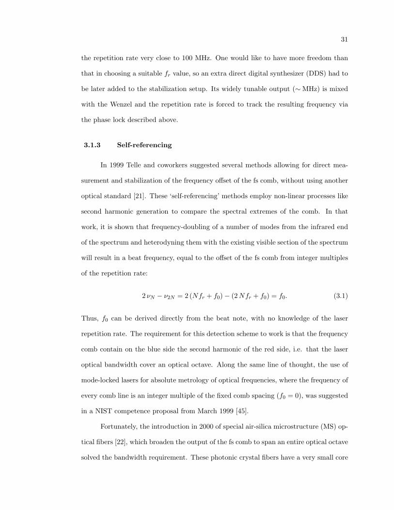
31
the repetition rate very close to 100 MHz. One would like to have more freedom than
that in choosing a suitable fr value, so an extra direct digital synthesizer (DDS) had to
be later added to the stabilization setup. Its widely tunable output (∼MHz) is mixed
with the Wenzel and the repetition rate is forced to track the resulting frequency via
the phase lock described above.
3.1.3 Self-referencing
In 1999 Telle and coworkers suggested several methods allowing for direct mea-
surement and stabilization of the frequency offset of the fs comb, without using another
optical standard [21]. These ‘self-referencing’ methods employ non-linear processes like
second harmonic generation to compare the spectral extremes of the comb. In that
work, it is shown that frequency-doubling of a number of modes from the infrared end
of the spectrum and heterodyning them with the existing visible section of the spectrum
will result in a beat frequency, equal to the offset of the fs comb from integer multiples
of the repetition rate:
2 νN − ν2N = 2 (Nfr + f0)− (2 Nfr + f0) = f0. (3.1)
Thus, f0 can be derived directly from the beat note, with no knowledge of the laser
repetition rate. The requirement for this detection scheme to work is that the frequency
comb contain on the blue side the second harmonic of the red side, i.e. that the laser
optical bandwidth cover an optical octave. Along the same line of thought, the use of
mode-locked lasers for absolute metrology of optical frequencies, where the frequency of
every comb line is an integer multiple of the fixed comb spacing (f0 = 0), was suggested
in a NIST competence proposal from March 1999 [45].
Fortunately, the introduction in 2000 of special air-silica microstructure (MS) op-
tical fibers [22], which broaden the output of the fs comb to span an entire optical octave
solved the bandwidth requirement. These photonic crystal fibers have a very small core

32
diameter (1.7 µm), providing a very tight spatial confinement that generates very high
intensities (∼TW/cm2). They have been engineered to exhibit zero GVD near 800 nm,
which minimizes the temporal spread of the pulses propagating in the fiber over signif-
icant distances (several cm). The main non-linear effect leading to spectral broadening
in the fiber is strong four-wave-mixing among the different frequency components in the
input pulse spectrum, which generates new spectral components, while maintaining the
periodicity of the incoming frequency comb. The spectral bandwidth at the output of
the MS fiber can extend well beyond one optical octave e.g. 400 to 1200 nm.
The first experimental implementation of the self-referencing technique using ex-
ternal broadening in a MS fiber, followed by doubling of the 1040 nm light and mixing
with the fundamental at 520 nm, was reported by Jones and co-workers in 2000 [1].
Ultra-broadband mode-locked lasers whose direct output spans on optical octave, al-
lowing for direct self-referencing and stabilization of the pulse train, have also been
recently demonstrated [7].
3.1.4 The ν-to-2 ν prism interferometer
To achieve spectral broadening, ∼ 120 mW of the fs laser output light (∼ 500
mW) are coupled into a ∼ 7-cm piece of MS fiber. The output of the fiber is then sent
into an ν-to-2 ν interferometer for self-comparison.
The configuration chosen for the interferometer is the so-called ‘prism-pair’ geom-
etry, presented in Fig. 3.3. The sequence of SF10 prisms (8-cm prism separation) spa-
tially separates the green (e.g. 532 nm) and red (e.g. 1064 nm) components of the
spectrum, which are then reflected by two mirrors located very close to each other. The
green-reflecting mirror is mounted on a translation stage, to easily adjust the temporal
overlap between the red and green pulses at the detector. When the interferometer is
well aligned and working, the distance between the end mirrors is ∼ 1 mm.
The beams retrace their path through the prism pair with a slight vertical offset

33
Ti:S Laser
fr lock
ν- to-2ν interferometer
MS fiber
to MOT60 X 60 X
532 nm filter
BBO
polarizer
photodetectorf0
(bandwidth 10 nm)
Figure 3.3: Diagram of the prism interferometer used for the detection of the comboffset frequency. The broad spectrum from the MS fiber is sent into a prism pair forspatial dispersion. The light near 532 nm is reflected by one end mirror, while thelight near 1064 nm hits a second end mirror. Both beams are reflected back throughthe prism pair, recombined and then sent through a nonlinear BBO crystal tuned forefficient second harmonic generation at 1064 nm. The output is filtered, and the f0 beatis detected on a PD.
in order to be picked off by a mirror positioned below the incoming beam. The pick-
off mirror sends the recombined beams to a lens, which focuses them into a nonlinear
crystal (1-mm BBO, type I phase-matching), angle-tuned for efficient second harmonic
generation at 1064 nm.
Two types of green light are present at the output of the BBO crystal: the
frequency-doubled beam obtained from the infrared part of the spectrum and the fun-
damental green coming out of the MS fiber; the polarization of the frequency-doubled
green is rotated by 90 degrees with respect to the fundamental green. A 10-nm interfer-
ence filter centered at 532 nm removes the extra, non-contributing spectral components,
while a polarizer ensures that the polarizations of the two green beams are aligned along
the same axis. Spatial overlap and mode-matching of the two beams are essential for a
good signal-to-noise ratio (S/N) of the beat signal. A photodiode detects their difference
frequency, the f0 beat, along with the laser repetition rate. In reality, the detected beat

34
arises from mixing of thousands of comb lines, not just the two frequencies mentioned,
giving a better S/N. In the experiment, the typical S/N of the offset beat is ∼ 45 dB in
a 100 kHz resolution bandwidth.
The prism pair geometry is advantageous to use compared to other configurations,
e.g. a Mach-Zender interferometer, because most of its elements are common-mode (the
only differential path is the prism pair region), which makes it easier to align and tweak.
3.1.5 Stabilization of the laser offset frequency
The output of the ν-to-2 ν PD is sent through two 50 MHz low-pass filters (LPF),
to reduce all the unnecessary rf frequencies in the spectrum (otherwise, they would
saturate the subsequent amplifiers), then a small portion of the signal is sent via a
directional coupler to an rf spectrum analyzer for monitoring of the beat note. The
main signal is amplified to ∼ -5 dBm and then frequency-prescaled (divided by 64)
before its phase is compared to a stable rf oscillator such as a DDS. Unlike the fr lock
which employs an analog phase detector, the stabilization circuit used for f0 employs a
digital phase detector (DPD), which provides both a frequency and a phase lock. This
allows for a larger capture and locking range than the double-balanced mixer case and
increases the stability of the lock. Again, the error signal derived by comparing against
the reference frequency is integrated, filtered and amplified in a JILA LF (see Fig. 3.4)
and then sent to the laser for frequency correction. Note that the local oscillators used
for the fr and f0 stabilization are all referenced to the same local commercial cesium
clock.
As announced earlier in section 3.1.1, f0 control is carried out by fine-tuning the
laser end mirror angle using a twister PZT. The twister PZT used to tilt the end mirror
is a 0.5 inch diameter cylinder, about 0.5 inch long, that has been modified such that the
outer electrical surface is split to allow for the two outer sides to have different voltages
with respect to the inner surface of the PZT. When applying opposite-sign voltages to

35
Ti:S Laser
fr lock
to MOT
rf amplifier
f0
50 MHz LPF
spectrum analyzer
HV driver (±150 V)to End Mirror (tilting PZT)
DDS
DPD
ν-to-2νinterferometer
JILA LF
Figure 3.4: Stabilization diagram used for phase-locking of the laser offset frequency f0;LPF stands for low-pass filter, DPD for direct phase detector, DDS for direct digitalsynthesizer and LF for loop filter. The details are given in the text.
the two sides, one contracts, while the other expands, with the net effect of an angle
change for the end mirror mounted on the PZT. As mentioned before, this is effectively
a group delay, which depends on the voltage sent to the PZT. Changing the voltage in
the 0 to ±150 V range allows for scanning of the offset frequency beat over its full range
of ∼ 50 MHz.
Another method of adjusting and stabilizing f0 is employing an acousto-optic
modulator (AOM) to control the pump laser power. Modulating the pump laser power
actually affects several laser parameters. Systematic studies of intensity-related dynam-
ics in mode-locked Ti:S lasers have been recently undertaken [46,47] to understand the
effects on fr and f0.
To summarize, fr and f0 stabilization and referencing to an atomic clock result
in knowledge of the absolute frequencies of the ∼ 106 comb lines, with an accuracy only
limited by the frequency reference used. The stabilized comb can now be employed as a
precision frequency ruler for any optical frequency in the visible to near-infrared range.

36
3.2 The MOT
The magneto-optical trap (MOT) is currently the starting point for many ex-
periments with laser-cooled atoms. Cold atoms are used for precision measurements,
atom interferometers, atomic clocks, to name just a few examples. Advances in laser
cooling of alkali atoms [48] have also paved the way to producing the first Bose-Einstein
condensates and degenerate Fermi gases [49–51]. In particular, vapor-cell traps [52] like
the one used in this experiment, are simple and versatile tools for many experiments
with cold atoms.
Our experiment was performed on a sample of laser-trapped and -cooled Rubid-
ium 87 atoms (see Fig. 4.2 for a detailed 87Rb level diagram, I=3/2). The 5S1/2 → 5P3/2
cooling transitions can be easily accessed with commercially available laser diodes cen-
tered at 780 nm, making 87Rb a convenient choice for laser cooling and trapping. We
use two lasers to trap and cool the atoms. The cooling beams are ∼10 MHz red-detuned
from the 5S1/2 (F=2) → 5P3/2 (F′=3) cycling transition. An additional laser, the so-
called ‘repumper’, tuned to the 5S1/2 (F=1) → 5P3/2 (F′=2) transition, is needed to
return the atoms to the cooling cycle whenever they decay to the F=1 ground level,
thus preventing them from falling dark due to optical pumping.
3.2.1 Diode lasers: description and stabilization
The laser diodes used are Sharp LT024MD (specified output power of 20 mW)
for the repump laser (RL) and Sanyo DL7140-201 (specified output power of 70 mW)
for the trap laser (TL). They are configured in an external cavity geometry, based on a
design described in reference [53,54], with ∼ 3.5 cm extended cavity length. The lasers
employ a diffraction grating (1200 lines/mm) aligned in the Littrow configuration [55]
to couple the first diffraction order back into the laser. One PZT controls the horizontal
tilt of the grating, permitting adjustments of the laser wavelength. A change in the PZT

37
length alters the grating angle and the external cavity length at the same time, allowing
for continuous scans of typically ∼ 5 GHz. Additionally, the grating is mounted on a
fast disk PZT, which is servoed together with the laser diode current to stabilize the
laser frequency.
Both diode lasers are locked to the specified atomic transitions using standard
saturated absorption spectroscopy [53], which yields sub-Doppler hyperfine lines that
are used to frequency-stabilize the laser (see Fig. 3.5). The TL is locked to the red side
of the saturated absorption peak; a side lock is not ideal, since the locking set point
is inevitably dependent on power broadening of the transition lines. We use acousto-
optic modulators (AOMs) to create beams at various detunings and also to control the
timing of the lasers in the experiment. The TL light is steered through two AOMs: the
first AOM deflects a small amount of power (-1 order) into the saturated absorption
spectrometer, for frequency stabilization. The second AOM acts as a shutter for the
light, by directing the negative first order diffracted beam to the MOT cell. Thus, the
MOT red detuning is set by the side lock along with the frequency difference of the two
AOMs.
The RL is locked to the peak of the crossover transition between the 5S1/2 (F=1)→
5P3/2 (F′=1) and the 5S1/2 (F=1)→ 5P3/2 (F′=2) transitions, using modulation side-
bands at 4.6 MHz, written directly on the diode-laser current (the laser output current
can be modulated rapidly by sending a voltage into the rf modulation input, this in turn
will modulate the frequency of the laser). The signal from the RL saturated absorp-
tion spectrometer is detected with a homemade resonant photodetector (PD) and then
compared in a double-balanced mixer with the local oscillator at 4.6 MHz, resulting
in dispersion curves for all the features in the saturated absorption spectrum [56, 57].
The value of these dispersion curves changes sign at the peak, allowing for a lock at the
zero-crossing of the error signal. Since the RL is offset peak-locked, an AOM is needed
to shift the frequency into resonance with either the 5S1/2 (F=1)→ 5P3/2 (F′=1) or the

38
85Rb F=3 to F'=
432
85Rb F=2 to F'=
32
1
RLlock
TLlock
87Rb F=1 to F'=
21
0
87Rb F=2 to F'=
3 21
2 / 3
1 / 31 / 2
700 MHz
Figure 3.5: Saturated absorption spectra, showing the hyperfine structure of the5S1/2 → 5P3/2 transitions for the two Rb isotopes. The numbers labeling the hyperfinepeaks correspond to F′ states in the 5P3/2 manifold. Note that the spectra contain bothtrue Doppler-free resonances (numbered peaks) and crossover resonances. The crossoverresonances occur at frequencies (νa +νb)/2 for each pair of true resonances at frequencyνa and νb, as exemplified for the bottom spectrum.

39
5S1/2 (F=1)→ 5P3/2 (F′=2) transition. We opted for the latter and thus the positive
first order deflected beam is sent to the MOT vapor cell. In order to operate the trap
at zero repump detuning, the driving frequency for the RL AOM is equal to exactly
half of the F′=1– F′=2 5P3/2 hyperfine interval (78.45 MHz). This AOM is a fast and
convenient switch used to turn off the RL beam whenever needed.
3.2.2 MOT details
The main TL beam is spatially filtered by a 70 µm pinhole, which reduces the
high-frequency spatial modes, and collimated to roughly a 1-cm beam diameter with
a beam-enlarging telescope. It is then divided into three separate, intensity-balanced
beams using λ/2 plates and polarizing beamsplitter cubes. The three beams are sent
to the experiment glass cell using 1-inch diameter optics, in a standard retro-reflected
MOT configuration [58]. The atoms are caught in the MOT using these three pairs of
orthogonal, circularly-polarized beams in the typical σ+−σ− arrangement, and detuned
∼ 10 MHz to the red of the atomic resonance. The RL beam is directed into the cell
along one of the TL beams. We monitor the beams in the cell and the position of the
trapped cloud with a low-cost CCD camera.
We load the MOT from the vapor produced by Rb dispensers (‘getters’) in a
cylindrical glass cell. The vapor cell is continuously pumped by an ion pump and
typically reaches a background pressure of 10−9 Torr. The source of Rb consists of
three nichrome (Ni-Cr alloy) dispenser strips, connected in parallel and placed in a
small side arm of the cell. They contain a Rb salt and release atoms through a chemical
reaction when an electric current is passed through them and heats the nichrome. Only
one dispenser is used at a time, and the operating current is usually 3.5 A.
The quadrupole magnetic field necessary to operate a MOT is provided by a pair
of anti-Helmholtz coils. The two coils are wound from ‘magnet wire’, i.e. Cu wire (∼ 1
mm diameter) coated with an insulating material, and are wrapped around the axis of

40
the cylindrical cell. Each coil is 7 cm in diameter and has 33 turns. The coils are spaced
5.5 cm apart and are supplied with ∼ 4.5 A, generating a magnetic field gradient of ∼
10 G/cm.
Stray magnetic fields, due mainly to the Earth’s field, can shift the zero-point of
the MOT field. They are compensated by three pairs of orthogonal Helmholtz coils.
The glass cell is surrounded by these pairs of shim coils, each run by a different current
supply. In the early stages of the experiment, the beam alignment and ambient magnetic
field compensation were verified by monitoring the isotropy of the molasses expansion.
We were aiming for a slow and uniform expansion of the atomic cloud upon switching off
the quadrupole field. At a later stage, after obtaining the two-photon signal as described
in Chapter 4, we realized that we could use it to find the zero-point of the magnetic
field.
Resonance fluorescence from the atoms is detected with a photodiode (PD), lead-
ing to an estimate of the atom number based on the PD current, the PD responsitivity,
the solid angle of the light collected by the imaging lens, the energy of a photon and
the optical scattering rate. We typically trap 5×10⁶ atoms in a 0.5 mm diameter MOT
with a 1/e lifetime between 3 and 5 s.
After collecting the atoms in the MOT, we transfer them to optical molasses [59]
for further cooling using polarization gradients (PGC). To experimentally implement
PGC, the quadrupole field gradient is turned off, the TL is further red-detuned from
resonance (∼ 40 MHz) and the TL beam intensity is decreased. The resulting sub-
Doppler cloud temperature established by PGC is ∼ 15 µK, providing an ideal initial
condition for spectroscopy.
I have presented here the basic operation details of the MOT. In Chapter 4 I will
describe how the trapped atoms are probed with the frequency comb of a femtosecond
laser.
Chapter 4
Characterization of the systematic effects related to direct frequency
comb spectroscopy
We would like to use a phase-stabilized femtosecond laser comb directly for high-
resolution spectroscopy and absolute optical frequency measurements of one- and two-
photon transitions in laser-cooled 87Rb atoms. We defer further discussion of the spec-
troscopy, however, until we have explored some of the important sources of possible
systematic error [60]. In section 4.4.2, I will discuss both experimentally and theoret-
ically the mechanical action of the probe on the atoms. I will then present the AC
Stark frequency shifts induced by the femtosecond light in section 4.4.3. Finally, the
last systematic error we studied, arising from Zeeman shifts, will be presented in sec-
tion 4.4.4. As briefly mentioned in Chapter 3, the short-term stability of the reference
used to stabilize the repetition rate also warrants attention. We will see that the main
contributions to the systematics are those arising from mechanical effects and the AC
Stark shifts.
4.1 Doppler-free two-photon transitions with cw and pulsed sources
Study of two-photon transitions to achieve high-resolution spectroscopy or to
maximize the excitation efficiency of a desired state has been an active field of research
in the past decades. Doppler-free multi-photon transitions have been theoretically stud-
ied by Cagnac et al. [61]. The first experimental demonstrations followed shortly, by

42
observing two-photon absorption resonances in Na using tunable dye lasers [62–64]. The
effects of Doppler broadening in the vapor were eliminated by making the atoms absorb
one photon from each of the two equal-energy, counterpropagating cw beams (Fig. 4.1,
top panel).
In a closely related experiment, optical beams were arranged to both (i) propagate
in opposite directions as well as (ii) have unequal frequencies (Fig. 4.1, bottom panel).
This configuration was used to demonstrate resonantly enhanced two-photon absorption
in Na vapor [65]. The two-photon absorption cross-section was enhanced by over 7 orders
of magnitude, by letting one of the photons be nearly resonant with an intermediate
state. Doppler effects were greatly reduced by using counter-propagating beams, but
not totally eliminated. In a different experiment, the two-photon transition rate was
resonantly enhanced by using a fast atomic beam [66], where the high atomic velocities
allowed for Doppler tuning of an intermediate state into exact resonance in the rest
frame of the atom.
DL Equal Frequency
cell
5D
5P
5S
DL1 DL2Two Color
cell
=> 107 enhancement
5D
5P
5S
Figure 4.1: Schematic of Doppler-free two-photon spectroscopy in a cell, with equal-frequency (top) and two-color (bottom) counterpropagating beams.

43
Doppler-free two-photon spectroscopy has also enabled the observation of opti-
cal Ramsey fringes. In the experiments of Salour [40, 67] the atoms have interacted
with two time-delayed phase-coherent laser pulses, while Baklanov et al. have suggested
two spatially separated light standing waves [68]. Note that Bergquist et al. have ob-
served Ramsey fringes in the saturated-absorption signal from a fast beam of Ne* atoms
crossing three and four equally spaced spatially separated standing-wave beams [69].
With regard to employing pulsed sources, high-resolution two-photon spectroscopy
using picosecond pulsed light and hence, without any appreciable intermediate-state in-
teraction or absolute frequency reference, has been previously demonstrated [27], with a
recent extension to laser-cooled samples [70]. Cold atoms confined in a MOT provide an
almost-Doppler-free environment for use in spectroscopic studies. For the case of two-
photon transitions, where the absorption cross sections are relatively small and thus the
required intensities are rather large, the cold sample mitigates the Doppler broadening
arising from the strong focusing needed.
The advent of ultrafast lasers combined with pulse-shaping techniques has led to
new schemes [14, 71], where two-photon transitions which constitute the lowest-order
nonlinear interaction, are used as a benchmark system. In particular, Silberberg and
coworkers have shown that the two-photon absorption rate is maximized for transform-
limited pulses only in the case of transitions without any resonant intermediate state.
For transitions involving a nearly resonant intermediate state, an enhancement by a
factor of 7 of the two-photon absorption rate in Rb vapor has been obtained by shaping
the pulse [71]. Thus, the final population transfer was controlled by manipulating the
coherence properties of the optical field.
4.2 Background for the technique of two-photon DFCS
We directly interrogate a sample of laser-cooled 87Rb atoms with a frequency
comb and induce two-photon transitions. This capability is enabled by the bandwidth

44
741 nm
639.4 MHz7S1/2 F’’=2
F’’=1
22.9 MHz
28.8 MHz
15.9 MHz5D5/2F’’=1F’’=2
F’’=3F’’=4
27.9 MHz13.5 MHz
44.2 MHz5D3/2F’’=3F’’=2
F’’=1F’’=0
156.9 MHz72.2 MHz
266.6 MHz5P3/2F’=3F’=2
F’=1F’=0
816.6 MHz5P1/2 F’=2
F’=1
6834.6 MHz5S1/2 F=2
F=1
795 nm
780 nm
776 nm
762 nm
7 122 413 MHz
88 857 MHz
18 224 929 MHz
377 104 390 MHz
386 252 075 MHz
Figure 4.2: Schematic of the 87Rb energy levels participating in the one- and two-photon transitions we studied, including the wavelength and energy level information.The levels highlighted in red correspond to the closed 2-3-4 transition pathway (section4.4). We have investigated seven two-photon transitions, as detailed in section 5.2.

45
associated with the femtosecond pulse, which is sufficiently broad that many fine and
hyperfine atomic states (see Fig. 4.2) can be excited by tuning the relevant comb com-
ponents into resonance. The two independent parameters fr and f0 provide freedom in
choosing an appropriate frequency comb for control of resonant signal enhancement via
the intermediate 5P1/2 and 5P3/2 states.
Our experimental prototype system to study DFCS is therefore a set of two-
photon transitions from the ground-state 5S1/2 to the excited 5D3/2 and 5D5/2 states,
enhanced by the 5P intermediate states as shown in Fig. 4.3. The dipole-allowed inter-
mediate states, 5P3/2 and 5P1/2, are located ∼ 2 and 17 nm (i.e. ∼ 1 and 8 THz) below
the energy degenerate virtual level for the two-photon transition, respectively (Fig. 4.2).
The lifetime of the 5P intermediate states is 27 ns, the lifetime of the 5D states is 241
ns and the lifetime of the 7S states is 88 ns [72].
5P
5D
δSP
δSD
5S
νSP = N fr + fo
phase-coherentcomb
fr
…
f0
νPD = M fr + fo
Figure 4.3: Resonantly enhanced two-photon transition with detunings δSP and δSD
for the pair of comb modes that makes the dominant contribution to the transitionprobability.
As mentioned in Chapter 1, the optical frequency of a particular comb mode

46
can be expressed as νN = Nfr + f0, where fr is the pulse repetition rate, f0 is the
carrier envelope offset frequency, and N is an integer on the order of 106. The sum
frequency of the light from two comb lines labeled by N and M is given by ν2γ =
(N + M)fr + 2f0. There are several hundred thousand comb pairs (N , M) that yield
the same sum frequency and thus could contribute to the transition amplitude when ν2γ
is resonant with the two-photon transition (δSD ∼ 0 as shown in Fig. 4.3). However, in
estimating their relative contributions, it is necessary to consider the intermediate 5P
states that provide resonant enhancement.
When one of the comb lines is tuned near resonance with one of the 5S-5P transi-
tions (δSP ∼ 0 as shown in Fig. 4.3), the resonant enhancement causes the corresponding
pair to make the dominant contribution to the two-photon transition over all of the other
pairs. This dominant contribution is reinforced by destructive quantum interference be-
tween comb pairs symmetrically detuned on either side of the P state, resulting in a
∼ 180◦ phase difference [71]. For the non-resonant configuration of comb modes de-
tuned ±kfr/2 (k ≥ 1, odd integer) away from the P state, with all pairs satisfying the
two-photon resonance, the transition amplitudes associated with (+k) and (-k) modes
will again destructively interfere. However, there will be a net non-resonant contribu-
tion due mainly to the existence of multiple P states that break the symmetry of the
comb distribution. This destructive interference can be made constructive by flipping
the spectral phase about the P state [71].
The two-photon transition spectrum is obtained by scanning fr or f0; their pre-
cisely measured values, along with (N , M), determine all relevant atomic energy levels
in absolute terms.
4.3 Experimental method
The experiment is performed with an optical frequency comb (emitted from a
20-fs, 100-MHz repetition rate, mode-locked Ti:sapphire laser) centered at 778 nm with

47
onTwo-photontiming diagram
500 µs
fs light
MOT7.5 ms
PGC2 ms
t
Normalized Light Intensity1.00.80.60.40.20.0
16012080400
τ
Time,τ (µs)
Shutter is on at τ=6 µs
Figure 4.4: Timing scheme for the 100 Hz experiment cycle. The atoms are first loadedin the MOT for 7.5 ms and then, at the end of the loading time, the trapping quadrupolemagnetic field is extinguished (not shown). Additional cooling of the atoms is done withpolarization gradients (PGC) for 2 ms. All MOT-related fields are turned off at the endof the PGC stage. At this point, the femtosecond laser is switched on using the liquidcrystal shutter (30-µs response time). The 500-µs zoom window shows the variableprobe window (τ) used for the two-photon measurements. Signals are averaged overhundreds of 10 ms experiment cycles.

48
PMT
Computer Photon CounterTiming
MOTShutterFs
Beam
Figure 4.5: Shown here is the optical configuration for the counterpropagating beams,implemented in all our two-photon studies, including those described in Chapters 5 and6. The 420-nm blue fluorescence detected by the PMT is sent to a photon counter andthen read into the computer.
a full width at half maximum bandwidth of ∼ 55 nm (∼ 26 THz). There is ∼ 200 nW
of power in each of the comb lines resonant with the 5S-5P and 5P-5D transitions. The
light is typically focused to a beam waist of 130 µm, giving an on-axis intensity of ∼ 0.8
mW/cm2 in each comb line. For time-resolved studies, the sample is exposed to light
by a liquid crystal with a 30-µs response time.
As described in Chapter 3, the atomic source is a cloud of 87Rb trapped and
cooled in a vapor-cell MOT. As shown in Fig. 4.4, the typical loading cycle used for the
MOT is 100 Hz and the sequence of the experiment is as follows: the atoms are loaded
in the MOT for 7.5 ms, then the quadrupole magnetic field for the trap is switched off,
the atoms are further cooled with polarization gradients (PGC) for 2 ms, then all the
MOT beams are extinguished, the femtosecond comb beam is switched on for 500 µs
using the shutter, and finally, the 420 nm fluorescence is detected.
The cw MOT repumping laser controls the initial populations of the two ground-
state hyperfine levels. During the actual probing period, the femtosecond comb itself
acts as a repumper, allowing one to maintain a stable population in the initial ground
state.

49
The excited 5D state population is determined from the 5D-6P-5S radiative cas-
cade: the atoms relax to the 6P state and then decay down to the ground state, emit-
ting photons at 420 nm. These blue photons are detected with a photomultiplier tube
(PMT) centered (Fig. 4.5) at 420 nm and are counted and subsequently time-binned
with a multi-channel photon counter, with a typical integration time of 10 µs. In general,
signals are averaged over hundreds of 10-ms experiment cycles.
One of the main problems in acquiring reproducible data is that the femtosecond
laser is located on one optical table, and the Rb apparatus on a different optical table
∼10 meters away. This creates serious beam-pointing instabilities. We have imple-
mented a beam-steering servo based on a quadrant photodiode and a tip/tilt mirror to
actively control the beam pointing.
4.4 Main systematic effects
As in the case of precision spectroscopy performed with cw lasers, the use of the
femtosecond comb as a precision probe requires a careful understanding of all systematic
effects. Indeed the dominant effects are the mechanical effect of the optical comb on the
atomic motion, the light shift by the probe laser, and the Zeeman frequency shifts. The
short-term stability of the rf source used to reference fr is also important, as discussed
in the next section.
We have performed all studies of the systematics involved on one sample transi-
tion, namely the 5S1/2 (F=2)→ 5P3/2 (F′=3)→ 5D5/2 (F′′=4) closed two-photon tran-
sition, which gives the best signal-to-noise ratio. A closed transition is defined to be a
transition which decays back to the hyperfine level from which it was excited. I have
highlighted in Fig. 4.2, in red, the states involved in the only closed two-photon transi-
tion occurring in 87Rb among the levels shown. This closed transition occurs when the
atoms start in the F=2 state, are then excited to the F′=3 state, and then to the F′′=4
state and finally decay back to the F=2 state (through either the 5P or the 6P channel).

50
f0 tuning of fs laser
f0
to MOT
OC
EM
β
f0 tuning and locking electronics
5P
5D
5S
PMT
6P
2500
2000
1500
1000
500
0
222120191817
f0 (MHz)
Sign
al (a
.u.)
Typical 2-3-4two-photonlineshape
Figure 4.6: The top panel shows the experimental setup for scanning f0 and the lowerpanel presents a typical 5S1/2 (F=2)→ 5P3/2 (F′=3)→ 5D5/2 (F′′=4) (‘2-3-4’) closedtwo-photon lineshape obtained from such a frequency scan. The decay channel used fordetecting the population of the 5D excited state is also shown.

51
In contrast, note for example that the transitions F=2 to F′=1 or 2 are not closed, since
they have a decay channel to the F=1 ground hyperfine level and thus, the atoms do
not all return to the initial F=2 state. In summary, the 2-3-4 is a closed transition
because for each of the two steps 5S-5P and 5P-5D, the electric dipole selection rule
(∆F = 0,±1) prevents the excited atoms from falling into the F=1 ground state.
As a convention, any two-photon process starting in F=2 that accesses the F′=3
state will be referred to as having a closed first step. We will study all of the two-photon
transitions that have a closed first step in Chapter 5.
For all of the systematic studies, we will scan the closed two-photon transition
repeatedly, taking note of how the line center and linewidth are affected by the changes
we implement. We will use an f0 scan, meaning fr is locked while f0 is swept (Fig. 4.6).
As a reminder, controlling f0 causes a rigid spectral shift of the optical comb, where the
frequency of all the lines is changed without modifying the comb spacing.
4.4.1 Stability of the reference for the pulse repetition rate
As detailed in Chapter 3, both the repetition rate and the carrier-envelope phase
of the fs laser are locked to radio-frequency oscillators with ultra-low phase noise.
At fast time scales, the femtosecond laser repetition frequency has less phase
noise, in other words it is more stable, than the best rf sources available. Therefore,
it may be that we are writing fast noise onto the laser if we lock it too tightly to an
external standard such as frequency synthesizer. Thus, after frequency multiplication
up into the optical domain, customary rf sources are not useful as a means to stabilize
the laser in the short term. As a reminder, we are using a custom-made crystal oscillator
(Wenzel) that has very good short-term stability (fractional instability of 5× 10⁻¹³ for
an averaging time of 1 s). At long times though, the Wenzel drifts, which is a potential
inconvenience when doing a long data run. For all the important measurements we
count the repetition rate as we acquire data. The radio frequency counter and the local

52
oscillator used for the f0 stabilization are both referenced to the same local commercial
cesium clock. A slow servo control of the repetition rate is helpful in reducing the laser
frequency noise and drift resulting from lab vibrations and thermal drift of the laser
cavity.
We are able to lock the repetition rate to a number of different sources, including
two synthesizers referenced to a NIST hydrogen maser signal (fractional instability of
3×10⁻¹³ at 1 s), which were used as rf sources for the fr stabilization. The maser signal
was transferred to JILA through a single-mode fiber using amplitude modulation of a
cw laser [73]. Figure 4.7 has the resulting two-photon lineshape for the three standards
used. We observed that the two-photon linewidth for the case of the NIST synthesizers
was consistently broader than the Wenzel-referenced situation. We attribute this to the
short-term noise of the synthesizers being worse than the Wenzel, and possibly to fast
phase noise in the optical fiber used for signal transfer.
2500
2000
1500
1000
500
Sig
nal A
mpl
itude
(a.u
.)
22212019181716Carrier Offset Frequency (MHz )
W enzel Crystal Oscillator Maser-referenced HP8662A Maser-referenced Agilent ESG
Figure 4.7: Comparison among two-photon lineshapes obtained with different rf refer-ences for the fr lock, showing the importance of having a reference with good short-termstability.

53
At a later time, we phase-locked one comb line near 1064 nm (282 THz) to a
Nd:YAG laser that was stabilized to molecular iodine. Although the short-term stability
of the I2-stabilized Nd:YAG is an order of magnitude better than that of the Wenzel
oscillator, we did not observe any improvement in the two-photon resonance linewidth.
We suspect that we are limited by the bandwidth of the PZT used for the fr lock.
This is a technical limitation, and in principle it can be overcome by improving the
actuator bandwidth or by using pump-power control. Also, note that the I2 system has
a fast linewidth of ∼ 5 kHz (i.e. fractional instability of 1.8 × 10⁻¹¹), which at longer
timescales falls down as the square root of the averaging time.
4.4.2 Mechanical action of the probe
I will now discuss an important systematic effect, arising from the mechanical
action of the femtosecond probe on the atoms. Although the sub-Doppler temperature
established by polarization-gradient cooling provides an ideal initial condition for spec-
troscopy, it cannot be expected to survive the momentum transferred by the light from
the comb. At best, the mean-square momentum will increase, leading to Doppler broad-
ening. Worse, the momentum acquired may lead to systematic shifts in the resonance
line positions. Thus, we seek to understand momentum transfer from the comb and to
mitigate its effects insofar as possible.
We expect that the momentum transfer is dominated by the interaction of the
comb mode closest to resonance with the 5S-5P transition, given that the radiative
decay rate of the 5P-5S transition is an order of magnitude greater than that of 5D-5P,
and the population largely resides in the 5S state.
For ease of modeling, we use a single-beam (traveling wave) configuration and
choose a comb structure such that the closed 5S1/2 (F = 2) → 5P3/2 (F′ = 3) → 5D5/2
(F′′ = 4) transition is dominant (see Fig. 4.8). The temporal signal evolution is shown
in Fig. 4.9 for the initial detunings of δSP = 0 (red curve), δSP = 1 MHz (green curve),

54
5P
5D
5S
fr & fo fixed
δSP
δSP2
Figure 4.8: Schematic of the detunings from the intermediate and excited states relevantfor the radiation pressure studies. fr and f0 are kept constant for these experiments,and the temporal signal evolution is monitored for different blue detunings.
and δSP = 2 MHz (blue curve).
In the fully resonant case (red curve), the delayed signal peak at 30 µs reflects
the switching time of our liquid crystal shutter. The subsequent decay arises as the
accumulated momentum transfer gradually blue-shifts the atoms out of two-photon
resonance.
Although the 5S-5P transition controls the mechanical action, the two-photon
resonance condition plays a more decisive role in the observed signal decay due to the
10-times-narrower D-state linewidth. When δSP = 1 MHz (green curve), the atoms,
initially with δSD = 2 MHz, will only reach the peak of the two-photon resonance
after they have reached the velocity at which the Doppler shift compensates the initial
detuning. Beyond this velocity, the signal contribution decreases. Similarly, when
δSP = 2 MHz (blue curve), the signal peaks still later.
The next section shows that all three experimental results agree well with our
theory based on a simple two-level dissipative light force model. The peak position is

55
800
600
400
200
0
Sign
al (a
.u.)
300250200150100500Time (µs)
On resonanceLaser blue-detuned by 1 MHzLaser blue-detuned by 2 MHz
Figure 4.9: Momentum transferred by the optical frequency comb (in a single probebeam configuration) to the cold 87Rb atoms, observed via the time-dependent fluores-cence signal from the 5D states. The optical comb has fixed values of fr and f0 to achievethe desired detunings (with respect to atoms initially at rest) of δSP = 0, δSD = 0 (redcurve); δSP = 1 MHz, δSD = 2 MHz (green curve); and δSP = 2 MHz, δSD = 4 MHz(blue curve), respectively, for the dominant pair of comb modes.
determined by the scattering rate, photon recoil, and the initial detunings. The width
and shape of the peak are associated with the stochastic nature of radiation pressure,
the intensity variation over the radial beam profile, and the finite laser linewidth.
4.4.2.1 Momentum transfer model
To understand the momentum transferred by the light from the frequency comb
to the atoms we used single-beam (traveling wave) excitation for the experiment.
In this case, the net force on the atoms is
F = hkΓ2
s
1 + s + [2 (δ + ωD)/Γ ]2, (4.1)
where s is the saturation parameter i.e. the ratio of the light intensity I to the saturation
intensity Is. For the case of linear polarization in 87Rb Is = 2.5 mW/cm2. The detuning
of the laser from resonance is δ = ωl − ωa, where ωl is the laser frequency and ωa is the
atomic resonance frequency. The Doppler shift seen by the moving atoms is ωD = −k·v.

56
We can see from this equation that for a maximum scattering rate, i.e. at the peak of
the resonance, the Doppler-shifted laser frequency in the moving atoms’ reference frame
should match the atomic resonance frequency. In other words, for a given initial laser
detuning from resonance, the atoms will accelerate until they reach a threshold velocity,
at which point the peak of the resonance is attained (the threshold velocity occurs when
the Doppler shift has compensated the chosen detuning).
For a constant intensity the above equation is easily separated and integrated,
giving: ∫ v
v0
dv
(1 + s +
[4π
Γ
(δ − v
λ
)]2)= vr
Γ2
s t (4.2)
with vr = hkm the recoil velocity of the atom. The right-hand side of this equation
becomes upon integration a cubic function of v, from which we can obtain an expression
for v(t) by comparing against the left-hand side. In reality, though, the intensity depends
on both the beam radial coordinate and time. The time dependence of the intensity
is determined by our liquid crystal shutter response and has been well characterized.
Taking it into account, along with the correct scattering rate, photon recoil and initial
detunings gives a relatively good agreement with the experimental data, as far as the
peak position is concerned, as presented in Fig. 4.10.
The width and shape of the peaks do not agree with the experiment yet. For a
more realistic model, we have to consider and include the intensity variation with the
beam radial coordinate; for a Gaussian spatial profile of the laser beam the intensity is
given by
I(r) = I0 exp
[−2
r2
w20
], (4.3)
where I0 is the on-axis intensity (∼ 0.8 mW/cm2) and w0 is the beam waist (∼ 130µm).
It is easy to show that ∼ 90% of the signal originates from within a radius of
100 µm. Actually, most of the signal comes from a radius of about 50 µm, as seen in
Fig. 4.11.

57
800
600
400
200
0
Sign
al (a
.u.)
300250200150100500Time (µs)
On resonanceLaser blue-detuned by 1 MHzLaser blue-detuned by 2 MHz
Figure 4.10: Momentum transferred by the frequency comb to the atoms. A comparisonbetween the experiment and the simplified theoretical model, which assumes a uniformprobing laser intensity.
r I2(r)
0.12
0.10
0.08
0.06
0.04
0.02
0.00
Sign
al (a
.u.)
200150100500Radial coordinate r (µm)
Figure 4.11: Two-photon signal vs. radial coordinate r for a Gaussian probe beamprofile.
Including the r dependence, as well as a dependence on the laser linewidth (∼ 330
kHz) gives a reasonable agreement between data and theory (solid lines in Fig. 4.12),
as illustrated in Fig. 4.12. The dependence on the laser linewidth is introduced in the

58
simulation via a random change of detuning for each iteration, governed by a Gaussian
distribution centered at zero with a variance equal to the linewidth.
It is evident that the force exerted on an atom by the optical comb is well modeled
by the radiation pressure due to a single comb mode tuned close to the 5S-5P resonance.
0 50 100 150 200 250 3000
1000
2000
3000
4000
5000
6000
7000
8000 Solid lines: TheoryData: 0 MHz + 1 MHz + 2 MHz
Am
plitu
de (a
.u.)
Time (µs)
Figure 4.12: Momentum transferred by the frequency comb to the atoms. A compari-son between the experiment and the more complete theoretical model, which includesintegration over the radial probe beam profile and takes into account the laser linewidth.
As a first step in mitigating the effect of light-induced momentum transfer, we
use intensity-balanced counterpropagating beams generated by splitting the pulse with
a beamsplitter. We have arranged the setup to establish this counterpropagating beam
geometry so as to have the focused beams spatially overlapped at the MOT. Once the
setup is well aligned, the beams reflected from the beamsplitter back toward the laser
cavity can disrupt the mode-locking process. Therefore, we employ an optical isolator
to prevent feedback to the laser. As mentioned earlier, the spatial positioning of the
interrogating beams is maintained with feedback control to an actuator on a mirror.
We have made no significant efforts to have the pulses overlap temporally inside

59
300
250
200
150
100
50
Sign
al A
mpl
itude
(a.u
.)
22201816
Carrier Offset Frequency (MHz)
Cold Rb
Cold Rb
τ = 0 µsτ = 100 µs
Figure 4.13: Shown here is the narrowing of the lineshape due to the counterpropagating-beam arrangement which counteracts the mechanical action of the probe. In addition,in the two-beam case, the line center shift is significantly reduced and the signal isenhanced by a factor of three compared to the single-beam case.
the atomic cloud (the pulse spatial extent is about 10 µm and the beam diameter at
the MOT is about 300 µm). Nonetheless, the pulses do interact with the same group of
atoms within the atomic coherence time, leading to signal enhancement by a factor of ∼
3 compared to the single-beam case. We would expect a factor of 4, resulting from the
same quadratic signal scaling presented in section 2.3. We suspect that the difference
between our actual and expected enhancement is the result of both a slight intensity
imbalance between the beams and the presence of a small angle between the fs and the
coplanar (‘east-west’) MOT beam.
In addition to increasing the signal size when using a counterpropagating-beam
configuration, the line center shift versus time is significantly reduced for this case
compared to the single-beam case, as clearly shown in Fig. 4.13.

60
32
10
-1-2
01234567
50100
150200
250300
Time (μs)
Sign
al (a
.u.)
f0 - f
0,peak (MHz)
(a) δSP ≈ 0
32
10
-1-2
0
1
2
3
4
5
50100
150200
250300
f0 - f
0,peak (MHz) Time (μs)
Sign
al (a
.u.)
(b) δSP ≈ - 4 MHz
5P
5D
5S
5P
5D
5S
Figure 4.14: Time evolution of the 5D fluorescence signal lineshape showing the me-chanical action of the optical comb for the case of two balanced counterpropagatingprobe beams. fr is fixed while f0 is scanned over the 5D resonance profile for two casesof P-state detuning, (a) δSP ≈ 0 and (b) δSP = −4 MHz. For (a) there is a clear asym-metry in the two-photon lineshape at longer probing times, as detailed in Fig. 4.15. Incontrast, for (b), the lineshape remains symmetric even after 300 µs of probing.

61
We continue to study the momentum transfer associated with the 5S1/2 (F = 2)
→ 5P3/2 (F′ = 3) → 5D5/2 (F′′ = 4) transition, fixing fr and scanning f0. Figure 4.14,
(a) and (b), show time evolutions of the detected signal as f0 is swept, for two different
detuning conditions: δSP = 0 in Fig. 4.14(a) and δSP = −4 MHz in Fig. 4.14(b), when
f0 is tuned to the two-photon resonance peak. As f0 is scanned to recover the resonance
lineshape, the value of δSP changes.
It is clear that the directed momentum transfer seen in Fig. 4.12 is greatly sup-
pressed, and the heating is more evident. For the case of δSP ≈ 0, the lineshape profile
centered at 300 µs (Fig. 4.15, black circles) shows a marked asymmetry. This feature is
easily understood, because the comb lines are tuned blue relative to both the 5S-5P and
5S-5D resonances, although the detuning of the 5S-5P transition is less dramatic be-
cause its linewidth is an order of magnitude larger. Thus, Doppler heating accompanies
the probe of the blue side of the two-photon resonance.
δSP ≈ 0δSP ≈ - 4 MHz
0f
Sign
al (a
.u.)
-f0,peak (MHz)-3 -1 0 1
0
2
4
10
8
6
-2 2 3
Figure 4.15: A detailed comparison of the lineshape under two detuning conditions afteran interaction time of 300 µs.
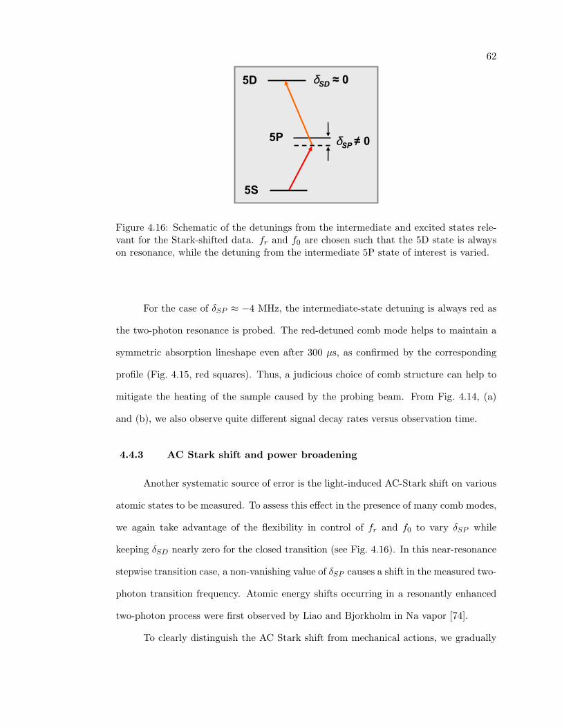
62
5P
5D
5S
δSP ≠ 0
δSD ≈ 0
Figure 4.16: Schematic of the detunings from the intermediate and excited states rele-vant for the Stark-shifted data. fr and f0 are chosen such that the 5D state is alwayson resonance, while the detuning from the intermediate 5P state of interest is varied.
For the case of δSP ≈ −4 MHz, the intermediate-state detuning is always red as
the two-photon resonance is probed. The red-detuned comb mode helps to maintain a
symmetric absorption lineshape even after 300 µs, as confirmed by the corresponding
profile (Fig. 4.15, red squares). Thus, a judicious choice of comb structure can help to
mitigate the heating of the sample caused by the probing beam. From Fig. 4.14, (a)
and (b), we also observe quite different signal decay rates versus observation time.
4.4.3 AC Stark shift and power broadening
Another systematic source of error is the light-induced AC-Stark shift on various
atomic states to be measured. To assess this effect in the presence of many comb modes,
we again take advantage of the flexibility in control of fr and f0 to vary δSP while
keeping δSD nearly zero for the closed transition (see Fig. 4.16). In this near-resonance
stepwise transition case, a non-vanishing value of δSP causes a shift in the measured two-
photon transition frequency. Atomic energy shifts occurring in a resonantly enhanced
two-photon process were first observed by Liao and Bjorkholm in Na vapor [74].
To clearly distinguish the AC Stark shift from mechanical actions, we gradually

63
(a)
Ramp Power
Time (µs)Mea
sure
dEx
pect
ed li
ne c
ente
r (kH
z)-
0 20 40 60 80 100-100
-50
0
50
100
150
200
0 MHz +4 MHz-4 MHz
δSP
(b)
3.0
2.5
2.0
1.5
1.0
Line
wid
th (F
WH
M, M
Hz)
12080400
0 MHz+ 4 MHz- 4 MHz
δSPRamp Power
Time (µs)
Figure 4.17: Measurement of (a) the line center frequency and (b) linewidth for theclosed two-photon transition, revealing frequency shifts from both the AC Stark effectand mechanical action. Extrapolating to zero interrogation time and zero power yieldsthe corrected atomic transition frequencies (a) and the natural transition linewidths (b).

64
increased the power of the pulses as the laser shutter opened. For both δSP = +4
MHz (blue triangles) and δSP = −4 MHz (red squares) cases, the AC Stark shifts are
present as soon as the laser is turned on and the transition frequency shift follows the
time evolution of the peak power of the pulse train [Fig. 4.17(a)]. When δSP = 0
MHz (black circles), the measured AC Stark shift is close to zero when the shutter just
opens. The frequency shift measured at later times is attributed to the accumulated
photon momentum transfer, which is reduced in the detuned cases. The asymmetry in
frequency shift between the red and blue detunings is caused by the presence of other
5P hyperfine states that also perturb the 5S-5D transition.
Although the laser spectrum spans roughly 26 THz, the obtained spectroscopic
resolution approaches the atomic natural linewidth. This level of resolution is a result
of the use of ultracold atoms and careful control of the phase-stabilized comb parame-
ters, stray magnetic fields, light-induced shifts, and photon-momentum transfer. We
typically measure two-photon linewidths on the order of 1 MHz [Fig. 4.17(b)], which
is roughly consistent with the convolution of the natural linewidth of 660 kHz and the
laser technical linewidth of 300 kHz. (Note that the laser linewidth is 600 kHz for a
two-photon transition.) The measured transition linewidth is slightly smaller for red
detuning (δSP = −4 MHz) than blue detuning (at the same δSP value) with the same
probe power.
4.4.4 Nulling stray magnetic fields
A direct consequence of the previous two sections is that for all the spectroscopy
experiment, the line-center values are extrapolated to zero interrogation time to suppress
shifts associated with photon-momentum transfer and the transitions are probed on
optimal resonance (i.e., zero detuning for both the intermediate state and the final
state) to minimize the AC Stark shifts.
Additionally, stray magnetic fields are minimized by applying bias-coil compen-

65
sation in three orthogonal directions. To null the residual magnetic fields we make use
of the two-photon signal itself: Zeeman-shifted spectra are obtained with right and left
circularly polarized femtosecond comb light along each direction and the zero-frequency
shift point is determined within ± 20 kHz, as presented in Fig. 4.18.
-0.4 -0.2 0.0 0.2 0.4 Magnetic Field at the MOT (Gauss)
1 MHz
Zeem
an S
hift
σ+
σ-
Figure 4.18: The two-photon fluorescence signal is used to cancel the residual mag-netic fields: Zeeman-shifted spectra are obtained with right and left circularly polarizedfemtosecond comb light and the zero-frequency shift point is determined.
4.5 Conclusion
Because the use of the femtosecond comb is novel as a direct spectroscopic probe,
in this chapter we carefully characterized several prominent systematic effects. Indeed,
the dominant effects are the mechanical action of the optical comb on the atomic motion,
the light shift induced by the probe laser, and the Zeeman frequency shifts. Now that we
have isolated the biggest contributions to the systematic line center shift and linewidth
we can actually do precision spectroscopy! In fact, the bandwidth associated with the
femtosecond pulse is sufficiently broad so that many fine and hyperfine atomic states
can be excited by tuning the relevant comb components into resonance.
Chapter 5
Two-photon absolute frequency measurements
One desirable objective in atomic spectroscopy is the ability to obtain a global
energy level picture of the atomic transitions. In fact, the stabilized comb has tremen-
dous possibilities for mapping numerous transitions in a straightforward way. In this
chapter, I will show that it is possible to obtain all of the allowed single- and two-photon
transitions within the laser bandwidth by a quick scan of fr (∼ 26 Hz). This scanning
method is efficient and eliminates the need for broadly tunable and absolutely refer-
enced cw lasers. This is one of the main advantages of using a frequency comb directly
for spectroscopy.
Previously, in Chapter 4, we scanned f0 and kept fr locked in order to characterize
the primary contributions to systematic effects on both the line center and the linewidth.
When these results are integrated into the the setup we have a system which can perform
precision mesurements. In this chapter, I focus on some representative 5S-5D transitions
for precision spectroscopy. Indeed, the measurement results approach the accuracy of
those obtained in the best cw measurements to date.
Also, if we consider that we have locked the Ti:S comb to a commercial cesium
clock and thus have generated an absolutely referenced set of optical frequencies, we
can use these frequencies for identification of previously unmeasured transitions. As
an example, we determine the previously unmeasured absolute frequency of the 5S-7S
two-photon resonances. We thus demonstrate that prior knowledge of atomic transition

67
frequencies is not essential for this technique to work, and indicate that it can be applied
in a broad context.
5.1 Scanning fr gives a full spectrum
In general, sweeping fr has the advantage of yielding all the transitions within
the laser bandwidth in only a ∼ 26 Hz scan. This is due to the fact that the ratio of one-
photon optical transition frequencies (participating in stepwise two-photon transitions)
to fr is ∼ 3.8× 10⁶, so that for a change in fr of ∼ 26 Hz the resonant enhancement is
repeated by the next neighboring comb component.
However, the optical frequency for the two-photon transitions is ∼ 770 THz, an
fr harmonic on the order of 7.7 × 10⁶. Therefore, the two-photon resonance condition
is satisfied every time fr is changed by ∼ 13 Hz, corresponding to a change in the comb
frequency by fr /2 for the mode orders around 3.85× 10⁶.
As an aside, I will discuss the two primary differences between scanning fr and
scanning f0: (i) simply stated, fr has the advantage of being multiplied by N , whereas
f0 does not and (ii) scanning fr can easily tune over 100 MHz in the optical region,
whereas scanning f0 in the current configuration produces a 80 MHz sweep at the
maximum. The trouble with scanning f0 is that the beat can reside anywhere between
0 MHz and fr/2 (there is of course a conjugate beat in the fr/2 to fr window) but,
in order for us to lock f0, we are restricted to the 7-47 MHz range. Thus, to obtain
broader tunability in the current experimental configuration, we scan f0 up to 47 MHz,
then change the sign within the servo to acquire lock on the conjugate beat and finally,
we proceed to scan this conjugate beat up to -47 MHz. This gives a total tuning of 80
MHz. (Note that we can adapt the current setup, for example by including acousto-
optic modulators in the ν-to-2 ν interferometer, to obtain continuous tuning without
having to change the servo sign.)
Figure 5.1 presents the two-photon transition spectrum obtained by scanning
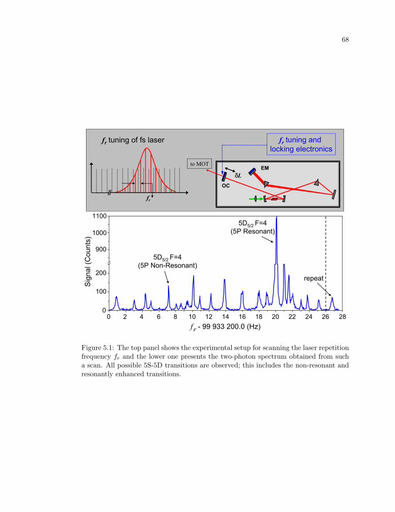
68
fr tuning of fs laser
fr
to MOT
OC
EMδL
fr tuning and locking electronics
5D5/2 F=4(5P Resonant)
5D5/2 F=4(5P Non-Resonant)
repeat
- 99 933 200.0 (Hz)rf0 2 4 6 8 10 12 14 16 18 20 22 24 26 28
0
100
200
900
1000
1100
Sign
al (C
ount
s)
Figure 5.1: The top panel shows the experimental setup for scanning the laser repetitionfrequency fr and the lower one presents the two-photon spectrum obtained from sucha scan. All possible 5S-5D transitions are observed; this includes the non-resonant andresonantly enhanced transitions.
69
fr for a fixed value of f0. It shows the 14 transitions (there are 39 possible pathways
for the case of linearly polarized light) that I identified for the 5S1/2 → 5D3/2 and
5S1/2 → 5D5/2 two-photon resonances. The data clearly show that the larger, one-
photon resonantly enhanced peaks repeat after a change of fr by ∼ 26 Hz, as expected
from the simple calculation above. As mentioned in section 4.2, for the resonantly
enhanced peaks, the pair of comb modes that is actually tuned onto the 5S-5P and
5P-5D resonances makes the dominant contribution to the two-photon transition rate.
In Fig. 5.2, we also present the theoretical spectrum corresponding to the set of
parameters used in the experiment. The two insets show signal magnitude on a loga-
rithmic scale to enhance the visibility of the smaller peaks. The peak corresponding to
non-resonant excitation of the 5S1/2 (F = 2)→ 5P3/2 (F′=3)→ 5D5/2 (F′′=4) transition,
made possible by the collective action of many comb modes, is larger than that theoreti-
cally predicted because the comb spectral phase is not flat and the comb spectrum is not
symmetric around the P state; thus, the destructive interference mentioned earlier in
section 4.2 is reduced. Furthermore, as the detuning from the P state becomes greater
than a few THz, the effect of phase mismatching between comb pairs over the spatial
dimension of the MOT can be non-negligible.
There are a couple of interesting spectral features that we notice when looking at
Fig. 5.2. The two resonance peaks observed in the experimental spectrum, which are not
present in the theory model, are due to the 5S1/2 → 7S1/2 two-photon transitions. Their
observation prompted us to consider both their theoretical modeling and experimental
investigation. However, it is more complicated to include these transitions in the model
than to include the 5S-5D two-photon transitions, primarily because their frequency has
never been measured before. In fact, this led us to actually experimentally measure their
absolute frequencies, as presented in section 5.3. I had not initially intended to study
them, though this shows again one of the powerful features of our direct frequency comb
technique, the fact that we can observe all the transitions within the fs laser bandwidth.

70
-99
933
200.
0 (H
z)rf
1280
Pul
ses
2720
Pul
ses
Step
-wis
e:S 1
/2 F
=2→
P 3/2
F=3
→D
5/2
F=4
Non
-res
onan
tS1/
2 F=
2→
D5/
2 F=
4
5S →
7S
first
pea
k re
peat
ed
1280
Pul
ses
2720
Pul
ses
5S →
7S
02
46
810
1214
1618
2022
2426
281086420
Theory (a.u.)
0246810Experiment (a.u.)
Log ScaleLog Scale
Fig
ure
5.2:
Exp
erim
enta
l(t
op)
and
sim
ulat
ed(b
otto
m)
two-
phot
onsp
ectr
aob
tain
edw
ith
afr
eque
ncy
scan
off r
.Sh
iftin
gf r
by26
Hz
shift
sth
eco
mb
spec
trum
by10
0M
Hz,
orf r
,ap
prox
imat
ely
repe
atin
gth
eor
igin
alco
mb
stru
ctur
e.T
hech
ange
sin
rela
tive
peak
size
sfr
omth
esp
ectr
umob
tain
edaf
ter
1280
puls
es(i
nre
d)to
that
afte
r27
20pu
lses
(in
blue
)ill
ustr
ate
popu
lati
ontr
ansf
erdy
nam
ics
byop
tica
lpu
mpi
ngas
wel
las
heat
ing
effec
ts.
Tw
ore
sona
nces
inth
eda
tadu
eto
the
5S→
7Str
ansi
tion
sar
eno
tin
clud
edin
our
mod
el.

71
For this fr scan, the initial ground-state population is in F=2. At longer times
(blue curves), all the transitions starting on F=2 are decreasing in amplitude compared
to shorter time scales (red curves) due to ground-state population redistribution and
heating. Most of the F=1 peaks remain unchanged or become larger. Our density
matrix simulation accounts for the time dependence of the shutter response and optical
pumping dynamics, but does not include any heating effects. The signal size shown in
Fig. 5.2 has been normalized against the square of the probe power. Not surprisingly,
both theory and experiment reveal that the most dominant transition pathway is the
closed 5S1/2 (F=2)→ 5P3/2 (F′=3) → 5D5/2 (F′′=4) transition.
The relative size of the features in Fig. 5.2 after any fixed number of pulses
reflects intermediate-state resonant enhancement as well as population transfer. Thus,
the spectrum contains all of the fine and hyperfine structure pertinent to the 5D states.
5.2 Absolute frequency measurements
After accounting for the systematics discussed in Chapter 4, we have analyzed
spectra similar to the ones shown in Fig. 5.2 to construct a table of absolute transition
frequencies from 5S to 5D (see Table 5.1). We isolated the five two-photon transitions
which start in F=2, and go through 5P3/2 F′=3, i.e. two-photon transitions which have
the 5S-5P step as a closed transition. This closed first step may help with the optical
pumping, giving better signal-to-noise ratios to determine their absolute frequency.
These representative transition frequencies are determined directly from the comb
structure and are given in the table, along with comparisons to available published
values [75]. The measurement accuracy is currently a few kHz to a few tens of kHz for
the 5D states and on the order of 100 kHz for the 5P states, comparable to the highest
resolution measurements made with cw lasers. All the measurement errors reported
here are statistical errors (one standard deviation of the mean).

72
Measured transition Measured frequency (kHz) Literature value (kHz)5S1/2 F=2→ 5D5/2 F′′=2 770 569 184 527.9 (49.3) 770 569 184 510.4 (16.0)5S1/2 F=2→ 5D5/2 F′′=3 770 569 161 560.5 (11.1) 770 569 161 555.6 (16.0)5S1/2 F=2→ 5D5/2 F′′=4 770 569 132 748.8 (16.8) 770 569 132 732.6 (16.0)5S1/2 F=2→ 5D3/2 F′′=3 770 480 275 633.7 (12.7) 770 480 275 607.6 (10.0)5S1/2 F=2→ 5D3/2 F′′=2 770 480 231 393.9 (38.1) 770 480 231 385.2 (10.0)5S1/2 F=2→ 7S1/2 F′′=2 788 794 768 921.4 (44.5) 788 794 768 878.0 (40.0)5S1/2 F=1→ 7S1/2 F′′=1 788 800 964 199.3 (121.9) 788 800 964 042.0 (40.0)
Table 5.1: 87Rb level structure from direct frequency comb spectroscopy. All the valuesare obtained by extrapolating the line center to zero probing time and power. The firstsix transitions presented here are resonantly enhanced by the 5P3/2 F′=3 state and thushave a closed first step. The final seventh transition passes through the 5P3/2 F′=1intermediate level.
We will now move on to discuss the measurement of the two extra resonances
that appeared in the spectra shown in Fig. 5.2.
5.3 5S-7S absolute frequency measurements
After observing the two resonances, we reviewed the literature and discovered
that in fact no one had measured these transitions with high precision. Without a
priori information of the 7S energy levels, we have determined their absolute transition
frequencies [76]. We have used the transition wavelength reported in the online NIST
atomic database, which was of course covered by the fs laser spectrum, so we were able
to determine the resonance frequencies. A single optical comb thus provides atomic
structural information in the optical, terahertz, and radio-frequency spectral domains.
I will discuss in some detail now the 5S-7S two-photon frequency measurements.
They were performed in a similar manner to the 5S-5D measurements, with the im-
portant change that we used a Pockels cell with a 8-ns rise time instead of the liquid
crystal shutter (∼ 30 µs response time). As a consequence, we did not have to account
for the shutter turn-on when obtaining the final frequency values, which made it eas-
ier to extrapolate to zero power. The experiment cycle and general method remained

73
the same, especially since the 7S levels also decay through the 6P levels, which means
that we were able to use the same PMT. As seen from the general frequency diagram
in section 4.2, the wavelengths for the second step of the resonantly enhanced 5S-7S
transitions are 741 nm for transitions via 5P3/2 and 728 nm for transitions via 5P1/2.
The energy degenerate two-photon transition is at 760 nm. This makes it more difficult
to cover them in our spectrum, optimized for 778 nm. This fact is especially true about
728 nm wavelength. Shifting the spectrum to smaller wavelengths is definitely doable,
the problem is having a sufficient signal-to-noise ratio for the f0 beat to properly main-
tain phase-lock of the Ti:S. The degradation in the signal-to-noise ratio of the f0 beat
occurs because the microstructure fiber is optimized for its zero GVD point near 800
nm. Thus, I usually center the fs spectrum at 770 nm for these measurements and I try
to use only transitions enhanced by a 5P3/2 intermediate level.
Shown in Fig. 5.3(a) is a typical 7S1/2 F′′=2 Lorentzian lineshape, generated by
stepping the offset frequency f0 for a fixed value of the repetition rate fr and recording
the subsequent blue fluorescence corresponding to the 7S population. For each data
point, to obtain a better signal-to-noise ratio, the 80 ns-binned counts arising from the
fluorescence are integrated over 2.4 µs. Alternatively, this lineshape is retrieved by
sweeping fr with f0 fixed at some convenient value.
Once the lineshape has been acquired, what remains is to identify the correct
mode number N associated with each transition. If the optical frequency is already
known to within fr/2, this is a straightforward task. For the case of the 5S-7S two-
photon transitions, where the resonance frequencies are not known a priori (νopt = (N1+
N2)fr + 2f0), we scan the resonances for two different values of fr and unambiguously
deduce the sum of the two associated integers (N1 + N2) [77, 78]. In our case, the two
repetition rates used are separated by 600 kHz to eliminate possible uncertainties arising
from estimations of the f0 value corresponding to the peak of the resonance.
After identifying the comb numbers associated with the transition and reducing

74
1.0
0.8
0.6
0.4
0.2
0.024222018
Data Fit
7S1/2 Lineshape
Sig
nal (
a.u.
)
f0 (MHz)
(a)
1500
1000
500
0806040200
Mea
sure
d
ν (k
Hz)
Probing Time (µs)
Line center shift Fit
ν = 788 794 768 921 kHz
(b)0
0
Figure 5.3: (a) Typical 5S1/2 F=2→ 7S1/2 F′′=2 two-photon Lorentzian lineshape ob-tained from a scan of the offset frequency f0 for a fixed value of the repetition rate fr .For each data point, the 80 ns-binned counts arising from the fluorescence are integratedover 2.4 s. (b) Frequency shift of the transition line center vs. probing time resultingfrom the momentum transferred by the femtosecond laser to the cold 87Rb atoms. Ex-trapolation to zero interrogation time gives absolute atomic transition frequencies, aswell as roughly the natural linewidth, free of radiation pressure effects.
the systematic error arising from AC Stark shift (by probing on optimal resonance i.e.,
zero detuning for both the intermediate state and the final state), the remaining error
from radiation pressure is suppressed by extrapolating to zero interrogation time, as

75
shown in Fig. 5.3(b). We determine for the 5S1/2 F=2→ 7S1/2 F′′=2 and the 5S1/2 F=1
→ 7S1/2 F′′=1 two-photon transitions in 87Rb the absolute optical frequencies of 788 794
768 921(44) kHz and 788 800 964 199 (122) kHz, respectively (see Table 5.1). The excited
state hyperfine interval of 639 404 (130) kHz agrees very well with a previous differential
measurement performed with a picosecond pulsed laser [70]. The transition spectra
reported in [70], as well as a continuous-wave (cw) laser-based scan [79], indicated
that the F=2 → F′′=2 and the F=1 → F′′=1, i.e. ∆F=0 transitions, were the only
allowed 5S-7S transitions in 87Rb. However, we observe additional lines, as the resonant
intermediate 5P state also enables the F=2 → F′′=1 and F=1 → F′′=2, i.e., ∆F=±1,
two-photon transitions. Similar ∆F=±1 S-S transitions have been previously observed
in Na in a two-step excitation experiment employing two tunable cw dye lasers, which
enabled a direct measurement of the excited state hyperfine splitting [80].
We recently learned that conventional, cw laser-based measurements of the 5S-7S
transitions in Rb were reported by Chui et al. [81]. Our measurements agree with their
results, within one standard deviation of the mean for the reported values, as can be
seen from Table 5.1. Thus, we have demonstrated that by using DFCS, the absolute
value of the 5S1/2 → 7S1/2 two-photon transitions in 87Rb is conclusively determined,
with no a priori knowledge about their optical frequency.
In the next chapter I will discuss single-photon frequency measurements that
we recently made. As described there, one indirect way to determine the absolute
frequencies of the 5S-5P transition is to scan the 5P state by using a set of fr and f0 pairs
that have a range of detunings from the 5P state and are all two-photon resonant. I will
show that detailed dynamics of population transfer driven by a sequence of pulses have
to be taken into account for the measurement of the 5P states via resonantly enhanced
two-photon transitions.

Chapter 6
One-photon absolute frequency measurements
Direct Frequency Comb Spectroscopy (DFCS) can be equally well applied to
measure single-photon transitions. However, since we have the ability to dynamically
access two-photon transitions (as shown in Chapter 4), we can measure the energy
of a given state in two ways. We can either investigate an atomic state as part of a
one-photon process or as a two-photon process. We have chosen the 5S-5P transitions
in 87Rb to demonstrate this ability. The measurement of 5P states has been carried
out directly and also indirectly, via the 5S-5D two-photon transitions by studying their
resonant enhancement when comb components are scanned through the intermediate
5P states. We compare the 5P measurements obtained via one-photon and two-photon
DFCS and clearly demonstrate the importance of population transfer in working with
multilevel systems probed by multiple comb components.
Also, again with the technique of DFCS, we have the advantage of being able to
determine absolute atomic transition frequencies anywhere within the comb bandwidth,
for one-photon processes.
6.1 Detection and timing scheme for the direct 5P measurements
For the one-photon studies we have investigated both the D1 and D2 transitions
in 87Rb, namely transitions from the ground state to the 5P1/2 excited state at 795 nm
and to the 5P3/2 state at 780 nm (see general diagram, in section 4.2).
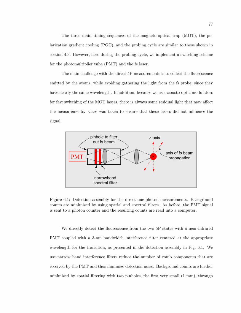
77
The three main timing sequences of the magneto-optical trap (MOT), the po-
larization gradient cooling (PGC), and the probing cycle are similar to those shown in
section 4.3. However, here during the probing cycle, we implement a switching scheme
for the photomultiplier tube (PMT) and the fs laser.
The main challenge with the direct 5P measurements is to collect the fluorescence
emitted by the atoms, while avoiding gathering the light from the fs probe, since they
have nearly the same wavelength. In addition, because we use acousto-optic modulators
for fast switching of the MOT lasers, there is always some residual light that may affect
the measurements. Care was taken to ensure that these lasers did not influence the
signal.
PMTaxis of fs beam
propagation
z-axispinhole to filterout fs beam
narrowbandspectral filter
Figure 6.1: Detection assembly for the direct one-photon measurements. Backgroundcounts are minimized by using spatial and spectral filters. As before, the PMT signalis sent to a photon counter and the resulting counts are read into a computer.
We directly detect the fluorescence from the two 5P states with a near-infrared
PMT coupled with a 3-nm bandwidth interference filter centered at the appropriate
wavelength for the transition, as presented in the detection assembly in Fig. 6.1. We
use narrow band interference filters reduce the number of comb components that are
received by the PMT and thus minimize detection noise. Background counts are further
minimized by spatial filtering with two pinholes, the first very small (1 mm), through

78
which the MOT is imaged [Fig. 6.1]. Photon collection during the probe laser-on period
is disabled by switching off the PMT.
The loading cycle used for the MOT is 100 Hz, and the sequence of the experiment
is similar to the two-photon experiments [Fig. 6.2]: the atoms are loaded in the MOT
for 7.8 ms, then the quadrupole magnetic field for the trap is switched off, the atoms are
cooled with polarization gradients for 2 ms, then all the MOT beams are extinguished
and the femtosecond comb beam is switched on for 200 µs using the Pockels cell (8-ns
rise time)
As illustrated in the one-photon timing diagram in Fig. 6.2, during the 200 µs
probe window, we have a sequence of short cycles with the probe laser on (200 ns)
followed by the PMT on (400 ns) to detect photons from the fast-decaying 5P states. A
2.6 µs interval (PMT switch-off time) is required before initiating the next laser cycle.
Both the two-photon and the single-photon signals are averaged over hundreds of 10 ms
experiment cycles.
MOT7.5 ms
PGC2 ms
tOne-photon
timing diagram
200 µs
400 ns, PMT on200 ns, fs on
...
Figure 6.2: Timing scheme for the 100 Hz experiment cycle, where the 200-µs zoomwindow shows the sequences for the direct one-photon measurements. We switch thePMT off during the laser-on period, to minimize detection noise.
For the indirect 5P measurements, we use results from the theoretical model
describing the fs comb interaction with the atoms. As discussed in Chapter 2, the

79
theory accounts for detailed dynamics of population transfer among the atomic states
involved in transitions within the comb bandwidth. A numerical scheme is employed
to obtain the state of the atomic system after an arbitrary number of pulses [37, 60].
This model is applied to accurately predict the coherent population accumulation in the
relatively long-lived 5D, followed by incoherent optical pumping. Especially important
for the indirect 5P measurements is the incoherent optical pumping to the ground state
hyperfine levels, which depends critically on the 5P state detunings and will be discussed
in detail below.
We will now compare one-photon and two-photon DFCS measurements for the
5P state energy levels. The one-photon DFCS employs radiative detection directly from
the 5P states (Fig. 6.3, left panel), while the two-photon DFCS studies the 5P states
indirectly, via resonant enhancement of the 5S-5D two-photon transitions as a function
of the detuning from the intermediate 5P states (Fig. 6.3, right panel).
F=2F=15S
5P
PMTF=2F=1
5D
5P
5S
6P
PMT
one-photonDFCS
two-photonDFCS
Figure 6.3: Schematic of one- and two-photon DFCS, used for measuring single-photontransition frequencies. The two-photon DFCS here differs from the two-photon processdescribed in Chapter 5 in that the 5D state is kept strictly in resonance. The 5Plineshape is obtained by scanning the detuning.

80
6.2 5P3/2 frequency measurements
First, we measure the 5S1/2 F=2 → 5P3/2 F′=3 D2 transition with one-photon
DFCS, with the resulting transition line shown in Fig. 6.4(a) [76]. Frequency scans are
carried out similarly to those of the 5S-5D lines, that is, by stepping f0 continuously
while keeping fr fixed. The absolute optical frequency measured for this transition is
384 228 115 271 (87) kHz, in agreement with a previous measurement done here at
JILA [82], which resulted in an absolute frequency value of 384 228 115 203 (7) kHz.
Once again, all the measurement errors reported in this chapter, and actually in this
thesis, are statistical errors (one standard deviation of the mean).
For the two-photon DFCS, we use a set of different pairs of fr and f0 specifi-
cally chosen to have varying detunings from the 5P state for each data point shown in
Fig. 6.4(b), while at the same time satisfying strictly the 5S-5D two-photon resonance
(δSD = 0). In this case, we monitor once again the 420 nm fluorescence from the 5D
states. Such a set of fr and f0 is given as an example in Table 6.1. We immediately
see that fr must be known within 10 mHz. To obtain this level of accuracy, we always
reference the fr frequency counter to the cesium clock in our lab. As mentioned earlier,
this is necessary because the fr excursions get multiplied by ∼ 8 × 10⁶. In contrast,
f0 must only be stable within 100 Hz.
The lineshape in Fig. 6.4(b) is retrieved by detecting the 420 nm signal as a
function of 5P state detuning and the optical frequency measured by this two-photon
DFCS is 384 228 115 309 (63) kHz, in agreement with the result obtained from one-
photon DFCS within the standard deviation. Although the two methods for measuring
this 5P state, direct and indirect, agree well, the indirect one is more cumbersome for
two main reasons. Firstly, fr must be changed by such a large amount as to require
the output coupler to be placed on a translation stage and thus, the laser box to be
opened for each detuning value. Secondly, this required hand-tuning adds significant

81
1.0
0.8
0.6
0.4
353025201510
Data Fit
Single-photon P3/2
f0 (MHz)Si
gnal
(a.u
.)
(a)
1.0
0.8
0.6
0.4
0.2
0.0-10 0 10
Data Fit
P3/2 lineshape via a two-photon scan
Sign
al (a
.u.)
5P State Detuning (MHz)
(b)
Figure 6.4: (a) Lineshape of the 5S1/2 F=2→ 5P3/2 F′=3 transition obtained from ascan of f0 for a fixed value of fr, by one-photon DFCS. (b) Same lineshape as in (a),retrieved using its resonant enhancement of the 5S1/2 F=2→ 5P3/2 F′=3→ 5D5/2 F′′=4closed two-photon transition, as a function of the detuning from the intermediate state.
time for retrieving a lineshape, so it is important that the data be taken under the same
conditions and thus, it all has to be acquired on the same day. The direct method,
though requiring an extra (switched) PMT, allows for a fast and smooth scan of the 5P
states.
It is also important to mention that for this scan we take advantage of the
5S1/2 F=2 → 5P3/2 F′=3 → 5D5/2 F′′=4 being the only 5S-5D closed transition.
As shown in the theory plots in Fig. 6.5, this closed transition ensures that most of

825P detuning (MHz) fr (MHz) f0 (MHz)
-13 99.89260605 -16.4737-10 99.92066423 -22.4503-9 99.93474869 -16.2599-4 99.92482030 -9.9189-3 99.93890785 -11.1280-2 99.91518350 -21.3653+1 99.94325356 -24.2433+3 99.86747878 -22.2673+4 99.88155032 -24.0872+5 99.89562280 -14.1944+9 99.84803930 -11.4370+12 99.84303590 -24.3973
Table 6.1: Example of a set of fr and f0 pairs used for the indirect scanning of theintermediate 5P3/2 F′=3 state. All the detunings are given with respect to this P state.The values for fr and f0 are chosen to ensure that the F′′=4 state is always resonantfor this indirect scan.
1.0
0.8
0.6
0.4
0.2
0.01086420
F=2, +4 MHz detuning F=2, -4 MHz detuning
F=1, -4 MHz detuning F=1, +4 MHz detuning
Time (µs)Frac
tiona
l Gro
und
Stat
e Po
pula
tion
Figure 6.5: Theoretical plot of the time evolution of the ground state populations fortwo (symmetric) detuning values in Fig. 6.4(b), showing that (i) most of the atomsremain in the initial F=2 ground level for this closed two-photon transition and (ii) theground state populations are largely insensitive to the sign of the detuning.
the atoms initially starting out in the F=2 ground-state hyperfine level remain in that
level, while ∼20% of the atoms fall into the dark F=1 ground state due to optical
pumping and hence do not contribute to the signal. In addition, the probe laser power
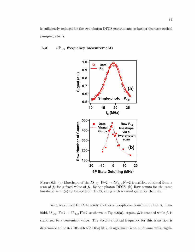
83
is sufficiently reduced for the two-photon DFCS experiments to further decrease optical
pumping effects.
6.3 5P1/2 frequency measurements
1.0
0.9
0.8
0.7
0.6
0.525201510
Single-photon P1/2
f0 (MHz)
Sign
al (a
.u)
Data Fit
(a)
500
400
300
200
100-20 -10 0 10 20
Data Visual
Guide
Raw P1/2
lineshape via atwo-photon scan
5P State Detuning (MHz)
Raw
Num
ber o
f Cou
nts
(b)
Figure 6.6: (a) Lineshape of the 5S1/2 F=2 → 5P1/2 F′=2 transition obtained from ascan of f0 for a fixed value of fr, by one-photon DFCS. (b) Raw counts for the samelineshape as in (a) by two-photon DFCS, along with a visual guide for the data.
Next, we employ DFCS to study another single-photon transition in the D1 man-
ifold, 5S1/2 F=2 → 5P1/2 F′=2, as shown in Fig. 6.6(a). Again, f0 is scanned while fr is
stabilized to a convenient value. The absolute optical frequency for this transition is
determined to be 377 105 206 563 (184) kHz, in agreement with a previous wavelength-

84
based measurement [83], which gave an absolute frequency value of 377 105 206 705
(400) kHz for this transition.
For the corresponding two-photon DFCS experiment we map the 5S1/2 F=2
→ 5P1/2 F′=2 → 5D3/2 F′′=3 two-photon transition in the same manner employed for
Fig. 6.4(b). Figure 6.6(b) shows the raw data yielded by the (fr, f0) pair selections,
along with a visual guide for the data. The apparent linewidth is significantly broader
than that associated with the 5P state.
Unlike the previous two-photon DFCS measurement reported in Fig. 6.4, the
pairs of fr and f0 used to obtain each point in Fig. 6.6(b) lead to substantially different
detunings of the other 5P states and subsequently, varying optical pumping to the F=1
ground state. Indeed, the theory model applied to the actual experiment conditions
predicts significantly different ground state population transfer dynamics. As shown in
Fig. 6.7, the asymptotic values of the F=2 ground-state population are not the same
for symmetric detunings from the intermediate state.
1.0
0.8
0.6
0.4
0.2
0.01086420
F=1, +4 MHz detuning F=1, -4 MHz detuning
F=2, -4 MHz detuning F=2, +4 MHz detuning
Time (µs)Frac
tiona
l Gro
und
Stat
e Po
pula
tion
Figure 6.7: Theoretical plot of the time evolution of the ground state populations for two(symmetric) detuning values in 6.6(b), showing a significant difference in the populationtransfer between the ground state levels due to optical pumping caused by varyingdetunings from the other 5P states.
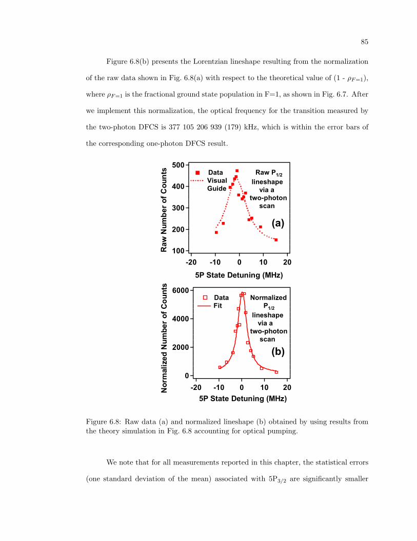
85
Figure 6.8(b) presents the Lorentzian lineshape resulting from the normalization
of the raw data shown in Fig. 6.8(a) with respect to the theoretical value of (1 - ρF=1),
where ρF=1 is the fractional ground state population in F=1, as shown in Fig. 6.7. After
we implement this normalization, the optical frequency for the transition measured by
the two-photon DFCS is 377 105 206 939 (179) kHz, which is within the error bars of
the corresponding one-photon DFCS result.
6000
4000
2000
0-20 -10 0 10 20
Normalized P1/2
lineshape via a two-photon scan
Data Fit
5P State Detuning (MHz)
Nor
mal
ized
Num
ber o
f Cou
nts
(b)
500
400
300
200
100-20 -10 0 10 20
Data Visual
Guide
Raw P1/2
lineshape via atwo-photon scan
5P State Detuning (MHz)
Raw
Num
ber o
f Cou
nts
(a)
Figure 6.8: Raw data (a) and normalized lineshape (b) obtained by using results fromthe theory simulation in Fig. 6.8 accounting for optical pumping.
We note that for all measurements reported in this chapter, the statistical errors
(one standard deviation of the mean) associated with 5P3/2 are significantly smaller

86
than those associated with 5P1/2. This is due to the stronger transition strength and
less severe optical pumping effects for 5P3/2 F′=3 (part of a closed transition), leading
to larger signal-to-noise ratios.
Direct frequency comb measurements of one-photon transitions in atoms other
than 87Rb have been recently reported. In Leo Hollberg’s group at NIST, they probed
Cs in an atomic beam with DFCS, but using a Ti:S laser with a 1 GHz repetition
rate [84]. Employing a 1-GHz fs laser has several advantages over a lower fr laser, as
stated in Chapter 7.
In conclusion, a phase-stabilized femtosecond comb has been used as an effective
tool to perform direct spectroscopy of one-photon transitions in cold 87Rb atoms. We
have demonstrated that DFCS can be successfully applied to one-photon studies, by
measuring 5S1/2 → 5P1/2,3/2 transitions both directly and indirectly, via their resonant
enhancement of the 5S-5D two-photon transitions. Additionally, we have shown the
importance of including the dynamic population changes arising from pulse-accumulated
population transfer in this indirect one-photon measurement.

Chapter 7
Summary and outlook
In this thesis, we have joined together the study of cold atoms, which are well
established as an ideal sample for spectroscopy with the field of ultrafast lasers, which
have recently emerged as a powerful tool for frequency metrology.
We have used a wide-bandwidth, phase-stabilized femtosecond laser as a novel
and efficient tool to perform Direct Frequency Comb Spectroscopy (DFCS) of one-
photon and two-photon transitions in laser-cooled 87Rb atoms. To begin with, we have
studied the dominant sources of systematic shifts and tried to reduce their effects as
much as possible. We have then measured the absolute atomic frequency for several
5S1/2 → 5D3/2,5/2 two-photon transitions in 87Rb. The two-photon spectroscopy is car-
ried out efficiently despite the low laser power, because we take advantage of intermedi-
ate 5P states that are near-resonant with a comb line. We have demonstrated that the
absolute optical frequency of the previously unmeasured 5S1/2 → 7S1/2 resonances can
be determined unambiguously from the comb structure used in the experiment. Lastly,
we have shown that DFCS can be successfully applied to one-photon processes as well,
by measuring 5S1/2 → 5P1/2,3/2 transitions both directly and indirectly, through their
resonant enhancement of the 5S-5D two-photon transitions. Detailed dynamics of popu-
lation transfer driven by a sequence of pulses were uncovered and taken into account for
the indirect measurement of the 5P states. Although the current experiments involve
one- and two-photon transitions, the advantages of DFCS should also apply to multi-

88
photon excitations. In general, DFCS permits global, high-resolution spectroscopy of
all the atomic transitions within the comb bandwidth.
After we successfully implemented DFCS for the study of several one- and two-
photon transitions, there is still room left for improvements. Firstly, the resolution of
DFCS can be enhanced by locking the femtosecond laser to a cavity, which has been
shown capable to reduce the linewidth to below 100 Hz [85], rather than the current 300
kHz. Secondly, a larger signal can be obtained by using a laser with a higher repetition
rate; for example, a 1-GHz laser with the same average power and spectral width could
increase the signal up to a 100-fold. This is a result of the quadratic increase of the ex-
cited state population versus the accumulated number of pulses, where the higher fr and
hence the shorter pulse interval allow for more pulses to be ‘added’ during the atomic
coherence lifetime. Additionally, the power is distributed among fewer comb lines for
this fr ∼ 1 GHz case, and the decreased congestion of lines would reduce optical pump-
ing effects. Achieving simultaneous one- and two-photon resonance conditions should
still be possible. Using a 1-GHz laser provides more latitude in identifying the mode
number of the comb component that is resonant with each optical transition. The larger
mode spacing makes this identification easier, because it only requires knowledge of the
optical frequencies with a precision of a few hundred MHz. One practical consequence
of these results is a method to control both degrees of freedom of the femtosecond comb
directly by an optical transition in cold atoms.
Another interesting application of the demonstrated pulse accumulation effect
is using ultrafast pulse trains for laser cooling of atoms (e.g. hydrogen, deuterium,
antihydrogen) that require coherent ultraviolet light not easily accessible by conven-
tional laser sources [86]. Toward this goal, an extension of frequency comb metrol-
ogy to the deep-ultraviolet spectral region (where cw lasers are not readily available)
was recently achieved using an amplified train of phase-controlled pulses from a fem-
tosecond laser [78]. The peak power of these pulses allowed for efficient harmonic

89
upconversion and thus, the 4th harmonic of the femtosecond laser was used for two-
photon spectroscopy in krypton. Even more recently, phase-coherent frequency combs
in the vacuum-ultraviolet spectral region were demonstrated in our lab, without active
amplification of the standard femtosecond laser [87]. Its output was stabilized to a
completely passive optical cavity, with a gas jet at the intracavity focus, generating a
phase-controlled frequency comb in the extreme ultraviolet region which preserves the
original repetition frequency. This technique, in combination with DFCS, opens the
door to more accurate atomic optical clocks that operate on resonances with ultrahigh,
vacuum-ultraviolet or extreme-ultraviolet, frequencies. These clocks would have a very
high stability, proportional to their transition frequency.
For general coherent control experiments, pulse accumulation (when enabled by
long coherence times) can complement spectral amplitude and phase manipulations,
leading to improved efficiency in population control with the added spectral resolution
and longer experimental timescales due to maintaining phase coherence for many con-
secutive laser pulses. The precise and phase-coherent pulse accumulation may prove
particularly useful in efficiently populating atomic Rydberg states for quantum infor-
mation processing. Multiple ultrafast lasers with optical spectra independently tailored
for different spectroscopic features could be phase coherently stitched together [9,88] to
further extend the utility of this approach.

Bibliography
[1] D. J. Jones, S. A. Diddams, J. K. Ranka, A. Stentz, R. S. Windeler, J. L. Hall, andS. T. Cundiff, “Carrier-envelope phase control of femtosecond mode-locked lasersand direct optical frequency synthesis,” Science 288, 635–639 (2000).
[2] A. Apolonski, A. Poppe, G. Tempea, C. Spielmann, T. Udem, R. Holzwarth,T. W. Hansch, and F. Krausz, “Controlling the Phase Evolution of Few-CycleLight Pulses,” Phys. Rev. Lett. 85, 740–743 (2000).
[3] H. S. Margolis, G. P. Barwood, G. Huang, H. A. Klein, S. N. Lea, K. Szymaniec,and P. Gill, “Hertz-Level Measurement of the Optical Clock Frequency in a Single88Sr+ Ion,” Science 306, 1355–1358 (2004).
[4] S. A. Diddams, T. Udem, J. C. Bergquist, E. A. Curtis, R. E. Drullinger, L. Holl-berg, W. M. Itano, W. D. Lee, C. W. Oates, K. R. Vogel, and D. J. Wineland, “Anoptical clock based on a single trapped 199Hg+ ion,” Science 293, 825–828 (2001).
[5] J. Ye, L.-S. Ma, and J. L. Hall, “Molecular iodine clock,” Phys. Rev. Lett. 87,270 801 (2001).
[6] J. D. Jost, J. L. Hall, and J. Ye, “Continuously tunable, precise, single frequencyoptical signal generator,” Opt. Exp. 10, 515–520 (2002).
[7] T. M. Fortier, D. J. Jones, and S. T. Cundiff, “Phase stabilization of an octave-spanning Ti:sapphire laser,” Opt. Lett. 28, 2198–2200 (2003).
[8] A. Baltuska, T. Fuji, and T. Kobayashi, “Controlling the Carrier-Envelope Phaseof Ultrashort Light Pulses with Optical Parametric Amplifiers,” Phys. Rev. Lett.88, 133 901 (2002).
[9] R. K. Shelton, L.-S. Ma, H. C. Kapteyn, M. M. Murnane, J. L. Hall, and J. Ye,“Phase-coherent optical pulse synthesis from separate femtosecond lasers,” Science293, 1286–1289 (2001).
[10] A. Baltuska, T. Udem, M. Uiberacker, M. Hentschel, E. Goulielmakis, C. Gohle,R. Holzwarth, V. S. Yakovlev, A. Scrinzi, T. W. Hansch, and F. Krausz, “Attosec-ond control of electronic processes by intense light fields,” Nature 421, 611–615(2003).

91
[11] T. C. Weinacht, J. Ahn, and P. H. Bucksbaum, “Controlling the shape of a quantumwavefunction,” Nature 397, 233–235 (1999).
[12] T. M. Fortier, P. A. Roos, D. J. Jones, S. T. Cundiff, R. D. R. Bhat, and J. E.Sipe, “Carrier-Envelope Phase-Controlled Quantum Interference of Injected Pho-tocurrents in Semiconductors,” Phys. Rev. Lett. 92, 147 403 (2004).
[13] E. O. Potma, D. J. Jones, J.-X. Cheng, X. S. Xie, and J. Ye, “High-sensitivitycoherent anti-Stokes Raman scattering microscopy with two tightly synchronizedpicosecond lasers,” Opt. Lett. 27, 1168–1170 (2002).
[14] D. Meshulach and Y. Silberberg, “Coherent quantum control of two-photon tran-sitions by a femtosecond laser pulse,” Nature 396, 239–242 (1998).
[15] T. Udem, J. Reichert, R. Holzwarth, and T. W. Hansch, “Accurate measurementof large optical frequency differences with a mode-locked laser,” Opt. Lett. 24,881–883 (1999).
[16] M. T. Asaki, C.-P. Huang, D. Garvey, J. Zhou, H. C. Kapteyn, and M. M. Murnane,“Generation of 11-Fs pulses from a self-mode-locked Ti-Sapphire laser,” Opt. Lett.18, 977–979 (1993).
[17] C. Salomon, D. Hils, and J. L. Hall, “Laser stabilization at the millihertz level,” J.Opt. Soc. Am. B 5, 1576–1587 (1988).
[18] T. Udem, J. Reichert, R. Holzwarth, and T. Hansch, “Absolute optical frequencymeasurement of the cesium D1 line with a mode-locked laser,” Phys. Rev. Lett.82, 3568–3571 (1999).
[19] S. A. Diddams, D. J. Jones, L.-S. Ma, S. T. Cundiff, and J. L. Hall, “Opticalfrequency measurement across a 104-THz gap with a femtosecond laser frequencycomb,” Opt. Lett. 25, 186–188 (2000).
[20] S. A. Diddams, D. J. Jones, J. Ye, S. T. Cundiff, J. L. Hall, J. K. Ranka, R. S.Windeler, R. Holzwarth, T. Udem, and T. W. Hansch, “Direct link between mi-crowave and optical frequencies with a 300 THz femtosecond laser comb,” Phys.Rev. Lett. 84, 5102–5105 (2000).
[21] H. R. Telle, G. Steinmeyer, A. Dunlop, J. Stenger, D. Sutter, and U. Keller,“Carrier-envelope offset phase control: A novel concept for absolute optical fre-quency control and ultrashort pulse generation,” Appl. Phys. B 69, 327–332 (1999).
[22] J. K. Ranka, R. S. Windeler, and A. J. Stentz, “Visible continuum generation inair-silica microstructure optical fibers with anomalous dispersion at 800 nm,” Opt.Lett. 25, 25–27 (2000).
[23] S. T. Cundiff and J. Ye, “Colloquium: Femtosecond optical frequency combs,” Rev.Mod. Phys. 75, 325–342 (2003).
[24] T. W. Hansch, Tunable Lasers and Applications, section “SpectroscopicApplications of Tunable Lasers”, A. Mooradian, T. Jaeger and P. Stokseth, Editors(Springer-Verlag, Berlin, 1976).

92
[25] R. Teets, J. Eckstein, and T. W. Hansch, “Coherent two-photon excitation bymultiple light pulses,” Phys. Rev. Lett. 38, 760–764 (1977).
[26] A. I. Ferguson, J. N. Eckstein, and T. W. Hansch, “A subpicosecond dye laserdirectly pumped by a mode-locked argon laser,” J. Appl. Phys. 49, 5389–5391(1978).
[27] J. N. Eckstein, A. I. Ferguson, and T. W. Hansch, “High-resolution two-photonspectroscopy with picosecond light pulses,” Phys. Rev. Lett. 40, 847–850 (1978).
[28] S. T. Cundiff, J. Ye, and J. L. Hall, “Optical frequency synthesis based on mode-locked lasers,” Rev. Sci. Instr. 72, 3749–3771 (2001).
[29] K. M. Evenson, J. S. Wells, F. R. Petersen, B. L. Danielson, and G. W. Day,“Accurate frequencies of molecular transitions used in laser stabilization: the 3.39-µm transition in CH4 and the 9.33- and 10.18-µm transitions in CO2,” Appl. Phys.Lett. 22, 192–195 (1973).
[30] K. M. Evenson, J. S. Wells, F. R. Petersen, B. L. Danielson, G. W. Day, R. L.Barger, and J. L. Hall, “Speed of Light from Direct Frequency and WavelengthMeasurements of the Methane-Stabilized Laser,” Phys. Rev. Lett. 29, 1346–1349(1972).
[31] D. A. Jennings, C. R. Pollock, F. R. Petersen, R. E. Drullinger, K. M. Evenson,J. S. Wells, J. L. Hall, and H. P. Layer, “Direct frequency measurement of the I2stabilized He-Ne 473-THz (633-nm) laser,” Opt. Lett. 8, 136–138 (1983).
[32] H. Schnatz, B. Lipphardt, J. Helmcke, F. Riehle, and G. Zinner, “First phase-coherent frequency measurement of visible radiation,” Phys. Rev. Lett. 76, 18–21(1996).
[33] J. E. Bernard, A. A. Madej, L. Marmet, B. G. Whitford, K. J. Siemsen, andS. Cundy, “Cs-Based Frequency Measurement of a Single, Trapped Ion Transitionin the Visible Region of the Spectrum,” Phys. Rev. Lett. 82, 3228–3231 (1999).
[34] C. Schwob, L. Jozefowski, B. de Beauvoir, L. Hilico, F. Nez, L. Julien, F. Biraben,O. Acef, and A. Clairon, “Optical frequency measurement of the 2S-12D transitionsin hydrogen and deuterium: Rydberg constant and lamb shift determinations,”Phys. Rev. Lett. 82, 4960–4963 (1999).
[35] T. H. Yoon, A. Marian, J. L. Hall, and J. Ye, “Phase-coherent multilevel two-photontransitions in cold Rb atoms: Ultrahigh-resolution spectroscopy via frequency-stabilized femtosecond laser,” Phys. Rev. A 63, 011 402(R) (2000).
[36] O. S. Heavens, “Radiative transition probabilities of the lower excited states of thealkali metals,” J. Opt. Soc. Am. 51, 1058–1061 (1961).
[37] D. Felinto, C. A. C. Bosco, L. H. Acioli, and S. S. Vianna, “Coherent accumulationin two-level atoms excited by a train of ultrashort pulses,” Opt. Commun. 215,69–73 (2003).

93
[38] D. Felinto, L. H. Acioli, and S. S. Vianna, “Accumulative effects in the coherenceof three-level atoms excited by femtosecond-laser frequency combs,” Phys. Rev. A70, 043 403 (2004).
[39] N. V. Vitanov and P. L. Knight, “Coherent excitation of a two-state system by atrain of short pulses,” Phys. Rev. A 52, 2245–2261 (1995).
[40] M. M. Salour, “Quantum interference effects in two-photon spectroscopy,” Rev.Mod. Phys. 50, 667–681 (1978).
[41] M. Stowe, “Private communication,” .
[42] Femtosecond Optical Frequency Comb Technology: Principle, Operation andApplication, J. Ye and S. T. Cundiff, Editors (Springer, New York, 2005).
[43] T. M. Fortier, “Phase Stabilized Modelocked Lasers: from optical frequency metrol-ogy to waveform synthesis of ultrashort pulses,” Ph. D Thesis, JILA and Universityof Colorado (2004).
[44] J. Reichert, R. Holzwarth, T. Udem, and T. Hansch, “Measuring the frequency oflight with mode-locked lasers,” Opt. Commun. 172, 59–68 (1999).
[45] S. Cundiff, L. Hollberg, and J. Hall, “Creating and Applying Optical FrequencySynthesizers using Mode-Locked Lasers,” FY2000 Competence Proposal (March1999).
[46] K. W. Holman, R. J. Jones, A. Marian, S. T. Cundiff, and J. Ye, “Intensity-relateddynamics of femtosecond frequency combs,” Opt. Lett. 28, 851–853 (2003).
[47] K. W. Holman, R. J. Jones, A. Marian, S. T. Cundiff, and J. Ye, “Detailed Studiesand Control of Intensity-Related Dynamics of Femtosecond Frequency Combs fromMode-Locked Ti:Sapphire Lasers,” IEEE J. Sel. Top. Quantum Electron. 9, 1018–1024 (2003).
[48] H. J. Metcalf and P. van der Straten, Laser Cooling and Trapping (Springer-Verlag,New York, 1999).
[49] J. R. Ensher, “The First Experiments with Bose-Einstein Condensation of 87Rb ,”Ph. D. Thesis, JILA and University of Colorado (1998).
[50] B. DeMarco, “Quantum Behavior of an Atomic Fermi Gas,” Ph. D. Thesis, JILAand University of Colorado (2001).
[51] H. J. Lewandowski, “Coherences and correlations in an ultracold Bose gas,” Ph.D. Thesis, JILA and University of Colorado (2002).
[52] C. Monroe, W. Swann, H. Robinson, and C. Wieman, “Very cold trapped atomsin a vapor cell,” Phys. Rev. Lett. 65, 1571–1574 (1990).
[53] K. B. MacAdam, A. Steinbach, and C. Wieman, “A narrow-band tunable diodelaser system with grating feedback, and a saturated absorption spectrometer forCs and Rb,” Am. J. Phys. 60, 1098–1111 (1992).
94
[54] C. E. Wieman and L. Hollberg, “Using diode lasers for atomic physics,” Rev. Sci.Instr. 62, 1–20 (1991).
[55] L. Ricci, M. Weidemuller, T. Esslinger, A. Hemmerich, C. Zimmermann, V. Vuletic,W. Konig, and T. Hansch, “A compact grating-stabilized diode laser system foratomic physics,” Opt. Commun. 117, 541–549 (1995).
[56] G. C. Bjorklund, “Frequency-modulation spectroscopy: a new method for measur-ing weak absorptions and dispersions,” Opt. Lett. 5, 15–17 (1980).
[57] J. L. Hall, L. Hollberg, T. Baer, and H. G. Robinson, “Optical heterodyne satura-tion spectroscopy,” Appl. Phys. Lett. 39, 680–682 (1981).
[58] E. L. Raab, M. Prentiss, A. Cable, S. Chu, and D. E. Pritchard, “Trapping ofneutral Sodium atoms with radiation pressure,” Phys. Rev. Lett. 59, 2631–2634(1987).
[59] P. D. Lett, R. N. Watts, C. I. Westbrook, W. D. Philips, P. L. Gould, and H. J.Metcalf, “Observation of atoms laser cooled below the Doppler limit,” Phys. Rev.Lett. 61, 169–172 (1988).
[60] A. Marian, M. C. Stowe, J. R. Lawall, D. Felinto, and J. Ye, “United time-frequencyspectroscopy for dynamics and global structure,” Science 306, 2063–2068 (2004).
[61] B. Cagnac, G. Grynberg, and F. Biraben, “Spectroscopie d’Absorption Multipho-tonique sans Effet Doppler,” Journal de Physique 34, 845–858 (1973).
[62] D. Pritchard, J. Apt, and T. W. Ducas, “Fine Structure of Na 4d2D Using High-Resolution Two-Photon Spectroscopy,” Phys. Rev. Lett. 32, 641–642 (1974).
[63] F. Biraben, B. Cagnac, and G. Grynberg, “Experimental Evidence of Two-PhotonTransition without Doppler Broadening,” Phys. Rev. Lett. 32, 643–645 (1974).
[64] M. D. Levenson and N. Bloembergen, “Observation of Two-Photon Absorptionwithout Doppler Broadening on the 3S − 5S Transition in Sodium Vapor,” Phys.Rev. Lett. 32, 645–648 (1974).
[65] J. E. Bjorkholm and P. F. Liao, “Resonant enhancement of two-photon absorptionin Sodium vapor,” Phys. Rev. Lett. 33, 128–131 (1974).
[66] O. Poulsen and N. I. Winstrup, “Resonant two-photon spectroscopy in a fast ac-celerated atomic beam,” Phys. Rev. Lett. 47, 1522–1525 (1981).
[67] M. M. Salour and C. Cohen-Tannoudji, “Observation of Ramsey’s InterferenceFringes in the Profile of Doppler-Free Two-Photon Resonances,” Phys. Rev. Lett.38, 757–760 (1977).
[68] Y. V. Baklanov, V. P. Chebotayev, and B. Y. Dubetsky, “The resonance of two-photon absorption in separated optical fields,” Appl. Phys. 11, 201–202 (1976).
[69] J. C. Bergquist, S. A. Lee, and J. L. Hall, “Saturated absorption with spatiallyseparated laser fields: Observation of optical “Ramsey” fringes,” Phys. Rev. Lett.38, 159–162 (1977).

95
[70] M. J. Snadden, A. S. Bell, E. Riis, and A. I. Ferguson, “Two-photon spectroscopyof laser-cooled Rb using a mode-locked laser,” Opt. Commun. 125, 70–76 (1996).
[71] N. Dudovich, B. Dayan, S. M. Gallagher Faeder, and Y. Silberberg, “Transform-Limited Pulses Are Not Optimal for Resonant Multiphoton Transitions,” Phys.Rev. Lett. 86, 47–50 (2001).
[72] E. Gomez, S. Aubin, L. A. Orozco, and G. D. Sprouse, “Lifetime and hyperfinesplitting measurements on the 7s and 6p levels in rubidium,” J. Opt. Soc. Am. B21, 2058–2067 (2004).
[73] J. Ye, J.-L. Peng, R. J. Jones, K. W. Holman, J. L. Hall, D. J. Jones, S. A.Diddams, J. Kitching, S. Bize, J. C. Bergquist, L. W. Hollberg, L. Robertsson, andL.-S. Ma, “Delivery of high-stability optical and microwave frequency standardsover an optical fiber network,” J. Opt. Soc. Am. B 20, 1459–1467 (2003).
[74] P. F. Liao and J. E. Bjorkholm, “Direct observation of atomic energy level shiftsin two-photon absorption,” Phys. Rev. Lett. 34, 1–4 (1975).
[75] F. Nez, F. Biraben, R. Felder, and Y. Millerioux, “Optical frequency determina-tion of the hyperfine components of the 5S1/2− 5D3/2 two-photon transitions inrubidium,” Opt. Commun. 102, 432–438 (1993).
[76] A. Marian, M. C. Stowe, D. Felinto, and J. Ye, “Direct frequency comb measure-ments of absolute optical frequencies and population transfer dynamics,” Phys.Rev. Lett. 95, in press (2005).
[77] R. Holzwarth, A. Y. Nevsky, M. Zimmermann, T. Udem, T. W. Hansch, J. vonZanthier, H. Walther, J. C. Knight, W. J. Wadsworth, P. S. J. Russell, M. N.Skvortsov, and S. N. Bagayev, “Absolute frequency measurement of iodine lineswith a femtosecond optical synthesizer,” Appl. Phys. B 73, 269–271 (2001).
[78] S. Witte, R. T. Zinkstok, W. Ubachs, W. Hogervorst, and K. S. E. Eikema, “Deep-Ultraviolet Quantum Interference Metrology with Ultrashort Laser Pulses,” Science307, 400–403 (2005).
[79] M.-S. Ko and Y.-W. Liu, “Observation of rubidium 5S1/2 → 7S1/2 two-photontransitions with a diode laser,” Opt. Lett. 29, 1799–1801 (2004).
[80] H. T. Duong, S. Liberman, J. Pinard, and J.-L. Vialle, “Measurement of the Hy-perfine Structure of the 5 2S1/2 State of 23Na by Two-Step Excitation Using Twocw Dye Lasers,” Phys. Rev. Lett. 33, 339–341 (1974).
[81] H.-C. Chui, M.-S. Ko, Y.-W. Liu, J.-T. Shy, J.-L. Peng, and H. Ahn, “Absolute fre-quency measurement of rubidium 5S7S two-photon transitions with a femtosecondlaser comb,” Opt. Lett. 30, 842–844 (2005).
[82] J. Ye, S. Swartz, P. Jungner, and J. L. Hall, “Hyperfine structure and absolutefrequency of the 87Rb 5P3/2 state,” Opt. Lett. 21, 1280–1282 (1996).

96
[83] G. P. Barwood, P. Gill, and W. R. C. Rowley, “Frequency Measurements on Op-tically Narrowed Rb-Stabilised Laser Diodes at 780 nm and 795 nm,” Appl. Phys.B 53, 142–147 (1991).
[84] V. Gerginov, C. E. Tanner, S. A. Diddams, A. Bartels, and L. Hollberg, “High-resolution spectroscopy with a femtosecond laser frequency comb,” Opt. Lett. 30,in press (2005).
[85] R. J. Jones, I. Thomann, and J. Ye, “Precision stabilization of femtosecond lasersto high-finesse optical cavities,” Phys. Rev. A 69, 051 803(R) (2004).
[86] D. Kielpinski, “Laser cooling and trapping with ultrafast pulses,”http://arxiv.org/abs/quant-ph/0306099 (2003).
[87] R. J. Jones, K. D. Moll, M. J. Thorpe, and J. Ye, “Phase-Coherent FrequencyCombs in the Vacuum Ultraviolet via High-Harmonic Generation inside a Fem-tosecond Enhancement Cavity,” Phys. Rev. Lett. 94, 193 201 (2005).
[88] K. W. Holman, D. J. Jones, J. Ye, and E. P. Ippen, “Orthogonal control of thefrequency comb dynamics of a mode-locked laser diode,” Opt. Lett. 28, 2405–2407(2003).