diophantine equations of nonlinear physics. part 1 ... · diophantine equations of nonlinear...
TRANSCRIPT

Diophantine equations of nonlinear physics.Part 1: Nonlinear evolution PDEs∗
Elena Kartashova
RISC, J.Kepler University, Linz, Austria
e-mail: [email protected]
Contents
1 Introduction 2
2 Mathematical basics on PDEs 3
3 Dispersive waves 15
4 Wave resonancesand perturbation techniques 24
5 Classification of dispersive PDEs 35
∗This is a preliminary version of the first part of a planned course on ”Diophantineequations of nonlinear physics”. Author acknowledges support of the Austrian ScienceFoundation (FWF) under projects SFB F013/F1304.
1

1 Introduction
Theoretical physics could be regarded as an intermediate party between ex-perimental physics and pure mathematics and its subject is a creation of newmethods of solving physical problems which are not yet solvable by the meth-ods of pure mathematics. These unusual and often not strict methods ledto astonishing results a good feeling of which one can get from [1] where theauthor constructs correspondence between n-wave PDE of nonlinear physicsand n-orthogonal coordinate systems in differential geometry, represents the-ory of surfaces as a chapter of soliton theory and formulates some othersurprising statements. The main idea of him is to show mathematicians howto use physical methods and ideas in order to handle nonlinear PDEs.
Our purpose here is a bit different - we would like to show that manyproblems in nonlinear physics could be reformulated and solved as algebraicor number-theoretical ones. This text which is supposed to consist of fourparts is written for mathematicians specialized in algebra, number theory andsymbolic computations. The whole way will be presented here - from physicalproblem setting till the method of finding some solutions of nonlinear PDEsusing solutions of some algebraic systems till the presentation of a few mostinteresting from physical and mathematical point of view problems to solve.In order to make this text self-sufficient we begin our Part 1 with formula-tion of basic definitions and results concerning partial differential equations(PDEs) which were twenty years ago the necessary part of any mathematicaleducation but not anymore. ”Courses in this subject have even disappearedfrom the obligatory program of many universities (for example, in Paris).Moreover such remarkable textbooks as the classical three-volume work ofGoursat have been removed as superfluous from the library” [2]. Basic factsabout PDEs are studied now mainly in some physical courses, for instancein courses of electrodynamics or meteorology.
On the other hand, our main subject here is to show how to constructsome algebraic systems from a given PDE and how to find some solutions ofPDE using solutions of these systems. The whole ideology of this procedureis based on the profound knowledge of a few general facts about PDEs andthat is our reason of including Section 2: Mathematical basics on PDEs, inthis text. General definitions of PDE‘s types (linearity, nonlinearity, order,etc) and classes of second order PDEs (elliptic, parabolic, hyperbolic) withdifferent sorts of initial/boundary conditions are given as well as many illus-trative examples.
2

In Section 3: Dispersive waves, another classification of PDEs - into dis-persive and non-dispersive equations - is presented which is successfully usedin physics. Mostly dispersive PDEs do not have hyperbolic type but notnecessarily, an example of dispersive PDE is given which is hyperbolic. Be-sides that this classification deals with PDEs of an arbitrary order. Thereforeit can not be reduced to the known mathematical one. The physical back-ground of the concepts of a dispersive wave, dispersion relation, wave systemand connected questions is briefly discussed in order to demonstrate whythe concept of dispersive PDE turned out to be such a powerful tool forfinding solutions of nonlinear PDEs though it is practically not known bypure mathematicians. The only mentioning of it by mathematician we havefound in the book of V. I. Arnold [2] who writes about important physicalprinciples and concepts such as energy, variational principle, the Lagragians,dispersion relations, the Hamiltonian formalism, etc. which gave a rise forthe development of large areas in mathematics (theory of Fourier series andintegrals, functional analysis, algebraic geometry and many others). Buteven V.I.Arnold could not find place for it in the consequent mathematicalpresentation of the theory of PDEs and the words ”dispersion relation” ap-pear only in the introduction.
In the last three Sections of Part 1 concepts of wave resonance, resonantlyinteracting waves, resonance conditions, etc. are introduced as well as somesimple variant of perturbation technique which are used for construction ofa so-called kinetic equation corresponding to a given dispersive PDE. As anintermediate step some system of algebraic equations (the resonance condi-tions) and system of ODEs for amplitudes of resonantly interacting wavesare constructed. Kinetic equation is to some extent equivalent to the initialPDE provided that some intuitive additional conditions about wave systemare hold. Solutions of kinetic equation are then solutions of initial PDE. Asconclusion, the question of kinetic equation validity is arisen which will betreated in the Part 2.
2 Mathematical basics on PDEs
There are many phenomena in nature, which, even though occurring overfinite regions of space and time, can be described in terms of propertiesthat prevail at each point of space and time separately. This descriptionoriginated with Newton, who with the aid of differential calculus showed ushow to grasp a global phenomenon, for example, elliptic orbit of a planet,by means of a locally applied law, for instance, F = ma where F,m and a
3

mean force, mass and acceleration correspondingly. This manner of makingnature comprehensible has been extended from the motion of single pointparticles to the behavior of other forms of matter and energy, be it in theform of gasses, fluids, light, heat, electricity, signals travelling along opticalfibers and neurons, gravitation, etc. This extension consists of formulating orstating a partial differential equation governing the phenomenon, and thensolving that differential equation for the purpose of predicting measurableproperties of the phenomenon.
Simply put, a differential equation is an equation that contains deriva-tives. To solve an equation of this type is to find a function that satisfies thedifferential equation. The difference between solving an algebraic equationand solving a differential equation is that with the former you are lookingtypically for a number and with the later you are looking for a function.
Ordinary differential equations (ODEs) are equations of one variable andtheir theory is well developed: general theorems about the existence of a so-lution are proven and solutions in general form (Wronskian, Green function,etc.) are written out for many classes of them. In contrast to ordinary dif-ferential equations, there is no unified theory of partial differential equations(PDEs). Some equations are known to have exact solutions. For the others alot of results are obtained of a type “some specific properties of a boundary-value problem for ...” Concerning many specific PDEs there is no theoreticalresults at all. The only mathematical classification of PDEs which does existconcerns PDEs of second order.
As our first step here let us introduce the main definitions and formulateimportant mathematical results concerning PDEs taking for simplicity PDEof a second order with two variables. The general form of such an equationcould be written as
a∂2ψ
∂x2+ b
∂2ψ
∂x∂t+ c
∂2ψ
∂t2+ d
∂ψ
∂x+ e
∂ψ
∂t+ fψ = g
where x and t are two variables, ψ is an unknown function of x and t anda, b, c, d, e, f may depend on x, t and even ψ.
The order of the equation is given by the order of its highest derivative.
Thus, if one of the coefficients a, b or c is non-zero, then the PDE is ofthe second order.
4

If a = b = c = 0 but d and e are non-zero, then the PDE is of the firstorder.
If the coefficients a, b, c, d, e and f do not depend on ψ, then PDE is lin-ear otherwise it is nonlinear.
If g = 0, then PDE is homogeneous otherwise it is inhomogeneous.
An equation which is linear with respect to the derivatives, is called qua-silinear. It means that coefficients a, b, c, d, e and f might be functions oft, x, ψ but do not depend on ψx or ψt. These equations are called linearizedin physical texts and often posses analytical solutions.
Some examples.
• first order linear PDE (translation equation):
∂ψ
∂x− ∂ψ
∂t= 0
• first order nonlinear PDE (simple wave equation):
ψ∂ψ
∂x− ∂ψ
∂t= 0
• first order linear inhomogeneous PDE:
ex ∂ψ
∂x+ 4
∂ψ
∂t= t
• second order linear PDE:
∂2ψ
∂x2+ 4
∂ψ
∂t= 0
• second order linear inhomogeneous PDE:
1
x
∂ψ
∂x− ∂2ψ
∂t2= x2
• second order nonlinear PDE:
∂2ψ
∂x2− 2ex ∂2ψ
∂t2= ψ3
5

General solution of a PDE (named also a general integral) includes asa rule some arbitrary functions and it means that in order to get a uniquesolution of PDE we need some additional information which could be givenin the form of some initial or boundary conditions. Let us say that a problemdescribed by PDE is well-posed if
• the problem has exactly one solution for given initial/boundary condi-tions (uniqueness),
• a small change in initial/boundary conditions produces a small changein the solution (stability).
If a problem is not well-posed, it is useless for applications. If the problemhas no solution at all, or more that one solution, it gives us no predictivepower whatsoever. If the solution exists and is unique but small changes indata result lead to big changes in the solution, then the solution is still uselessbecause, in practice, all boundary data, and so on, come from measurementswhich have small errors in them.
Solving PDE then involves evaluating a function ψ(x, t) in some regionof the (x, t)-plane defined normally by some additional conditions like valuesof ψ or its derivative on the boundary of the region we consider.
There are several common types of boundary/initial conditions:
• Dirichlet conditions: the function ψ is given on the boundary.
• Neumann conditions: when we specify the normal derivative (∇ψ)n =∂ψ∂x
.
• Robin (mixed) conditions: a combination of ψ and (∇ψ)n are given.
• Cauchy (initial) conditions: ψ and ∂ψ∂t
are given at some initial value oft.
Example.
Let us consider equation
∂2ψ
∂t2=
∂2ψ
∂x2
with Dirichlet type boundary conditions
ψ(0, t) = 0, ψ(π, t) = 0,
6

andψ(x, 0) = 0, ψ(x, π) = 0.
Looking for solutions of the form ψ(x, t) = X(x)T (t) we find that anyfunction of the form
ψ(x, t) = A sin(nx) sin(nt)
with integer n gives a solution. Thus there are infinitely many solutionsto the problem! It is ill-posed.
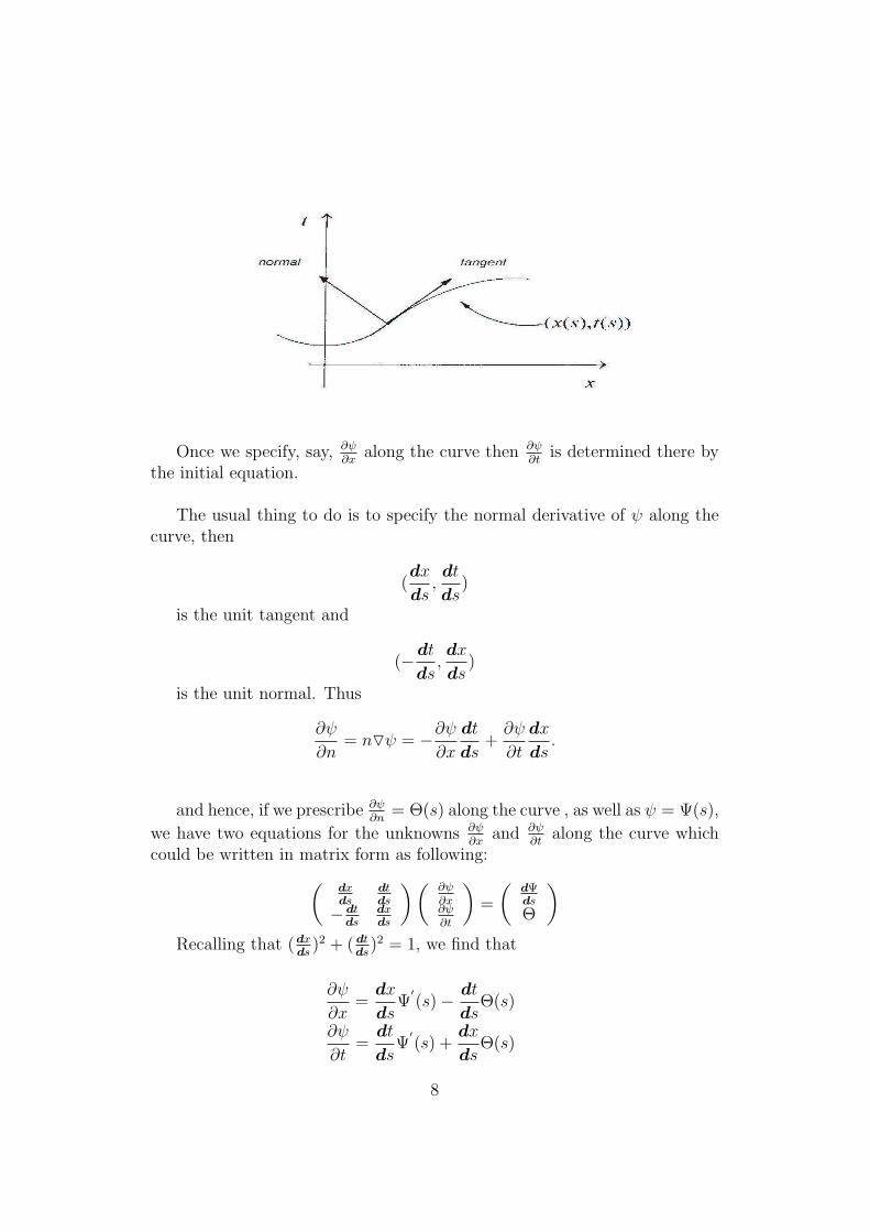
By the following classification method we can decide what sort of datashould be applied to a given PDE in order to get a well-posed problem. Forsimplicity we do this only for the case of a PDE in two variables, x and t(classification could be generalized for the case of n variables).
Consider the (possibly nonlinear) PDE
a∂2ψ
∂x2+ b
∂2ψ
∂x∂t+ c
∂2ψ
∂t2= f(x, t, ψ,
∂ψ
∂x,∂ψ
∂t) (1)
Suppose we prescribe ψ, ∂ψ∂x
and ∂ψ∂t
along some curve in the (x, t)-plane(see Figure below) and suppose this curve is given in a parameterized formas (x(s), t(s)) where s denotes arc length along this curve. Let us specifyfunction ψ along the curve, i.e.
ψ(x(s), t(s)) = Ψ(s),
then we have also implicitly specified the tangential derivative of Ψ alongthis curve, since, differentiating with respect to s we find
d
dsψ(x(s), t(s)) =
∂ψ
∂x
dx
ds+
∂ψ
∂t
dt
ds= Ψ
′(s)
Now notice that vector (dxds
, dtds
) is the unit vector tangent to the curve(x(s), t(s)) and hence
∂ψ
∂x
dx
ds+
∂ψ
∂t
dt
ds= L(s)Oψ =
∂ψ
∂L.
That is, the tangential derivative of ψ along the curve s is already knownif the value of ψ is known along the curve.
7
Once we specify, say, ∂ψ∂x
along the curve then ∂ψ∂t
is determined there bythe initial equation.
The usual thing to do is to specify the normal derivative of ψ along thecurve, then
(dx
ds,dt
ds)
is the unit tangent and
(−dt
ds,dx
ds)
is the unit normal. Thus
∂ψ
∂n= nOψ = −∂ψ
∂x
dt
ds+
∂ψ
∂t
dx
ds.
and hence, if we prescribe ∂ψ∂n
= Θ(s) along the curve , as well as ψ = Ψ(s),
we have two equations for the unknowns ∂ψ∂x
and ∂ψ∂t
along the curve whichcould be written in matrix form as following:
(dxds
dtds
− dtds
dxds
)(∂ψ∂x∂ψ∂t
)=
(dΨds
Θ
)
Recalling that (dxds
)2 + ( dtds
)2 = 1, we find that
∂ψ
∂x=
dx
dsΨ′(s)− dt
dsΘ(s)
∂ψ
∂t=
dt
dsΨ′(s) +
dx
dsΘ(s)
8

Thus, by prescribing ψ and ∂ψ∂n
along the curve (x(s), t(s)), we know all
of ψ, ∂ψ∂x
and ∂ψ∂t
along this curve. Now assume that a, b, c and f are functions
only of x, t, ψ, ∂ψ∂x
and ∂ψ∂t
, this means that all of these too are known along the
curve. That is, we have one equation for the three unknowns ∂2ψ∂x2 , ∂2ψ
∂x∂tand
∂2ψ∂t2
along the curve. But we can find two other equations by differentiatingexpressions for the first partial derivatives, namely
d
ds
∂ψ
∂x=
dx
ds
∂2ψ
∂x2+
dt
ds
∂2ψ
∂x∂t,
d
ds
∂ψ
∂t=
dx
ds
∂2ψ
∂x∂t+
dt
ds
∂2ψ
∂t2
This gives us the system of equations
dxds
dtds
00 dx
dsdtds
a b c
∂2ψ∂x2
∂2ψ∂x∂t∂2ψ∂t2
=
dds
(dxds
Ψ′ − dt
dsΘ)
dds
(dxds
Ψ′+ dt
dsΘ)
f
which provides solution if its determinant is non-zero:
dxds
dtds
00 dx
dsdtds
a b c
6= 0
i.e. if
a(dt
ds)2 − b
dx
ds
dt
ds+ c(
dx
ds)2 6= 0.
If however
a(dt
ds)2 − b
dx
ds
dt
ds+ c(
dx
ds)2 = 0,
then in general the system of equations above will be inconsistent and willhave no solutions. That means that the second partial derivatives can notexist along this curve and that means that PDE can not have a solution. Ifwe eliminate the parameter s, we may rewrite the condition of the existenceof solution in the form
dx
dt=
b
2a± 1
2a
√b2 − 4ac.
Any curve which satisfy these this condition is called characteristic curve orcharacteristic. Thus, Cauchy data, for instance, determine the solution of theproblem only if the curve is nowhere parallel to a characteristic. Obviously,there are three different cases to be regarded:
9

• b2 < 4ac, the characteristics are pure imaginary,
• b2 = 4ac, a single family of real characteristics,
• b2 > 4ac, a double family of real characteristics.
According to these conditions, all second order PDEs are divided intothree classes which are named elliptic, parabolic and hyperbolic by appealinganalogy with conical sections so that these names remind us about geometri-cal reasoning which led to this partition. To each class some specific bound-ary/initial conditions have to be prescribed in order to provide a well-posedproblem.
Class 1: b2 < 4ac, elliptic equations.
Examples:
• Laplace equation:52ψ = 0,
(note that operator 52ψ is commonly written as 4 in pure mathemat-ical texts),
• Helmholtz equation:52ψ + α2ψ = 0,
• Poisson’s equation:52ψ = −4πρ
Class 2: b2 = 4ac, parabolic equations.
Examples:
• heat conduction:
4ψ =1
α
∂ψ
∂t,
and the proportionality factor is called heat conductivity. The sameequation is used also for description of diffusion (with ψ as concentra-tion of the dissolved substance in the solvent and α - diffusivity) andalso is a form of the Navier-Stokes equation for a laminar fluid (withψ as internal friction of an incompressible fluid and α - kinematic vis-cosity).
10

• Schrodinger equation:
4ψ =2m
i~∂ψ
∂t,
which describes a vibration process (here m is mass of the particle, ~is Plank’s constant and i2 = −1).
Class 3: b2 > 4ac, hyperbolic equations.
Examples:
• wave equation:
4ψ =1
c2
∂2ψ
∂t2,
which is used in particular in acoustics (c is sound speed), electrody-namics of varying fields (c is light speed), in optics, in the theory ofwater waves, etc.
• four dimensional potential equation:
∑
k
∂2ψ
∂x2k
= 0,
which is used in special theory of relativity and is written out for threespace variables x1, x2, x3 and one time variable x4 = ict.
Now that we have specified three main classes of second order PDEs it ispossible to describe for each class what sort of boundary/initial conditionswill provide us a well-posed problem:
• parabolic - One initial (Cauchy)+ some boundary condition,
• elliptic - Dirichlet/Neumann/Robin,
• hyperbolic - One initial (Cauchy) + some boundary condition.
In this way we have specified a well-posed problem for a PDE of secondorder. But it does not mean that we are able to solve it! Even in case of firstorder the task of finding solutions is not solved completely. For some specifictypes of them the general solution is found, for instance, in case when x, t, ψare not included in the first order PDE explicitly, i.e. it has form
P (∂ψ
∂x,∂ψ
∂t) = 0,
11

then it has solutionψ = λ1x + λ2t + µ,
where P (λ1, λ2) = 0
or in case of generalized Clero equation
ψ = x∂ψ
∂x+ t
∂ψ
∂t+ f(
∂ψ
∂x,∂ψ
∂t)
with general solution
ψ = λx + µt + f(λ, µ).
As to general methods, methods of characteristics, Lax pair, Green func-tions, canonical transformations, etc. produce often solutions for some spe-cific PDE or groups of them. A great number of interesting results areobtained by the method of inverse scattering transform which allows to con-struct a PDE with given solution. In this way solutions of some famousPDEs have been obtained. Simply put, the inverse scattering transform is anonlinear analog of the Fourier transform used for linear problems. Its valuelies in the fact that it allows certain nonlinear problems to be treated by whatare essentially linear methods. For some important PDEs a lot of specificresults are obtained, for instance for PDE of only two variables x and t:
∂ψ
∂t+ 6ψ
∂ψ
∂x+
∂3ψ
∂x3= 0,
ψ(x, 0) = ψi(x),
ψ(0, t) = ψb(t),
with initial condition ψi(x) and boundary condition ψb(t). This equationis called linearized Korteweg-de Vries (KdV) equation and is generic equationfor the study of weak turbulence among long waves because it describes manyphysical phenomena such as plasma waves, Rossby waves, magma flow, sur-face water waves, etc. Hundreds of investigators dealt with this problem butno complete mathematical theory of this equation had yet been obtained.Of course, there are numerous number of results like, for instance, solitonsolutions on the infinite line, five different types of solution depending onthe relation between the initial and boundary values, solutions for positivequarter-plane problem (i.e. x > 0 and t > 0), solutions for negative quarter-plane problem (i.e. x < 0 and t > 0), solutions for time-dependent boundaryconditions, numerical solutions, etc.
12

Sometimes by simple transformation a nonlinear PDE could become lin-ear, for instance Thomas equation
ψxy + αψx + βψy + ψxψy = 0
could be made linear with a change of variables: ψ = logθ for some positivelydefined function θ:
ψx = (logθ)x =θx
θ, ψy = (logθ)y =
θy
θ,
ψxy = (θx
θ)y =
θxyθ − θyθx
θ2, ψxψy =
θxθy
θ2
and substituting this into Thomas equation we get finally linear PDE
θxy + αθx + βθy = 0.
General solution for particular case β = 0 can be obtained as a result of oneonce more change of variables: θ = φek1y which leads to
θx = φxek1y, θxy = φxye
k1y + k1φxek1y and φxy + (k1 + α)φx = 0,
and finally∂x(φy + (k1 + α)φ) = 0.
It givesφy − k2φ = f(y) with k2 = −(k1 + α)
and arbitrary function f(y). Now general solution can be obtained by themethod of variation of a constant. As a first step let us solve homogeneouspart of this equation, i.e. φy − k2φ = 0 and φ(x, y) = g(x)ek2y with arbitraryg(x). As a second step, suppose that g(x) is function on x, y, i.e. g(x, y),then initial equation takes form
(g(x, y)ek2y)y − k2g(x, y)ek2y = f(y),
g(x, y)yek2y + k2g(x, y)ek2y − k2g(x, y)ek2y = f(y),
g(x, y)yek2y = f(y), g(x, y) =
∫f(y)e−k2ydy + h(x),
and finally the general solution of Thomas equation with β = 0 can be writtenout as
φ(x, y) = g(x, y)ek2y = ek2y(
∫f(y)e−k2ydy + h(x)) = f(y) + ek2yh(x)
13

with two arbitrary functions f(y) and h(x). But generally speaking each newnonlinear PDE could turn out to be unsolvable!
Exercises:
1.1 Define the type and (if possible) class of following PDEs of two vari-ables x and t:
•ψtt − α2 52 ψ + β2ψ + ψψx = 0,
•ψtt − ψxx + ψ = 0,
•ψtt − α2 52 ψ − β2 52 ψtt + 3exJ2(ψ, t) = 0,
•ψt + αψx + βψxxx + ψψt + ψ2 = 0.
1.2 Prove that Burger’s equation
ψt + ψψx = αψxx
could be transformed to linear heat θt− θxx = 0 equation by substitution
ψ = −2(logθ)x.
How does this substitution change the class of the initial equation? Whyis it important?
1.3 Is Thomas’s equation quasi-linear?
1.4 Is Burger’s equation quasi-linear?
14
3 Dispersive waves
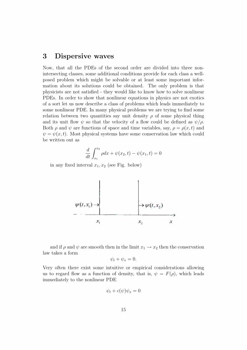
Now, that all the PDEs of the second order are divided into three non-intersecting classes, some additional conditions provide for each class a well-posed problem which might be solvable or at least some important infor-mation about its solutions could be obtained. The only problem is thatphysicists are not satisfied - they would like to know how to solve nonlinearPDEs. In order to show that nonlinear equations in physics are not exoticsof a sort let us now describe a class of problems which leads immediately tosome nonlinear PDE. In many physical problems we are trying to find somerelation between two quantities say unit density ρ of some physical thingand its unit flow ψ so that the velocity of a flow could be defined as ψ/ρ.Both ρ and ψ are functions of space and time variables, say, ρ = ρ(x, t) andψ = ψ(x, t). Most physical systems have some conservation law which couldbe written out as
d
dt
∫ x2
x1
ρdx + ψ(x2, t)− ψ(x1, t) = 0
in any fixed interval x1, x2 (see Fig. below)
and if ρ and ψ are smooth then in the limit x1 → x2 then the conservationlaw takes a form
ψt + ψx = 0.
Very often there exist some intuitive or empirical considerations allowingus to regard flow as a function of density, that is, ψ = F (ρ), which leadsimmediately to the nonlinear PDE
ψt + c(ψ)ψx = 0
15

with c(ψ) = Fx(ρ). This PDE describes a lot of different physical or tech-nical problems such as flood waves in rivers (wave’s height h plays the roleof density and c(h) is the flow velocity), transport flow (ρ now is number ofcars at the unit length of a highway, ψ is number of cars passing a line x inthe unit of time and highway has no outlets), erosion in mountains, chemicalexchange processes, absorption, etc.
It means that most of physical problems are described by nonlinear PDEswhich are very often of order more than 2 and mathematics provides no sys-tematic methods to solve them. Nevertheless, a very interesting way has beenfound by physicists in order to get some general information about physicallyimportant PDEs. In order to present here these results as a first step we re-strict ourselves in this section to linear PDEs.
Actually the main idea is very simple. If we are not able to classifyequations due to their form - let us try to classify them due to form of theirsolutions. The simplest possible solution whatsoever would be some nicesmooth periodical function like sine or cosine. Let us see, whether linearPDEs of arbitrary finite order which admit these type of solutions have alsosome other properties in common. Taking into account that the minimalnumber of variables in any PDE is equal two and without loose of generalitylet us regard following function of two variables:
ψ(x, t) = a sin(ωt− kx)
with
ω = 2πf =2π
T; k =
2π
λ;
where ω is wave frequency in radians and per second, f is wave frequency inHertz, k is wave number, T is wave period, λ is wave length. The constant ais called wave amplitude. The wave period is the time it takes two successivewave crests. The wave length λ is the distance two successive wave crests(see Fig. 1.1).
The basic feature of the wave as defined above is that the whole patternmoves along the x-axis as the time changes. Consider for simplicity the pointx = 0, t = 0, where ψ = 0. If now t starts to increase, the points x0(t) definedby x0(t)/λ = t/T will have the property that ψ(x0(t), t) = 0 for all t. Thepoint x0, where ψ = 0, thus moves with the velocity λ/T along the x-axis.
An additional angle α in the expression ψ = a sin(ωt−kx+α) is called aphase term. The whole argument of a sine is called a phase. Since sin(2πn+
16

α) = sin(2πn+α) for any n ∈ Z ∪0, phase difference of any multiple of 2πdo not matter at all. The phase of a point(x1, t1) will be equal to the phaseof the point (x2, t2) if
ωt1 + kx1 = ωt2 + kx2,
that is,
x2 − x1
t2 − t1=
ω
k=
λ
Tor
x2 = x1 +ω
k(t2 − t1).
Figure 1: A linear wave.
Thus point x2 on the x-axis which moves with velocity ω/k will have thesame phase for all times. Therefore, the velocity cph = ω/k = λ/T is calledphase velocity associated with the wave and this wave is called a travel-ling wave. Another important notion is a standing wave which does nottravel but remains in a constant position and occurs in nature whenever atravelling wave reflects perfectly from a boundary.
In this case reasoning similar to those concerning phase velocity lead tothe following definition of group velocity which indeed is generalization ofphase velocity for the case of travelling wave:
cgr =dω
dk,
17

Figure 2: The standing wave.
it is, so to say, ”phase velocity” of the wave’s envelope (see Figure below).
Difference between phase and group velocities is now obvious:
• Phase velocity cph = ω/k is velocity of points which belong to a onewave and have the same phase.
• Group velocity cgr = dω/dk is velocity of points which belong to agroup of waves and have the same amplitude.
Figure 3: The wave packet.
In general these two velocities do not coincide (see Exercises below) andgroup velocity plays more important role then phase velocity because it isthe velocity at which energy propagates.
18
Now notice that in physics it is usual to regard a wave in a form of complexexponent using Euler formula
exp ix = cos x + i sin x
because the operations like differentiation, multiplication, etc. become morecompact. Therefore from now on we will use also the complex representationfor a linear wave
ψ(x) = A exp i(kx− ωt)
keeping in mind that when necessary one takes the real part of it, namely
<(ψ(x)) = |A| cos(kx− ωt + α), α = argA.
Let us now write out explicitly a linear operator corresponding to 2-dimensionalPDE with constant coefficients in a form
P (∂
∂t,
∂
∂x),
where P is a polynomial which degree coincides with the order of PDE. Aftersubstituting a wave solution in it we will get
P (−iω, ik) = 0.
It means that in order to satisfy initial PDE wave number k and frequencyω have to be connected in some way, i.e. there exist some function f such,that
f(ω, k) = 0.
This connection is called dispersion relation. A solution of the dispersionrelation is called dispersion function, ω = ω(k). In general case, therecould be a few solutions, each of them is called mode of the dispersion func-tion. Since ω/k is phase velocity of a wave, ω is supposed to be a real-valuefunction. Another important point is that the very notion of dispersivewave systems (that is, dispersive PDE) has been introduced in order topoint out the difference between phase velocities of different waves providingsolutions of the same PDE. But the case of ω(k) = ck gives us the samephase velocity for all waves and therefore ideologically does not fall into theclass of dispersive waves. That is the reason why the following condition onthe ω has to be satisfied:
∂2ω
∂k26= 0
Actually this condition excludes also case of ω(k) = c1k + c2 due to somephysical reasons which we are not going to explain here (details see in [3],
19
[4]). The very important fact is that the initial PDE could be reconstructedby substituting −iω by ∂/∂t and ix by ∂/∂x.
Example
Let us regard a linear PDE
ψtt + α2φxxxx = 0.
and find explicit form of the dispersion function for it. First of all we needsome preliminary calculations:
ψt =∂
∂tψ = ω(−i)A exp i(kx− ωt),
ψtt =∂
∂t(∂
∂tψ) = (ω(−i))2A exp i(kx− ωt) = −ω2A exp i(kx− ωt),
ψx =∂
∂xψ = kiA exp i(kx− ωt),
........,
ψxxxx =∂4
∂x4ψ = (ki)4A exp i(kx− ωt) = k4A exp i(kx− ωt).
and substituting these results into initial PDE one gets:
0 = ψtt + α2ψxxxx =
= −ω2A exp i(kx− ωt) + α2k4A exp i(kx− ωt),
which leads to the dispersion function
ω(k) = ±αk2
with two modes: ω(k) = αk2 and ω(k) = −αk2.
All definitions and procedure above could be easily reformulated for acase of more space variables, namely x1, x2, ..., xn. In this case linear operatorgenerated by initial PDE takes form
P (∂
∂t,
∂
∂x1
, ...,∂
∂xn
),
and correspondingly dispersion function could be computed from
P (−iω, ik1, ..., ikn) = 0.
20

In this case we will have not a wave number k but a wave vector ~k =(k1, ..., kn) and the condition of non-zero second derivative of the dispersionfunction takes a matrix form:
| ∂2ω
∂ki∂kj
| 6= 0
Since ideally behavior of each physical system has to be described in time andspace, it is normal in physics to use different notations for these variables,for instance of a form
P (t, x1, ..., xn) = 0.
and the same in PDEs. In case when a PDE does not have variable t, it iscalled stationary PDE as, for instance, Laplace equation
∂2ψ
∂x2+
∂2ψ
∂y2+
∂2ψ
∂z2= 0.
In the opposite case PDE is called evolution PDE. The importance of thedifferent nature of these variables is recognized also in mathematics wherethe variables are called correspondingly time-like and space-like variables.Obviously the notion of dispersion is only important for evolution PDEs.
The division of the variables into these two classes originated from thespecial relativity theory where time and three-dimensional space are treatedtogether as a single four-dimensional manifold called space-time or Minkovskispace. In Minkovski space a metrics allowing to compute an interval s alonga curve between two events is defined analogously to distance in Euclideanspace:
ds2 = dx2 + dy2 + dz2 − c2dt2
where c is speed of light (sometimes the opposite choice of signs in the rightpart is chosen). However, note that whereas Euclidean distances are alwayspositive, Minkovski’s intervals may be positive, zero or negative. Events withspace-time interval zero are separated by the propagation of a light signal.Events with a positive space-time interval are in each other’s future or past,and the value of the interval defines the proper time measured by an observertravelling between them.
Note that in fact mathematical classification of PDEs into hyperbolic,parabolic or elliptic classes is not only too restrictive (strict definitions areonly possible for PDEs of second order) but also too abstract - it has no mem-ory whatsoever about the difference between space and time variables and all
21

the reasoning could be carried out for the case of any variables x1, x2, ..., xs.On the other hand, physical classification is based on the existence of twotypes of variables and it helps to construct physical interpretation of the so-lutions of PDE. What these two classifications have in common is followingworrying fact - both of them give us some ways to construct some solutionsof some PDEs in some special cases but not one of them provides either amethod to solve any specific PDE or at least a possibility to establish thatany specific PDE has a solution. Big advantage of physical classification isdue to the possibility to treat PDE of an arbitrary order.
Let us summarize the results obtained:
• We have constructed a one-to-one correspondence between linear (evo-lution) PDE L(ψ) = 0 of arbitrary order allowing a wave solution
ψ(~x) = A exp i(~k~x− ωt) and some polynomial P which defines disper-
sion function ω = ω(~k).
• The number of variables of dispersion function ω coincides with thenumber of space variables of the equation L(ψ) = 0.
• Given dispersion function allows us to re-construct the correspondinglinear PDE.
In this way the partitioning of all linear evolution PDEs into two classes- dispersive and non-dispersive - has been obtained.
This partition is not complementary to a standard mathematical one.
For instance, though hyperbolic PDEs normally do not have dispersivewave solutions, the hyperbolic equation ψtt − α2 52 ψ + β2ψ = 0 has them.Another case is the equation ψtt + α2φxxxx = 0 which could not be classifiedas hyperbolic, parabolic or elliptic but belongs to the class of dispersive PDEs.
Obviously in this way PDEs are able to generate only polynomial dis-persion relations. In fact, if some specific PDE is regarded together withspecial initial/boundary conditions, it may generate a transcendental disper-sion function such like
ω(k) = k tanh αk
and in general it is possible just to choose arbitrary dispersion function andto construct corresponding (perhaps integro-differential) equation in partialvariables.
22

Exercises:
2.1. Show that two waves sin(ωt − kx) and sin(ωt + kx) are moving inopposite directions.
2.2. Show that if ω and k are allowed to be negative and arbitrary phaseterms could be included, then all functions
a sin(kx− ωt),
a sin(kx + ωt +π
4),
a cos(ωt− kx) + b sin(ωt− kx)
may be written as a sin(ωt− kx + α) for appropriate choice of a, ω, k, α.
2.3. Compute dispersion relations for following PDEs of two variables xand t:
•ψtt − α2 52 ψ + β2ψ + ψψx = 0,
•ψtt − ψxx + ψ = 0,
•ψtt − α2 52 ψ − β2 52 ψtt + 3exJ2(ψ, t) = 0,
•ψt + αψx + βψxxx + ψψt + ψ = 0.
2.4. The same in case of three space variables, i.e. ~x = (x1, x2, x3).
2.5. Compute phase and group velocities for each PDE from 2.3.
23

4 Wave resonances
and perturbation techniques
Now that we know what a linear dispersive wave is, we are going to introducethe notion of the wave resonance which is the mile-stone for the whole theoryof nonlinear dispersive waves, that is for the theory of nonlinear dispersivePDEs. We begin with a well-known example illustrating the general idea ofthe resonance in some oscillating system.
Let us consider a linear oscillator driven by a small force
xtt + p2x = εeiΩt.
Here p is eigenfrequency of the system, Ω is frequency of the driving forceand ε > 0 is a small parameter. Deviation of this system from equilibriumis small (of order ε), if there is no resonance between the frequency of thedriving force εeiΩt and an eigenfrequency of the system. If these frequenciescoincide then the amplitude of resonator grows linearly with the time andthis situation is called resonance in physics. Mathematically it means ex-istence of unbounded solutions.
Let us now regard a (weakly) nonlinear PDE of the form
L(ψ) = εN(ψ)
where L is an arbitrary linear dispersive operator and N is an arbitrarynonlinear operator of second order which makes the formulae below moresimple. Two linear waves providing solutions of L(ψ) = 0 could be writtenout as
A1 exp i[~k1~x− ω(~k1)t],
A2 exp i[~k2~x− ω(~k2)t],
and their amplitudes A1, A2 are constant. Intuitively natural to expect thatsolutions of weakly nonlinear PDE will have the same form as linear wavesbut perhaps with amplitudes depending on time. Taking into account thatnonlinearity is small, each amplitude is regarded as a slow-varying functionof time, that is Aj = Aj(t/ε). Standard notation is Aj = Aj(T ) whereT = t/ε is called slow time.
Since wave energy is by definition proportional to amplitude’s square A2j
it means that in case of nonlinear PDE waves exchange their energy. This
24

effect can also be described as ”waves are interacting with each other” or”there exists energy transfer through the wave spectrum” or similar. Unlikelinear waves for which their linear combination was also solution of L(ψ) = 0,it is not the case for nonlinear waves!
Substitution of two linear waves into the operator εN(ψ) generates termslike
exp i[(~k1 ± ~k2)~x− [ω(~k1)± ω(~k2)]t
which play the role of a small driving force for the linear wave system (sameas in case of linear oscillator above). This driving force gives a small effect ona wave system till resonance occurs. i.e. till the wave number and the wavefrequency of the driving force does not coincide with some wave number andsome frequency of eigen-wave:
ω(~k1)± ω(~k2)± ω(~k3) = 0,
~k1 ± ~k2 ± ~k3 = 0.
This system is called resonance conditions and it describes resonancecurves or resonance surfaces depending on the number of space variables.Second equation is written out in vector form, that is we have one linearresonance condition if dim(~k) = 1 and few linear conditions if 1 ≤ dim(~k).In fact, it is not one system but a few different systems according to dif-ferent nontrivial choices of signs ”+” and ”-”. Each specific combinationgenerates a system to be solved and therefore resonance conditions describenot one but a few different algebraic systems. The dispersion ω is knownalgebraic function of space variables and its specific form could be computedfrom L(ψ) = 0. Therefore resonant conditions represent an algebraic system(strictly speaking, we would have to say a system of algebraic systems butfor brevity we will use words ”algebraic system” for resonance conditions.)
The number of unknowns is equal to the number of space variables.
The number of equations depends on the number of space variables andon the number of possible nontrivial combinations of signs ”+” and ”-” in it.
The solutions of this algebraic system(s), if any, provide coordinates ofwave vectors of three resonantly interacting waves
25

A1(T ) exp i[~k1~x− ω(~k1)t],
A2(T ) exp i[~k2~x− ω(~k2)t],
A3(T ) exp i[~k3~x− ω(~k3)t],
and one can see immediately that one main purpose - to find solutionsof the initial PDE - is not solved yet. We have found all ~ki but functionsA1(T ), A2(T ), A3(T ) are also to be found. These could be done by one ofthe perturbation methods (they are also called asymptotic methods) whichare much in use in physics and are dealing with equations having some smallparameter ε > 0 (see [6]). The main idea of such a method is very simple - anunknown solution, depending on ε, is written out in a form of infinite serieson different powers of ε and coefficients before any power of ε are computedconsequently.
In order to demonstrate how it works let us take a simple algebraic equa-tion
x2 − (3− 2ε)x + 2 + ε = 0
and try to find its asymptotic solutions. In case ε = 0 we get
x2 − 3x + 2 = 0
with roots x = 1 and x = 2. The first equation is called perturbed and thesecond - unperturbed. Natural suggestion is that the solutions of perturbedequation differ only a little bit from the solutions of unperturbed one.
First step. Look for the perturbed solutions in a form
x = x0 + εx1 + ε2x2 + ...
with x0 as a solution of unperturbed equation which in our case means x0 = 1or x0 = 2.
Second step. Substitute this infinite series into the given equation andrewrite it in such a way that all the terms with same degree of ε are collectedtogether. In our case it leads to
ε0 : x20 − 3x0 + 2,
ε1 : 2x0x1 − 3x1 − 2x0 + 1,
ε2 : 2x0x2 + x21 − 3x2 − 2x1,
...
26

Third step. Suppose that all coefficients corresponding to the consequentpowers of ε are zero and solve the system (notice that first equation here isunperturbed initial equation whose solutions are already known):
x20 − 3x0 + 2 = 0,
2x0x1 − 3x1 − 2x0 + 1 = 0,
2x0x2 + x21 − 3x2 − 2x1 = 0,
...
Then the resulting solutions of perturbed equation are
x0 = 1, x1 = −1, x2 = 3, ...
x = 1− ε + 3ε2 + ...
and
x0 = 2, x1 = 3, x2 = −3, ...
x = 2 + 3ε− 3ε2 + ...
Now we see that perturbation technique generates a system of equationswhich being solved consequently gives us the coefficients in front of any de-sirable degree of ε in the general solution of the perturbed equation. Equationabove was chosen as example because it’s exact solutions are known and onewould be able to compare them with the results obtained by perturbationmethod. Indeed, exact solutions of perturbed equation are
x =1
2[3 + 2ε±
√1 + 8ε + 4ε2]
and substituting binomial representation for the expression under the squareroot
(1 + 8ε + 4ε2)12 = 1 + (8 + 4ε2) +
12(−1
2)
2!(8ε + 4ε2)2 + ... =
= 1 + 4ε + 2ε2 − 1
8(64ε2 + ...) =
= 1 + 4ε− 6ε2 + ...
into the exact solution one gets finally
x =1
2(3 + 2ε− 1− 4ε + 6ε2 + ...) =
= 1− ε + 3ε2 + ...
x =1
2(3 + 2ε + 1 + 4ε− 6ε2 + ...) =
= 2 + 3ε− 3ε2 + ...
27

as before.
This check gives mathematician a feeling that ”there is something inperturbation methods” but not much more - no strict mathematical proof ofthem being always correct and/or providing always good approximate (physi-cists call them asymptotic) solutions or something of this kind. On the otherhand, perturbation methods are very successfully used in physics and engi-neering for the problems having no known exact solutions.
We demonstrate below how to use perturbation method for barotropicvorticity equation (BVE) is also known as Obukhov-Charney or Hasegawa-Mima equation. The number of names given to it is explained by its im-portance in many physical applications - from geophysics to astrophysics toplasma physics: the equation was again and again re-discovered by special-ists in very different branches of physics. In particular, taken in sphericalform it describes planetary (or Rossby) waves in an ocean or in the Earthatmosphere which appear due to the rotation of the Earth.
Being regarded on a sphere, BVE takes following form
∂4ψ
∂t+ 2
∂ψ
∂λ+ εJ(ψ,4ψ) = 0. (2)
Here ψ is the stream-function; variables t, φ and λ physically mean thetime, the latitude (−π/2 ≤ φ ≤ π/2) and the longitude (0 ≤ λ ≤ 2π) respec-tively; 0 < ε << 1 is small parameter. The spherical Laplacian and Jacobianare given by formulae
4ψ =∂2ψ
∂φ2+
1
cos2 φ
∂2ψ
∂λ2− tan φ
∂ψ
∂φ
and
J(a, b) =1
cosφ(∂a
∂λ
∂b
∂φ− ∂a
∂φ
∂b
∂λ)
respectively. The linear part of spherical BVE has wave solutions in theform
APmn (µ) exp i[mλ +
2m
n(n + 1)t],
28

where ~k = (m,n), µ = sin φ, ω = −2m/[n(n + 1)], Pmn (x) is the as-
sociated Legendre function of degree n and order m and A is constant waveamplitude.
In this place mathematician gets a shock - till now linear wave was sup-posed to have much more simple form, namely, A exp i[~k~x− ω(~k)t] withoutany additional multiplier of a functional form. A physicist says that it isintuitively clear that if multiplier is some oscillatory function of only spacevariables then we will still have a wave of a sort ”but it would be difficultto include it in an overall definition. We seem to be left at present with thelooser idea that whenever oscillations in space are coupled with oscillation intime through a dispersion relation, we expect the typical effects of dispersivewaves” [3]. By the way, most physically important dispersive equations havethis form of waves.
Now let us keep in mind that a wave is something more complicated thenjust a cosine but still smooth and periodical let us look where perturbationmethod will lead us. An approximate solution has a form
ψ = ψ0(λ, φ, t, T ) + εψ1(λ, φ, t, T ) + ε2ψ2(λ, φ, t, T ) + ...
where T = t/ε is the ”slow” time and the zero approximation ψ0 is givenas a sum of three linear waves:
ψ0(λ, φ, t, T ) =3∑
k=1
Ak(T )P (k) exp(mkλ− ωkt)
with notations P (k) = Pmknk
and ωk = ω(mk, nk). Then
ε0 :∂4ψ0
∂t+ 2
∂ψ0
∂λ= 0,
ε1 :∂4ψ1
∂t+ 2
∂ψ1
∂λ= −J(ψ0,4ψ0)− ∂4ψ0
∂T,
ε2 : .....
To calculate the right part of last equation some preliminary calculationsare necessary (notation θk = exp(mkλ− ωkt)):
29

∂ψ0
∂λ= i
3∑
k=1
P (k)mk[Ak exp(iθk)− A∗k exp(−iθk)];
∂2ψ0
∂λ2= −
3∑
k=1
P (k)m2k[Ak exp(iθk) + A∗
k exp(−iθk)];
∂ψ0
∂φ=
3∑
k=1
d
dφP (k) cos φ[Ak exp(iθk) + A∗
k exp(−iθk)];
∂2ψ0
∂φ2=
3∑
k=1
[d2
dφ2P (k) cos2 φ− d
dφP (k) sin φ][Ak exp(iθk) + A∗
k exp(−iθk)];
4ψ0 = −3∑
k=1
P (k)Nk[Ak exp(iθk) + A∗k exp(−iθk)];
(where notation Nk = nk(nk + 1) and the definition of Legendre functionas a solution of the following equation:
(1− z2)d2P
dz2− 2z
dP
dz+ [n(n + 1)− m2
1− z2]P = 0
has been used in order to obtain the last equation);
∂4ψ0
∂λ= i
3∑
k=1
P (k)mkNk[Ak exp(iθk)− A∗k exp(−iθk)];
∂4ψ0
∂φ= −
3∑
k=1
Nkd
dφP (k) cos φ[Ak exp(iθk) + A∗
k exp(−iθk)];
J(ψ0,4ψ0) =
−i
3∑
j,k=1
NkmjP(j) d
dφP (k)[Aj exp(iθj)− A∗
j exp(−iθj)][Ak exp(iθk) + A∗k exp(−iθk)] +
+i
3∑
j,k=1
NkmkP(k) d
dφP (j)[Aj exp(iθj) + A∗
j exp(−iθj)][Ak exp(iθk)− A∗k exp(−iθk)];
∂4ψ0
∂T=
3∑
k=1
P (k)Nk[dAk
dTexp(iθk) +
dA∗k
dTexp(−iθk)].
The condition of unbounded growth of the left hand can be written outin the form
30

J(ψ0,4ψ0) =∂4ψ0
∂T
and therefore the resonance conditions take form of
θj + θk = θi ∀j, k, i = 1, 2, 3.
Let us fix some specific resonance condition, say,
θ1 + θ2 = θ3,
which means
ω1 + ω2 = ω3, & m1 + m2 = m3, (3)
then
∂4ψ0
∂T∼= −N3P
(3)[dA3
dTexp(iθ3) +
dA∗3
dTexp(−iθ3)],
J(ψ0,4ψ0) ∼= −i(N1 −N2)(m2P(2) d
dφP (1))−m1P (1)
d
dφP (2) ·
A1A2 exp[i(θ1 + θ2)]− A∗1A
∗2 exp[−i(θ1 + θ2)],
where notation ∼= means that only terms which can generate given reso-nance are written out. Let us substitute these expressions into the coefficientby ε1, i.e. into the equation
∂4ψ1
∂t+ 2
∂ψ1
∂λ= −J(ψ0,4ψ0)− ∂4ψ0
∂T,
multiply both parts of it by
P (3) sin φ[A3 exp(iθ3) + A∗3 exp(−iθ3)]
and integrate all over the sphere with t → ∞. As a result two followingequations can be obtained:
N3dA3
dT= 2iZ(N2 −N1)A1A2,
N3dA∗
3
dT= −2iZ(N2 −N1)A
∗1A
∗2,
where
31

Z =
∫ π/2
−π/2
[m2P(2) d
dφP (1) −m1P
(1) d
dφP (2)]
d
dφP (3)dφ.
The same procedure obviously provides the analogous equations for A2
and A3 while fixing corresponding resonance conditions:
N1dA1
dT= −2iZ(N2 −N3)A3A
∗2,
N1dA∗
1
dT= 2iZ(N2 −N3)A
∗3A
∗2,
N2dA2
dT= −2iZ(N3 −N1)A
∗1A3,
N2dA∗
2
dT= 2iZ(N3 −N1)A1A
∗3.
This system of 6 ODEs on Ai, A∗i is normally written in the form
N1A1 = Z(N2 −N3)A2A3,
N2A2 = Z(N3 −N1)A1A3,
N3A3 = Z(N1 −N2)A1A2,
(4)
for real-valued amplitudes A1, A2, A3 meaning that two analogous sys-tems of ODEs have to be solved - one for real parts of amplitudes and onefor their imaginary parts.
Obviously only the case when Z 6= 0 has to be regraded while otherwiseAi = 0 and it is linear case. It could be shown that Z 6= 0 if the followingconditions keep true:
|n1 − n2| ≤ n3 ≤ n1 + n2,
n1 + n2 + n3 is odd,
mi ≤ ni ∀i = 1, 2, 3,
Coefficient of Z is called interaction coefficient and plays important physicalrole - it characterizes the velocity of energy exchange between the waves ofthe triad. Explicit form of the interaction coefficients depends on the formof dispersion function (that is, on the form of initial PDE) and coordinatesof wave vectors. Interaction coefficients must not be identically equal tozero (otherwise amplitudes would not be changing and one would be backin linear case). Therefore some additional restrictions are sometimes added
32

to the general resonance conditions, namely in our case resonant conditionstake form:
ω1 + ω2 = ω3,
m1 + m2 = m3,
mi ≤ ni ∀i = 1, 2, 3,
|n1 − n2| ≤ n3 ≤ n1 + n2,
n1 + n2 + n3 is odd,
ni 6= nj ∀i 6= j.
(5)
Notice that Sys.(4) can be solved explicitly in terms of Jacobian ellipticfunctions [5]. Here we are not going into the full details of its derivationbut just give the main idea. First of all, we note that the system has twoconserved integrals. The first one is called energy conservation law and couldbe obtained by multiplying the i-th equation by Ai, i = 1, 2, 3 and adding allthree of them:
N1A21 + N2A
22 + N3A
23 = c1.
The second conserved integral is called enstrophy conservation law and isobtained by multiplying the i -th equation by NiAi, i = 1, 2, 3 and adding allthree of them:
N21 A2
1 + N22 A2
2 + N23 A2
3 = c2.
The constants c1 and c2 depend, of course, on the initial values of Ai0, i =1, 2, 3. Using these two conservation laws one can easily obtain expressionsfor A2 and A3 in terms of A1. Substitution of these expressions into the firstequation of our ODE system gives us differential equation of the first orderwhich explicit solution is one of Jacobian elliptic functions. In similar waywe will get expressions for the amplitudes A2 and A3 as well, so that thegeneral solution has form:
A1 = b1cn(t/t0 − λ),
A2 = b2dn(t/t0 − λ),
A3 = b3sn(t/t0 − λ),
where
b21 = A2
10 + N3(N2 −N3)/N1(N2 −N1)A230,
b22 = A2
20 + N3(N3 −N1)/N2(N2 −N1)A230,
b23 = A2
30 + N1(N2 −N1)/N3(N2 −N3)A210,
33

the constant t0 depends on wave numbers and initial values of amplitudesas follows:
t0 =1
Z[N2 −N3
N1
(N3 −N1
N2
A230 +
N2 −N1
N3
A220)]
1/2
and the constant λ is obtained from the initial conditions.
The Jacobian elliptic functions cn, sn, dn can be defined in the followingway. Let
u =
∫ φ
0
dθ
(1− µ sin2 θ)1/2
and let define three following functions:
snu = sin φ,
cnu = cos φ,
dnu = (1− µ sin2 φ)1/2.
These functions are periodic in u. The periods of snu and cnu are equalto 4K and the periods of dnu is equal to 2K where
K =
∫ π/2
0
dθ
(1− µsin2θ)1/2
is complete elliptic integral and
µ =A2
10N1
N3−N2+ A2
20N2
N3−N1
A230
N3
N2−N1+ A2
20N2
N3−N1
is modulus of the elliptic functions. The period of energy exchange withinthe modes of a resonant triad could be calculated as
τ = 4pt0K, p = 1, 2, 3, ...
Summing up, we described in all details the energetic behavior of threearbitrary resonantly interacting waves. As a result system of ODEs for slowlychanging waves amplitudes is obtained
A1 = C1A2A3,
A2 = C2A1A3,
A3 = C3A1A2,
34

where Ai are functions of one variable T and of a few parameters which arethe wave numbers giving solutions of resonance conditions (three parameters
for the case dim(~k) = 1, six parameters for the case dim(~k) = 2 and so on).The only difference with the results obtained for perturbed polynomial is thefollowing: perturbation technique applied for a polynomial generates systemof polynomials to be solved while applied for PDE it generates a system ofODEs.
The only problem left is that the space of wave numbers is infinite andit means that in fact we have to solve a much more complicated system ofODEs, namely
A1 = C1,3A2A3 + C1,4A2A4 + ... + C1,sA2As + ...,
A2 = C2,3A1A3 + C2,4A1A4 + ... + C2,sA1As + ...,
.....
for the case of quadratic nonlinearity. This system connects all existing wavesand they are infinitely many which makes it difficult to solve these ODEs,whether analytically or numerically. What are the possibilities we will see inthe next Section.
5 Classification of dispersive PDEs
Let us notice fist that all the considerations above could be carried out forthe nonlinearity of arbitrary order n in which case resonance conditions
ω(~k1)± ω(~k2)± ...± ω(~kn+1) = 0,~k1 ± ~k2 ± ...± ~kn+1 = 0.
(6)
describe (n + 1)-wave interactions so that cubic nonlinearity generatesfour-wave interactions, nonlinearity of fourth order generates five-wave inter-actions and so on. Corresponding system of ODEs on the slowly-changingamplitudes will have terms like A1A2...An+1 on the right hand:
A1 = C1A2A3A4...An+1 + ...,
A2 = C2A1A3A4...An+1 + ...,
...
An+1 = CrA1A2A3...An + ...,
...
(7)
35

Let us sum up what we got till now:
Beginning with PDE L(ψ) = εN(ψ) some algebraic system (resonanceconditions) and some system of ODEs have been constructed. When solvedtogether they may provide solution(s) of the initial PDE.
To solve this system of ODEs a special methodof wave kinetic equation has been developed in 60-th (see, for instance,[14], [10] ) and applied for many different types evolution PDEs. Kineticequation is approximately equivalent to the initial nonlinear PDE but hasmore simple form allowing direct numerical computations of each wave am-plitudes in a given domain of wave spectrum. Wave kinetic equation is anaveraged equation imposed on a certain set of correlation functions and itis in fact one limiting case of the quantum Bose-Einstein equation while theBoltzman kinetic equation is its other limit. Some statistical assumptionshave been used in order to obtain kinetic equations and limit of its applica-bility then is a very complicated problem which should be solved separatelyfor each specific equation [13].
Simply formulated, conditions used for obtaining of kinetic equation canbe described as following:
• each wave takes part in resonant interactions,
• each wave interacts with all other waves simultaneously,
• all wave amplitudes are of the same order.
As a result, the Sys.(7) has been reduced to an equation of a form
d
dTAi =
∫G(~ki)δ(
∑~ki)d~ki
which is solved in respect to each separate wave amplitude Ai. Here functionG depends on the form of initial nonlinear PDE and notation δ(
∑~ki) is usedfor delta-function which is equal to zero on the solutions of Sys.(6).1) and isnon-zero otherwise. Wave kinetic equation is often written out in the form
d
dTA2
i =
∫G(~ki)δ(
∑~ki)d~ki
because amplitude square is proportional to the wave energy and this formallows to treat the results produced by kinetic equation in terms of energy
36

exchange between the interacting waves.
Thus, the existence of resonances, i.e. solutions of Sys.(6), in a (n + 1)-wave system for some specific PDE allows physicist to replace the PDE bykinetic equation which govern energy transfer through the spectrum. A veryinteresting fact is that even some classification of dispersive PDEs due totheir integrability properties was constructed basing on solutions of Sys.(6).We present it below very briefly and for more details see [7].
First of all, it was proven that in case when Eq.(6.1) does not have anysolutions, initial nonlinear PDE could be transformed into a linear PDEby canonic transformation. If, on the other hand, Eq.(6.1) does have somesolutions, then initial PDE will still have some nonlinearity after canonictransformation and it could be written out as
ΣiTiδ(~k1 ± ~k2 ± ...± ~ki)
ω(~k1)± ω(~k2)± ...± ω(~ki)
where δ is a delta-function and so-called here vertex coefficient Ti and infact Ti0 for some specific i0 is just some generalization of interaction coef-ficient from the system for slowly changing amplitudes in case of i0-wavesinteractions. In case of zero vertex coefficient, Ti = 0 we fall into the class ofequations having soliton solutions and in case of non-zero vertex coefficients,as it was shown before, the kinetic equation is constructed which is, to someextent, equivalent to the initial PDE. The words ”to some extent” are herein order to remind us that some additional physically natural assumptionswere used in order to construct kinetic equation.
Now it looks like all dispersive PDEs are classified and the work of physi-cist is finished while the only task left to mathematician is to prove conver-gence of perturbation methods. But it’s not true! Kinetic equations havebeen written for infinite interaction domains, i.e. for an infinite plane or aninfinite channel and were used successfully for about 25 years for descrip-tion of many types of waves, mostly in cases for 3- and 4-waves interactions.The results of laboratory experiments showed that ”reasonable agreementis normally obtained with theoretical results for the infinite case” [8], if thewavelength are small enough in comparison to the size of the experimentalbasin. The cases when wavelengths are comparable with the characteristicsizes of the experimental basin remain, as a rule, unexplained [9] and havebeen named ”effects of finite lengths” [8]. Attempts to put some additional
37
”physically relevant” terms into the kinetic equations in order to make themapplicable to long-wavelength systems have failed. The author of the pio-neering work in this field, O. Phillips, who obtained the first kinetic equationin [10] wrote in [11] that ”new physics, new mathematics and new intuitionis required” in order to understand energetic behavior of long-wavelengthsystems (they are also called large-scale systems).
From physical point of view large-scale wave system is a system wherewave do notice the boundaries. Mathematically it means that initial PDEhas to be regarded with zero or periodical boundary conditions. These wavesystems are called resonators and are very important in numerous number ofphysical applications [12]. From mathematical point of view, difference be-tween infinite interaction domain and resonator could formulated very easily:
• In case of infinite interaction domain Sys.(6) have to be solved in realnumbers.
• In resonators Sys.(6) have to be solved in integers.
It means that in resonators Sys.(6) describe a system of Diophantine oralgebraic equations in integers. When a specialist in number theory or inalgebra looks at assumptions used for obtaining of kinetic equations togetherwith discrete Sys.(6), he starts to worry. Why do any pair of integers (m,n)has to be part of some solution? Or, even more, to be part of infinitely manysolutions? Is it really true that this algebraic system always has infinitelymany solutions? Rather not. At least, one has to prove it.
In the next Part, Part 2: Properties of discrete resonant systems,it will be proven that all these physical assumptions do not hold in resonators,and this is the reason why method of kinetic equation does not work there.It means that this class of wave systems can not be described in terms of ki-netic equation principally and has to be studied separately. In Figure belowwe show where this ”missing term” in the classification of dispersive PDEshas to be inserted.
In Part 2 a new approach will be presented to study discrete resonancesystems based mainly on number theory methods. Some general properties ofthese systems are described analytically and corresponding results for manyspecific physical problems examples are presented.
38

39

References
[1] V.E. Zakharov. How classical physics helps mathematics, In book: Vi-sions in Mathematics: Towards 2000, Part II. Eds.: N. Alon, J. Bour-gain, A. Connes, M. Gromov, V. Milman, pp. 859-881. Birkhauser Verlag(2000)
[2] V.I. Arnold. Lectures on Partial Differential Equations. SpringerSeries: Universitext, 2004, 157 pages, ISBN: 3-540-40448-1
The text is written for highly educated mathematicians, illustrated witha lot of geometrical figures and covers basic parts on the theory oflinear PDEs. General concepts of the Hamiltonian formalism, integralmanifolds, differential geometry are supposed to be known.
[3] G. B. Whitham. Linear and Nonlinear Waves. Wiley Series in Pureand Applied Mathematics, 1999, 636 pages, ISBN: 0-471-35942-4
Classical volume on hyperbolic and dispersive waves. Different generalmathematical aspect and special cases are discussed and illustrated withnumerous number of physical and technical examples, beginning with thevery definition of dispersive waves. Probably the best book on the subject!
[4] G. B. Whitham. Lectures on wave propagation. Springer for TATAINSTITUTE OF FUNDAMENTAL RESEARCH, Bombay, 1979, 148pages, ISBN: 0-387-08945-4
Simply written, a lot of examples, stimulates appearance of physicalintuition by a reader. Many our examples are taken from these two books.
[5] Whittaker E.T. A treatise on the analytical dynamics of particlesand rigid bodies. Cambrige Univercity Press, Cambrige, 1937
[6] Nayfeh A.N. Introduction to perturbation techniques. Wiley-Interscience, NY, 1981
Similarities, differences, advantages and limitations of different pertur-bation methods are pointed out concisely. The techniques are described by
40

means of many examples of algebraic and ordinary differential equations.
[7] Shulman E., Zakharov V. In book: (Ed.) V.E.Zakharov, What isIntegrability? Springer, Berlin, (1991)
[8] Craik A.D.D. Wave Interactions and Fluid Flows. Cambridge:Cambridge University Press, p.249 (1985)
[9] Hammack J.L., Henderson D.M. ”Resonant interactions among surfacewater waves”. Ann. Rev. Fluid Mech. 25: 55-96 (1993)
[10] Phillips O. ”On the dynamics of unsteady gravity waves of infiniteamplitude” J. Fluid Mech, 9, p.193-217 (1960)
[11] Phillips O. ”WAve interactions - evolution of an idea” J. Fluid Mech,106, pp.215-27 (1981)
[12] Rabinovich M., Trubetskov D. Oscillations and Waves in Linearand Nonlnear Systems. Kluver Academic Publishers, Dordrecht.Soviet Series, Vol. 50 (1989)
[13] Zakharov V. ”Statistical theory of gravity and capillary waves on thesurface of a finite-depth fluid.” Eur. J. Mech. B: Fluids, pp.327-344(1999)
[14] Hasselman K. ”On nonlinear energy transfer in gravity-wave spectrum.Part 1. General theory.” J. Fluid Mech., V.12, pp.481-500 (1962)
41