dinural variation of terrestrial magnetism
TRANSCRIPT
7/27/2019 Dinural Variation of Terrestrial Magnetism
http://slidepdf.com/reader/full/dinural-variation-of-terrestrial-magnetism 1/42
L163 ]
IV^. The Diurnal Variation of Terrestrial Magnetism.
By Arthur Schuster, F.R.S,
Received October 31,—liead November 7, 1907.
1. In a previous communication'^ I proved that the Diurnal Variation of Terrestrial
Magnetism has its origin outside the earth's surface and drew the natural conclusion
that it was caused by electric currents circulating in the upper regions of the
atmosphere. If we endeavour to carry the investigation a step further and enquire
into the probable origin of these currents, we have at present no alternative to the
theory first proposed by Balfour Stewart that the necessary electromotive forces
are supplied by the permanent forces of terrestrial magnetism acting on the bodily
motion of masses of conducting air which cut through its lines of force. In the
language of modern electrodynamics the periodic magnetic disturbance is due to
Foucault currents induced in an oscillating atmosphere by the vertical magnetic
force. The problem to be solved in the first instance is the specification of the
internal motion of a conducting shell of air, which shall, under the action of given
magnetic forces, determine the electric currents producing known electromagnetic
effects. Treating the diurnal and semidiurnal variations separately, the calculation
leads to the interesting results that each of them is caused by an oscillation of the
atmosphere which is of the same nature as that which causes the diurnal changes of
barometric pressure. The phases of the barometric and magnetic oscillations agree
to about If hours, and it is doubtful whether this difference may not be due to
uncertainties in the experimental data. In the previous communication referred to
I already tentatively suggested a connexion between the barometric and magnetic
changes, but it is only recently that I have examined the matter more closely. In
the investigation which follows I begin by considering the possibility that both
variations are due to one and the same general oscillation of the atmosphere. The
problem is then absolutely determined if the barometric change is known, and we
may calculate within certain limits the conducting power of the air which is sufficient
and necessary to produce the observed magnetic effects ; this conducting power is
found to be considerable. It is to be observed, however, that the electric currents
producing the magnetic variations circulate only in the upper layers of the
atmosphere, where the pressure is too small to affect the barometer ; the two
* 'Phil. Trans.,' A, vol. 180, p. 467 (1889).
VOL. CCVIII.—A 430. y 2 22,4.08

7/27/2019 Dinural Variation of Terrestrial Magnetism
http://slidepdf.com/reader/full/dinural-variation-of-terrestrial-magnetism 2/42
164 MR AETHUR SCHUSTER ON THE
variations have their origin therefore in different layers, which may to some extent
oscillate independently. Though we shall find that the facts may be reconciled with
the simpler supposition of one united oscillation of the whole shell of air, there are
certain difficulties which are most easily explained by assuming possible differences
in phase and amplitude between the upper and lower layers. If the two oscillations
are quite independent, the conducting power depending on the now unknown
amplitude of the periodic motion cannot be calculated, but must still be large, unless
the amplitude reaches a higher order of magnitude than we have any reason to
assume.
The mathematical analysis is simple so long as we take the electric conductivity of
the air to be uniform and constant ; but the great ionisation which the theory
demands requires some explanation, and solar radiation suggests itself as a possible
cause. Hence we might expect an increased conducting power in summer and in
daytime as compared with that found during winter and at night. Observation shows,
indeed, that the amplitude of the magnetic variation is considerably greater in
summer than in winter, and we know that the needle is at comparative rest during
the night. The variable conducting power depending on the position of the sun helps
us also to overcome a difficulty which at first sight would appear to exclude the
possibility of any close connexion between the barometric and magnetic variations;
the difficulty is presented by the fact that the change in atmospheric pressure is
mainly semidiurnal, while the greater portion of the magnetic change is diurnal.
This may to some extent be explained by the mathematical calculation, which shows
that the flow of air giving a 24 -hourly variation of barometric pressure is more
effective in causing a magnetic variation than the corresponding 12-hourly variation,
but the whole difference cannot be accounted for in this manner. If, however, the
conductivity of air is greater during the day than during the night, it may be proved
that the 12-hourly variation of the barometer produces an appreciable periodicity of
24 hours in the magnetic change, while there is no sensible increase in the 12-hourly
magnetic change due to the 24-hourly period of the barometer. The com2Dlete
solution of the mathematical problem for the case of a conducting power proportional
to the cosine of the angle of incidence of the sun's rays is given in Part II. But even
this extension of the theory is insufficient to explain entirely the observed increased
amplitude of the magnetic variation during summer. We are, therefore, driven to
assume either that the atmospheric oscillation of the upper layer is greater in summer
than in winter and is to that extent independent of the oscillation of the lower layers,
or that the ionising power of solar radiation is in some degree accumulative and that
atmospheric conductivity is therefore not completely determined by the position of
the sun at the time. The increased amplitude at times when sunspots are frequent
is explained by an increased conductivity corresponding to an increase in solar
activity. All indications, therefore, point to the sun as the source of ionisation, and
ultra-violet radiation ^eems to be the most plausible cause. ,
7/27/2019 Dinural Variation of Terrestrial Magnetism
http://slidepdf.com/reader/full/dinural-variation-of-terrestrial-magnetism 3/42
DIUENAL VAEIATION OF TEEEESTEIAL MAGNETISM. 165
2. The velocity potential of a horizontal irrotational motion of the earth's
atmosphere considered as an infinitely thin shell is necessarily expressible as a series
of spherical harmonics from which V\^e may select for consideration the one of degree
n and type o", writing it xfj/ sin {cr {\+ t)— a} or i/// according to convenience. The
longitude X is measured from any selected meridian towards the east, while t is the
time of the standard meridian in angular measure. As in the greater part of the
investigation X and t occur in the combination X + t only, we may frequently omit t
without detriment to the clearness, noting, however, that if the differentiation with
respect to t is replaced by a differentiation with respect to X we must apply the factor
27r/N, where N is the number of seconds in the day.
I consider in the first instance the electric currents which are induced in air moving
horizontally under the infl.uence of the earth's vertical magnetic force. Assuming the
earth to be a uniformly magnetised sphere, its potential may be resolved into the
zonal harmonic of the first degree and the tesseral harmonic of the first type and
degree. The angle between the magnetic axis and the geographical axis not being
great, the zonal harmonic constitutes by far the largest part, and forms the first
subject of our investigation. As far as this part is concerned, we may put the vertical
force equal to C cos 0, where is the colatitude and C, measured upwards, has a
numerical value differing little from —f.
The components of electric force, X and Y, measured towards the south and east
respectively, are
Xa = Ccot^^, Ya = --Ccos^^ ...... (1),dk da '
and these equations may be written in the form
r?. . 71+ 1 . Xa = ^-ttXz + C -V—̂ -,--( 7^ . n+ 1 . i/; cos ^— sin Q -^
dddX smUdXX ddj
n.n+l.Ya^C^^,-G^^ (n .n+1 .r^ oos0-sin0^'
y (2).
y
where n is the degree of the harmonic.
The identity between (1) and (2) is obvious as regards the first of the equations,
and the reduction of the second is obtained with the help of the fundamental equation
sin^4sin^^ + ^+n.n+l.sin^^.t/. = 0,
d0 d0 d)\?
\\s being a zonal harmonic of degree n.
The components of electric force are by (2) reduced to the form
Y _ _ c^S (iR , Y _ _ <^S (JR /o\"~
ad0 a sin dk'
aBm0 dk ad0 ''
* * /'

7/27/2019 Dinural Variation of Terrestrial Magnetism
http://slidepdf.com/reader/full/dinural-variation-of-terrestrial-magnetism 4/42
166 ME. AETHUE SCHUSTEE ON THE
and may be divided into two portions, the first of which is derivable from a potential
S = -C#/».(,-Kl).
In the steady state this part is balanced by a static distribution of electricity
revolving round the earth and causing a variation in the electrostatic potential which
is found to be too weak to affect our instruments. The second portion of the electric
force produces electric currents ; these, neglecting electric inertia—which will be
considered later—have pR as current function, where p is the conductivity of the
medium.
The comparison of (2) and (3) shows that
n, n+1 .H ^ Cln , n-hl .
\fjcosd— ^sinO
and by means of well known reductions R may be expressed in the normal form
Here xfjn+i and xpn-i are the two spherical harmonics of degree n and type cr which
have the same numerical factor as the current function i/;,,.
I shall confine myself to the two principal portions of the diurnal variation of
barometric pressure which are associated with the velocity potentials
xjii^ = Ai sin sin {(X+?^)-"ai} and t//^^ = 3A2 sin^ sin {2 (X-h^)— a^}.
The corresponding electric current functions are seen by (4) to be
pRg^ = -|pCAii//2^ and pRa^ = i^pCAsi/zs^ (5).
It is shown by Clerk Maxwell ('Electricity and Magnetism/ vol. II., p. 281)
that the magnetic forces accompanying the currents in spherical sheets which are
derivable from a current function having the form of a surface harmonic are obtained
from a magnetic potential which is equal to the same harmonic multiplied by a factor
which inside the spherical shell is —47r(n+l)r'y(2n+l) a''. The thickness of the
atmosphere being negligible compared with the radius of the earth, we may put
r = a, and obtain thus, for the magnetic potential O due to the induced electric
currents,
-a- [fAii//2^sin{(X+ ?^)-aJ+3;%^^A2t//3^sin{2(X+ ^)--a^ . . (6).
The quantity e represents the thickness of the shell of the conducting layer, and is
introduced because the current functions used, above yield current densities, while
Maxwell's result applies to functions which lead directly to currents. Our
equation (6) represents the potential of the dim^nal variation of terrestrial magnetism
calculated from an atmospheric oscillation according to our theory, and agrees in form
7/27/2019 Dinural Variation of Terrestrial Magnetism
http://slidepdf.com/reader/full/dinural-variation-of-terrestrial-magnetism 5/42
DIURNAL VAEIATION OF TEERESTRIAL MAGNETISM. 167
with the principal terms of that variation as observed when the average annual value
is considered and the seasonal changes are disregarded.
3. It remains to be seen whether the calculated variation agrees as regards phase
and can be made to coincide in magnitude by a reasonable value of the conductivity
and thickness of the effective layers of the atmosphere.
For this purpose we first obtain a value for the constants Ai and Ag. If Sp be the
variation of the pressure p, and da the corresponding change of the density o-, w^e
have
Sp __ da __ ^ d\js
p a v^dt'
where i|; is the velocity potential and v the velocity of sound. Under the assumption
that the whole atmosphere oscillates equally in all its layers, ^pjp will be the same at
every point of a vertical line, and we may, therefore, determine its value at the surface
of the earth.
According to Hann (' Meteorologie,' p. 189), the diurnal change of the barometer at
the equator, measured in millimetres, is represented by
0-3 sin {\-\-t) + 0-92 sin {2{\-Vt) + 156°}.
If this expression be denoted by Sj^, we must assign the value of 760 to p to bring
the units into harmony.
It follows that at the equator
t|;=:[~0-3 COS {\-{-t) + 0-46 COS {2{\-Vt) + 156°}]Ni;727rp . . . (7).
The numerical value of ^v'j^p is 6*281 x10''
(N = 86400; v""=^
11-05 x 10^), or98 'Sa, where a is the radius of the earth.
The constants Ai and Ag of the velocity potential in (6) are, therefore, determined by
7rAi== 0-3x98'5a = 29-6a, and ttA^ = 0*153 x 98-5a = IS'la . . (8).
We ultimately get for the calculated magnetic potential
a/a = [11-8 cos {\-\-f) -4-6 cos 2 (X+ ^~102°)] /)6C,
or, introducing the value of C and restoring the term containing the latitude,
a/a= [7-89f
2
cos (\+^-~180°)
+3-07i//3'
cos 2 (X+ ^-102°)]/)e. .
(9).
The principal terms of the diurnal and semidiurnal variations of magnetic force,
abstraction being made of seasonal changes, were found in my previous communication
to be
lO'fl/a = 89i/;/ cos (X+ ^-156^) + ll'16i/;3' cos 2 (X-h^-74•5°) . . (10).
If we compare the phases, we find that the magnetic potential calculated from the

7/27/2019 Dinural Variation of Terrestrial Magnetism
http://slidepdf.com/reader/full/dinural-variation-of-terrestrial-magnetism 6/42
168 MR AETHUE SCHUSTER ON THE
barometric variation lags behind the observed one by an amount which is 1 hour and
36 minutes for the diurnal and 1 hour and 50 minutes for the semidiurnal variation,
showing a remarkably close agreement in the two terms. As regards amplitude, we
can establish agreement by adjusting the value of pe, but the same value ought to
satisfy both terms, which is not the case, pe being 8*63 x 10~^ if calculated from the
12-hourly variation, and 11 '3 x 10"^' if calculated from the 24.-hourly variation.
4, The tacit assumption has been made that the bai-ometric variation is distributed
over the surface of the earth according to the simplest harmonic term consistent with
each period, so that for the diurnal variation the amplitude would be proportional to
the cosine of the latitude, and for the semidiurnal variation to the square of the
cosine.
The experimental data show, however, that there are other terms to be considered,
and for the semidiurnal variation Dr. Adolf Schmidt has obtained the best agreement
by introducing the harmonic of the fourth degree, having an amplitude which at the
equator would amount to the twelfth part of the whole effect. The amplitude of the
second term in Equation 9 would consequently be reduced to 3*07 x y^- = 2*814, and
a higher harmonic would be introduced ; but the experimental evaluation of these
higher terms in the magnetic variation is too uncertain to be taken account of at
present, their effect in any case being small. As regards the 24-hourly variation, its
dependence on latitude has not been clearly established. The term, as commonly
observed, is much affected by local circumstances, and Hann takes therefore the
observation on board ship to represent the true phenomenon so far as it depends on
the atmosphere as a whole. While greater consistency is thus gained, the observations
on board ship cannot lay claim to the same accuracy as those taken on land, and, as
the figures show, considerable uncertainty still prevails. In the following table the
values given by Hank are collected together :
Latitude.Amplitude in
millimetres.Latitude.
Amplitude in
millimetres.
o
4-5
11-1
15-8
23
0-262
0-265
0-268
0-115
33-8
35*9
37
40-7
0-148
0-140
0-342
1-85
These numbers do not follow any very simple law and can only be very partially
represented by an expression varying as the cosine of the latitude. The rapid
increase in the amplitude at latitudes of about 40^^ suggests the presence of the third
harmonic, and treating the figures by the method of least squares we are led to an
expression
8p = 0*49 sin 6>-0-33{|sin 6^(5 cos' 6>-l)}.
If this equation were to represent correctly the distribution in latitude of the
7/27/2019 Dinural Variation of Terrestrial Magnetism
http://slidepdf.com/reader/full/dinural-variation-of-terrestrial-magnetism 7/42
DIUENAL YAEIATION OF TEEEESTEIAL MAGNETISM. 169
diurnal term, the calculated amplitude of the magnetic potential would be increased
considerably more than is required to bring it into harmony with the semidiurnal
term, because not only is the amplitude of the term of the barometric variation in
sin 6 increased, but the additional term gives rise to a magnetic potential which is of
the same degree and type and more than doubles the effect of the first term.
Very little importance, however, can be attached to this calculation, which depends
to a great extent on the last entry of the foregoing table ; but enough has been said
to show that our present knowledge of the 24-hourly variation of the barometric
pressure is very uncertain, and that a term of the third degree in its expression is
likely to diminish materially the discrepancy between the electric conductivity of the
atmosphere as derived from the diurnal and semidiurnal periods.
5. We must next turn our attention to several corrections which modify the
calculated values without, however, introducing material changes. The observed
magnetic variations have been treated as if they were wholly due to outside causes,
although it was shown in my previous communication that an appreciable portion of
it was an effect of electric currents induced inside the earth by the varying potential
itself What we observe is the resultant of the original outside effect and its
concomitant induced inside effect. To explain the absence of time lag of the induced
variation it was necessary to assume a good conductivity of an inner core and small
conductivity of the outer shell. An estimate may be made of the radius of the
conducting core. If the outer potential is represented by Or^'a"'', where a is the
radius of the earth, and the inner potential is a:X2r~''~^a''"^\ an estimate of k may be
obtained by the fact that if the inner conductivity is sufficiently great the vertical
force is entirely destroyed at the surface of the inner core. If this has a radius r^,
it follows that nr^^'a"^ and (7^+l) /cro~''~^a'''^^ must have equal values, or that
The resultant potential at the surface of the earth is, therefore.
O 1 +n Tq
n-i-1 \a
If this expression is multiplied by n, we obtain the vertical force calculated from
the horizontal force on the supposition that the whole effect comes from the outside.
The observed vertical force, on the other hand, is
The previous result showed that the actual vertical force was about half the
calculated one, the principal term being that due to n = 2. We find in this way
{n/af.
The thickness of the outer non-conducting crust would thus appear to be about
1000 kilometres, and cannot, therefore, be connected with the layer having a thickness
VOL. covin.—A. z

7/27/2019 Dinural Variation of Terrestrial Magnetism
http://slidepdf.com/reader/full/dinural-variation-of-terrestrial-magnetism 8/42
170 MR. ARTHUR SCHUSTER ON THE
of about 30 miles which shows itself in its effect on seismic waves, and, according to
Strutt, contains the radioactive matter. On the other hand, it is quite likely that
the outer shell is identical with that which the discussion of the propagation of
seismic waves shows to have different elastic properties from the nucleus, and which,
according to Wiechert's recent researches, has a thickness of 1500 kilometres.
The observations show that the internal potential has a value equal to one-fourth
of the external one, or that the external potential represents 0*8 of the whole. For
n = 3, using the same value of r^, we similarly find that the outside eflPect is 0*84
times that of the whole. The coefficients in equation (9) should therefore be
diminished by multiplying with 0'80 and 0*84 respectively.
6. We may now complete the investigation as far as it relates to uniform con-
ductivities. The magnetic and geographical poles of the earth not coinciding, the
vertical force is not simply proportional to the cosine of the colatitude, but a term
must be added proportional to sin 6 cos X, where X is measured from the meridian
68^^ 31^ west of Greenwich, which is that containing the magnetic axis. I discuss the
effect of the inclination of the magnetic axis somewhat in detail, as it will give us
a good test of the proposed theory when suitable observations will be available.
Leaving out the factor C tan ^, where C represents the vertical force at the
geographical pole and (^ the colatitude of the magnetic pole, the electric forces, as far
as they concern us at present, are
X = cos X -~-; Y = — sin 6 cos X~ .
a\ du
If these values be substituted in (3), the elimination of S leads to the equation
d . dxb <^ • 2 /) \ d'dj d^li , d - ^ dJi / , ^ x
-y- cos A -^ -f- -^ sm^ t/ cos A -^ = ~—T^-^—j + -T^ sm u -r— . . . (11).dX dX dd dd sm 6 dX^ dO dd ^ ^
It will be shown in Part II. that
f-j~ COS X -7~ + cos X -^-z sin^ 6
-^t, 1 ^/ sin a- (X + ^— a)\dX dX dd cWI
^ ^
is equal to
-i-(a2i/>,,-i"'~H7>2^^+/"'^)sin {cr (X+i^.)-X-a}],
where
<%! = n—l . n-l-1 ; —hi = n . n + 2 ; — a^ = (n—l)
{n^-l) (ti+ cr) (?i+ cr— 1) ;
&2 = n . 71+ 2 , (n— cr+1) . (n— Gr+2).
The only case necessary to consider is that in which n ~ cr, when cl^n-i"^^ = 0, so that
we may disregard the factor ai. If 7^ = cr = 1, then hi~ —S ; a^ = ; 62 = 6 ; and if
n = o" = 2, then 6^ = — 8 ; ^2 — —36; 62 = 16.
7/27/2019 Dinural Variation of Terrestrial Magnetism
http://slidepdf.com/reader/full/dinural-variation-of-terrestrial-magnetism 9/42
DIUKNAL VARIATION OF TERRESTRIAL MAGNETISM. 171
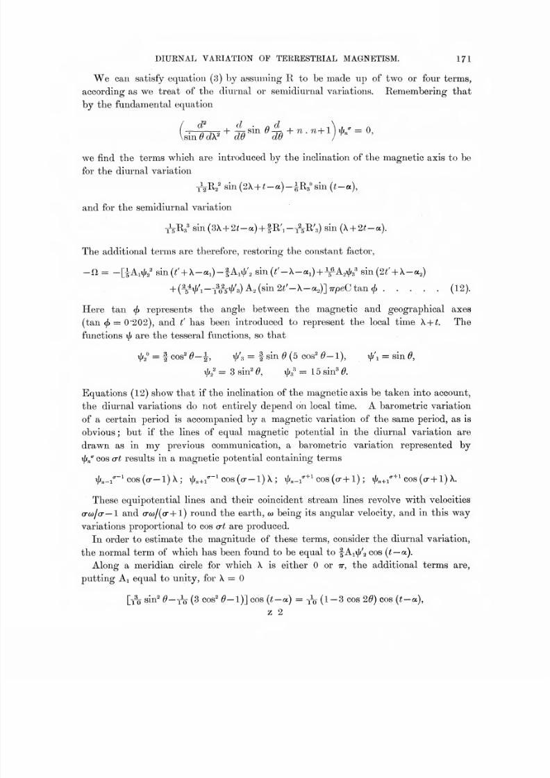
We can satisfy equation (3) by assuming li to be made up of two or four terms,
according as we treat of the diurnal or semidiurnal variations. Remembering that
by the fundamental equation
.sin 9 d\^ dd dO
we find the terms which are introduced by the inclination of the magnetic axis to be
for the diurnal variation
and for the semidiurnal variation
-i\Pv3' sin(3X+ 2^--a) +fR\—-f^-R',,) sin {\ + 2t-a).
The additional terms are therefore, restoring the constant factor,
-a = --[-i-Aii/// sin(«^' + X-ai)-fAii//'2 sin(^'-X-ai)+ -\^A2i//3'^ sin (2^' + X-a2)
+ p_^4^/^__M^y^) A, (sin 2t'-\-a.;)] npeC tan (/> . . . . . (12).
Here tan cj) represents the angle between the magnetic and geographical axes
(tan ^ = 0'202), and t' has been introduced to represent the local time X~\-t. The
functions i/> are the tesseral functions, so that
t/;/ = f cos' ^-> 1 , xfj',=: f sin ^ (5 cos' ^--1), fi
= sin 0,
t/,/= 3sin'^, xjji^ 15sin^6>.
Equations (12) show that if the inclination of the magnetic axis be taken into account,
the diurnal variations do not entirely depend on local time. A barometric variation
of a certain period is accompanied by a magnetic variation of the same period, as is
obvious ; but if the lines of equal magnetic potential in the diurnal variation are
drawn as in my previous communication, a barometric variation represented by
xfj/ cos crt results in a magnetic potential containing terms
r//^_i^""^ cos (or— 1)X; \jJn+/'~^ cos(a"— 1)X; xjjn-i''^^ cos(a-+l) ; i/z^+i'""^^ cos(or+l)X.
These equipotential lines and their coincident stream lines revolve with velocities
crco/cr-'l and oro)/(cr+l) round the earth, co being its angular velocity, and in this way
variations proportional to cos at are produced.
In order to estimate the magnitude of these terms, consider the diurnal variation,
the normal term of which has been found to be equal to fAii/z^g cos (^ — a).
Along a meridian circle for v/hich X is either or tt, the additional terms are,
putting Ai equal to unity, for X =
[i% sin' e—^ (3 cos' (9-1)] cos {t-a) =-f^ (1-3 cos 20) cos {t-a),
z 2

7/27/2019 Dinural Variation of Terrestrial Magnetism
http://slidepdf.com/reader/full/dinural-variation-of-terrestrial-magnetism 10/42
172 MR. ARTHUR SCHUSTER ON THE
and for \ = tt
[-1% sin^ (9+1 (3 cos^ ^-1)] cos {t-a) - } cos (t-a).
In these equations the numerical value 0*2 has been introduced for tan (/>.
At the equator the additional terms, therefore, have amplitudes f and ^ respectively,
as compared with the main diurnal term. The force to geographical west being
proportional to the potential, we may take these numbers to be the amplitude of the
westerly force variations. The main variation is proportional to sin cos 6, and has
zero value at the equator in the tropical region. The additional terms are therefore
the ruling terms at the equator. The horizontal force along the same circle has unit
amplitude, measured on the same scale, so that the new terms come well within the
range of our observational powers. It would be interesting to trace them, but it
should be remarked that only observations made near the equinox are suitable for
the purpose, as the seasonal terms, which yet remain to be discussed, would otherwise
interfere.
7. We may interrupt the progress of our investigation for a moment to inquire into
the magnitude of the electrostatic effect dependent on the potential S which was found
equal to —C-^^^.7^+l, leading to a vertical electric force Ga\jj/{n+l) a. In the
two cases which concern us, or = n, and i// has values at the equator which were found
to be S0a/7T and 15 a/rr respectively. It follows that the variation of vertical electric
force is of the order of 3 C.G.S. units, which is only 1 volt per 300 kilometres.
This may be disregarded.
8. The previous discussion has only taken the earth's vertical magnetic force
into consideration. The horizontal force causes, in combination with a horizontal
atmospheric oscillation, a vertical electromotive force, and so far as this produces
electric currents, their flow is in opposite directions in strata which are vertically
above each other. The magnetic effect is therefore of a smaller order of magnitude
than that due to vertical force.
9. In calculating the currents from the electric forces, I have applied Ohm's law,
and therefore neglected the effects of electric inertia ; but it is not difficult to
estimate the change of phase which results from self-induction. Using the equations
given by Maxwell'''' for spherical current sheets, we find that if R is the function
defined by equation (3), and <!> the current function,
where p is the conductivity, and L = (2n+ l)/47ra; provided that R is a surface
harmonic of degree n. If the latter function is proportional to cos Kt, we find in the
usual way/ , x ^ 47ra/cp
d) = p COS e cos (Kt— e), tan e = ~ f .
* See Clerk Maxwell, 'Electricity and Magnetism,' vol. II., § 672.
7/27/2019 Dinural Variation of Terrestrial Magnetism
http://slidepdf.com/reader/full/dinural-variation-of-terrestrial-magnetism 11/42
DIUENAL VAEIATION OF TEERESTEIAL MAGNETISM. I73
If we take the current sheets to be of finite thickness e, and p denotes conductivity
referred to unit volume, we must write
, AiraKoetan e = ^-~
.
2n+l
If pe has the value previously determined by the semidiurnal variation, I calculate
a retardation of 1 hour for the semidiurnal and about 1^ hours for the diurnal term.
The amplitude would be reduced by about 14 per cent. There are various causes,
notably the inequalities of conductivity, tending to diminish the retardation, so that
we may consider that self-induction would not cause a shift of phase amounting to
more than an hour, but it is in the ojoposite direction to that indicated by the
observations, if the barometric and magnetic oscillations are due to identical causes.
10. It is known that the air contains an excess of positive electricity, and the
question might be raised whether the oscillations of the atmosphere do notconvectively produce direct magnetic effects. If E be the total quantity of electricity
contained in a vertical column of unit cross section, and V, the velocity of air in that
column, supposed to be uniform, the total current in the atmosphere across a vertical
area of unit width is EV, and the magnetic force at the surface of the earth is of
the order of magnitude 27rEV. The quantity E must be equal and opposite to the
surface electrification of the earth, which itself is equal to Ff^Trv^, where v is the
velocity of light, and F the normal fall of potential, which we may put equal to
1 volt per centimetre, or to 10^. The magnetic force has therefore a magnitude
of order S'SYxlO^^^ If the velocity potential of the atmospheric oscillation is
A\///sin (T(X+t), the velocity in the two cases considered is greatest at the equator,
where its maximum rises to crAxfj/fa, which for the diurnal and semidiurnal change is
Ai/a and 6As/a respectively. It follows from the numerical values given in (8) that
the maximum equatorial velocities are 10 and 30 centims. per second respectively.
The magnetic forces due to such velocities are quite insignificant. In the literature
referring to the subject we frequently find it suggested that magnetic disturbances
are due to moving masses of electrified air, some writers even going so far as to say
that this has heen proved ; it may be demonstrated, on the contrary, that the assumed
cause is insufficient. For horizontal air currents this has just been demonstrated,
and the effects of ascending or descending currents are still less efficient. If a column
of air of cylindrical shape having as base a circle of radius r rises or falls with
velocity V, and it is imagined as an extreme case that the column extends indefinitely
in both directions, the magnetic force at the boundary is 27rrEV, where E is the
electric density. At the surface of the earth the ionisation is such that the free
electric charges of each kind amount to about 1 electrostatic unit per cubic metre.
Let us assume one kind to be suppressed altogether, so that this number represents
the electric volume density, or in electromagnetic measure 0'33xlO~^^ If r be
1 kilometre, and the velocity that of an express train, or 30 metres a second, the

7/27/2019 Dinural Variation of Terrestrial Magnetism
http://slidepdf.com/reader/full/dinural-variation-of-terrestrial-magnetism 12/42
174 MR. ARTHUE SCHUSTER ON THE
magnetic effect would be 6*3xl0~^ C.G.S. This is iiisigiiificant and leaves a good
margin for a greater sectional area of the ascending current, especially if it is
remembered that both our assumed velocity and the volume charges are many times
greater than is allowable. Magnetic effects due to the motion of electrified air musttherefore be ruled out as effective causes of either regular or irregular magnetic
changes.
11. The daily variation of the magnetic forces includes a strong seasonal term, the
amplitudes being greater in summer than in winter. In order to explain this term
according to the theory advocated, it is necessary to assume a greater electric
conductivity of the atmosphere in summer than in winter, or an oscillation of greater
amplitude, which is not, however, indicated by the barometric changes. That the
conductivity depends on the position of the sun, and may therefore vary with the
season, is suggested by the relation in phase between the diurnal and semidiurnal
terms, these terms combining together so as to leave the needle comparativelyquiescent during the night. Reserving the possible causes of the conductivity and
its dependence on solar position for further discussion, we may complete the theoretical
investigation by introducing a variable conductivity. The simplest supposition to
make will be that the conducting power in any small volume is proportional to the
cosine of the angle between the vertical and the line drawn to the sun, or, in other
words, proportional to the cosine of the angle, measured at the centre of the earth on
the celestial sphere, between the sun and the small volume considered. This angle
(oi) is expressed in spherical co-ordinates by
cos ft) = sin S cos ^ + sin # cos S COB X ...... (13),
where X is the longitude measured from the meridian passing through the sun, and 6
is measured from the pole, S representing the sim's declination. To put the assumed
law of conductivity into mathematical form, we write
p = po+ pi cos 0)>
If p^ = pq^ the conductivity would be zero at a point opposed to the sun, and this
is the highest admissible value of pi. In order to keep our investigation as general
as possible, I write
p = po (1+/ cos 6-\-y sin 6 cos X),
where y' and y may have any assigned values. The solution of our problem is
obtained if we can find values of S and R satisfying the equations
^ dk dd sin 6 dk|
^ (lA)
(id sin 6 dk dO
R will now give directly the current function which hitherto was denoted by poR.
7/27/2019 Dinural Variation of Terrestrial Magnetism
http://slidepdf.com/reader/full/dinural-variation-of-terrestrial-magnetism 13/42
DIURNAL VARIATION OF TERRESTRIAL MAGNETISM. 175
The general problem will be treated in the Appendix, where it is shown that for
practical purposes y and y^ may be treated as small quantities, the squares of which
may be neglected. The equations may then be written
' ok
d% 1.
., COS e/^
-
sin dX
—y cos 6—y sin cos X) -
.
dll•\
(1 —y cos 6—y sin 6 cos X)
sin 6 dX
dnV
dd
. (15).
J
Neglecting y and y\ our previous results give R in terms of i/i. Let Q,,^ be one
part of R thus obtained. The next approximation is found by substituting Q/ for R
in the terms of (15), which contain y and y'.
The complete value of R, as far as it depends on Q/, will then be Q/+K, where
R' is determined by
(/ cos 0+y sm cos X) -^-^ =/>o -^ +
^j^^
"N
V
(y^cos 6^+ y sm e^cos X) —y^ = Po-—n-JV TTT^ ^ ^ dd smtfak du
. . . (16).
J
In the two cases which specially interest us we must substitute for Q/ the values
respectively of Rg^ and pRi as determined by (5). The solution of (16) involves the
elimination of S^
Treating the terms containing y and y' separately, we find for R^ as far as it
depends on y\
i cot e "^'Sf + 4 sin d COS 0^) = --t7i . f^+ 1 . sin K,,dk' d0 d0
if R' is expressed as a series of harmonics, n being the degree of one of the terms of
the series.
The left-hand side may be transformed as shown in the Appendix, the result being
given by (25) ; we obtain in this way
^^ ^''"''''21
+
7""''^ ^^--+^""'^
^""+1^'''"- ^^'-0 = Sn(nf 1)K„.
R' is therefore expressible bj two terms,li'^„+i
and R'n-i,so that
{2n+1)(n+ 1) E\+i = y'n {n-cr+ 1) Q\+i,
{2n+ 1) w . RVi = r'{*^+ 1) («+o") QVi-
As regards the terms in y, the elimination of S' leads i;o
r[A cos Xi 4- COS X4 sin^ 4 ) Qn^ =:~tn{n+l) sin 0R\.\dX dX d0 d0,

7/27/2019 Dinural Variation of Terrestrial Magnetism
http://slidepdf.com/reader/full/dinural-variation-of-terrestrial-magnetism 14/42
176 ME. ARTHUR SCHUSTER ON THE
The left-hand side is transformed, as shown in the Appendix, the result being given
in (22). We thus find R^ expressible as a sum of four terms
2 (27^^h 1) n . R,„i--^^ = -y (n+l) Q.V'"',
2(27^+l)(n+l)Rn+l^~' = --7r^(n-cT-+l)(n--a-+ 2)Q^+i"-\
2(2n+l)n(7i-l)E^_i"-^ = y(9^-l)(?^+l)(^+c^)(n + o"-l)Q^„l"-\
For Q/ we must substitute ^GAi\jj2^ and -j^g-CAst/zs^ when treating of the diurnal
and semidiurnal variations respectively, where i//2^ and ii/3^ are the harmonics of type
and degree indicated which have the same factors as the current functions xjji^ and i//2^.
To get the magnetic potential, a further multiplication by — 47r(?i+l)/2n+ l is
required. We see that each barometric variation now leads to six terms in the
magnetic potential, the factors of —Trpo^ACO/ being collected in the following
table :
Diurnal Variation.
Velocity Potential : Aii///. Magnetic Potential : —Tipo^AiCSB/O/.
Values of B,,*^
:
71 = 1. n = 2. 71 = 3.
0- =
2
2
5'^
2
5
16
"105^
32 ,
315"^
8
315^
Semidiurnal Variation.
Velocity Potential : —7rpoeA2GtB/D./. Barometric Variation : A2»^2^.
Values of B^"" :-—
n =. 2. 71 = 3. n --= 4.
0- - 1
2
3
64
105^
32 ,
105^
32
105
2
"21^
Ay63^
1
63'^
C = Vertical force at geographical North Pole, measured upwards.
pQ— Electric conductivity of atmospheric shelL
e = Thickness of atmospheric shell.

7/27/2019 Dinural Variation of Terrestrial Magnetism
http://slidepdf.com/reader/full/dinural-variation-of-terrestrial-magnetism 15/42
DIURNAL VARIATION OF TERRESTRIAL MAGNETISM. 177
The main terms of the magnetic potentials Og^ and Og^ are now each affected by
both the diurnal and semidiurnal barometric variation, and their relative amplitudes
may differ considerably from those calculated on the assumption of a uniform con-
ductivity. If y has its maximum value, which is unity, we have for these two terms,
neglecting an unimportant difference of phase, and leaving out common factors,
The 24-hourly variation of terrestrial magnetism now takes the lead and as regards
westerly force is now 4*7 times as great as the semidiurnal variation, but the latter is
still too great for complete agreement with the facts, the observational ratio being 8*8.
This remaining discrepancy is not decisive against the accuracy of the assigned cause
in view of the uncertainty which attaches to the 24-hourly term in the barometric
variation as explained in § 4, and the considerations brought forward in the following
paragraph. There is the theoretical possibility of a further increase in the diurnal
term through a velocity proportional to Pg^ ; the motion specified by this potential
would give a barometric oscillation determined by the time of some definite meridian,
and though observations seem to indicate the existence of part of the oscillation being
of this nature, it is not likely that it is sufficiently great to produce a marked magnetic
effect.
12. A general review of the argument, even at the risk of repeating a portion of
what has already been said, may be appropriate, and is necessary to show how we are
naturally led to the theory here proposed. It will also serve to introduce the
consideration of the remaining difficulties and of the possibility of accounting for
the amount of ionisation necessary to explain the magnitude of the observed
effects.
Our object is to explain the cause of the periodic changes of the terrestrial magnetic
forces in so far as they depend on the position of the sun. The diurnal changes may
be represented as being governed by a magnetic potential O composed of terms of the
form fl/ cos a-(X+ ^), where 11/ is a surface harmonic; the observed vertical forces
show, as proved in my previous communication, that we must seek the cause of the
variation outside the earth's surface. Electric currents circulating in our atmosphere
and having a current function made up of terms which are respectively proportional
to O/ produce the required effect, and we are justified in assuming this—the simplest
explanation—to be also the correct one until it is shown to lead to contradictions.
The maintenance of the electric currents necessarily requires an electromotive force,
and their closed lines of flow dispose of any theory which would seek this force in a
static distribution of potential. Electric charges carried along by air currents have
VOL. CCVIIL—A, 2 A

7/27/2019 Dinural Variation of Terrestrial Magnetism
http://slidepdf.com/reader/full/dinural-variation-of-terrestrial-magnetism 16/42
178 ME. ARTHUR SCHUSTER ON THE
been shown to be insufficient to produce appreciable effects, and we are therefore
driven to look upon electromagnetic induction as being the only possible cause of the
observed effects, the earth's magnetism and atmospheric circulation being the active
agents. Assuming as most probable that atmospheric circulation is symmetrical northand south of the equator, the character of the magnetic variation shows that the
effective component of terrestrial magnetism has opposite signs in the two hemi-
spheres ; it must therefore be the vertical component which is active. We next put
the question : What must be the atmospheric circulation which under the action of
the vertical magnetic force produces periodical magnetic effects equal to those actually
observed ? Taking the average for the complete year, the leading terms of the
variable magnetic potential are Og^ cos (X+ ^) and Q^^ cos 2 {X4-^), the amplitude of the
diurnal term being equal to about eight times the amplitude of the semidiurnal one.
Calculation shows that ^2^ may be produced by a quasi-tidal atmospheric flow having
as velocity potential either xfji^ cos (X-i-t) or 1/%^ cos (X+ ^), while the semidiurnal termmay be produced by a flow having a velocity potential ^^^cos 2(X+^) or t|//cos 2(X+ ^).
But these velocity potentials are exactly what is required for the atmospheric waves
causing the daily changes of barometric pressure. The semidiurnal term of the
pressure change is the one least affected by local conditions, and its distribution over
the earth's surface is therefore accurately known. It is found that ilf/ is small
compared with t/i/. As regards the diurnal term having an amplitude at the equator
of only one-third of the semidiurnal one, it varies somewhat irregularly and the
relative importance of xpi^ and \p^^ is not well ascertained. Assuming the barometric
variation to be wholly due to i/zi^ cos(X+ ^) and t|// cos 2 (X-l-^), we may deduce the
magnetic variationand compare
it
withthe
observed changes. This has been thecourse of the investigation in the preceding paragraphs. It is found that the
calculated magnetic variations have a phase which lags behind the observed one by
about If hours, and this lag is slightly less for the diurnal term, but the difference is
insignificant in view of the uncertainties of the data. The amplitude of the calculated
diurnal term is about 2^ times as great as that of the semidiurnal one, while obser-
vation gives, as has already been stated, a ratio of 8 for the two terms. But if part
of the barometric variation is due to a term i/zy^—and there is some evidence that this
is the case-—agreement in the ratio of the two terms may be secured. There is,
however, a further cause tending to increase the semidiurnal magnetic variation. In
order to explain, on the basis of our theory, the difference in the magneticchanges
between summer and winter, we must assume that the conductivity of the atmosphere
is greater in that hemisphere which is more directly under the influence of the solar
rays. Assuming that the electric conductivity is proportional to 1 + cos oj, where a> is
the angle measured on the celestial sphere between the sun and the point considered,
the calculated semidiurnal term reaches a value which is 4*7 times as great as that of
the diurnal term, so that the term \po} is now called upon to a much smaller extent
for making up the deficiency in the diurnal term. The supposed inequalities of

7/27/2019 Dinural Variation of Terrestrial Magnetism
http://slidepdf.com/reader/full/dinural-variation-of-terrestrial-magnetism 17/42
DIURNAL VARIATION OF TERRESTRIAL MAONETlSxM. 179
conductivity, though helping towards a better agreement between the diurnal and
semidiurnal terms, are insufficient to account completely for the large excess of the
summer variation over that observed in winter. This inequality is expressed by D.^
for the semidiurnal variation and Og^ for the diurnal variation, and its relative
magnitude is indicated by the ratios OgYOg^ and Il//Hi^ respectively. The calculated
value of both ratios is shown by the tables in § 10 to be y = sin 8, where S is the
sun's declination. If we compare the variations during the six summer months with
those during the six winter montlis, we must substitute for sin S its average value,
which is about 0*26. On the other hand, the results of my previous communication
allow us to deduce the ratios ^.^lO^i and ^2!^! from the observations, and we find in
this 0*6 and 0*8 respectively, or values between two and three times as great as those
calculated from the assumed law of conductivity.
To explain the difference we might imagine some cumulative effect, so that in
midsummer the conduction would be greater than in winter even for the same elevation
of the sun, but our present knowledge does not justify us in assuming this to be the
case. I am inclined, therefore, to consider that the cause of the discrepancy lies
in the fact that, as already suggested in the introductory remarks, the oscillations
responsible for the barometric and magnetic phenomena are to some extent independent
of each other, affecting different layers of the atmosphere. There are theoretical
reasons why this should be so. It is now, I think, generally recognised that the
importance of the semidiurnal variation of the barometer is due to the fact that the
free period of the atmospheric oscillation, dependent on the velocity potential \\ii, is
very nearly equal to 12 hours. But it is to be remarked that if concentric layers of
the atmosphere be considered separately, there must be a considerable variation in
the free periods owing to differences of temperature, and in the highest regions, in
which alone electric currents of sufficient intensity can circulate, the temperature is
probably so low that the free periods would be more than doubled. If we take these
highest layers to oscillate to some extent independently, we should not therefore find
the semidiurnal variation stand out in the same way as it does for the lower layers.
Further, the inequalities of solar radiation in the two hemispheres near solstice ought
to cause an appreciable oscillation dependent on the velocity potentials i//^2 and \\fi.
The barometric variation due to i//3^ is unimportant compared with that due to i/zg^,
because although the forced period is 12 hours, the free period corresponding to the
motion involved in it has now a different value ; but in the upper layers the relative
importance of \\s^ would be increased, or, as it would be more correct to say, the
relative importance of \\ji disappears. This would account for the magnitude of the
seasonal term in the magnetic variation.
The suggested partial independence of the oscillations of the upper and lower
atmospheres may also explain the discrepancy of phase, which we found to be If hours,
but is in reality somewhat greater, owing to the fact that self-induction has been
neglected in calculating the phase. With the calculated conductivity, self-induction
2 A 2

7/27/2019 Dinural Variation of Terrestrial Magnetism
http://slidepdf.com/reader/full/dinural-variation-of-terrestrial-magnetism 18/42
180 ME. ARTHUR SCHUSTER ON THE
would cause a retardation of about one hour if the amplitude of oscillation is that
deduced from the barometric variation. If the amplitude in the conducting regions
is greater, the eflPect of self-induction is correspondingly less, because a smaller
conductivity would then be required to account for the magnetic change.
A few words should be said on the uncertainties of the data which serve as a test
of the proposed theory and which are derived from my previous calculation of the
variation potential. In deducing that potential I was practically obliged to confine
myself to the records of four observatories (Bombay, Lisbon, Greenwich, St. Petersburg),
all four being situated in the northern hemisphere ; and the year 1870 being the only
one for which records were available at all four stations, I had to base my calculations
on the figures for that year. Unfortunately, 1870 was a yea,r of unusual sunspot
activity and the magnetic records for that year cannot be taken as quite normal. It
is probable that if the average of a number of years were taken, the phases of the
components and their relative amplitudes might be somewhat altered;
but I do notthink that, as far as the averages for the whole year are concerned, the results of the
present investigation would be materially altered. A renewed discussion is, however,
very desirable, especially if observations in the southern hemisphere could be made
use of In my previous calculations I separated the summer from the winter months,
and assuming what is known to be approximately the case, each hemisphere to
behave alike when the sun occupies corresponding positions, I was enabled to form an
expression of the potential applicable for the whole world simultaneously. But this
is admittedly a defective process, and in drawing the equipotential curves I was
careful for this reason to use only the averages taken over the whole year and to
make no attempt to separate the two hemispheres.Voisr
Bezold, wholater,
basinghis calculations on my figures, effected this separation, is often quoted as having thus
completed my own investigation, but his extension of my work, for the reason given,
seems to me to be deceptive and to push too far the observed approximate symmetry
in the two hemispheres. What I now regret, however, is that I did not divide the
year into four parts instead of two, as Dr. Chrbe's results seem to show that the time
of equinoxes deserves special consideration.
If the views here brought forward are correct, all peculiarities of the barometric
variation should be reproduced in the magnetic effect, though we must remember
that the converse does not hold, and that peculiarities of the magnetic effect
depending partly on variations of electric conductivity need have no counterpart in
the barometric changes. Thus the greater amplitude of the magnetic variation
between summer and winter has already been ascribed to increased conductivity
of the atmosphere during the summer. The close relationship between the two
phenomena is confirmed by the increased amplitude observed in both near the time
of equinoxes. The diurnal period of barometric pressure is known to have maxima
at these epochs, and the valuable researches of Dr. Chree have shown that these
maxima are also found in the diurnal variation of the magnetic element. If we take
7/27/2019 Dinural Variation of Terrestrial Magnetism
http://slidepdf.com/reader/full/dinural-variation-of-terrestrial-magnetism 19/42
DIURNAL YAEIATION OF TEERESTRIAL MAGNETISM. 181
the variation of declination as characteristic, Dr. Chree's formula for the semidiurnal
term, leaving out the annual variation, is :
SD - 1-82 [1 + 0-137 sin (2^ + 271'')],
where t is measured from the beginning of January and each month counts as
30 degrees- The corresponding term in the barometric formula is, according
to Hann,^
hp = 0-988 [1 + 0-061 sin (2^+ 293-4)],
but if I understand the formula correctly, the time here is counted from the middle
of January. To make the equations correspond, we must therefore diminish the
angle in the last equation by 30 degrees, reducing it to 263 '4 degrees, in close agree-
ment with that given by Chree, the phase angle for the equinox being 265 degrees.
The maxima of horizontal force occur, however, a fortnight later, so that too muchvalue should not be given to this agreement ; the effect in amplitude is only about
half for the barometric variation ; but questions of conductivity may affect this ratio.
A remarkable feature distinguishing the barometric change is the maximum which
takes place simultaneously in both hemispheres early in January when the earth is in
perihelion. According to the theory here discussed, a corresponding annual inequality
should show itself in the magnetic variation, though the effect would be partially
masked in the northern hemisphere by the changes of conductivity, and could only
be ascertained by a comparison of the annual terms in the two hemispheres. We
should expect the difference between winter and summer to be more marked in the
southern hemisphere, because there the effects of conductivity would act in the samedirection as the effects of diminished distance from the sun. It is much to be desired
that some systematic attempt should be made to investigate the lunar influence on
the magnetic changes, for we possess at present only the vaguest information as to
how the different components of magnetic force are affected. It is quite possible
that the effects may depend on a tidal disturbance of the upper regions of the
atmosphere. If so, we may expect to get a valuable test of our theory by their
investigation.
13. We are now prepared to discuss the magnitude of the conductivity required
in order that the proposed theory should be tenable. If equations (9) and (10) are
compared with each other, and the correction discussed in § 5 be applied, we find
from the semi-diurnal term
p(3 = 3xl0"'.
The first question which arises is the value to be assigned to 6. Observations of
the aurora borealis conducted by the Danish expedition under the late Mr. Paulsen
have led to the conclusion that the arc of these luminosities is generally at a height
K- 'Met. Zeitsclirift,' 1898, vol. XV., p. 381.

7/27/2019 Dinural Variation of Terrestrial Magnetism
http://slidepdf.com/reader/full/dinural-variation-of-terrestrial-magnetism 20/42
182 MR. AETHtJR SCHtJSTER ON THE
of 400 kilometres.^ The height of meteors when they become luminous is as a
rule over 100 kilometres, but there is one case on record in which a height of
780 kilometres was found. We may therefore take 300 kilometres as an outside
limit for e, giving the value of 10"^^"^ as the lower limit for the conductivity. This
no doubt is a high value, and there may be some hesitation in accepting it as a
possible one. Mr. C T. R. Wilson has, however, already drawn attention to the
fact that at high altitudes we must, with the same ionising power, expect a much
increased conductivity, for the ionic velocity due to unit difference of potential varies
inversely with the pressure. If, further, as the experiments indicate, the ionising
power and rate of recombination of ions both diminish directly as the pressure, it
would follow that when the pressure is only the millionth part of an atmosphere the
conductivity should be for the same ionisation a million times as great as at the surface
of the earth.
Researches on the conductivity of gases generally give relative measures, so that it
is not always easy to infer its value in C.G.S. units, but I think the following
examples will give an idea of the order of magnitude involved.
The quantity of electricity in the form of ions of each kind under normal conditions
at the surface of the earth is 0*33 x 10"^^ in electromagnetic measure. To obtain the
conductivity the figures must be multiplied by the ionic velocity per unit fall ol
potential, the sum of the velocities of both kinds of ions being 3xl0"l The con-
ductivity of air at the surface of the earth is therefore under normal conditions 10~^^
Gerdien, in one of his balloon ascents, determined the conductivity at a height oi
6000 metres and found it to be 2x10"^*, which, as far as it goes, confirms the con-
clusion that the conductivity is inversely proportional to the density. At a height
such that the pressure is one dyne per square centimetre, and assuming that the
recombination of ions is not materially afiected by the low temperature, we should
thus get a conductivity of 10"^^, showing that, if the views discussed in this paper are
correct, the ionising power at great altitudes must be considerably greater than that
which acts on the air near the surface of the earth.
In speaking of the ionising efiects of Rontgen rays, Professor J. J. THOMSONf
states that even when the ionisation is exceptionally large the proportion of the
number of free ions to the number of molecules of the gas is less than 1 to 10^^.
From this I calculate the conductivity to be about 10"^*^ at atmospheric pressure.
Some experiments by Rutherford fix the conductivity of air, subject to the action of
radium having an activity 1000 times less than pure radium, to be 0*7 x 10"^^ under
normal conditions. These figures would give to the conductivity of air at a pressure
equal to that of a millionth atmosphere a magnitude comparable with that required.
We know of much more powerful ionisers than the Rontgen tube or even radium.
An electric discharge itself is sufficient to ionise a gas, as I proved as far back as
^ ^Rapports du Congres International de Physique/ vol. III., p. 438 (1900).
t ' Conductivity of Electricity through Gases,' p. 256.

7/27/2019 Dinural Variation of Terrestrial Magnetism
http://slidepdf.com/reader/full/dinural-variation-of-terrestrial-magnetism 21/42
DIURNAL VARIATION OF TERRESTRIAL MAGNETISM. 183
1887. Data supplied by H. A. Wilson^ show that in the positive column of a
vacuum tube the conductivity reaches the value 10"^^ and the kathode glow is even
more highly conducting. The same author has experimented with air ionised in
contact with hot platinum, and the data supplied by his diagramsf allow us to fix the
conductivity of such air as about 4x 10~^^ at a temperature of 1080°.' When the air
was charged with the spray from a 1 per cent, solution of a potassium salt, the
conductivity rose to 1*4 x 10~^^, the temperature being 1200°. The conductivity of a
Bunsen burner has been measured by Gold and found to be 8xlO~^l In view of
these figures, which all apply of course to atmospheric pressure, we ought not, I
think, to reject the value of 10"^^ as an impossible one for the conductivity of air at
high altitudes, but it is necessary to inquire into causes which produce so strong an
ionisation.
The increased intensity of the magnetic variation during the summer months
suggests directly that we are dealing Math a solar action. This action may be simply
an effect of radiation or it may be due to an injection of ions into the atmosphere.
The former hypothesis is the one which presents itself as the most natural one,
though the coronal streamers lend some countenance to the second view, which has
often been put forward and sometimes even pressed in support of wildly speculative
theories.
Ultra-violet radiation is known to ionise air in contact with metallic surfaces, but
the evidence is somewhat conflicting as to the effect of radiation on the air itself
Unless the air is absolutely free of dust, the observed action may be due to the
illumination of the dust and not of the air. Dust-free air is so transparent to
luminous radiation that it would not be surprising if the ionising effect would
disappear, as some experimenters believe it to do, when proper precautions are taken.
On the other hand. Dr. V. Schumann has shown that air has a very strong absorbing
power for wave-lengths which are sufficiently short. Such short wave-lengths are
supplied by several metallic sparks, and are freely transmitted through hydrogen.
Nevertheless it seems difficult to believe that, even if emitted by the hottest portion
of the sun s envelope, they are not absorbed again by the surrounding cooler layers.
We are not, therefore, at present in a position to assert that sufficiently short wave-
lengths can enter the atmosphere and be absorbed in the outer layer, thereby causing
ionisation, but we know so little about the conditions of the uppermost layers that
we may reasonably retain the view that the powerful ionisation of the air, which we
must consider to be an established fact, is a direct effect of solar radiation.
If we turn to the possibility of a direct injection of ions by the sun into our
atmosphere, we have to deal with the alternatives of supposing that ions of both kinds
are introduced or only those of one kind. The second alternative must be rejected at
once^ because a simple calculation shows that the outward force due to the volume
•^ 'Phil. Mag.,' 1900, p. 512.
t' Phil Trans.,' vol. 202, p. 243 (1904).

7/27/2019 Dinural Variation of Terrestrial Magnetism
http://slidepdf.com/reader/full/dinural-variation-of-terrestrial-magnetism 22/42
184 ME. AETHUR SOHUSTEE ON THE
electrification of air necessary to account for the required conductivity would be more
than sufficient to overcome gravitation and to drive out the conducting portions at an
enormous rate. The injection, on the other hand, of a sufficient number of ions of
both kinds also presents difficulties on account of the large quantity of new matter
which would have to accumulate in our air, especially if it is considered that
recombination at a rapid rate would take place both in the journey from the sun to
the earth and in the passage through the different layers of the atmosphere. The
only alternative to ultra-violet radiation seems, therefore, to lie in the injection of ions
travelling with sufficient rapidity to generate other ions by impact. The air itself,
according to this view, would supply the raw material for the ionisation, the injected
corpuscles only acting as fertilisers. There are, of course, other possibilities, such as
the introduction of radioactive matter, or a spontaneous ionisation which may, if the
rate of recombination is slow, be very effective at a great height ; but that the sun
undoubtedly plays an important part in the process is shown not onlyby
thesummer
effect, but also by the periodic changes of the magnetic variation, which corresponds
with the sunspot cycle. I have held for many years and frequently expressed the
opinion that the relationship can only be explained satisfactorily on the supposition
that the electric conductivity at times of many sunspots is increased. Whether this
is a direct influence of the sun, or only an indication that an ionising influence is
brought into the solar system from outside at times of many sunspots, is a question
which everyone is likely to answer according to his individual views of the cause of
sunspot variability.
That the increase in the number of sunspots coincides with an increased conductivity
of the upper layers of the atmosphere is also indicated by the eleven years' period of
the aurora borealis. The distinguishing feature of the relationship seems to be this,
that auroral displays extend further into moderate latitudes when the solar activity
is great. An increase of conductivity is the simplest and most natural way of
accounting for the effect. The primary cause of the electric discharges which manifest
themselves in the aurora is still unknown. We may look for it, perhaps, in electro-
static forces which are always present, but causing a visible discharge only when their
intensity rises abnormally, the course and intensity of discharge being much affected
by inequalities of conducting power. On the other hand, there are other electromotive
forces of induction not discussed in the paper, such as those accompanying a general
drift of the atmosphere from west to east, which may well have something to do with
the cause of auroral displays. Or again, if interplanetary space contains sufficient
matter to be conducting, as I believe it must, there will be strong electromotive forces
acting in the earth's magnetic field between the conducting powers rotating with the
earth and those of interplanetary space.
Outbreaks of magnetic disturbances, affecting sometimes the whole of the earth
simultaneously, may be explained by sudden local changes of conductivity which may
extend through restricted or extenpve portions of the atmosphere, I have shown in
7/27/2019 Dinural Variation of Terrestrial Magnetism
http://slidepdf.com/reader/full/dinural-variation-of-terrestrial-magnetism 23/42
DIURNAL VARIATION OF TERRESTRIAL MAGNETISM. 185
another place that the energy involved in a great magnetic storm is so considerable
that we can only think of the earth's rotational energy as the source from which it
ultimately is drawn. The earth can only act through its magnetisation in combination
with the circulation of the atmosphere, so that magnetic storms may be considered to
be only highly magnified and sudden changes in the intensity of electric currents
circulating under the action of electric forces w^hich are always present.
Those currents only are discussed in this communication which produce periodic
variations in the magnetic elements, but there are also electromotive forces giving rise
to current functions which are expressed by zonal harmonics and cannot under
ordinary circumstances be observed, though any variation of conductivity between
summer and winter would produce an annual period.
One further consequence of the theory deserves to be noticed. The electric currents
indicated by our theory are sufficiently large to produce a sensible heating effect in
the low-pressure regions through which they circulate. They will protect, therefore,
the outer sheets of the atmosphere from falling to the extremely low temperatures
which sometimes have been assumed to exist there, and they may help to form the
isothermal layer which balloon observations have proved to exist at a height of about
50,000 feet.
Enough has been said to show the importance of the questions on which further
investigation of the diurnal variation must give valuable information. If the
fundamental ideas underlying the present enquiry stand the test of further research,
we are in possession of a powerful method which will enable us to trace the cosmical
causes which affect the ionisation of the upper regions of the atmosphere and which
act apparently in sympathy with periodic effects showing themselves on and near the
surface of the sun. It should be our endeavour to put the theory itself to a more
accurate test than can at present be done. The most promising line of attack seems
to me to be the investigation of the diurnal variation near the equator, where, as
explained in § 6, it should not only vary with local time, but possess a term depending
on the time of the meridian which passes through the magnetic axis. An exact
determination of lunar effects would also, as has already been pointed out, serve as
a valuable test of the theory.
PART II,
The problem to be solved may be stated thus : a spherical shell of fluid is animated
by a quasi-tidal motion and is under the influence of magnetic forces of w^hich only
the vertical components are considered. It is required to find the magnetic effect of
the induced currents if the motion is subject to a velocity potential \jj/ cos cr (k+ t— a),
where \jj/ is a surface harmonic, X the longitude measured from some standard
meridian towards the east, and t is the local time of that meridian. The conductivity
p of the fluid is not necessarily uniform, but we take it to be expressible in the form
p = p^j+pj cos d-{-p2 sin 6 cos (K-ht),
VOL. ccviii.—A. 2 B
7/27/2019 Dinural Variation of Terrestrial Magnetism
http://slidepdf.com/reader/full/dinural-variation-of-terrestrial-magnetism 24/42
186 ME. AETHUR SCHUSTEE ON THE
where # is the eolatitude, and X+i^ measures the difference in longitude between the
sun and the place at which p is required. The question is solved if we can determine
the current function of the electric currents which are generated by the fluid moving
through the magnetic field. The problem for constant conductivity has been treated
in the first part of this communication and the interest of a non-uniform conducting
power is confined to the case that the variability depends on the angular distance
between the sun and the point considered. If oj be this angle, the effect of the suns
radiation will be proportional to cos o> in the hemisphere subject to the radiation,
ie. for values of o> smaller than ^tt. If the induction is due to the ionising power of
the sun's rays, the rate of recombination of ions has to be considered, but unless this
rate is of a different order of magnitude from that observed near the surface of the
earth, the conductivity may be considered to be proportional everywhere to the
illuminating power. For values of w intermediate between ^tt and tt we must, then,
give zero value to the conductivity. By means of Fourier series we may now ex23ress
the conductivity in a series
Po —hi- COS o)-\ COS 2aj+TT OTT
(17)>
which satisfies the condition
p = p^o COS 0) for 0<a)< --, and p = for --
Zi Zi
o><7r.
Confining ourselves to the first two terms and substituting the value ofcos a> from (13)
in terms of the hour-angla of the sun and its declination, we obtain
P^o2
TT
4- 1" sin S cos ^+|- cos 8 sin 6 cos {\~\-t)
The conductivity has therefore the assumed form if we put
2 ,
po = - pV; pi == Vo sin 8 ; p^ = ip'o cos 8.
TT
Were we to adopt the simpler form and put the conductivity proportional to 1 + cos co,
so that it reaches zero value only at midnight, we should have to put
Pi po sin 8; p2 = po cos 8.
and m every case p can be expressed in terms of a series such as (17), our investiga-
tion by proper adjustment of the constants taking account of the first two terms.
The term in cos 2(ja might be taken into consideration without much difficulty should
that become necessary. The value of po can provisionally be put equal to unity and
re-iiitroduced at a later stage. Writing y = pi/po and y = P2/P0 we may therefore put
p =i+y cos^+ysin $ gob (k+ t) . (18).
7/27/2019 Dinural Variation of Terrestrial Magnetism
http://slidepdf.com/reader/full/dinural-variation-of-terrestrial-magnetism 25/42
DIUENAL VARIATION OF TEERESTEIAL MAGNETISM. 187
In order to avoid frequent interruption, I prove in the first instance a few formulae
of transformation which I have found of great utiHty in these investigations. I start
from the following equations denoted in my previous communications by Roman
letters, which it is convenient to retain :
{2n+l) cos 0Q,r = (n-o-+l) Q\+i + {n + o-)Q\,-i
(2n+l)sin^Q„' = Q„+i-+i-Q„_i''+i
. . . . . . ... . (A),
(B),
??^=(ri+(T)(n+<r-l)Q„_i'^-' + Q„_r^ . (D),sin 6
dd
Q,+^"+ ^^-c^+ 2) (n-cr+l) Q^+r'
(n+ o-)(n-or+l)Q/-^-Q/+' . .
(E),
(Hi).
Q/ denotes the tesseral function derived from the zonal harmonic P^ by the relation
Q/ = sin"^ ~rT 'where \x ~ cos 9.
Multiplying (D) by {n—(T-\-\) and (E) by (r^+ cr), and adding, we find, with the
help of (A),
(2n-f 1) (r^+ 0-) (^— o- 4-1) cos /9Q,;
2or
sin d^?n
= ~(n+o-) Q„+,""''-(«'-cr+l) Q(T+l
n-\
If in the formula (A) we substitute cr+l for cr, it becomes
(27^+l)cos^Q/^^ = (^-a-)Q,-,l^^^-f(7^+ o-+l)Q,V''.
From the last two equations we obtain, by subtraction and substitution of (Hi),
(271+1) cos ^^^--;^Qdv sm u
nSJw+i^ ~(^'^+ 1/ Vw-i
Now multiplying (B) by n ., (n + 1), and subtracting, we finally obtain
sin 6 cos 6de
n.n+l
.
sin^ ^Q/— crQ„'
27i+l ^"m
If on the right-hand side of (Kj) we substitute the values of Q^+i""^^ and Q^-i""^^
from D and E, we obtain a corresponding equation
sin 6 cos 6^^'
dOn.n+l
.
sin^ 9
.
Q/+ o-Q
, . (Kg),
i^j IB Ji
7/27/2019 Dinural Variation of Terrestrial Magnetism
http://slidepdf.com/reader/full/dinural-variation-of-terrestrial-magnetism 26/42
188 MR. ARTHUR SCHUSTER ON THE
A further useful transformation is derived from the equations
(2n+l) cr cos ^Q/ = (T (ti— cr+ 1) Q^i+i+ o" (r^+ cr) Q%,-i,
do
^
(2r^+ 1) sin d "^'~ = n . (n-a-+ 1) Q''n+i-0^+ l) (r^+ cr) Q^,-i.
If we subtract and add these equations, they reduce to
and
cr cos (9Q/— sin ^"^ = sin ^Q/"^'^ ......... (Li),
cr cos ^Q/+ sin ^--jk- = {'/^ + <t) (r^— cr+ 1) sin ^Q/""^ .... (Lg).
We shall require to find the effect of the operation
-^ COS Xj^+ cos X ~y^ sin^ d ^ )
Q/ ^^^ (^^—a) , , . . (19).
We omit, for the sake of shortness, temporarily the constant a, and divide the
operation into two parts, the first being
/ d/^ • d » d\cos X -j~^ + sin 6
-fh^^^ ^
~Th ^^ cos o-X.
From the fundamental equation relating to tesseral harmonics this is equal to
-|-ti.(B+l) sin^^Q/[cos(cr+l)X+cos(cr-l)X] .... (20),
The remaining part of the operation is
7
cr sin X sin o-XQ/+sin 6 cos 6 cos X cos crX ,^ 0/clu
= icos(or+l)X(sin(9cos^c?Q/-(rQ/) + |cos(o'--l)X(sin^cos^^^^^^^. (21).
If (20) and (21) are now added, and Ki and Kg are applied, we find the result of
the operation to be, restoring a,
^1^^{(ti-~l) (ti+ l)Q,„/+i~-B. 1^+ 2. Q.+i^'^i} cos {((r+l)X~-a}
2.2n+l
cos {((F— 1) X— a} . . . (22).
We may note that each of the equations used, and therefore the final results^
remains true for a- = 0, if we define

7/27/2019 Dinural Variation of Terrestrial Magnetism
http://slidepdf.com/reader/full/dinural-variation-of-terrestrial-magnetism 27/42
DIURNAL VARIATION OF TERRESTRIAL MAGNETISM. 189
This is in agreement with Rodriguez's theorem, if the definition of Q/ depending
on the operation
(1 -i^^fd"''^ {iM'-lY/2''n I dfi'n+ cr
is extended to negative values of cr, for in that case
"^^ -2^n^^ ^^ di^^
- /_1V.^ {n-cr)ld'"-'{,ji^-lY
^ ' Tn ! (n + o-)
!
' c^/i»+-
^ ^ (n+ o-)!^" • (23).
It follows that the operation (17), in the case where Q,," cos a replaces
Q/cos (crX—
a),reduces to
2 . 271+1^^^"^-^^^'^"^-^^^'^^"^'^^^'^"^^)^'--'-^^ [cos(X^a)+ cos (X+ a)].
eThis result may also easily be obtained independently, but in view of the ultimat
application of (22) it is important to include the special case in the general one.
It will be appropriate here to obtain another formula which will be used sub-
sequently. Let it be required to find
<""''W-P^»^^% ....... (24).
From the fundamental equation we find this to be equal to
-rt.^^4 1
.sin /9 cos (9Q/~sin^ /9^^,
and as
-r...t+l.cos^Q/=-!^^{(n-tc.)Q-,,, + (n-cr+l)Q^„,,}
and
(24) becomes equal to
* /I
-2;^{(^^+ 2)«(n-a-+l)Q^,, + (n-l)(r. + l)(n+a-)QV,}. . (25).
are
We are now in a position to attack our main problem. The equations to be solved

7/27/2019 Dinural Variation of Terrestrial Magnetism
http://slidepdf.com/reader/full/dinural-variation-of-terrestrial-magnetism 28/42
190 MR. ARTHUE SCHUSTER ON THE
where X and Y have the values given in (1), and for p we must substitute the
expression (18), remembering, however, that we must ultimately restore the factor pQ.
We may also temporarily omit the factor C in the expression for the electric forces.
To find the current function
Rwe must eHminate S, but owing to the fact that
pcontains 6 and X, this does not seem to be possible directly. The difficulty must be
turned by eliminating in the first place R, and if S is then found, R may be
determined from the first of the above equations. It may occur to the reader that Rmight be more directly obtained if the resistivity were introduced instead of the
conductivity. This is true, but the results are less valuable, as may be seen from the
fact that, as suggested above, the Fourier expansion may have to be applied to the
conducting power in so far as it depends on the position of the sun. If the resistivity
were introduced as the variable, the high and possibly infinite values which the factor
would take when the conductivity sinks low or vanishes would present difficulties
much greater than those met with by keeping the conductivity as the variable
quantity.
The elimination of R requires in the first instance the reduction of
i.e. of
Yh pX sin O-^r --- pY,clu dX
pi4xsin^+4Y)+Xsin^^+Y^\dtl dk I du dk
Introducing the values of X and Y, the operation reduces to
{l +y COS 6-i-y sin 6 cos X) sin 6-~-—y^ sin d cos 6 -^dk dk
dxjj
y cos 9 ( cos 6 cos X -—- —sin ^ sin X
The part independent of y and y is
d\p— sin ^-™- = —cr sindib/ cos (crX— a).
dk
dxjj\
dd
The part depending on y^ is
2y sin 9 cos ^ "TY ~ —2yV sin 9 cos ^i/// cos (crX—a)c^X
= - 2vV sin e(^--^+l)^Vi+ 0?+cr)i|/V3
We are left with the part dependent on y, the factor of which is
cos X -~ (cos^ 9— sin^ 9) + sin 9 cos 9 sin X -^.dk d9
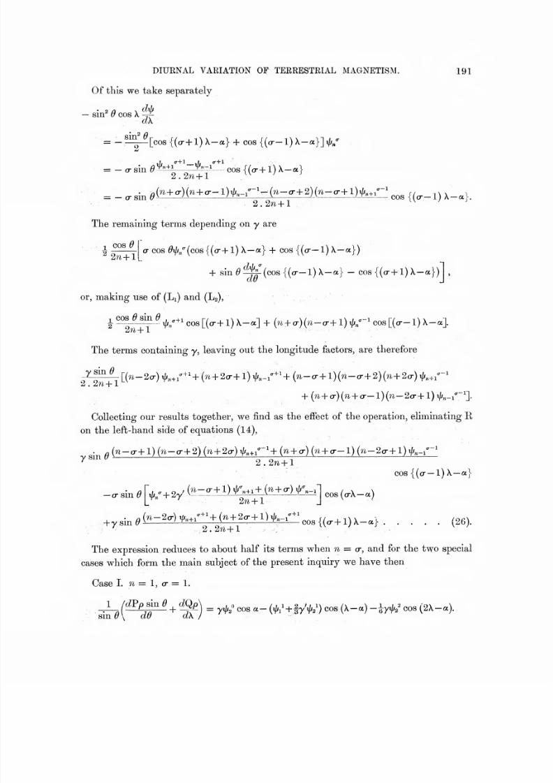
7/27/2019 Dinural Variation of Terrestrial Magnetism
http://slidepdf.com/reader/full/dinural-variation-of-terrestrial-magnetism 29/42
DIURNAL VARIATION OF TERRESTRIAL MAGNETISM.
Of this we take separately
sin^ 6 cos Xdk
sin^ 6—-[cos f(cr+l)X—a} + cos {(or— 1) X— a}]i|f„'
= — a- sin^
ar+l
n+1 Tm'-Icr+1
2.2^+1cos {(cr+1) X—a}
— cr smii%+ (r){n+ cr-l)t|f^--i^'"^r-(fi-cr+2) (n-0-4-l)i/y,,.t-/ ^
"'.
"^
2.. 2n+l ,v-^
cos {(o-— 1) X— a}
The remaining terms depending on y are
1 ^^^ ^
^271+1cr cos ^t///(cos{(cr+l)X— a} + cos {(cr— l)X— a})
+ sin ^-^(cos {{o— 1)X— «} — cos{(cr+l)X— a})de
or, making use of (Li) and (Lg),
i.?.oi^ii^i^,^-+icos[(o-+l)X-a] + (« + a-)(ft-o-+l)t/r/-^cos[(o— l)X-aiU'?l "T" X
The terms containing y, leaving out the longitude factors, are therefore
-y-^^[{7i-2a)ijj,^r'^''+{n+2a-+l)xlJr,-r''^'+{n~a-+l){n-a2 . 271+
+ (l^+o)(n+ o-l)(f^— 2cr+l)t|^,,_x''™^].
Collecting our results together, we find as the effect of the operation, eliminating R
on the left-hand side of equations (14),
r sm 2.271+1
cos {((J— 1)X— a}
— cr sin $2fh-h 1 '' ^"
^.y gin ^ L^^^^)^^-^^^"-^ (B+ 2cr+ 1) ^|..„r ^ ^^^ ^(^^ ^^
^^^~^ .... (26).
2.2n+ l . „: • ^^ / ^ • ^ ^
The expression reduces to about half its terms when n = cr, and for the two special
cases which form the main subject of the present incjuiry we have then
Case I. n = 1, cr = 1.
1 MPp sin e_^dQp\ ^ ^^^o^og^_(^^i+|y^^iycos(\-a)-iyi/./cos(2X-«).
sin 6 d\

7/27/2019 Dinural Variation of Terrestrial Magnetism
http://slidepdf.com/reader/full/dinural-variation-of-terrestrial-magnetism 30/42
192 MR ARTHUR SCHUSTER ON THE
Case II. n = 2, cr = 2.
si^ '^-''W~^+^ = fy (-V'^+ '^a^) COS (\-«) - {2^i+iy'^i) cos (2X-«)
— |^yt//3^ COS (3X— a).
Our next step must be to find the expression resulting from the terms containing S
in the elimination of R.
We shall begin by assuming S to be a spherical harmonic of the form Q/, and
shall again take the parts depending on y, y separately. Independently of both
these quantities, we have
4 sin e^ + J—^ "^-^f= ~n .n+1. sin OQ/ .... (27).
da du sm d dk^ ^ '
As factor of y' we have
4 sin Q cos e^ + cot e ^$4-dd dd d\^
The value of this has been obtained under (25).
Finally, as factor of y, we have
-TT, sin^ 6 cos X -~- + y- cos \ i~^ .
du du dX d\
This is identical with the expression (19), the result of the operation being given
by (22).
If we collect our results, by adding the right-hand side of (27) to (25) and (22)
after applying the appropriate factor, we shall have obtained an expression for
It will appear that S can be expressed in the form of a series
O" = 00
S =Kn
COS aQ/ -f
S{fc/ cos {ok—
a)+/x/ cos (o-X-f-a)}
Q/. . .
(29),cr^l
where a is determined by the phase of the velocity potential i/;/ sin (crX— o"), which
rules the flow of matter in which the electric currents are induced. We shall avoid
the labour involved in the consideration of special cases if we write (29) in the form
or = + 00
S= S k/Q/ COS (o-X-a) . . . . . . . . (30).cr = — 00

7/27/2019 Dinural Variation of Terrestrial Magnetism
http://slidepdf.com/reader/full/dinural-variation-of-terrestrial-magnetism 31/42
DIUENAL VARIATION OP TERRESTRIAL MAGNETISM. 193
Adopting the definition (23) for Q/, where cr is negative, we may return to the
original form by replacing the /x coefficients with the help of
K„-- = (-l)<^(^-'^|^/./ (31).
If each term of (30) be subjected separately to the operation (28) and the results
collected, so that all terms depending on any one value Q/ are brought together, we
may express the result of the operation by a series of the form
cr = + 00
% E/Q/sin ^cos (o-X—a) .....,, (32),or =— 00
which must be equal to (26),
If we put
E/ = A/+B/y+C/r • • • (33),
we find
xjL^ —— ' ^ \ '" IJ- / i^fi • • • • • • • • • • • • • • • • • • • • \*^/>
g,_ (ti-l)(n+l)(n^o-) n{n+2){n+<T+l)'
.g.x
P^- (^-1)(^+1),,
^-.1 n.n+ 2^^ ^-1 7i.{n + 2){7i+a+l){n+ a"{-2) ^+i
"" ^ 2.2^-1""-'
2.2n + 3^-^^ "^
'^^2T27Z+
3'
_ (^-1) (^+1) jn-a) (n-cr-l)^ ,+i /^gx
The values of k which determine S may now be found by equating the factors of
sin 6Q/ in (33) to the corresponding factor of sin $\1;/ in (26), remembering, however,
that in the latter equation cr and n have the definite value belonging to the assumed
velocity potential. If, for the sake of cleai'ness, the type and degree of this velocity
potential be now denoted by r and m, we find
E,/=T 2(2m+l)E«,-i"~^=-(m+T)(m+T-l)(m-2T+l)y]
(2m+l)EVi=2T(m+T)y 2(2m4-l)E^+/"^=-(m+2r)(m-r+l)(m-T+2)7'
(2m+ l)E",,,+i=2T(m-T+ 1)7 2(2m+ l)E«,-i^''^= -(m+ 2r+ 1)7
2(2m+l)E,,+i^+^=-~(m-2T)y
y{S7).
If in any of these values of E the index is less than the suffix, that value may be
put equal to zero, as the tessera! function to which that coefficient applies is zero.
All other values of E/ are zero. If we take the case r = 1, m = 1, as an example,
we obtain from (33), (34), (35), and (36) a number of equations in which all values
of E/ may be put equal to zero excepting Ei\ Eg^ E^^, E^^ ; the values of these are
VOL. ccviii.—A. 2 o

7/27/2019 Dinural Variation of Terrestrial Magnetism
http://slidepdf.com/reader/full/dinural-variation-of-terrestrial-magnetism 32/42
194 MR. ARTHUE SCHUSTER ON THE
obtained from (37) and we thus find equation (33) for these special vakies of n and
to become 9^i_i.9^.Vi ^./3^o i8^2\_ .
a. ,2 , 40_.' ,2 , ../1..1 4.-1 t 120.- 3\
cr
1 i\u«-2 -t-y \^^/Ci -t-"7"K3 ;-t-y y-f-K^ —Ki )
= —y
fi^ 2 , 40^,' 2 , ^ /l^ 1 4^1, 120^3\__ 1^,
These and all similar equations in which the right-hand side is equated to zero are
sufiicient to determine the k coefficients, each in terms of a series proceeding by
powers of 7 and 7 . I proceed to show how the successive approximations may be
obtained. If 7 and y are both zero, the first of the above equations leads to k^ = \,
and, as the equation must hold for all values of 7, this gives us that portion of k^
which is independent of 7 and y\ The remaining equations tell us that there can
be no other factor k which has a term not containing 7 and 7 . The last three
equations contain k/ and they are the only equations out of the complete series
which contain this particular factor. Substituting its vakie as far as it has been
found and neglecting in the brackets all factors except ki\ because they must all
depend on 7 or 7, and therefore introduce quantities of the second order, we obtain
a set of three equations which determines those coefficients which involve the first
powers of these quantities. We are thus led to
k/-1 27 Ki--- sVy ;
k/- 'hy
No other coefficients can contain terms depending on first powers. If we now write
down all equations in which k^, k^, Ki occur, we may determine the terms involving
7^, yy and y^. Thus if the above equation involving k^ is reconsidered, we find that
in view of our knowledge just acquired k^ must contain terms in 7^ and y"^ satisfying
the equation o 1 , 1 ^2 12 a
The equations for E'3, £3^, Es"^ give
i2k/+W^/+r {%^i-\^'^-%-^t) = 0,
i2K3-^+y(¥'^r^+5/cr^)+r (l'cr^-|-'^4-^+io/c/-^^/c/) = 0.
The factors such as k^, Kf^, Kf^, which can only contain powers of 7 and y higher
than the first may be left out of account in solving these equations, and we thus find
all terms which contain 7^, y^ or 77'. We may proceed in this manner, gradually
working by successive approximations from lower to higher powers. The following
two tables contain the results, including all powers as far as the third, for the two
typical atmospheric motions represented by the current functions i/// and i//2^. For
convenience of use the /^ coefficients now replace the k coefficients with negative
indices,

7/27/2019 Dinural Variation of Terrestrial Magnetism
http://slidepdf.com/reader/full/dinural-variation-of-terrestrial-magnetism 33/42
DIUENAL VAEIATION OF TEREESTRIAL MAGNETISM. 195
Values of k/. (Velocity Potential = iffi^.)
n — 1
(T =
1
140
11
11
2^80^ 40^
9. ^ ./2
2
12^^
89
302411
189
yt
_L89
36'^ 48x189 125
48x189
1 121yt
25
72' 189x192' 96x189
' 97 7^
77
1
_2
45
7
77
1
270 ' 1357
1
1080r
4
J- q J- ta
168^ 42^^
1
280^^'^420^
1 yB_J_
14x720' 14x180 77/o
1
14x7207 7^^
1
72 x 2807s
Values of /x/. (Velocity Potential = t/;/.)
71 = 1 2 3 4
(T = 1
(T = 2
y2
80
64x189"^
f180
1' 2
240'^'^
1 y3
14x240^
Values of /c/. (Velocity Potential = i/igl)
71
cr ==
1
1
105
105
9 '
7-^7
7'
2
637^
1+A3 189
7^
189;7
7207^7
1
7133
73
18 ' 36 X 360 ' 36 x 360
i 00 /o
77^
1 11
45'^ "^1620'\i
o _L1
48 X 270
1
J11
-yO _i_.
43
180' 36x180' 16x36x45 77
Jl_
28
yi
240
1
7
77
1
420 ' 2107
1
168077
1
3360kt
5
10577
2
1
7350 ' 175
'9
77 ^
1 9X / 9 .•J
• 7 7 H525^ ^ 1575
7
1 1
7^ + -^Tk 1112600' 315
1
45 X 16807'
2 g 2

7/27/2019 Dinural Variation of Terrestrial Magnetism
http://slidepdf.com/reader/full/dinural-variation-of-terrestrial-magnetism 34/42
196 ME. ARTHUR SCHUSTER ON THE
Values of ju./. (Velocity Potential = i/zg^.
n = 1 3 5
0- - 11 3
105'^
29^,3 1 3
630^2x360^
The determination of S is only of interest as a stepping stone to the evaluation
of R. We must therefore return to the first of equations (14), and hy its means
determine cIKjdk as a series of harmonics in the normal form.
If we write the velocity potential ^\fJ sin (rX— a), we find by means of the formulae
of transformation previously introduced
^ c/X 2m+l ^ ^
+ S ??!•^ (2m+l)(2m+ 3)
^ ^ (2m-l)(2m+l) ^^ ^ ^
r ^2(2m+l)(2??^+ 3)
+ (m+ r) ^-%'^'--^^^^^ A yr cos {(t+ l)X-a}^
^2.(2m-l)(2m4-l)J ^ ^^^
^^
T-l
+ -!(m-Tl i\(^^+ ^) 0^+ ^+1)^^/ ^-(m-T+ 2)(m-T+3)i/f,,.,,
^^ ^ 2(2m+l)(2m+ 3)
+ (m+ T )
0^^+ ^-"l)(^^+ ^-"2)i/;,,_/"^--(m>^T)(m-T+l)i|/,r^^ ^
2.(2m-l)(2m+l)>
yrcos {(r— l)X~-a} . . {^7 bis).
As, omitting constant factors, i/// is equal to Q/, the tesseral function of type a and
degree n, we may now write
pGOB0^ = 2//Q
and tabulate those values of // which are not equal to zero. The following table is
constructed in this way.
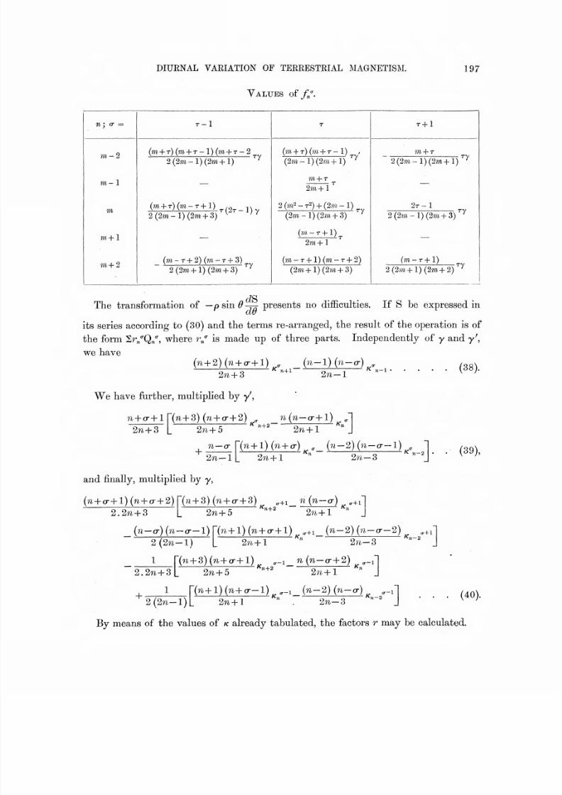
7/27/2019 Dinural Variation of Terrestrial Magnetism
http://slidepdf.com/reader/full/dinural-variation-of-terrestrial-magnetism 35/42
DIUENAL VARIATION OF TEERESTRIAL MAGNETISM. 197
Values of//.
n ; (T
m - 2
m-1
m
m + 1
w + 2
T~l
(m + t) (m+ T - 1) (??^ + T - 2
2(2w-l)(2m+l)~'^^
(m + T)(m-T+l) .^ -..
-^ ^ \^ ,
~- T (2t -1)72(2m-l)(2m + 3) ^
^^
__(m- T + 2) {m-T + 3)
2(2m+l)(2m+ 3)
'T"V
(w + r) (m + r- 1)
(2w-l)(2w+l)
2m +1
ry
2 (m^ - t2) -f- (2m - 1)
{2m - I) (2m -h 3)
'^^
(?/i -r + 1)
2m +1
(m--T + l)(m--T4-2)
(2m +1) (2m + 3)
T+1
W + T
2(2m-l)(2m+l) 7
2t~1
2 (2m -1) (2m +3)7
(m-T+1)
2 (2?7^+l)(2m.+ 2)
'^
y
The transformation of —psin^-y^ presents no difficulties. If S be expressed in
its series according to (30) and the terms re-arranged, the result of the operation is of
the form tr/Q/, where r/ is made up of three parts. Independently of y and y\
we have
(r6+ 2)(n + cr+l) (n-l) (fi-a) . .
"2;^T3''•''
2^r^l''^'^
.. . ^
{^^)^
We have further, multiplied by y\
2n+3
n (?^— cr+1)K,
'(^+ 3) (n+ cr+2) ^
2r^4-5''''''' "2^+1
^^— or r(n+l) (n+ cr) ^_ (n— 2) (^i— q-'
2n~-l 2^^n^''
'
2r?.-3+
1)../c «_?i~2 • • (39),
and finally, multiplied by y,
(n+ ar+l)(n + cr+ 2)
2.2^+ 3
"(ra + 3)(n+ (r+ 3) ^+i_ 11 (n-a) ,+1
2«+ 5"-^^
2n+l^n
{n—cr){n—cr—l)
2(2«,-l)
"
(ffl+ l)(w + cr+l) „+i _{n-2){n-(T
2n+l'*'"
2?^-3
-2)K
0-+ 1
71-2
2.2?i+3L
+
'(n+ 3)(n+ cr+l) ^_i_ ^(n-~or+ 2) ^^j"
2»+5 2?^ + l
2(2«,-l)
"
(w+1) (re+ o— 1) „ ^-1 (w-2) (w-o-),^ ,_i'
<:» . -t« o o '^ri-2
2n+l . 2n—3• • (40).
By means of the values of k already tabulated, the factors r may be calculated.

7/27/2019 Dinural Variation of Terrestrial Magnetism
http://slidepdf.com/reader/full/dinural-variation-of-terrestrial-magnetism 36/42
1 98 MR. ARTHUR SCHUSTER ON THE
R is expressible in the form
(r= Qo
R = S {p/ sin (crX— a) -hq/ sin {(tX+ a)] Q/,,.(r=i)
or, admitting negative values of cr, more conveniently by
(J-— +00
R = S p/Q/ sin (crX— a).(r= — 00
In the ultimate result we return to the q coefficients through the relation
^ -^ - (— iy+^ (^+ cr) ! ^
Equating the factors of Q/ cos cr (X— a) in (14), we now find
The calculation of r/ in its present form involves the summation of the expressions
(38), (39), and (40), the k factors being substituted out of the tables previously given.
The somewhat troublesome labour involved in this process may almost entirely be
avoided by a transformation of expression (38). Substituting A/ from (34) into (33),
we find
n . n + 1 . K/ =: E/-Bjy-C/y
,
and by means of this equation, when n+1 and n— ] are respectively substituted for
m, we obtain
where
P- ^ ^+^ + 1 V- _ {n-cr) ^,'' {n+l){2n+ 8)
''"' n{2n-l) ""-"
If the right-hand side of (41) replaces (38), and is added to (39) and (40), the whole
expression reduces to
"^"^ = ^»''+.7-;7TT&^>'
[x^r' + in-a) {n+ a+ 1) k„ "} -crVV].io , ft -T Ji
We have, therefore, the following very convenient expression which allows us to
calculate the p coefficients from the previously established values of k :
p/ = i(e/+/r) + ^^^^[iy{K/-^+(n-cr)(n+ cr+l)K/+^^-cryV] (42).
The first term on the right-hand side is zero, except for the cases where the type a

7/27/2019 Dinural Variation of Terrestrial Magnetism
http://slidepdf.com/reader/full/dinural-variation-of-terrestrial-magnetism 37/42
DIUENAL VAEIATION OF TEEEESTRIAL .MAGNETISM. 199
does not differ by more than 1 and the degree n by not more than 2 from the type
and degree of the original velocity potential.
For the calculation of these special cases the previous investigation furnishes the
necessary formulae. Confining ourselves tothe velocity potentials
xfj^^ and\jj2^,
we find
the requisite numbers collected in the following table :—
Values of e/+f/.
Velocity potential = if^]^.Velocity potential =
\Jy2^.
(T — 1 2 0" = 1'
2
10 ,
21^
4
15
2 .
35^
3
2
3
2 ,
5^
1
6
2 .
/ 45^
1
45 '^
n=2
. 3
4
1
3
70^
Equation (42) holds also for negative values of cr, but when a is smaller than —2,
it is more convenient to calculate the q coeflficients from the values of ju./ already
given. We find for this case
(±71
1
n , 71+Ylir {m/~'+ (^+ 0"+
1)(n-cr) /x/-^'} -(TyM
which, as may be expected, is identical with the equation connecting j9 and /c.
For o- = 1, (42) gives
and hence
jL nn . 71+Y
lir {(^-1) (^+2)/x/+/c,^}-//xV . . (43).
Our equations are not valid for the case cr = 0, because they depend on a division
by cr. The first of equations (14) from which we started containing R only in the
form dR/dk is obviously unsuitable to determine those parts of II which are
independent of X ; we must, therefore, have recourse to the second equation
dR ndxb ,dS
= p cos c^-^+p ~de dO ^ Bill 6 dX'
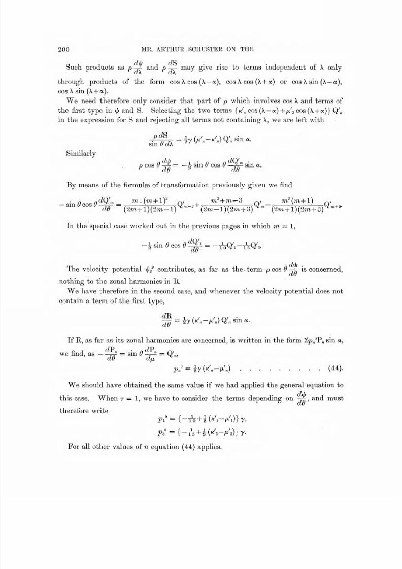
7/27/2019 Dinural Variation of Terrestrial Magnetism
http://slidepdf.com/reader/full/dinural-variation-of-terrestrial-magnetism 38/42
200 MR. AETHUR SCHUSTER ON THE
Such products as p -— and p -7— may give rise to terms independent of X only-
through products of the form cos X cos (X— a), cosXcos(X+a) or cos X sin (X— a),
cos X sin (X+ a).
We need therefore only consider that part of p which involves cos X and terms of
the first type in xfj and S. Selecting the two terms {/c^,, cos (X— a) +ju,'2 cos (X+a)} Q^^
in the expression for S and rejecting all terms not containing X, we are left with
= |y(/x^,,-~/<:',,)Q'^sina.
sin dk
Similarly
p cos -^ = — i- sin cos ---—?' sin a.^cl0
^d0
By means of the formulae of transformation previously given we find
-in CO- e^Q'--- - ^
»(^+ 1
)'
Q/I
^'+ ^^-3 q; m^(m+l) ^;smt/cost/^^^ -"(2m+l)(2m-l)^"^"'^(2m-l)(2m+ 3)^^'^ (2m+l)(2m + 3r"^''
In the special case worked out in the previous pages in which 7n = 1,
-1 sin e COS 6^ = -i-Q^-i-Q',.
The velocity potential \\fi contributes, as far as the ^ term p^osd-^ is concerned,
nothing to the zonal harmonics in R.
We have therefore in the second case, and whenever the velocity potential does not
contain a term of the first type,
^ = iy Wn-l^^n) Q^« sin a.
If R, as far as its zonal harmonics are concerned, is written in the form 2p«^P„ sin a,
we find, as ~ = sin -j-^ = Q^,
a0 dp.ny
We should have obtained the same value if we had applied the general equation to
this case. When r = 1, we have to consider the terms depending on -~^ and must
therefore write
K = {-ro+iK-/i)}7.
For all other values of n equation (44) applies.

7/27/2019 Dinural Variation of Terrestrial Magnetism
http://slidepdf.com/reader/full/dinural-variation-of-terrestrial-magnetism 39/42
DIURNAL VAEIATION OF TEEEESTEIAL MAGNETISM. 201
The tables which follow give the calculated values of p/ and g,,% and therefore
solve the problem as far as terms of the fourth order in y and y\ It will be noticed
that for unity, which is the highest admissible value of y and y\ all the factors
involviiiP' hi^rher powers than the first are so small that their effect falls much below
anything that observation is capable of showing. Hence the approximate calculation
given in Part I. is sufficient for all practical purposes.
Restoring constant factors, we may summarise the result of the previous investiga-
tion as follows :—
1. Notation.
Q,,*^ denotes the tesseral function sin^ 6 d^V.Jdix!'', where P„ is the zonal harmonic of
degree n, and 6 the colatitude.
C measured upwards denotes the vertical magnetic force of the earth's permanent
field at the geographical pole.
<3 is the thickness of the conducting atmospheric shell.
p is the conductivity, which is supposed to be variable and depending on 6 and the
local time \.-\-t, according to the relation /> = />o [1 +y^ cos /9+y sin 6 cos (X+OJ^ where
y and y^ are constant.
A/Q/ cos {or(X+f.)— a] is the velocity potential of the flow of air.
2. Oonchismi.
The current function II of electric flow induced under the action of the vertical
force C cos in the oscillating shell of air is then expressed as a sum
xvj = A.^ \j6p()
'o-= 30'
o-= oo
S _p/Q/ sin {or (X+ ;;)-«}+ S q/Q/ sin {a- {X+ 1) + a}
In order to obtain the magnetic potential of the variation caused by the flow of
air, a factor —4tw {n+l)/{2n+l) has to be applied.
The factors p/ and r// are given in the tables (including terms of the fourth order
of y and /) for the velocity potentials
A^iQ' = A^i sin cos {{X+t)-a}
rITlfl
A/Q/- = 3
A/sin^ ^ cos { 2 (X
+^- a
}
VOL. OCVIII.— 2 D
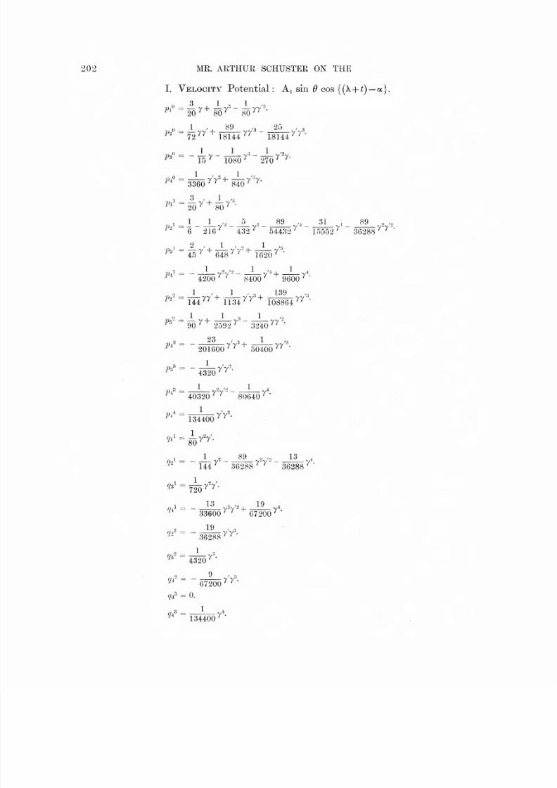
7/27/2019 Dinural Variation of Terrestrial Magnetism
http://slidepdf.com/reader/full/dinural-variation-of-terrestrial-magnetism 40/42
202 ME. ARTHUR SCHUSTER ON THE
I. Velocity Potential : Ai sin oos {{k+t)— a].
A 0,1 Q J. /9
^^^^20^+80^ 80>'^''"-
^"^ =72^^'' + 18144 ^''>'l8Hi^>-
fi = - jg7 -Jogo^'
"270^
^"
^'
, ^ 1 1 ,, 5 , 89 ,, 31 . 89 o .0
^"6 21G/ 432^ 54432^ 15.552'^ 36288 '^ ^
?'«^ =i5^+648^''>'"+T620^-
"^^
4200 ^ ^ 8400 ^ 9600 ^*
9 X I X t.')
p%- - ^ r + 2592^' " 3240^"^
'^'
-^^"^ "^ ~ 201600^^ 50400'^^''
i7,.'> r=: y y^,^ 4320 ^ ^
Po 1 9 ''•> xt
'
40320
'^ ^
80640
^
^ 134400^^
1 la/
I1 9 89 , ., 13 ,
144 ^ 36288 ^ ^ 36288"^
.1^1 o /
?B' = ^ry
33600' ^ 67200
^^36288 ^
"^
1
^^ 4320^
i) y /<>
^~^
67200 ^ ^
q^ = 0.
^^ 134400^

7/27/2019 Dinural Variation of Terrestrial Magnetism
http://slidepdf.com/reader/full/dinural-variation-of-terrestrial-magnetism 41/42
DIURNAL VAKIATION OF TERRESTRIAL MAGNETISM. 203
II. Velocity Potential: SAg^ sin^ ^ cos {2 (X + «)— a}.
v =105'^
i?2«= 0.
i'S»=
36'^
_?»/= 1 , o
oA ry--
12960"^
25920 '^ ^
I/O 157d
II210
'^^
^' 63^ 567 '^^ 567^'
X ^ 1 ,. 41 ^.^3 191 .
""^ 72'^''^ 51840'^''' 51840'^'^
^" 23625^' 31500^^'
09 ^
' " 63 '^ 567'''"'' 567'^'
i) ^ 1 /;> I o 1 /•> 9 OO A 11/J^
^^ 15 270 '^ 270^ 38880^ ^ 62208^ 9720^
«> 1 / , 1 f i),
1 /o
^*' = 35^ + 5600^^' -"-2100 ^-
^" 15750 '^ ^' 63000^ 23625^
'
g 1 / 4:1'3_i
i-OO /g^^' "
432'''''' "
311040'^''^
311040 ^'^
^^ " lio'^" 33600''''^ 8400^*
1 1q X / q X q ^
^94500
'^^
42000''^
^*'=-T3i40^'^'''-
1 1
^ 189000^'^ 283500^
'
^' "453600 ^
''''•
^/i^ "" ""
70'^^^'-
^^189
^
2 D 2
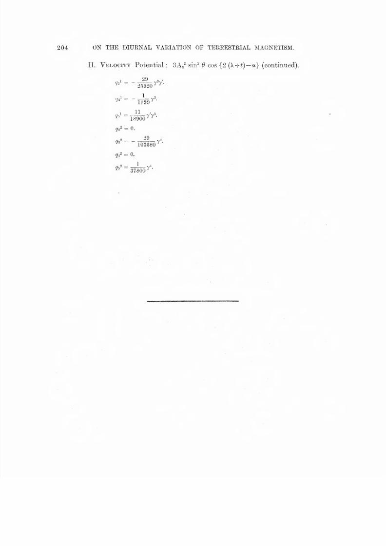
7/27/2019 Dinural Variation of Terrestrial Magnetism
http://slidepdf.com/reader/full/dinural-variation-of-terrestrial-magnetism 42/42
204 ON THE DIURNAL VARIATION OF TEREESTRIAL MAGNETISM.
II. Velocity Potential : ?>Ai sin^ 9 cos {2 (X + i)—a} (continued).
't>
-1 *J U ty f
o^ = 1t i^ Err: — —— '%/<-'
-] .1 X / QOr^' = - 7 7'\
^2'^ = 0.
?/ = 0.
•20
'' " "™
103680''"*
I
^' 37800 ^•
u tmittmmmaimmmmimi'mitntswMmmmmiesaiemBasai