Dijkstra’s AlgorithmSupervisor: Dr.Franek

Ritu Kamboj

0502560

Dijkstra’s Algorithm(Introduction)

It is named after a Dutch Computer Scientist Edsger Dijkstra.

This algorithm is used for solving the single- source shortest path problem.

The input of the algorithm consists of a weighted directed graph G and a source vertex s in G. G is a graph with nonnegative edge weights.

We will denote V the set of all vertices in the graph G. Each edge of the graph is an ordered pair of vertices (u,v) representing a connection from vertex u to vertex v. The set of all edges is denoted E. Weights of edges are given by a weight function w: E -> [0, ∞]; therefore w(u,v) is the non-negative cost of moving from vertex ‘u’ to vertex ‘v’.

The cost of an edge is the distance between those two vertices. For a given pair of vertices s and t in V, the algorithm finds the path from s to t with lowest cost (i.e. the shortest path).

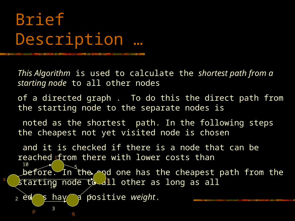
This Algorithm is used to calculate the shortest path from a starting node to all other nodes

of a directed graph . To do this the direct path from the starting node to the separate nodes is

noted as the shortest path. In the following steps the cheapest not yet visited node is chosen

and it is checked if there is a node that can be reached from there with lower costs than

before. In the end one has the cheapest path from the starting node to all other as long as all

edges have a positive weight.

Brief Description …

10 5

2

3

5

s t

r

p q

18

Application…

The algorithm works by keeping for each vertex ‘v’the cost ‘d[v]’ of the shortest path found so far

between s and v. Initially, this value is 0 for the source vertex s (d[s]=0) , and infinity for all other

vertices, representing the fact that we do not know any path leading to those vertices (d[v]=∞ for

every v in V, except s). When the algorithm finishes, d[v] will be the cost of the shortest path from s

to v or infinity, if no such path exists.

The basic operation of Dijkstra's algorithm is edge relaxation: if there is an edge from u to v, then

the shortest known path from s to u (d[u]) can be extended to a path from s to v by adding edge (u,v)

at the end. This path will have length d[u] + w(u,v). If this is less than the current d[v], we can

replace the current value of d[v] with the new value.

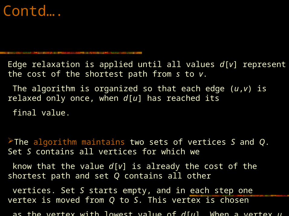
Edge relaxation is applied until all values d[v] represent the cost of the shortest path from s to v.

The algorithm is organized so that each edge (u,v) is relaxed only once, when d[u] has reached its

final value.

The algorithm maintains two sets of vertices S and Q. Set S contains all vertices for which we

know that the value d[v] is already the cost of the shortest path and set Q contains all other

vertices. Set S starts empty, and in each step one vertex is moved from Q to S. This vertex is chosen

as the vertex with lowest value of d[u]. When a vertex u is moved to S, the algorithm relaxes every

outgoing edge (u,v).

Contd….

Algorithm :

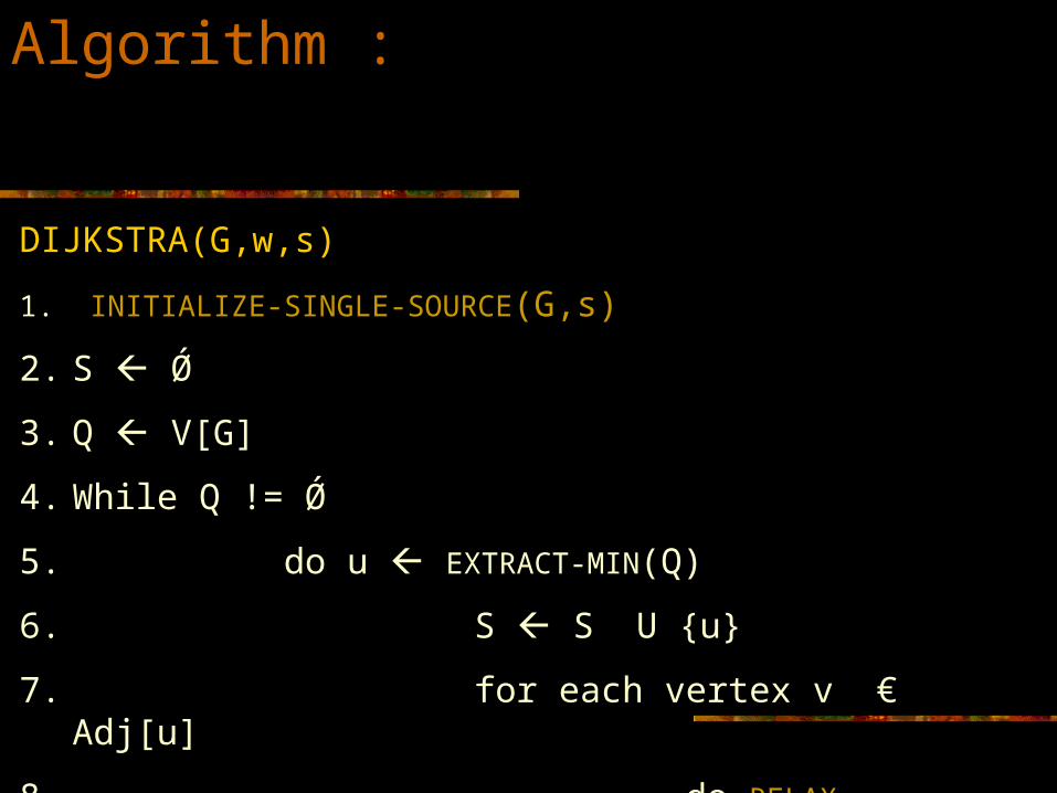
DIJKSTRA(G,w,s)

1. INITIALIZE-SINGLE-SOURCE(G,s)

2. S Ǿ

3. Q V[G]

4. While Q != Ǿ

5. do u EXTRACT-MIN(Q)

6. S S U {u}

7. for each vertex v € Adj[u]

8. do RELAX (u,v,w)

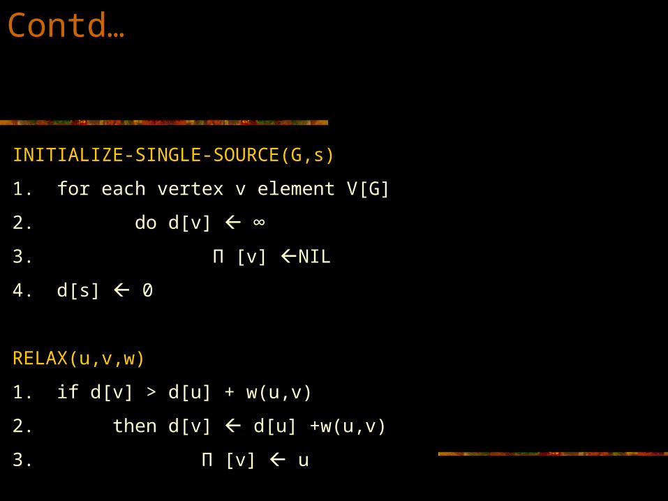
INITIALIZE-SINGLE-SOURCE(G,s)

1. for each vertex v element V[G]

2. do d[v] ∞

3. Π [v] NIL

4. d[s] 0

RELAX(u,v,w)

1. if d[v] > d[u] + w(u,v)

2. then d[v] d[u] +w(u,v)

3. Π [v] u

Contd…

Running time:

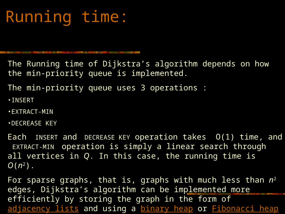
The Running time of Dijkstra’s algorithm depends on how the min-priority queue is implemented.

The min-priority queue uses 3 operations :•INSERT

•EXTRACT-MIN

•DECREASE KEY

Each INSERT and DECREASE KEY operation takes O(1) time, and EXTRACT-MIN operation is simply a linear search through all vertices in Q. In this case, the running time is O(n2).

For sparse graphs, that is, graphs with much less than n2 edges, Dijkstra’s algorithm can be implemented more efficiently by storing the graph in the form of adjacency lists and using a binary heap or Fibonacci heap as a priority queue to implement the Extract-Min function. With a binary heap, the algorithm requires O((m+n)log n) time, and the Fibonacci heap improves this to O(m + n log n).

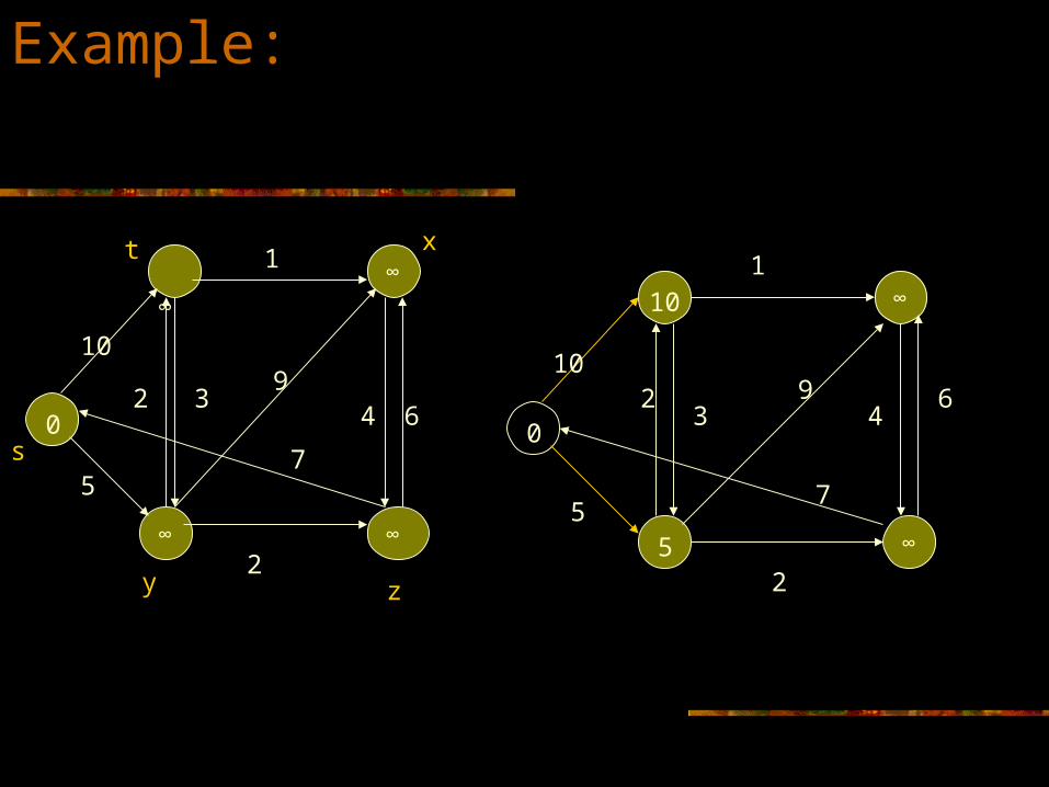
Example:

10

1

329

4 6

7

2

5

0

∞

∞

∞∞

s

y z

xt

0

10

1

64

7

2

55

10

392

∞

∞

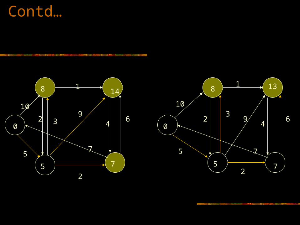
10

1

64

92 3

7

2

5

0

8

5

14

7

0

8

5 7

13

10

1

64

93

2

2

75

Contd…

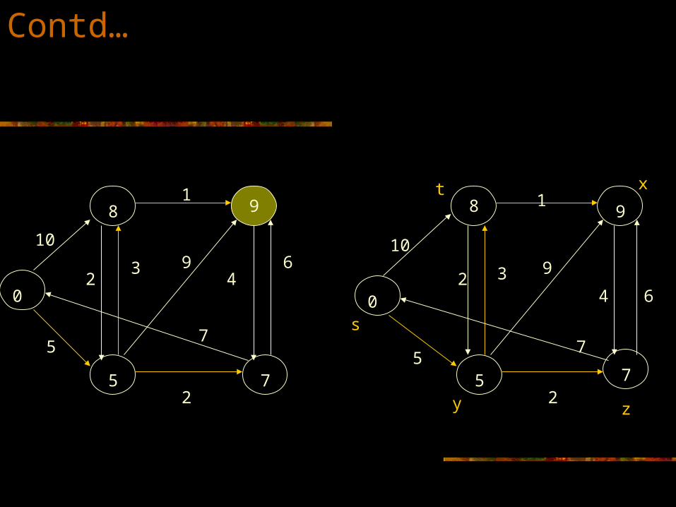
0

8

5 7

9

0

5 7

8 9

10

1

64

932

7

2

5

10

1

32

7

2

5

4 6

9

s

y z

xt

Contd…

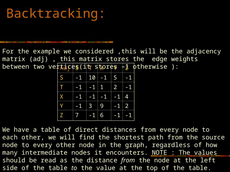
Adj S T X Y Z

S -1 10 -1 5 -1

T -1 -1 1 2 -1

X -1 -1 -1 -1 4

Y -1 3 9 -1 2

Z 7 -1 6 -1 -1

For the example we considered ,this will be the adjacency matrix (adj) , this matrix stores the edge weights between two vertices(it stores –1 otherwise ):

Backtracking:

We have a table of direct distances from every node to each other, we will find the shortest path from the source node to every other node in the graph, regardless of how many intermediate nodes it encounters. NOTE : The values should be read as the distance from the node at the left side of the table to the value at the top of the table.

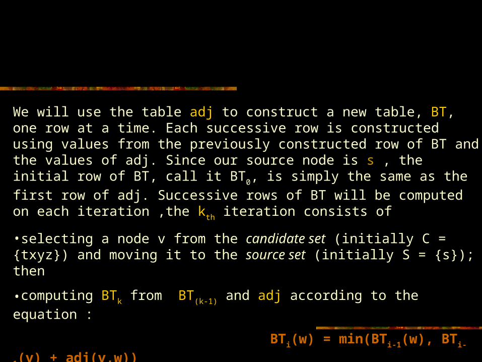
We will use the table adj to construct a new table, BT, one row at a time. Each successive row is constructed using values from the previously constructed row of BT and the values of adj. Since our source node is s , the initial row of BT, call it BT0, is simply the same as the first row of adj. Successive rows of BT will be computed on each iteration ,the kth iteration consists of

•selecting a node v from the candidate set (initially C = {txyz}) and moving it to the source set (initially S = {s}); then

•computing BTk from BT(k-1) and adj according to the equation :

BTi(w) = min(BTi-1(w), BTi-1(v) + adj(v,w))

The selection of w involves finding the node still in C that is closest to s according to the current row of BT.

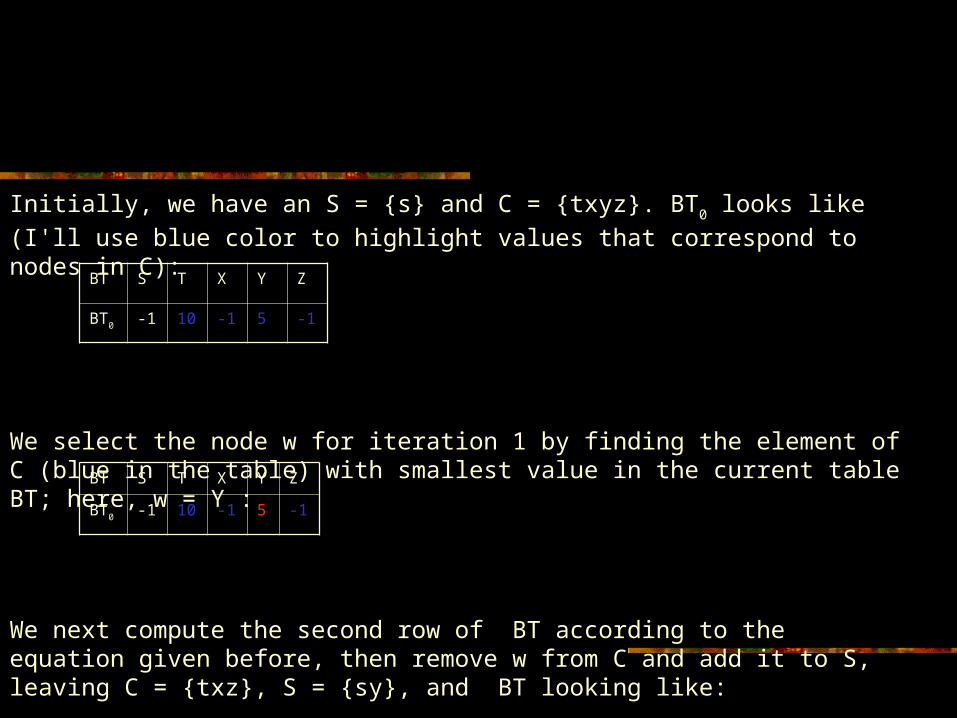
Initially, we have an S = {s} and C = {txyz}. BT0 looks like (I'll use blue color to highlight values that correspond to nodes in C):

We select the node w for iteration 1 by finding the element of C (blue in the table) with smallest value in the current table BT; here, w = Y :

We next compute the second row of BT according to the equation given before, then remove w from C and add it to S, leaving C = {txz}, S = {sy}, and BT looking like:

BT S T X Y Z

BT0 -1 10 -1 5 -1

BT S T X Y Z

BT0 -1 10 -1 5 -1

BT S T X Y Z

BT0 -1 10 -1 5 -1

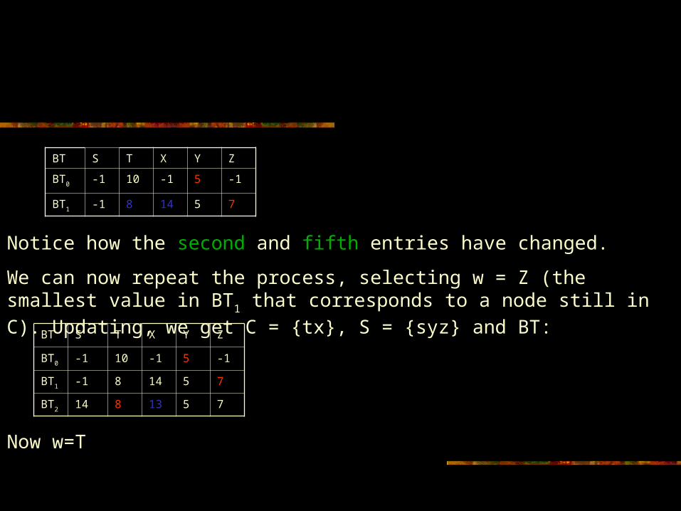
BT1 -1 8 14 5 7

Notice how the second and fifth entries have changed.

We can now repeat the process, selecting w = Z (the smallest value in BT1 that corresponds to a node still in C). Updating, we get C = {tx}, S = {syz} and BT:BT S T X Y Z

BT0 -1 10 -1 5 -1

BT1 -1 8 14 5 7

BT2 14 8 13 5 7

Now w=T

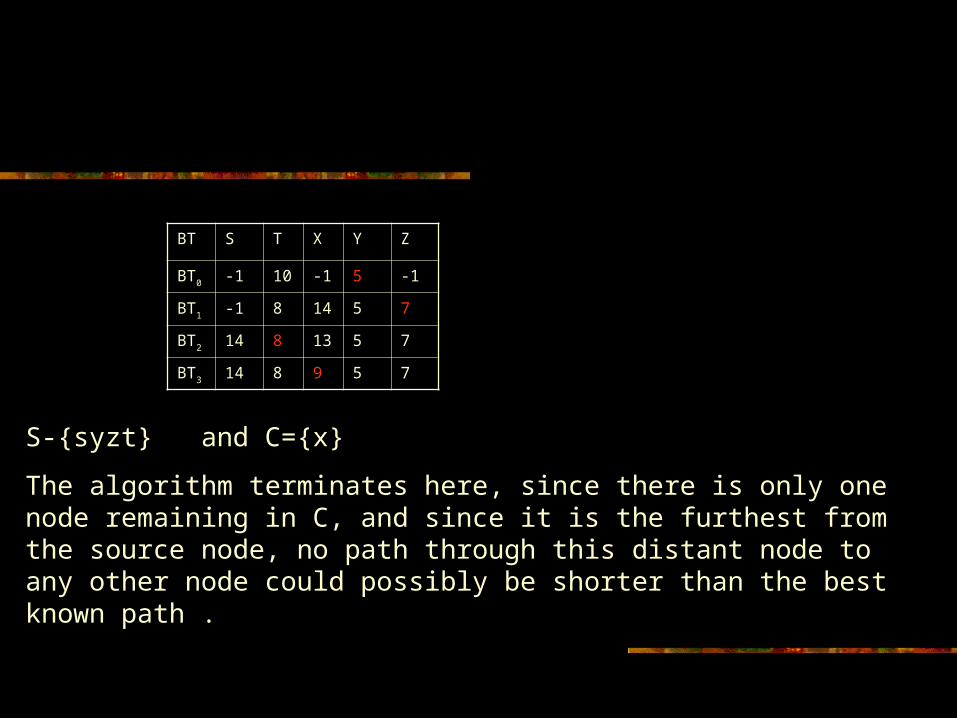
S-{syzt} and C={x}

The algorithm terminates here, since there is only one node remaining in C, and since it is the furthest from the source node, no path through this distant node to any other node could possibly be shorter than the best known path .

BT S T X Y Z

BT0 -1 10 -1 5 -1

BT1 -1 8 14 5 7

BT2 14 8 13 5 7

BT3 14 8 9 5 7

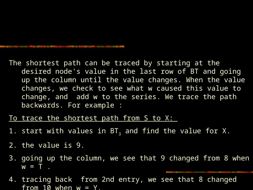
The shortest path can be traced by starting at the desired node's value in the last row of BT and going up the column until the value changes. When the value changes, we check to see what w caused this value to change, and add w to the series. We trace the path backwards. For example :

To trace the shortest path from S to X:

1. start with values in BT3 and find the value for X.

2. the value is 9.

3. going up the column, we see that 9 changed from 8 when w = T .

4. tracing back from 2nd entry, we see that 8 changed from 10 when w = Y.

5. tracing back from the 2nd entry, we see its value was fixed in BT0.

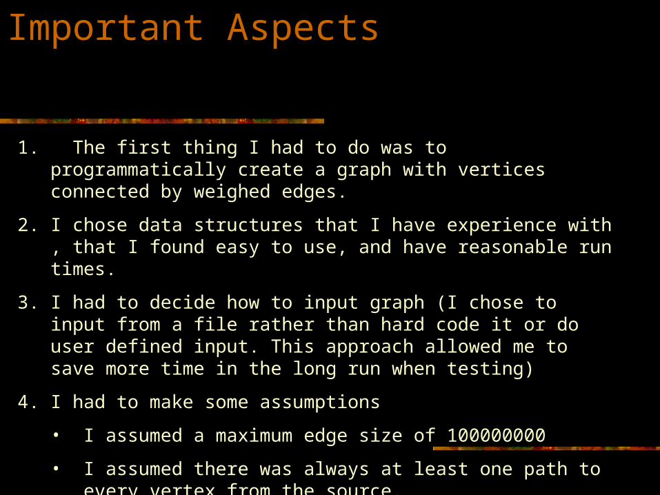
Important Aspects

1. The first thing I had to do was to programmatically create a graph with vertices connected by weighed edges.

2. I chose data structures that I have experience with , that I found easy to use, and have reasonable run times.

3. I had to decide how to input graph (I chose to input from a file rather than hard code it or do user defined input. This approach allowed me to save more time in the long run when testing)

4. I had to make some assumptions

• I assumed a maximum edge size of 100000000

• I assumed there was always at least one path to every vertex from the source.

• I assumed that edge lengths would not be zero

• I assumed there was no edge from a vertex to itself

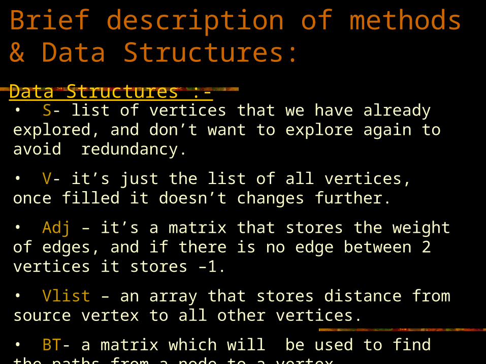
• S- list of vertices that we have already explored, and don’t want to explore again to avoid redundancy.

• V- it’s just the list of all vertices, once filled it doesn’t changes further.

• Adj – it’s a matrix that stores the weight of edges, and if there is no edge between 2 vertices it stores –1.

• Vlist – an array that stores distance from source vertex to all other vertices.

• BT- a matrix which will be used to find the paths from a node to a vertex.

Brief description of methods & Data Structures:Data Structures :-

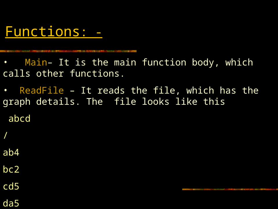
• Main– It is the main function body, which calls other functions.

• ReadFile – It reads the file, which has the graph details. The file looks like this

 abcd

/

ab4

bc2

cd5

da5

 

Functions: -

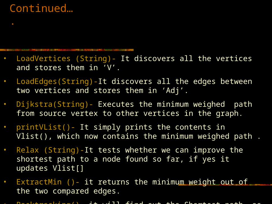
• LoadVertices (String)- It discovers all the vertices and stores them in ‘V’.

• LoadEdges(String)-It discovers all the edges between two vertices and stores them in ‘Adj’.

• Dijkstra(String)- Executes the minimum weighed path from source vertex to other vertices in the graph.

• printVList()- It simply prints the contents in Vlist(), which now contains the minimum weighed path .

• Relax (String)-It tests whether we can improve the shortest path to a node found so far, if yes it updates Vlist[]

• ExtractMin ()- it returns the minimum weight out of the two compared edges.

• Backtracking()- it will find out the Shortest path, as described just now.

Continued….

Weak Points :

• Using an adjacency matrix, the implementation uses more memory than if I were to use an adjacency list.

• If a graph exists with an edge weight greater than 100000000, then my implementation fails.

•If there is no existing path from the source vertex to one of the other vertices, then my implementation fails.

•If there are negative length edges in the graph , then my implementation fails.

Thank you!!!