dijkstra's algorithm on–line: an empirical case study from public

Dijkstra’s Algorithm On–Line:

An Empirical Case Study from

Public Railroad Transport

Frank Schulz, Dorothea Wagner, and Karsten Weihe

Universitat Konstanz, Fakultat fur Mathematik und InformatikFach D188, 78457 Konstanz, Germany

{schulz,wagner,weihe}@fmi.uni-konstanz.dehttp://www.fmi.uni-konstanz.de/~{schulz,wagner,weihe}

Abstract. Traffic information systems are among the most prominentreal–world applications of Dijkstra’s algorithm for shortest paths. Weconsider the scenario of a central information server in the realm of publicrailroad transport on wide–area networks. Such a system has to processa large number of on–line queries in real time. In practice, this problemis usually solved by heuristical variations of Dijkstra’s algorithm, whichdo not guarantee optimality. We report results from a pilot study, inwhich we focused on the travel time as the only optimization criterion. Inthis study, various optimality–preserving speed–up techniques for Dijk-stra’s algorithm were analyzed empirically. This analysis was based onthe timetable data of all German trains and on a “snapshot” of half amillion customer queries.1

1 Introduction

Problem. From a theoretical viewpoint, the problem of finding a shortest pathfrom one node to another one in a graph with edge lengths is satisfactorilysolved. In fact, the Fibonacci–heap implementation of Dijkstra’s algorithm re-quires O(m + n logn) time, where n is the number of nodes and m the numberof edges [8]. However, various practical application scenarios impose restrictionsthat make this algorithm impractical. For instance, many scenarios impose astrict limitation on space consumption.2

In this paper, we consider a different scenario: space consumption is not anissue, but the system has to answer a potentially infinite number of customerqueries on–line. The real–time restrictions are soft, which basically means thatthe average response time is more important than the maximum response time.The concrete scenario we have in mind is a central server for public railroad1 With special courtesy of the TLC Transport-, Informatik- und Logistik–Consulting

GmbH/EVA–Fahrplanzentrum, a subsidiary of the Deutsche Bahn AG.2 To give a concrete example: if a traffic information system is to be distributed on

CD–Rom or to be run on an embedded system, a naive implementation of Dijkstra’salgorithm would typically exceed the available space.

J.S. Vitter and C.D. Zaroliagis (Eds.): WAE’99, LNCS 1668, pp. 110–123, 1999.c© Springer-Verlag Berlin Heidelberg 1999

Dijkstra’s Algorithm On–Line 111

transport, which has to process a large number of queries (e.g. a server thatis directly accessible by customers through terminals in the train stations orthrough a WWW interface).

Algorithmic problems of this kind are usually approached heuristically inpractice, because the average response time of optimal algorithms seems to beinacceptable. In a new long–term project, we investigate the question to whatextent optimality–preserving variants of Dijkstra’s algorithm have become com-petitive on contemporary computer technology. Here we give an experience re-port from a pilot study, in which we focused on the most fundamental kindof queries: find the fastest connection from some station A to some station Bsubject to a given earliest departure time.

This scenario is an example of a general problem in the design of practicalalgorithms, which we discussed in [14]: computational studies based on artificial(e.g. random) data do not make much sense, because the characteristics of thereal–world data are crucial for the success or failure of an algorithmic approach ina concrete use scenario. Hence, experiments on real–world data are the methodof choice.

Related work. Various textbooks address speed–up techniques for Dijkstra’s al-gorithm but have no concrete applications in mind, notably [4] and [10]. In [13],Chapter 4, a brief, introductory survey of selected techniques is given (with astrong bias towards the use scenario discussed here). Most work from the scien-tific side addresses the single–source variant, where a spanning tree of shortestpaths from a designated root to all other nodes is to be found. Moreover, themain aspect addressed in work like [6] is the choice of the data structure for thepriority queue. In Section 2 below (paragraph on the “search horizon”), we willsee that the scenario considered in this paper requires algorithmic approachesthat are fundamentally different, and Section 3 will show that the choice of thepriority queue is a marginal aspect here.

On the other hand, most application–oriented work in this field is commercial,not scientific, and there is only a small number of publications. In fact, we arenot aware of any publication especially about algorithms for wide–area railroadtraffic information systems.

Some scientific work has been done on local public transport. For example,[12] gives some insights into the state of the art. However, local public transportis quite different from wide–area public transport, because the timetables arevery regular, and the most powerful speed–up techniques are based on the strictperiodicity of the trains, busses, ferries, etc. In contrast, our experience is thatthe timetables of the national European train companies are not regular enoughto gain a significant profit from these techniques.3

On the other hand, private transport has been extensively investigated inview of wide–area networks. Roughly speaking, this means “routing planners”for cars on city and country maps [2,3,5,7,9,11]. This problem is different to3 This experience is supported by personal communications with people from the

industry.

112 F. Schulz, D. Wagner, K. Weihe

ours in that it is two–dimensional, whereas train timetables induce the time asa third dimension: due to the lack of periodicity, the earliest departure time issignificant in our scenario. In contrast, temporal aspects do not play any role inthe work quoted above.4 So it is not surprising that the research has focused onpurely geometric techniques.

For completeness, we mention the work on variants of Dijkstra’s algorithmthat are intended to efficiently cope with large data in secondary memory. Chap-ter 9 of [1] gives an introduction to theoretical and practical aspects. As men-tioned above, the problems caused by the slow access to secondary memory arebeyond the scope of our paper.

Contribution of the paper. We implemented and tested various optimality–pre-serving speed–up techniques for Dijkstra’s algorithm. The study is based onall train data (winter period 1996/97) of the Deutsche Bahn AG, the nationalrailroad and train company of Germany. The processed queries are a “snapshot”of the central Hafas5 server of the Deutsche Bahn AG, in which all queries ofcustomers were recorded over several hours. The result of this snapshot comprisesmore than half a million queries, which might suffice for a representative analysis(assuming that the typical query profile of customers does not vary dramaticallyfrom day to day).

Due to the above–mentioned insight that the periodicity of the timetablesis not a promising base for algorithmic approaches, the question is particularlyinteresting whether geometric techniques like those in routing planners are suc-cessful, although the scenario has geometric and temporal characteristics. Wewill see that this question can indeed be answered in the affirmative.

2 Algorithms

Train graph. The arrival or departure of a train at a station will be called anevent. The train graph contains one node for every event. Two events v andw are connected by a directed edge v → w if v represents the departure ofa train at some station and w represents the very next arrival of this train atsome other station. On the other hand, two successive events at the same stationare connected by an edge (in positive time direction), which means that everystation is represented in the graph by a cycle through all of its events (the cycleis closed by a turn–around edge at midnight).

In each case, the length of an edge is the time difference of the events repre-sented by its endnodes. Obviously, a query then amounts to finding a shortestpath from the earliest event at the start station not before the earliest departuretime to an arbitrary arrival event at the destination.

The data contains 933, 066 events on 6, 961 stations. Consequently, there are933, 066 · 3/2 = 1, 399, 599 edges in the graph.4 In principle, temporal aspects would also be relevant for the private transport, for

example, the distinction between “rush hours” and other times of the day.5 Hafas is a trademark of the Hacon Ingenieurgesellschaft mbH, Hannover, Germany.


0

5000

10000

15000

20000

25000

30000

35000

0 100 200 300 400 500 600 700 800

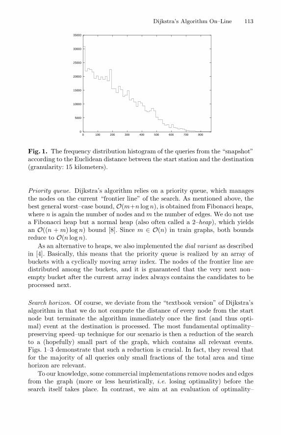
Fig. 1. The frequency distribution histogram of the queries from the “snapshot”according to the Euclidean distance between the start station and the destination(granularity: 15 kilometers).

Priority queue. Dijkstra’s algorithm relies on a priority queue, which managesthe nodes on the current “frontier line” of the search. As mentioned above, thebest general worst–case bound, O(m+n log n), is obtained from Fibonacci heaps,where n is again the number of nodes and m the number of edges. We do not usea Fibonacci heap but a normal heap (also often called a 2–heap), which yieldsan O((n + m) log n) bound [8]. Since m ∈ O(n) in train graphs, both boundsreduce to O(n log n).

As an alternative to heaps, we also implemented the dial variant as describedin [4]. Basically, this means that the priority queue is realized by an array ofbuckets with a cyclically moving array index. The nodes of the frontier line aredistributed among the buckets, and it is guaranteed that the very next non–empty bucket after the current array index always contains the candidates to beprocessed next.

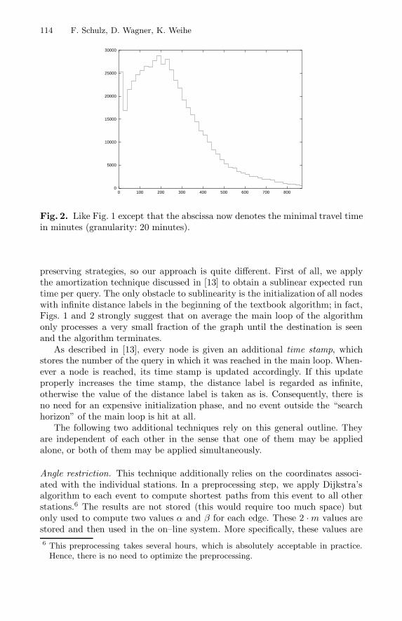
Search horizon. Of course, we deviate from the “textbook version” of Dijkstra’salgorithm in that we do not compute the distance of every node from the startnode but terminate the algorithm immediately once the first (and thus opti-mal) event at the destination is processed. The most fundamental optimality–preserving speed–up technique for our scenario is then a reduction of the searchto a (hopefully) small part of the graph, which contains all relevant events.Figs. 1–3 demonstrate that such a reduction is crucial. In fact, they reveal thatfor the majority of all queries only small fractions of the total area and timehorizon are relevant.

To our knowledge, some commercial implementations remove nodes and edgesfrom the graph (more or less heuristically, i.e. losing optimality) before thesearch itself takes place. In contrast, we aim at an evaluation of optimality–


0

5000

10000

15000

20000

25000

30000

0 100 200 300 400 500 600 700 800

Fig. 2. Like Fig. 1 except that the abscissa now denotes the minimal travel timein minutes (granularity: 20 minutes).

preserving strategies, so our approach is quite different. First of all, we applythe amortization technique discussed in [13] to obtain a sublinear expected runtime per query. The only obstacle to sublinearity is the initialization of all nodeswith infinite distance labels in the beginning of the textbook algorithm; in fact,Figs. 1 and 2 strongly suggest that on average the main loop of the algorithmonly processes a very small fraction of the graph until the destination is seenand the algorithm terminates.

As described in [13], every node is given an additional time stamp, whichstores the number of the query in which it was reached in the main loop. When-ever a node is reached, its time stamp is updated accordingly. If this updateproperly increases the time stamp, the distance label is regarded as infinite,otherwise the value of the distance label is taken as is. Consequently, there isno need for an expensive initialization phase, and no event outside the “searchhorizon” of the main loop is hit at all.

The following two additional techniques rely on this general outline. Theyare independent of each other in the sense that one of them may be appliedalone, or both of them may be applied simultaneously.

Angle restriction. This technique additionally relies on the coordinates associ-ated with the individual stations. In a preprocessing step, we apply Dijkstra’salgorithm to each event to compute shortest paths from this event to all otherstations.6 The results are not stored (this would require too much space) butonly used to compute two values α and β for each edge. These 2 · m values arestored and then used in the on–line system. More specifically, these values are6 This preprocessing takes several hours, which is absolutely acceptable in practice.

Hence, there is no need to optimize the preprocessing.


0

50

100

150

200

250

300

350

400

450

500

0 200 400 600 800 1000 1200

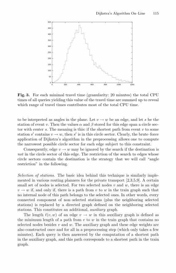
Fig. 3. For each minimal travel time (granularity: 20 minutes) the total CPUtimes of all queries yielding this value of the travel time are summed up to revealwhich range of travel times contributes most of the total CPU time.

to be interpreted as angles in the plane. Let v → w be an edge, and let s be thestation of event v. Then the values α and β stored for this edge span a circle sec-tor with center s. The meaning is this: if the shortest path from event v to somestation s′ contains v → w, then s′ is in this circle sector. Clearly, the brute–forceapplication of Dijkstra’s algorithm in the preprocessing allows one to computethe narrowest possible circle sector for each edge subject to this constraint.

Consequently, edge v → w may be ignored by the search if the destination isnot in the circle sector of this edge. The restriction of the search to edges whosecircle sectors contain the destination is the strategy that we will call “anglerestriction” in the following.

Selection of stations. The basic idea behind this technique is similarly imple-mented in various routing planners for the private transport [2,3,5,9]. A certainsmall set of nodes is selected. For two selected nodes v and w, there is an edgev → w if, and only if, there is a path from v to w in the train graph such thatno internal node of this path belongs to the selected ones. In other words, everyconnected component of non–selected stations (plus the neighboring selectedstations) is replaced by a directed graph defined on the neighboring selectedstations. This constitutes an additional, auxiliary graph.

The length `(v, w) of an edge v → w in this auxiliary graph is defined asthe minimum length of a path from v to w in the train graph that contains noselected nodes besides v and w. The auxiliary graph and these edge weights arealso constructed once and for all in a preprocessing step (which only takes a fewminutes). Each query is then answered by the computation of a shortest pathin the auxiliary graph, and this path corresponds to a shortest path in the traingraph.


0

20000

40000

60000

80000

100000

120000

140000

160000

0 5000 10000 15000 20000 25000 30000 35000 40000 45000 50000

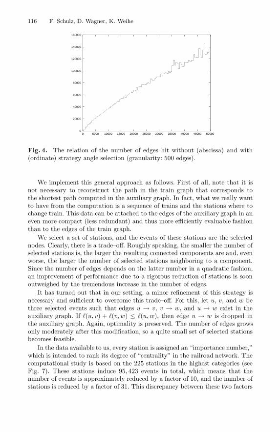
Fig. 4. The relation of the number of edges hit without (abscissa) and with(ordinate) strategy angle selection (granularity: 500 edges).

We implement this general approach as follows. First of all, note that it isnot necessary to reconstruct the path in the train graph that corresponds tothe shortest path computed in the auxiliary graph. In fact, what we really wantto have from the computation is a sequence of trains and the stations where tochange train. This data can be attached to the edges of the auxiliary graph in aneven more compact (less redundant) and thus more efficiently evaluable fashionthan to the edges of the train graph.

We select a set of stations, and the events of these stations are the selectednodes. Clearly, there is a trade–off. Roughly speaking, the smaller the number ofselected stations is, the larger the resulting connected components are and, evenworse, the larger the number of selected stations neighboring to a component.Since the number of edges depends on the latter number in a quadratic fashion,an improvement of performance due to a rigorous reduction of stations is soonoutweighed by the tremendous increase in the number of edges.

It has turned out that in our setting, a minor refinement of this strategy isnecessary and sufficient to overcome this trade–off. For this, let u, v, and w bethree selected events such that edges u → v, v → w, and u → w exist in theauxiliary graph. If `(u, v) + `(v, w) ≤ `(u, w), then edge u → w is dropped inthe auxiliary graph. Again, optimality is preserved. The number of edges growsonly moderately after this modification, so a quite small set of selected stationsbecomes feasible.

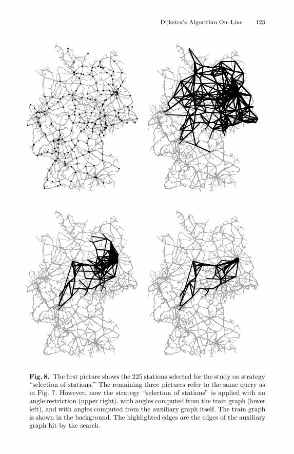
In the data available to us, every station is assigned an “importance number,”which is intended to rank its degree of “centrality” in the railroad network. Thecomputational study is based on the 225 stations in the highest categories (seeFig. 7). These stations induce 95, 423 events in total, which means that thenumber of events is approximately reduced by a factor of 10, and the number ofstations is reduced by a factor of 31. This discrepancy between these two factors


is not surprising, because central stations are typically met by more trains thanmarginal stations.

Combination of both strategies. In principle, these two strategies can be com-bined in two ways, namely the angle restrictions can be computed for the auxil-iary graph, or they can be computed for the train graph and simply taken overfor the auxiliary graph. Not surprising, we will see in the next section that theformer strategy outperforms the latter one.

3 Analysis of the Algorithmic Performance

The experiments were performed on a SUN Sparc Enterprise 5000, and the codewas written in C++ using the GNU compiler.

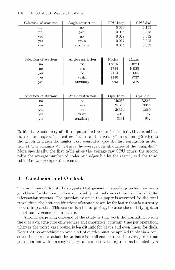
Table 1 presents a summarizing comparison of all combinations of strategies.Note that the total number of algorithmic steps is asymptotically dominated bythe number of operations inside the priority queue. In other words, these opera-tions are representative operation counts in the sense of [4], Sect. 18. More specif-ically, for a heap the number of exchange operations is representative, whereasfor the dial variant the number of cyclic increments of the moving array indexis representative. The average total number per query of these operations arelisted in the last part of Table 1.

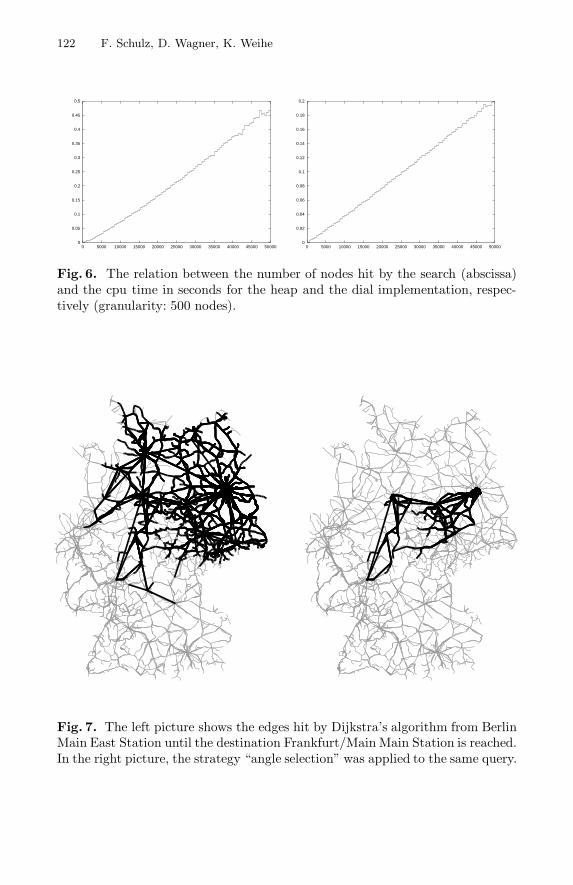
For both implementations of the priority queue, the CPU times imply thesame strong ranking of strategies. Figs. 7 and 8 might give a visual impressionwhy this ranking is so unambiguous. Moreover, the discrepancy between theheap and the dial implementation also decreases roughly from row to row. Thisis not surprising: the overhead of the heap should be positively correlated withthe size of the heap, which is significantly reduced by both strategies.

Our experience with several versions of the code is that the exact CPU timesare strongly sensitive to the details of the implementation, but the general ten-dency is maintained and seems to be reliable. In particular, the main questionraised in this paper (whether optimality–preserving techniques are competitive)can be safely answered in the affirmative at least for the restriction of the prob-lem to the total travel time as the only optimization criterion.

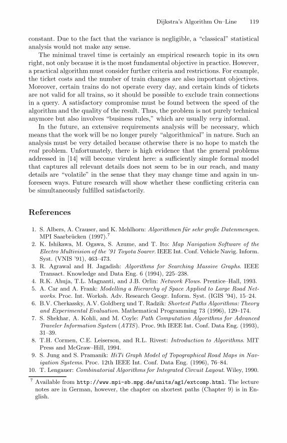
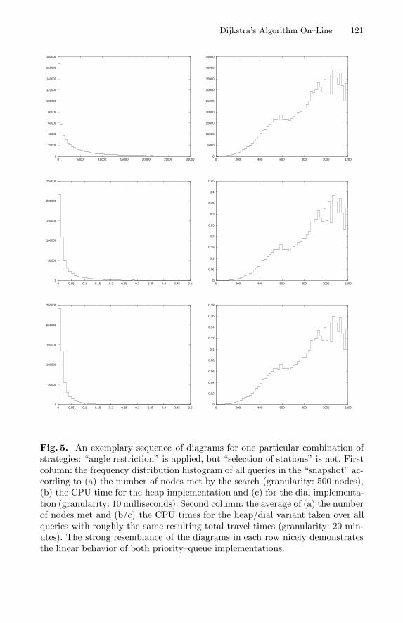
However, a detailed look at the results is more insightful. Fig. 4 showsthat there is a very strong linear correlation between the number of edges hitwith/without strategy “angle restriction.” On the other hand, Fig. 5 shows adetailed analysis of one particular, exemplary combination of strategies. A com-parison of these diagrams reveals an interesting effect, which is also found in theanalogous diagrams of the other combinations: the CPU times of both the heapand the dial implementation are linear in the number of nodes hit by the search.This correlation is so strong and the variance is so small that correspondingdiagrams in Fig. 5 look almost identical. Figure 6 reveals the cause.

In other words, in both cases the operations on the priority queue take con-stant time on average, even when the average is taken over each query separately!This is in great contrast to the asymptotic worst–case complexity of these datastructures.


Selection of stations Angle restriction CPU heap CPU dial

no no 0.310 0.103no yes 0.036 0.018yes no 0.027 0.012yes train 0.007 0.005yes auxiliary 0.005 0.003

Selection of stations Angle restriction Nodes Edges

no no 17576 31820no yes 4744 10026yes no 2114 3684yes train 1140 2737yes auxiliary 993 2378

Selection of stations Angle restriction Ops. heap Ops. dial

no no 246255 23866no yes 24526 3334yes no 26304 3660yes train 4973 1197yes auxiliary 3191 932

Table 1. A summary of all computational results for the individual combina-tions of techniques. The entries “train” and “auxiliary” in column #2 refer tothe graph in which the angles were computed (see the last paragraph in Sec-tion 2). The columns #3–#4 give the average over all queries of the “snapshot.”More specifically, the first table gives the average raw CPU times, the secondtable the average number of nodes and edges hit by the search, and the thirdtable the average operation counts.

4 Conclusion and Outlook

The outcome of this study suggests that geometric speed–up techniques are agood basis for the computation of provably optimal connections in railroad trafficinformation systems. The question raised in this paper is answered for the totaltravel time: the best combinations of strategies are by far faster than is currentlyneeded in practice. This success is a bit surprising, because the underlying datais not purely geometric in nature.

Another surprising outcome of the study is that both the normal heap andthe dial data structure only require an (amortized) constant time per operation,whereas the worst–case bound is logarithmic for heaps and even linear for dials.Note that no amortization over a set of queries must be applied to obtain a con-stant time per operation; the variance is small enough that the average run timeper operation within a single query can essentially be regarded as bounded by a


constant. Due to the fact that the variance is negligible, a “classical” statisticalanalysis would not make any sense.

The minimal travel time is certainly an empirical research topic in its ownright, not only because it is the most fundamental objective in practice. However,a practical algorithm must consider further criteria and restrictions. For example,the ticket costs and the number of train changes are also important objectives.Moreover, certain trains do not operate every day, and certain kinds of ticketsare not valid for all trains, so it should be possible to exclude train connectionsin a query. A satisfactory compromise must be found between the speed of thealgorithm and the quality of the result. Thus, the problem is not purely technicalanymore but also involves “business rules,” which are usually very informal.

In the future, an extensive requirements analysis will be necessary, whichmeans that the work will be no longer purely “algorithmical” in nature. Such ananalysis must be very detailed because otherwise there is no hope to match thereal problem. Unfortunately, there is high evidence that the general problemsaddressed in [14] will become virulent here: a sufficiently simple formal modelthat captures all relevant details does not seem to be in our reach, and manydetails are “volatile” in the sense that they may change time and again in un-foreseen ways. Future research will show whether these conflicting criteria canbe simultaneously fulfilled satisfactorily.

References

1. S. Albers, A. Crauser, and K. Mehlhorn: Algorithmen fur sehr große Datenmengen.MPI Saarbrucken (1997).7

2. K. Ishikawa, M. Ogawa, S. Azume, and T. Ito: Map Navigation Software of theElectro Multivision of the ’91 Toyota Soarer. IEEE Int. Conf. Vehicle Navig. Inform.Syst. (VNIS ’91), 463–473.

3. R. Agrawal and H. Jagadish: Algorithms for Searching Massive Graphs. IEEETransact. Knowledge and Data Eng. 6 (1994), 225–238.

4. R.K. Ahuja, T.L. Magnanti, and J.B. Orlin: Network Flows. Prentice–Hall, 1993.

5. A. Car and A. Frank: Modelling a Hierarchy of Space Applied to Large Road Net-works. Proc. Int. Worksh. Adv. Research Geogr. Inform. Syst. (IGIS ’94), 15–24.

6. B.V. Cherkassky, A.V. Goldberg und T. Radzik: Shortest Paths Algorithms: Theoryand Experimental Evaluation. Mathematical Programming 73 (1996), 129–174.

7. S. Shekhar, A. Kohli, and M. Coyle: Path Computation Algorithms for AdvancedTraveler Information System (ATIS). Proc. 9th IEEE Int. Conf. Data Eng. (1993),31–39.

8. T.H. Cormen, C.E. Leiserson, and R.L. Rivest: Introduction to Algorithms. MITPress and McGraw–Hill, 1994.

9. S. Jung and S. Pramanik: HiTi Graph Model of Topographical Road Maps in Nav-igation Systems. Proc. 12th IEEE Int. Conf. Data Eng. (1996), 76–84.

10. T. Lengauer: Combinatorial Algorithms for Integrated Circuit Layout. Wiley, 1990.

7 Available from http://www.mpi-sb.mpg.de/units/ag1/extcomp.html. The lecturenotes are in German, however, the chapter on shortest paths (Chapter 9) is in En-glish.


11. J. Shapiro, J. Waxman, and D. Nir: Level Graphs and Approximate Shortest PathAlgorithms. Network 22 (1992), 691–717.

12. T. Preuss and J.-H. Syrbe: An Integrated Traffic Information System. Proc. 6thInt. Conf. Appl. Computer Networking in Architecture, Construction, Design, CivilEng., and Urban Planning (europIA ’97).

13. K. Weihe: Reuse of Algorithms — Still a Challenge to Object–Oriented Program-ming. Proc. 12th ACM Symp. Object–Oriented Programming, Systems, Lan-guages, and Applications (OOPSLA ’97), 34–48.

14. K. Weihe, U. Brandes, A. Liebers, M. Muller–Hannemann, D. Wagner, and T.Willhalm: Empirical Design of Geometric Algorithms. To appear in the Proc. 15thACM Symp. Comp. Geometry (SCG ’99).


0

20000

40000

60000

80000

100000

120000

140000

160000

180000

0 5000 10000 15000 20000 25000 300000

5000

10000

15000

20000

25000

30000

35000

40000

45000

0 200 400 600 800 1000 1200

0

50000

100000

150000

200000

250000

0 0.05 0.1 0.15 0.2 0.25 0.3 0.35 0.4 0.45 0.50

0.05

0.1

0.15

0.2

0.25

0.3

0.35

0.4

0.45

0 200 400 600 800 1000 1200

0

50000

100000

150000

200000

250000

0 0.05 0.1 0.15 0.2 0.25 0.3 0.35 0.4 0.45 0.50

0.02

0.04

0.06

0.08

0.1

0.12

0.14

0.16

0.18

0 200 400 600 800 1000 1200

Fig. 5. An exemplary sequence of diagrams for one particular combination ofstrategies: “angle restriction” is applied, but “selection of stations” is not. Firstcolumn: the frequency distribution histogram of all queries in the “snapshot” ac-cording to (a) the number of nodes met by the search (granularity: 500 nodes),(b) the CPU time for the heap implementation and (c) for the dial implementa-tion (granularity: 10 milliseconds). Second column: the average of (a) the numberof nodes met and (b/c) the CPU times for the heap/dial variant taken over allqueries with roughly the same resulting total travel times (granularity: 20 min-utes). The strong resemblance of the diagrams in each row nicely demonstratesthe linear behavior of both priority–queue implementations.


0

0.05

0.1

0.15

0.2

0.25

0.3

0.35

0.4

0.45

0.5

0 5000 10000 15000 20000 25000 30000 35000 40000 45000 500000

0.02

0.04

0.06

0.08

0.1

0.12

0.14

0.16

0.18

0.2

0 5000 10000 15000 20000 25000 30000 35000 40000 45000 50000

Fig. 6. The relation between the number of nodes hit by the search (abscissa)and the cpu time in seconds for the heap and the dial implementation, respec-tively (granularity: 500 nodes).

Fig. 7. The left picture shows the edges hit by Dijkstra’s algorithm from BerlinMain East Station until the destination Frankfurt/Main Main Station is reached.In the right picture, the strategy “angle selection” was applied to the same query.


Fig. 8. The first picture shows the 225 stations selected for the study on strategy“selection of stations.” The remaining three pictures refer to the same query asin Fig. 7. However, now the strategy “selection of stations” is applied with noangle restriction (upper right), with angles computed from the train graph (lowerleft), and with angles computed from the auxiliary graph itself. The train graphis shown in the background. The highlighted edges are the edges of the auxiliarygraph hit by the search.

dijkstra's algorithm on–line: an empirical case study from public

Documents