digital soil mapping of key soil properties over new …...digital soil mapping of key soil...

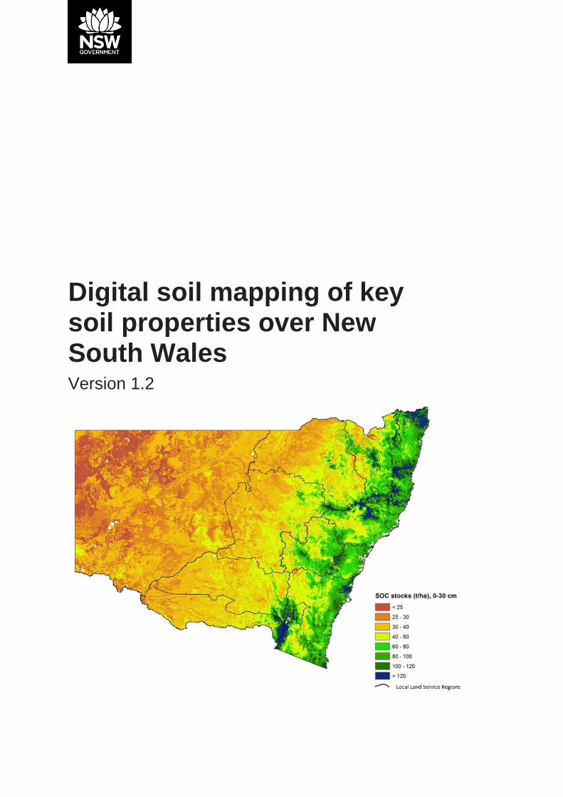
Digital soil mapping of key soil properties over New South Wales Version 1.2

© 2018 State of NSW and Office of Environment and Heritage With the exception of photographs, the State of NSW and Office of Environment and Heritage are pleased to allow this material to be reproduced in whole or in part for educational and non-commercial use, provided the meaning is unchanged and its source, publisher and authorship are acknowledged. Specific permission is required for the reproduction of photographs. The Office of Environment and Heritage (OEH) has compiled this report in good faith, exercising all due care and attention. No representation is made about the accuracy, completeness or suitability of the information in this publication for any particular purpose. OEH shall not be liable for any damage which may occur to any person or organisation taking action or not on the basis of this publication. Readers should seek appropriate advice when applying the information to their specific needs. All content in this publication is owned by OEH and is protected by Crown Copyright, unless credited otherwise. It is licensed under the Creative Commons Attribution 4.0 International (CC BY 4.0), subject to the exemptions contained in the licence. The legal code for the licence is available at Creative Commons. OEH asserts the right to be attributed as author of the original material in the following manner: © State of New South Wales and Office of Environment and Heritage 2018. Front cover: Digital soil map of soil organic carbon stocks (0-30 cm) over New South Wales (J. Gray/OEH). This report was prepared by Jonathan Gray, in conjunction with other staff from the Evaluation and Assessment Teams of Ecosystem Management Science Branch, Science Division, NSW Office of Environment and Heritage. Thomas Bishop (University of Sydney) and Senani Karunaratne (Australian Department of Environment) provided useful assistance and advice.

Published by: Office of Environment and Heritage 59 Goulburn Street, Sydney NSW 2000 PO Box A290, Sydney South NSW 1232 Phone: +61 2 9995 5000 (switchboard) Phone: 1300 361 967 (OEH and national parks enquiries) TTY users: phone 133 677, then ask for 1300 361 967 Speak and listen users: phone 1300 555 727, then ask for 1300 361 967 Email: [email protected] Website: www.environment.nsw.gov.au Report pollution and environmental incidents Environment Line: 131 555 (NSW only) or [email protected] See also www.environment.nsw.gov.au ISBN 978-1-925754-59-9 OEH 2018/ 0489 November 2018

Find out more about your environment at:

www.environment.nsw.gov.au

http://creativecommons.org/licenses/by/4.0/deed.en

http://creativecommons.org/licenses/by/4.0/deed.en

http://creativecommons.org/licenses/by/4.0/legalcode

mailto:[email protected]

http://www.environment.nsw.gov.au/

mailto:[email protected]

http://www.environment.nsw.gov.au/

iii

Contents Abbreviations and acronyms v

Summary 1

1. Introduction 2

1.1 Existing digital soil mapping over New South Wales 2 1.2 Aims 3

2. Methods 4

2.1 Overview 4 2.2 Soil data 4 2.3 Covariates 7 2.4 Modelling approach 8 2.5 Map production 9 2.6 Validation 9

3. The digital soil maps 10

3.1 The maps 10 3.2 Map validation 23

4. Discussion 26

4.1 Strategy for use 26 4.2 Limitations 26 4.3 Relation to existing DSM and conventional soil survey products 27 4.4 Conclusion 28

Appendix 1: Covariate layers 29

Appendix 2: Multiple linear regression models 34

References 38

iv

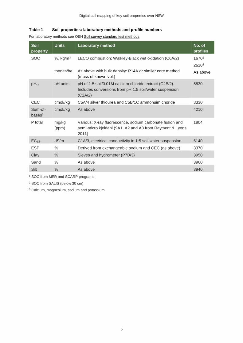
List of tables Table 1 Soil properties: laboratory methods and profile numbers 5

Table 2 Digital soil map validation results 23

List of figures Figure 1 Overview of the digital soil mapping process 6

Figure 2 Soil organic carbon (SOC) concentration (%) 11 Figure 3 Soil organic carbon (SOC) mass (kg/m3) 12

Figure 4 Soil organic carbon (SOC) stocks (tonnes/ha) 13

Figure 5 pH (CaCl2) 14 Figure 6 Cation exchange capacity (CEC) 15

Figure 7 Sum-of-bases 16

Figure 8 Total phosphorous 17 Figure 9 Electrical conductivity (EC1:5) 18

Figure 10 Exchangeable sodium percent (ESP) 19

Figure 11 Clay 20 Figure 12 Sand 21

Figure 13 Silt 22

Digital soil mapping of key soil properties over NSW

v

Abbreviations and acronyms SCARP Australian Soil Carbon Research Program CEC cation exchange capacity DEM digital elevation model DSM digital soil maps EC electrical conductivity ESP exchangeable sodium percent GIS geographical information system P phosphorous MER monitoring, evaluation and reporting MLR multiple linear regression RMSE root mean square error SALIS Soil and Land Information System SLGA Soil and Landscape Grid of Australia SOC soil organic carbon


vi


1

Summary The Office of Environment and Heritage (OEH) has prepared digital soil maps (DSMs) for a range of key soil properties over New South Wales. These are maps derived through quantitative modelling techniques that are based on relationships between soil attributes and the environment. DSMs are presented for soil organic carbon (SOC), pH, cation exchange capacity, sum-of-bases, total phosphorous, electrical conductivity (EC), exchangeable sodium percent (ESP), clay, sand and silt. The maps are at 100-m spatial resolution and cover six soil depth intervals down to two metres, consistent with major Australian and international systems. The modelling techniques applied included multiple linear regression and Cubist decision-tree approaches. Validation results for the maps indicate variable performance and effectiveness, with Lin’s concordance values approaching 0.8 for pH and sum-of-bases at deeper levels, but dropping below 0.20 for ESP and SOC at deeper levels. The maps provide at least a useful first approximation of these soil properties across the State. They may be viewed directly through the OEH spatial viewer eSPADE and are also available for download as geographical information system (GIS) or PDF files through the NSW Government environmental data portal SEED. These DSMs represent an alternative and complementary product to the Australia-wide DSMs presented within the Soil and Landscape Grid of Australia, being based on NSW rather than nation-wide data, and including several different soil properties. These new maps also complement existing conventional soil landscape products available for much of New South Wales. Together with the existing maps, the new DSMs help inform on vital soil conditions throughout the State and assist in the ongoing sustainable management and protection of these important resources. They also provide valuable input data for a range of other natural resource and environmental modelling systems throughout the State.

http://espade.environment.nsw.gov.au/

https://datasets.seed.nsw.gov.au/dataset/digital-soil-maps-for-key-soil-properties-over-nsw


2

1. Introduction Digital soil mapping (DSM) has become established over the last two decades as an important avenue for collecting important soil information. DSMs are prepared through quantitative modelling techniques based on relationships between soil properties or classes and the environment. The underlying models have their roots in the fundamental soil equation of Dokuchaev (1899) and Jenny (1941): s = f(cl, o, r, p, t, … ), which states that soils are a function of climate, organisms, relief, parent material and time. More recently, this conceptual model has been further advanced with the ‘s, c, o, r, p, a, n’ approach of McBratney et al. (2003), which has the additional factors of s (a soil attribute predictor) and n (a geographic position predictor) and also incorporates modelling of residual errors. The DSM approach uses available environmental data to represent each of these soil-influencing factors, developing the relationships over known soil data points then extrapolating these relationships over broad regions using continuous environmental data grids (e.g. climate grids, digital elevation models or gamma radiometric data grids). DSMs have the potential to be a valuable complement to existing, conventional soil landscape mapping products over New South Wales. They can:

• provide estimates of specific soil properties or classes down to fine grid size (e.g. 100-m pixels), rather than broad polygons

• provide coverage for soil data for areas of the State with nil or only very broadscale existing soil data

• provide estimates for soil properties that may not have been included in original soil surveys and laboratory analyses

• provide data in a spatial format more readily applied by quantitative environmental modellers, e.g. ecological, hydrological and climate change modellers.

However, conventional soil maps do retain many advantages over digital soil maps, including their more holistic approach in describing soil character, and the two mapping forms are best applied together. Further discussion on the relation of DSM to conventional soil mapping is given in Discussion (Section 4.3).

1.1 Existing digital soil mapping over New South Wales Regional and broader scale DSMs have been undertaken over New South Wales in a number of projects during the past decade. A recent major national project has resulted in the release of the Soil and Landscape Grid of Australia (SLGA) (Grundy et al. 2015; Viscarra Rossel et al. 2015). This includes DSMs for a wide range of key soil properties over the entire Australian continent at three arc second grid (approximately 90m), with six depth intervals down to two metres. Associated maps presenting upper and lower 95% confidence level predictions are also provided. This product represents Australia’s contribution to a proposed global digital soil map: GlobalSoilMap.net (Sanchez et al. 2009; Arrouays et al. 2014). Prior to this, digital mapping over Australia’s agricultural zone had been carried out for a range of soil properties including pH, SOC, total phosphorous (P) and clay over topsoils and subsoils by Henderson et al. (2005) at 250-m resolution. Soil carbon was further digitally mapped across most or all of the country by Bui et al. (2009), Viscarra Rossel et al. (2014) and Gray et al. (2015a). Local catchment and field-scale DSMs have been carried out within New South Wales for various soil properties, for example by Minasny et al. (2006); Malone et al. (2009); Triantafilis et al. (2009) and Karunaratne et al. (2014).

http://www.csiro.au/soil-and-landscape-grid


3

1.2 Aims The above broadscale digital soil map products were developed using soil data from all over Australia. In this current project, DSMs are prepared using only NSW soil data (except for P total which used data from all eastern Australia). The environmental data (i.e. covariate layers) also covered New South Wales only. These new maps should provide further modelled evidence of soil properties across New South Wales that can be compared to and complement the existing continental-scale DSMs and also the NSW conventional soil maps. This project aims to:

• use multiple linear regression (MLR) and Cubist decision-tree modelling techniques to prepare DSMs over New South Wales, covering the key soil properties of SOC, pH, cation exchange capacity (CEC), sum-of-bases, total P, electrical conductivity (EC1:5), ESP, clay, sand and silt

• use 100-m resolution raster over six depth intervals down to 2m, consistent with the SLGA and GlobalSoilMap.net

• provide validation results for the models and maps • discuss interpretation and use of the maps. The subject soil properties are essential for effective agricultural, hydrological, climatic, ecological and other scientific studies. The properties of SOC, pHca, CEC, sum-of-bases, total P, EC and ESP are indicators of a soil’s chemical condition, its nutrient status and potential to retain nutrients. The clay, silt and sand content of a soil control its texture and physical behaviour, including water holding capacity and permeability, and also influence many chemical characteristics. The storage of carbon in soil is considered vital in addressing global climate change (Baldock et al. 2012).


4

2. Methods

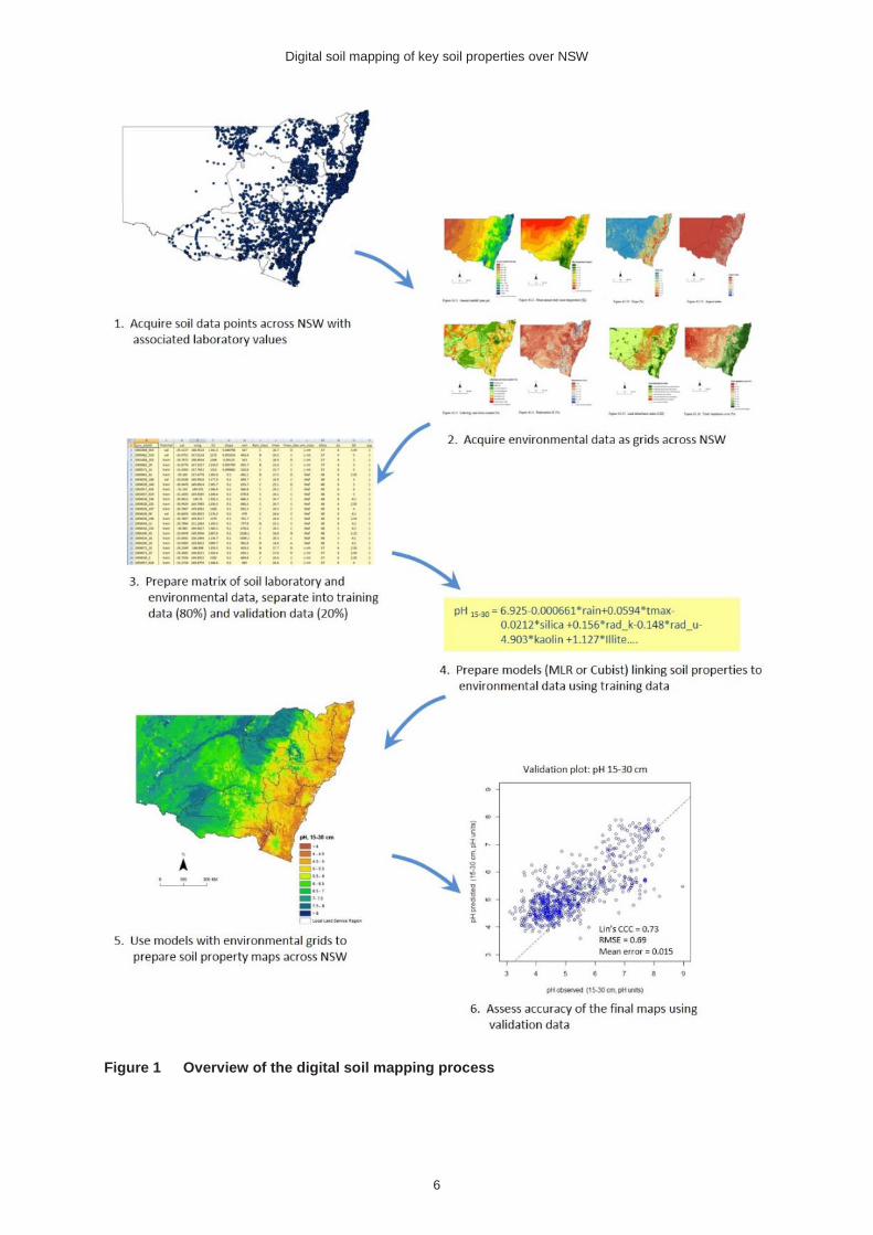
2.1 Overview The digital soil maps (DSM) of the ten soil properties were prepared at six depth intervals down to two metres. They were based on soil survey data available over New South Wales, except for total P which used data from all over eastern Australia. These data were divided into training and validation subsets, at an approximate 80:20% ratio. Environmental covariate data representing the main soil-forming factors were applied in the initial training models and final maps production. These were derived from field survey data and various environmental data grids covering the entire State. The modelling approach was predominantly multiple linear regression, but the Cubist decision-tree approach was applied for some of the soil properties. Validation of the initial models and then the final digital soil maps was carried out using the validation dataset. Figure 1 presents a simple flowchart of the DSM process applied in this project.

2.2 Soil data Soil data for most soil properties was derived from the NSW Soil and Land Information System (SALIS). An exception was for soil organic carbon (SOC) upper 30-cm layers that used data from the 2008 NSW monitoring, evaluation and reporting (MER) program (Chapman et al. 2011; OEH 2014) and the Australian Soil Carbon Research Program (SCARP) (Sanderman et al. 2011), because of the stronger modelling performance and availability of bulk density measurements (allowing for estimates of SOC stocks). Another exception was for total P, which was not available in SALIS, so data was derived from all eastern State natural resource agencies, as described in Gray et al. (2015b). Only profiles with full laboratory data and meaningful parent material descriptions were applied. Final profile numbers, plus the laboratory analytical method, are listed in Table 1. The soil dataset was randomly apportioned 80% as training data and 20% as validation data.

http://www.environment.nsw.gov.au/soils/data.htm

http://www.environment.nsw.gov.au/soils/data.htm

http://doi.org/10.4225/08/5101F31440A36


5

Table 1 Soil properties: laboratory methods and profile numbers For laboratory methods see OEH Soil survey standard test methods.

Soil property

Units Laboratory method No. of profiles

SOC %, kg/m3

tonnes/ha

LECO combustion; Walkley-Black wet oxidation (C6A/2)

As above with bulk density: P14A or similar core method (mass of known vol.)

16701

26102

As above

pHca pH units pH of 1:5 soil/0.01M calcium chloride extract (C2B/2). Includes conversions from pH 1:5 soil/water suspension (C2A/2)

5830

CEC cmolc/kg C5A/4 silver thiourea and C5B/1C ammonuim choride 3330

Sum-of-bases3

cmolc/kg As above 4210

P total mg/kg (ppm)

Various: X-ray fluorescence, sodium carbonate fusion and semi-micro kjeldahl (9A1, A2 and A3 from Rayment & Lyons 2011)

1804

EC1:5 dS/m C1A/3, electrical conductivity in 1:5 soil:water suspension 6140

ESP % Derived from exchangeable sodium and CEC (as above) 3370

Clay % Sieves and hydrometer (P7B/3) 3950

Sand % As above 3960

Silt % As above 3940 1 SOC from MER and SCARP programs 2 SOC from SALIS (below 30 cm) 3 Calcium, magnesium, sodium and potassium

http://www.environment.nsw.gov.au/soils/testmethods.htm


6

Figure 1 Overview of the digital soil mapping process


7

In addition to SOC concentration (%), SOC mass (kg/m3) was also derived by applying bulk density estimates included within the MER and SCARP datasets down to 30cm, and derived from the SLGA below 30cm. Stocks of SOC (tonnes/ha) were also calculated directly from the mass estimates in the final digital soil maps, but only over two intervals: 0–30cm and 30–100cm. To avoid reporting two separate pH test results, pHw values were converted into pHca values using the correlation tables of Henderson and Bui (2002). The latter mode is preferred in Australia as it more closely represents the ionic soil solutions typically found in the field, and thus gives more consistent results. The soil datasets were organised into six depth intervals down to 2m, that is, 0–5, 5–15, 15–30, 30–60, 60–100 and 100–200cm. These depth intervals were selected to be consistent with the SLGA and the global digital soil mapping project GlobalSoil.Net. Soil property values reported for the original depth interval of each soil horizon were converted into these standard depth intervals using the equal area splining process of Bishop et al. (1999) and Malone et al. (2009).

2.3 Covariates Covariates were selected to effectively represent each of the key soil-forming factors of climate, parent material, relief, biota and age, as outlined below. Further detail is provided in the cited references.

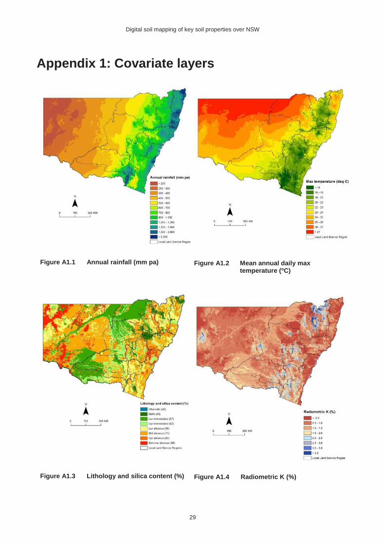
Climate 1. Mean annual rainfall (mm pa, rain) derived from 2.5-km Australia-wide climate grids

from the Australian Bureau of Meteorology with resampling of cell values down to a 100-m grid. The values represent mean values obtained over the 1961–90 period, which overlaps or slightly predates the period when most of the soil profiles were collected (see Appendix 1, Figure A1.1)

2. Mean annual daily maximum temperature (oC, Tmax) – as above (see Appendix 1, Figure A1.2)

Parent material 1. Lithology – the basis of this covariate was the lithology of the parent material, and more

specifically the silica content (%) which is applied as a silica index. Silica content provides a simple but meaningful quantitative estimate of the chemical composition of most parent materials. It generally has a direct relationship to quartz content and an inverse relationship with basic cation content (Gray et al. 2016). For example, granite is moderately siliceous with approximately 73% silica, while basalt is mafic material with only approximately 48% silica. Higher silica content parent materials typically give rise to soils with more quartzose sandier textures with lower chemical fertility. For model development, the description of parent material or geologic unit recorded at each site by the soil surveyor was used. For the final map preparation, lithological classes and silica index values were applied manually to each geological formation as identified in the 1:250 000-scale digital geology map of the Geological Survey of NSW (NSW Department of Resources and Energy, undated). For poorly defined Cainozoic unconsolidated material, such as unqualified ‘alluvium’ or ‘colluvium’ for which their broad composition is unknown, lithological classes were allocated following reference to existing soil type maps. This exploited clear soil type to parent material relationships, such as Black Vertosols (Isbell 2002) with the mafic class and highly sandy Tenosols or Rudosols with the upper siliceous class. Note that calcareous and some other lithology types could not be characterised in any meaningful way by their silica content. These


8

occupy small areas across New South Wales and generally occur as minor components of broader mixed geology units (see Appendix 1, Figure A1.3).

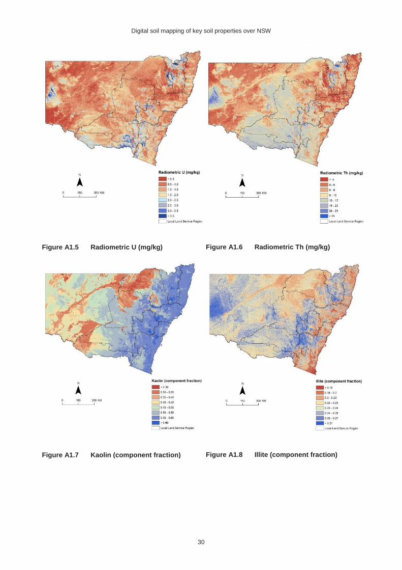
2. Gamma radiometrics – radiometric potassium (rad_K), uranium (rad_U) and thorium (rad_Th); 90-m grids developed by and sourced from Geoscience Australia (see Appendix 1, Figure A1.4–6).

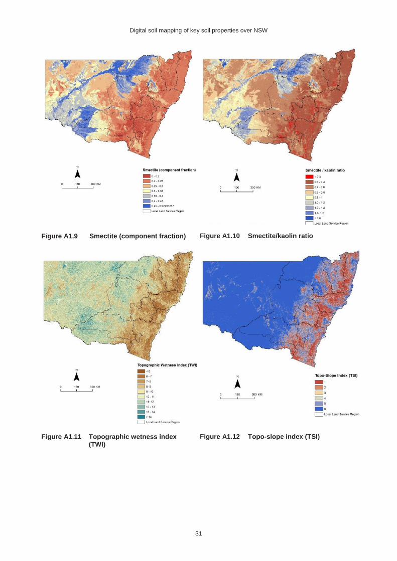
3. NIR clay components – the relative proportions of kaolin, illite and smectite clays and the smectite/kaolin ratio (S/K_ratio) derived from DSM techniques based on laboratory near infra-red (NIR) spectroscopy (Viscarra Rossel 2011); 90-m grids sourced through the CSIRO Data Access Portal via the SLGA (see Appendix 1, Figure A1.7–10).

Relief 1. Topographic wetness index (TWI) – a widely used index that represents potential

hydrological conditions based on slope and catchment area, as derived from digital elevation models (DEMs) (Gallant & Austin 2015); sourced through the CSIRO Data Access Portal via the SLGA (see Appendix 1, Figure A1.11).

2. Topo-slope index (TSI) – an index that combines topographic position and slope gradient, representing the degree to which a site is subject to depletion (1) or accumulation (6) of water, soil particles and chemical materials. Data was derived from field data and a 100-m DEM (Gray et al. 2015b) (see Appendix 1, Figure A1.12).

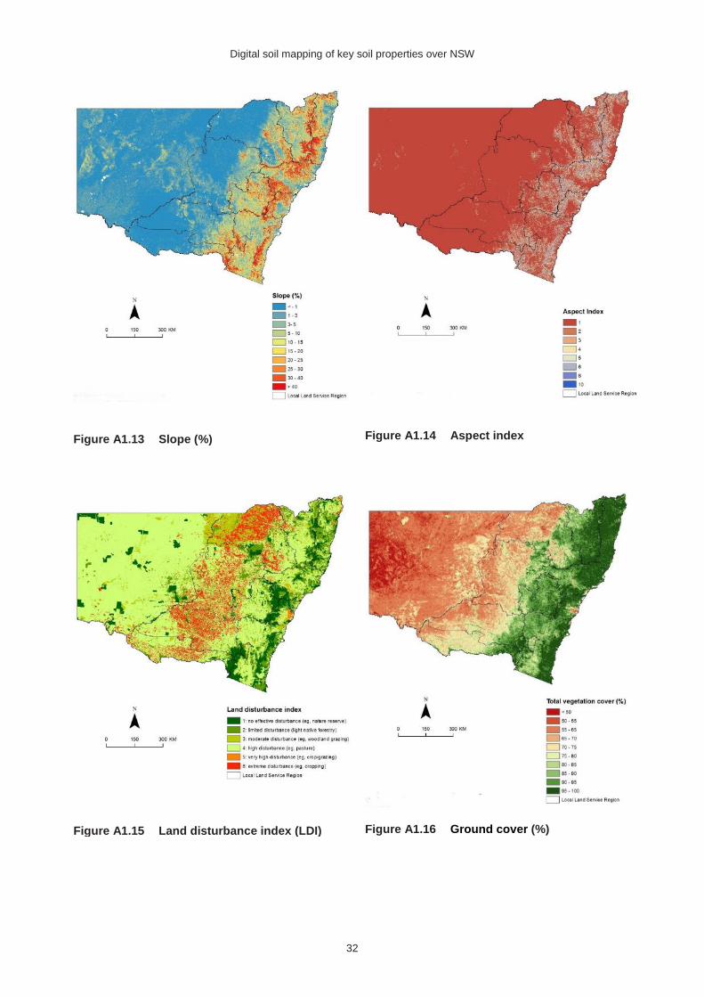
3. Slope – slope gradient in percent as derived from a 100-m DEM (see Appendix 1, Figure A1.13).

4. Aspect index (Asp) – an index to represent the amount of solar radiation received by sites, ranging from 1 for flat areas and gentle north or north-west facing slopes (high radiation in southern hemisphere) to 10 for steep south and south-east facing slopes (low radiation) (Gray et al. 2015b) (see Appendix 1, Figure A1.14).

Biota 1. Land disturbance index (LDI) – an index that reflects the intensity of disturbance

associated with the land use (Gray et al. 2015b), where 1 denotes natural ecosystems and 6 denotes intensive cropping, based on 1:25 000-scale land-use mapping (OEH 2007) (see Appendix 1, Figure A1.15)

2. Ground cover (Ground_cov) – total vegetation cover % (photo-synthetic and non-photo-synthetic) derived from CSIRO, 2011 MODIS fractional vegetation data (Guerschman et al. 2009) (see Appendix 1, Figure A1.16).

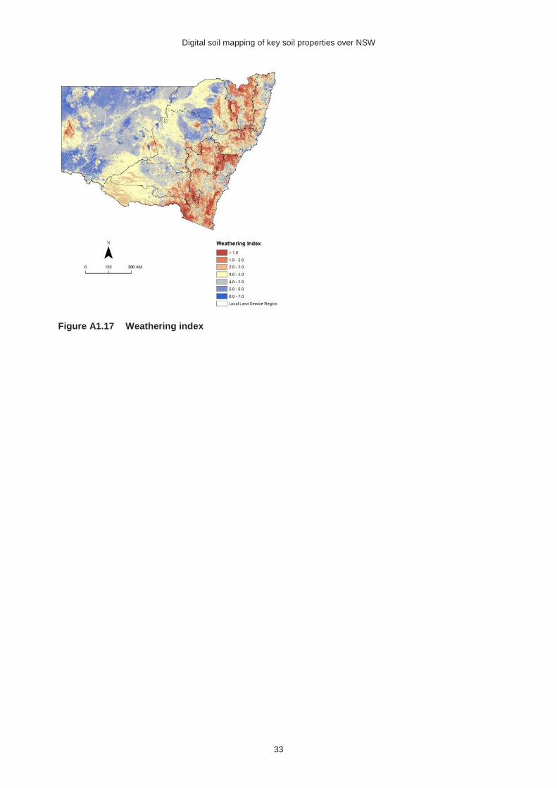
Age Weathering index (W_I) – an index to represent the degree of weathering of parent materials, regolith and soil, based on gamma radiometric data (Wilford 2012); 90-m grids were sourced from Geoscience Australia. The index is considered reflective of the age factor in the clorpt and scorpan frameworks (see Appendix 1, Figure A1.17).

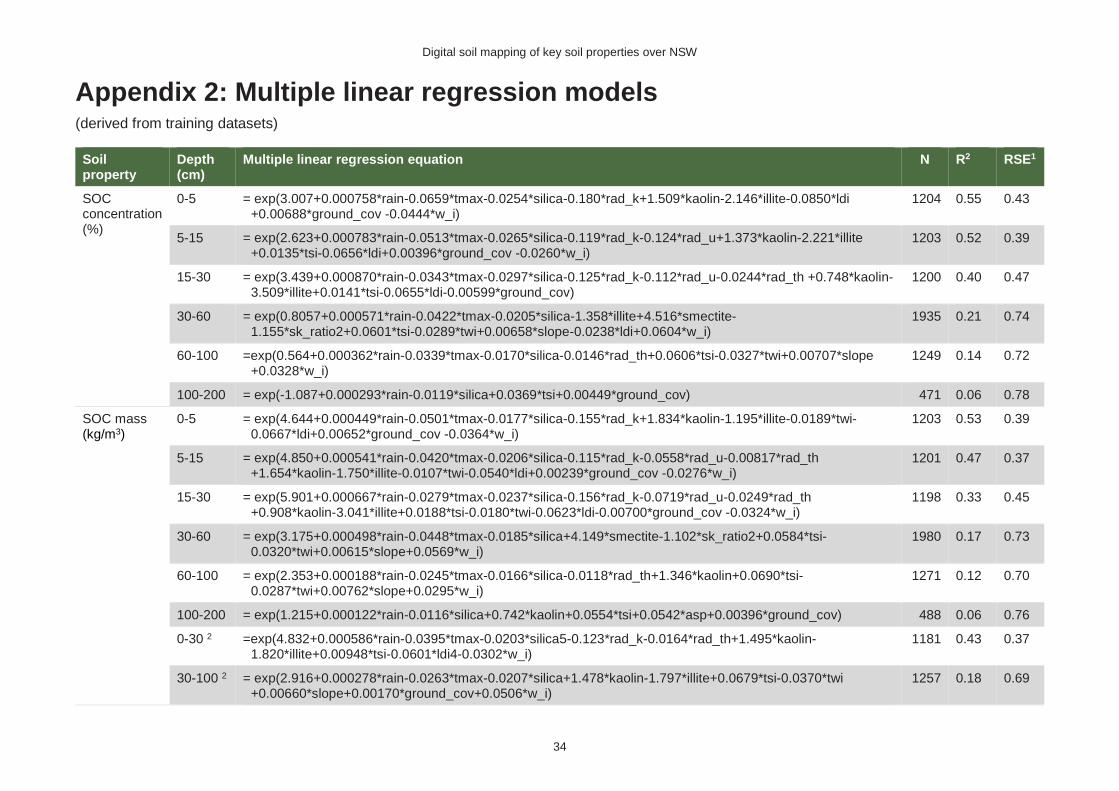
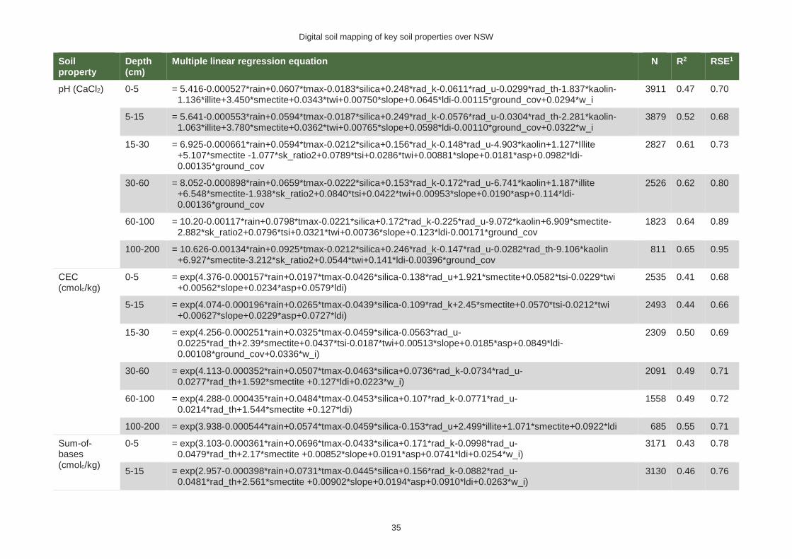
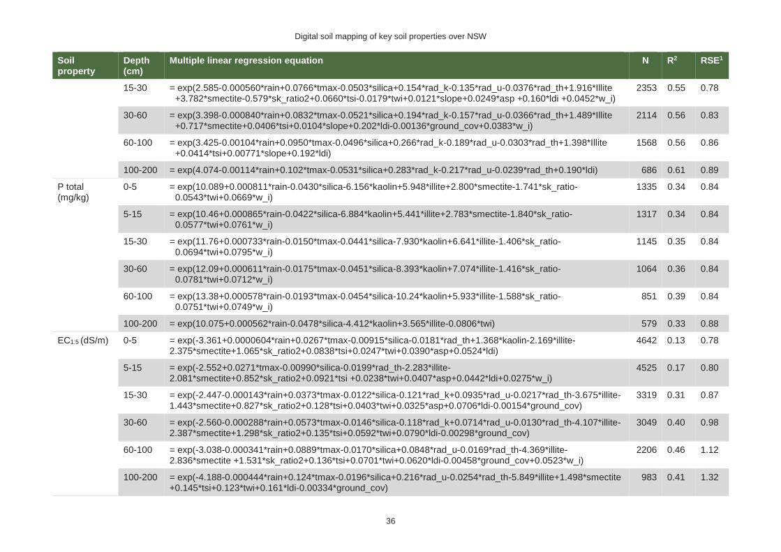
2.4 Modelling approach Most of the digital soil maps were developed using multiple linear regression (MLR) models. A full listing of these models for each soil property and depth interval is provided in Appendix 2, together with sample numbers, coefficient of determination (R2) values and residual standard errors. An example of an MLR model prepared for SOC is shown below:

SOC5_15 = exp(2.623+0.000783*rain-0.0513*tmax-0.0265*silica-0.119*rad_k-0.124*rad_u +1.373*kaolin-2.221*illite +0.0135*tsi-0.0656*ldi+0.00396*ground_cov -0.0260*w_i)


9

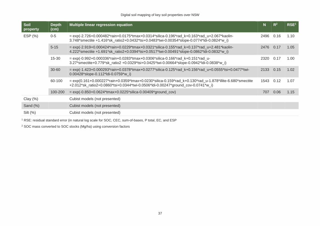
However, for clay, sand and silt, Cubist linear piecewise decision-tree models (Quinlan 1992) were applied. An example extract (showing two of the six rules) for the sand % (15–30 cm) model is shown below:

Rule 1:

If: silica <= 57

then: outcome = 84.77 - 70 smectite - 2.8 ldi - 0.21 ground_cov - 28 kaolin + 2.5 rad_u + 0.1 silica - 0.06 rad_th

Rule 2:

If: silica > 57; silica <= 69: slope > 1.72715: w_i <= 5.0361

then: outcome = -135.83 + 3.09 silica - 0.0159 rain - 4.2 sk_ratio + 0.5 rad_k - 0.02 slope + 0.1 twi

The MLR approach was found to produce more consistent maps with less anomalies and edge effects than the Cubist approach for most soil properties. It also has an advantage of being more ‘transparent’ and readily interpreted, particularly by non-DSM experts (see Gray et al. 2015b). Analysis was carried out using R statistical software (R Core Team 2013). The Cubist approach applied the package of Kuhn et al. (2014). A natural log transformation was applied to several of the soil properties (SOC, CEC, sum-of-bases, total P) to address the observed skewness in the response.

2.5 Map production Final maps were generated using ESRI ArcGIS software together with the above models. For those properties using the MLR models, these were run through the raster calculator tool by applying the equations (shown in Appendix 2) together with estimated values from the respective environmental covariate grids. For those properties using the Cubist models, these were run through a special tool for ArcGIS developed by Reuter (2011). The kriging of residual errors was trialled in order to incorporate any consistent spatial patterns of modelling error (Odeh 1995), but was not adopted in the final maps due to persistent anomalies. Additional maps at 0-30 centimetres and 30-100 centimetres depth intervals were also prepared by combining the component layers, using weighted averages, through the GIS.

2.6 Validation The initial models and final digital soil maps were validated using the validation datasets (approximately 20% of original data points). Lin’s concordance correlation coefficient was used to measure the level of agreement of predicted values with observed values, relative to the 1:1 line (Lin 1989). Also determined were root mean square error (RMSE) and mean error. Preliminary maps of first-approximation, upper and lower 90% confidence limits for each soil property and depth layer were derived by using the RMSE values. For 90% confidence limits, the upper and lower estimates were derived by adding or subtracting 1.645 x RMSE (applying natural log scales where necessary). The adoption of more sophisticated techniques such as the cross-validation techniques demonstrated by Malone et al. (2014) and Kidd et al. (2015) should reduce the high uncertainty levels demonstrated by this first approximation validation process. The collection of independent validation data using a design-based sampling approach would also improve the assessment of accuracy and quality of the maps (Brus et al. 2011).


10

3. The digital soil maps Most of the models that were used to derive the maps for each of the soil properties are presented in Appendix 1, together with the associated validation results.

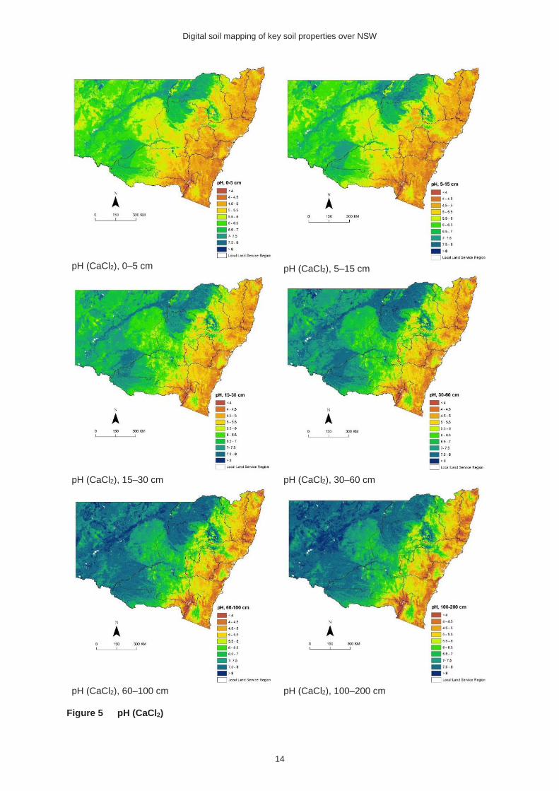
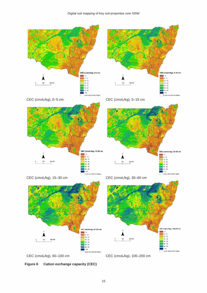
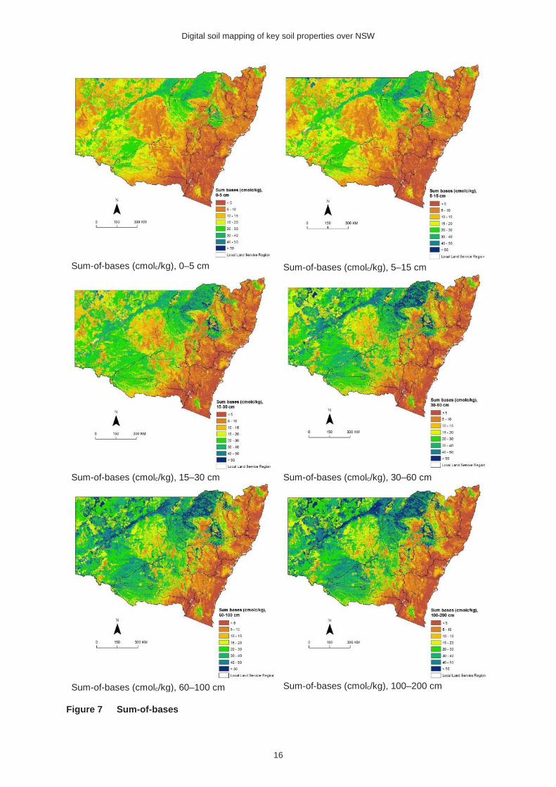
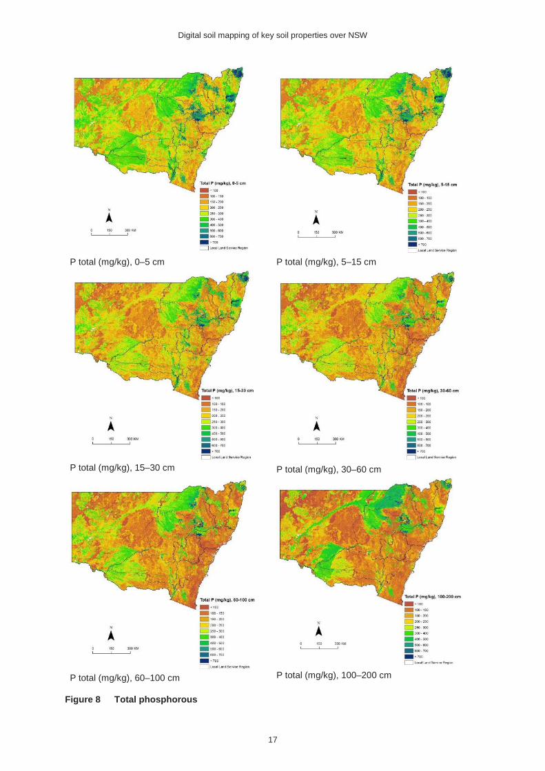
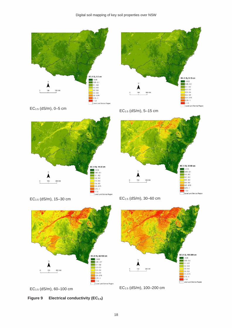
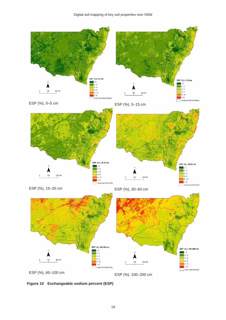
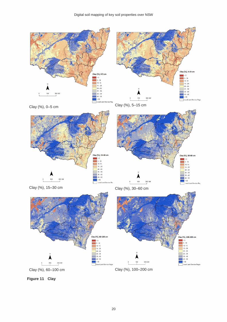
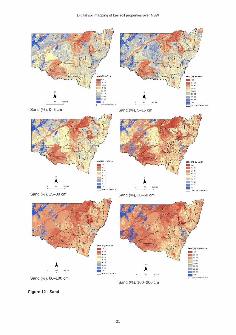
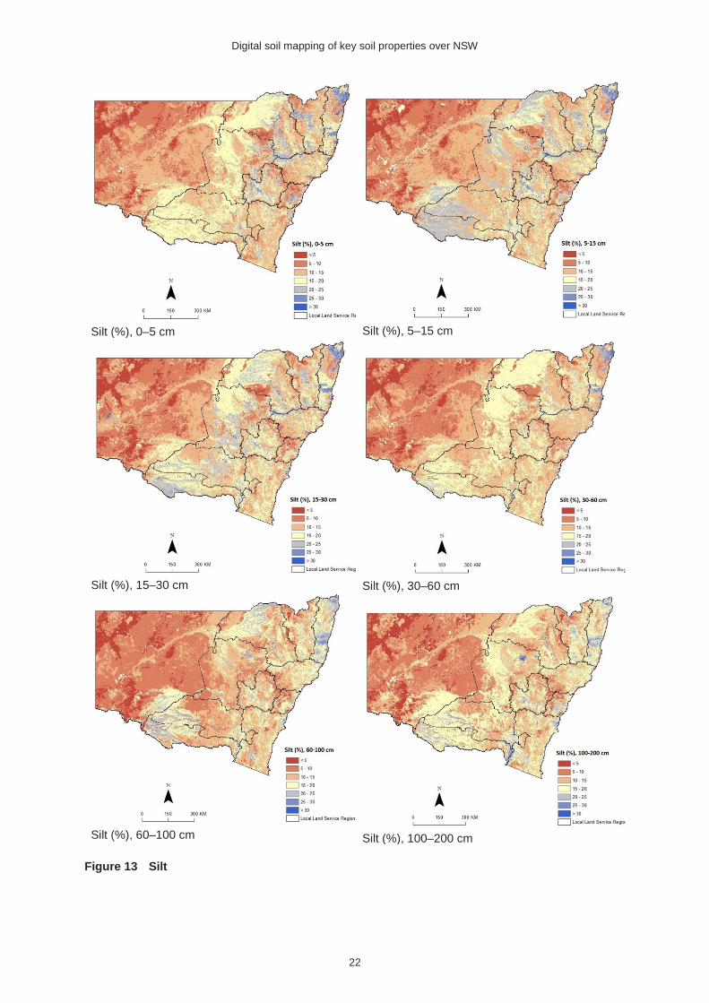
3.1 The maps The maps for the six layers for each soil property are presented in Figures 2 to 13 below. They are presented in terms of classes (e.g. SOC <1%, 1–2%, etc.). Validation statistics for the maps are presented in Table 2 and discussed at the end of the section.


11

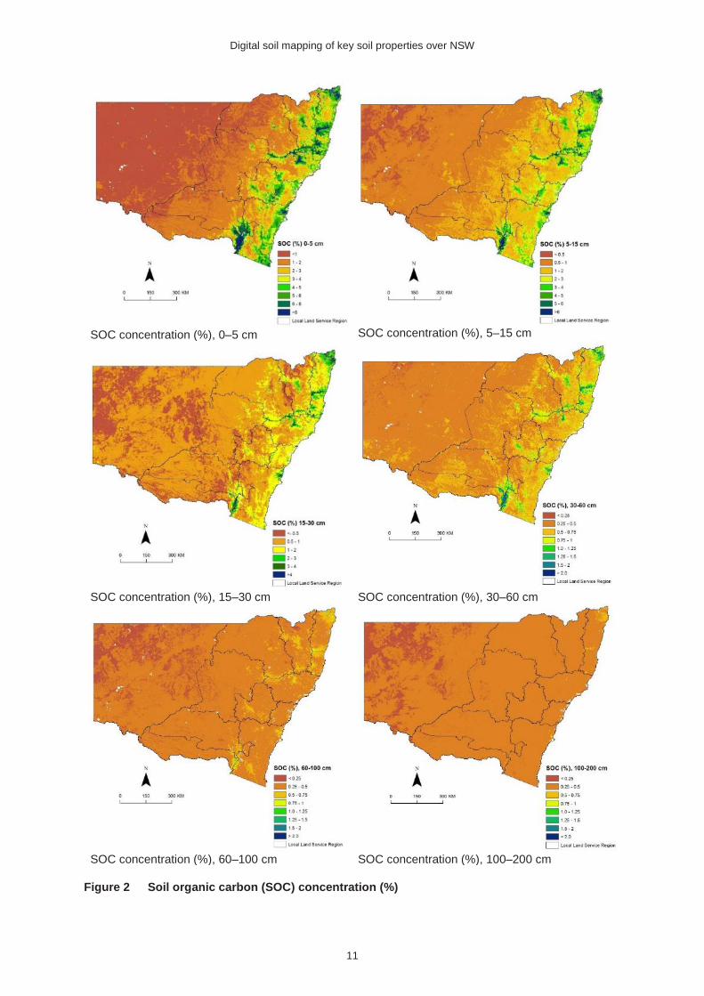
SOC concentration (%), 0–5 cm






Figure 2 Soil organic carbon (SOC) concentration (%)


12

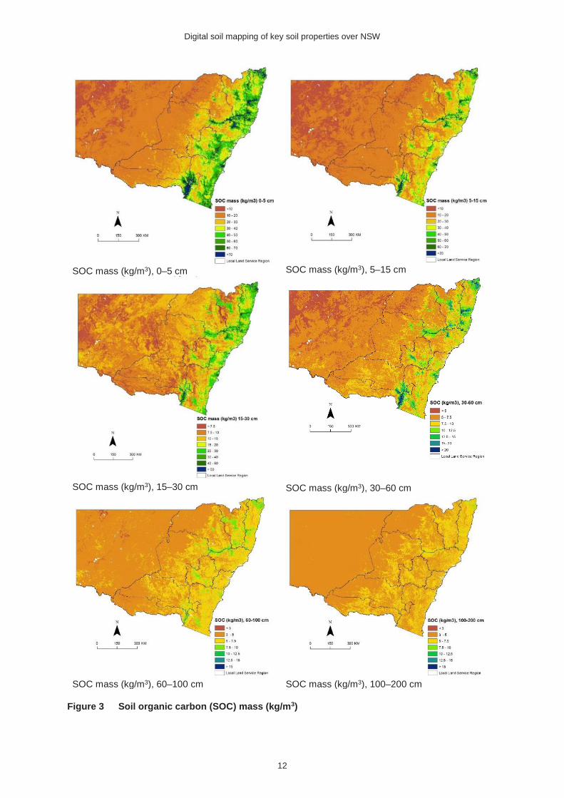
SOC mass (kg/m3), 0–5 cm






Figure 3 Soil organic carbon (SOC) mass (kg/m3)


13

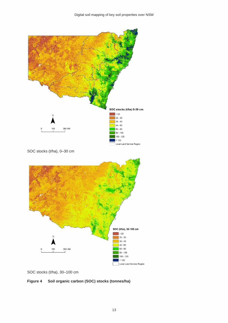
SOC stocks (t/ha), 0–30 cm

SOC stocks (t/ha), 30–100 cm

Figure 4 Soil organic carbon (SOC) stocks (tonnes/ha)


14

pH (CaCl2), 0–5 cm




pH (CaCl2), 60–100 cm

pH (CaCl2), 100–200 cm

Figure 5 pH (CaCl2)


15

CEC (cmolc/kg), 0–5 cm






Figure 6 Cation exchange capacity (CEC)


16

Sum-of-bases (cmolc/kg), 0–5 cm






Figure 7 Sum-of-bases


17

P total (mg/kg), 0–5 cm






Figure 8 Total phosphorous


18

EC1:5 (dS/m), 0–5 cm

EC1:5 (dS/m), 5–15 cm

EC1:5 (dS/m), 15–30 cm

EC1:5 (dS/m), 30–60 cm

EC1:5 (dS/m), 60–100 cm

EC1:5 (dS/m), 100–200 cm

Figure 9 Electrical conductivity (EC1:5)


19

ESP (%), 0–5 cm

ESP (%), 5–15 cm

ESP (%), 15–30 cm

ESP (%), 30–60 cm

ESP (%), 60–100 cm

ESP (%), 100–200 cm

Figure 10 Exchangeable sodium percent (ESP)


20

Clay (%), 0–5 cm

Clay (%), 5–15 cm

Clay (%), 15–30 cm

Clay (%), 30–60 cm

Clay (%), 60–100 cm

Clay (%), 100–200 cm

Figure 11 Clay


21

Sand (%), 0–5 cm

Sand (%), 5–15 cm

Sand (%), 15–30 cm

Sand (%), 30–60 cm

Sand (%), 60–100 cm

Sand (%), 100–200 cm

Figure 12 Sand


22

Silt (%), 0–5 cm

Silt (%), 5–15 cm

Silt (%), 15–30 cm

Silt (%), 30–60 cm

Silt (%), 60–100 cm

Silt (%), 100–200 cm

Figure 13 Silt


23

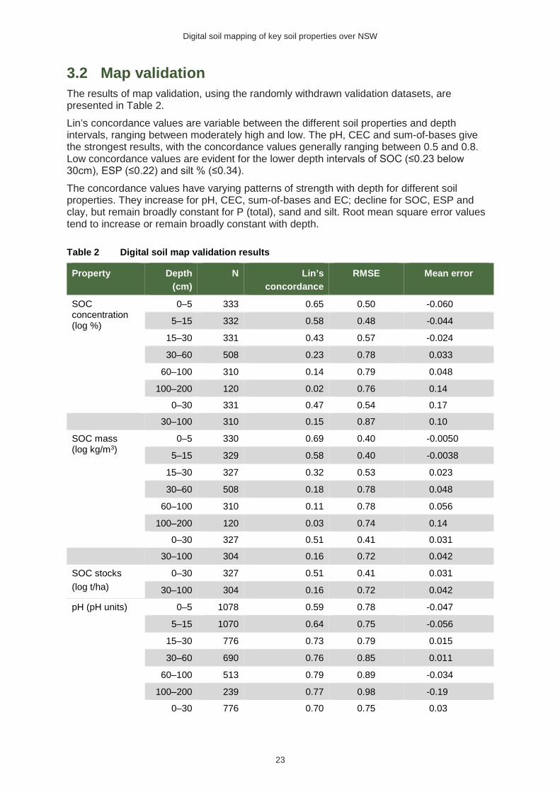
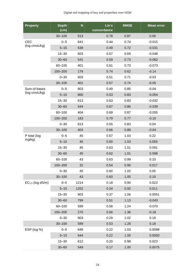
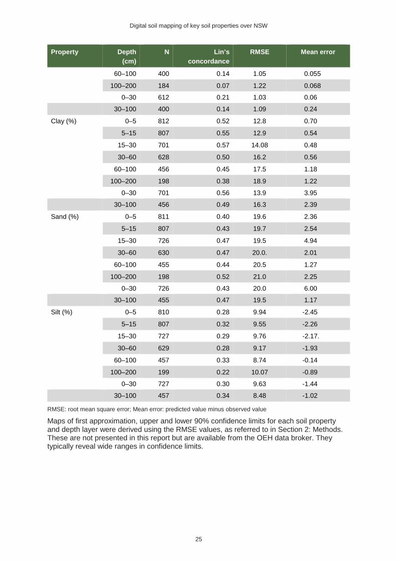
3.2 Map validation The results of map validation, using the randomly withdrawn validation datasets, are presented in Table 2. Lin’s concordance values are variable between the different soil properties and depth intervals, ranging between moderately high and low. The pH, CEC and sum-of-bases give the strongest results, with the concordance values generally ranging between 0.5 and 0.8. Low concordance values are evident for the lower depth intervals of SOC (≤0.23 below 30cm), ESP (≤0.22) and silt % (≤0.34). The concordance values have varying patterns of strength with depth for different soil properties. They increase for pH, CEC, sum-of-bases and EC; decline for SOC, ESP and clay, but remain broadly constant for P (total), sand and silt. Root mean square error values tend to increase or remain broadly constant with depth.

Table 2 Digital soil map validation results

Property Depth (cm)

N Lin’s concordance

RMSE Mean error

SOC concentration (log %)

0–5 333 0.65 0.50 -0.060

5–15 332 0.58 0.48 -0.044

15–30 331 0.43 0.57 -0.024

30–60 508 0.23 0.78 0.033

60–100 310 0.14 0.79 0.048

100–200 120 0.02 0.76 0.14

0–30 331 0.47 0.54 0.17

30–100 310 0.15 0.87 0.10

SOC mass (log kg/m3)

0–5 330 0.69 0.40 -0.0050

5–15 329 0.58 0.40 -0.0038

15–30 327 0.32 0.53 0.023

30–60 508 0.18 0.78 0.048

60–100 310 0.11 0.78 0.056

100–200 120 0.03 0.74 0.14

0–30 327 0.51 0.41 0.031

30–100 304 0.16 0.72 0.042

SOC stocks (log t/ha)

0–30 327 0.51 0.41 0.031

30–100 304 0.16 0.72 0.042

pH (pH units) 0–5 1078 0.59 0.78 -0.047

5–15 1070 0.64 0.75 -0.056

15–30 776 0.73 0.79 0.015

30–60 690 0.76 0.85 0.011

60–100 513 0.79 0.89 -0.034

100–200 239 0.77 0.98 -0.19

0–30 776 0.70 0.75 0.03


24

Property Depth (cm)


RMSE Mean error

30–100 513 0.78 0.87 0.06

CEC (log cmolc/kg)

0–5 641 0.44 0.74 -0.015

5–15 638 0.49 0.72 -0.031

15–30 603 0.57 0.69 -0.048

30–60 541 0.59 0.73 -0.062

60–100 401 0.61 0.73 -0.073

100–200 179 0.74 0.62 -0.14

0–30 603 0.51 0.71 -0.03

30–100 401 0.57 0.74 -0.05

Sum-of-bases (log cmolc/kg)

0–5 803 0.49 0.85 -0.04

5–15 800 0.53 0.83 -0.054

15–30 613 0.63 0.83 -0.032

30–60 544 0.67 0.86 -0.039

60–100 404 0.69 0.87 -0.055

100–200 183 0.79 0.77 -0.10

0–30 613 0.55 0.83 0.04

30–100 404 0.66 0.88 -0.04

P total (log mg/kg)

0–5 45 0.57 1.03 0.22

5–15 45 0.60 1.03 0.055

15–30 45 0.63 1.01 0.091

30–60 45 0.62 1.01 0.098

60–100 43 0.63 0.99 0.10

100–200 32 0.54 0.95 0.017

0–30 45 0.60 1.02 0.05

30–100 43 0.60 1.05 0.10

EC1:5 (log dS/m) 0–5 1214 0.18 0.90 0.023

5–15 1202 0.24 0.92 0.011

15–30 903 0.37 1.06 0.0051

30–60 799 0.51 1.13 -0.043

60–100 599 0.58 1.24 -0.070

100–200 270 0.56 1.36 -0.18

0–30 903 0.29 1.02 0.18

30–100 599 0.53 1.28 0.18

ESP (log %) 0–5 648 0.22 1.03 0.0098

5–15 644 0.22 1.00 0.0050

15–30 612 0.20 0.98 0.023

30–60 549 0.17 1.00 0.0075


25

Property Depth (cm)


RMSE Mean error

60–100 400 0.14 1.05 0.055

100–200 184 0.07 1.22 0.068

0–30 612 0.21 1.03 0.06

30–100 400 0.14 1.09 0.24

Clay (%) 0–5 812 0.52 12.8 0.70

5–15 807 0.55 12.9 0.54

15–30 701 0.57 14.08 0.48

30–60 628 0.50 16.2 0.56

60–100 456 0.45 17.5 1.18

100–200 198 0.38 18.9 1.22

0–30 701 0.56 13.9 3.95

30–100 456 0.49 16.3 2.39

Sand (%) 0–5 811 0.40 19.6 2.36

5–15 807 0.43 19.7 2.54

15–30 726 0.47 19.5 4.94

30–60 630 0.47 20.0. 2.01

60–100 455 0.44 20.5 1.27

100–200 198 0.52 21.0 2.25

0–30 726 0.43 20.0 6.00

30–100 455 0.47 19.5 1.17

Silt (%) 0–5 810 0.28 9.94 -2.45

5–15 807 0.32 9.55 -2.26

15–30 727 0.29 9.76 -2.17.

30–60 629 0.28 9.17 -1.93

60–100 457 0.33 8.74 -0.14

100–200 199 0.22 10.07 -0.89

0–30 727 0.30 9.63 -1.44

30–100 457 0.34 8.48 -1.02

RMSE: root mean square error; Mean error: predicted value minus observed value

Maps of first approximation, upper and lower 90% confidence limits for each soil property and depth layer were derived using the RMSE values, as referred to in Section 2: Methods. These are not presented in this report but are available from the OEH data broker. They typically reveal wide ranges in confidence limits.


26

4. Discussion

4.1 Strategy for use The digital soil maps presented here provide useful first approximations of key soil properties at different depth intervals across New South Wales, down to 100-m spatial resolutions. The maps are best viewed with GIS software, in either continuous or categorical format, although PDF images of the maps are available (as presented in Figures 2 to 13). The precise estimate for any particular pixel can be viewed using the GIS ‘identify’ tool. The validation results as presented in Table 2 are generally indicative of moderate map reliability. The upper and lower 90% confidence level maps also provide an indication of the uncertainties associated with the maps. More sophisticated techniques, such as those applied by Malone et al. (2014) and Kidd et al. (2015), may be adopted in the future to derive more reliable and narrower confidence limits. By applying the maps in conjunction with the various covariate layers (e.g. for climate, parent material and topography, as presented in Appendix 1), an understanding of the reasons behind the spatial distribution of the soil properties can be gained. For example, rising pH levels can be seen to be associated with lower rainfall, less siliceous parent materials and lower positions in the landscape.

4.2 Limitations There are a number of limitations and sources of uncertainty associated with these digital soil maps, including:

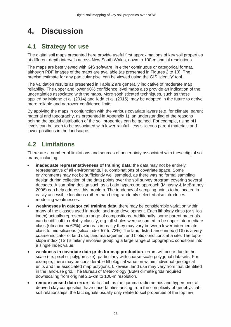
• inadequate representativeness of training data: the data may not be entirely representative of all environments, i.e. combinations of covariate space. Some environments may not be sufficiently well sampled, as there was no formal sampling design during collection of the data points over the soil survey program covering several decades. A sampling design such as a Latin hypercube approach (Minasny & McBratney 2006) can help address this problem. The tendency of sampling points to be located in easily accessible locations rather than being randomly selected also introduces modelling weaknesses.

• weaknesses in categorical training data: there may be considerable variation within many of the classes used in model and map development. Each lithology class (or silica index) actually represents a range of compositions. Additionally, some parent materials can be difficult to reliably classify, e.g. all shales were assumed to be upper-intermediate class (silica index 62%), whereas in reality they may vary between lower-intermediate class to mid-siliceous (silica index 57 to 73%).The land disturbance index (LDI) is a very coarse indicator of land use, land management and biotic conditions at a site. The topo-slope index (TSI) similarly involves grouping a large range of topographic conditions into a single index value.

• weakness in covariate data grids for map production: errors will occur due to the scale (i.e. pixel or polygon size), particularly with coarse-scale polygonal datasets. For example, there may be considerable lithological variation within individual geological units and the associated map polygons. Likewise, land use may vary from that identified in the land-use grid. The Bureau of Meteorology (BoM) climate grids required downscaling from original 2.5-km to 100-m resolution.

• remote sensed data errors: data such as the gamma radiometrics and hyperspectral derived clay composition have uncertainties arising from the complexity of geophysical–soil relationships, the fact signals usually only relate to soil properties of the top few


27

millimetres, and high noise-to-signal ratios (due to issues such as coarse resolutions and interference by water and vegetation) (McBratney et al. 2003; Mulder et al. 2011).

• time issues: the LDI does not consider the period of time a new land-use regime has been in operation, thus soil property imprints from a previous land use may still be evident in the analysed soil. The current recorded land use and groundcover may differ from that at the time of profile collection. An issue arises when soils are old enough to have been influenced by previous climatic conditions and they therefore carry an imprint from those conditions, rather than being entirely influenced by current climate conditions.

• laboratory analysis errors: including sample collection and handling errors, differences due to different laboratory techniques used and, for SOC, possible under-estimation of values by the Walkley-Black method (Skjemstad et al. 2000).

Inherent weaknesses and uncertainties in DSM are discussed more broadly in Nelson et al. (2011); Bishop et al. (2015) and Robinson et al. (2015). Despite these weaknesses, the validation results are promising and suggest the models and resulting maps are useful in providing first approximations of a range of soil properties across the landscape in New South Wales.

4.3 Relation to existing DSM and conventional soil survey products

The DSMs for New South Wales presented here represent an alternative and complementary product to the Australia-wide maps presented within the SLGA (Grundy et al. 2015; Viscarra Rossel et al. 2015). Both products are at similar scale and have the same depth intervals. However, the SLGA was prepared using modelling from data across all of Australia, while the NSW maps presented here were based on NSW data only (with exception of total P). The SLGA deals with a slightly different range of soil properties than this NSW project, with additional maps for total nitrogen, bulk density, available water-holding capacity and depth to restricting layers, but it does not include sum-of-bases (macro-nutrients), EC and ESP which are presented here. It has been contended by the SLGA Working Group that the bringing together of several DSM products derived through different methods and data sources can lead to an ultimately more reliable product (pers. comm, SLGA Working Group meeting, Canberra, 28 October 2014). This is exemplified by the combination of national and state-specific products in the primary product presented in the SLGA. These NSW maps appear to compare well with the national SLGA maps, certainly in their broad trends of spatial distribution of soil properties, however, validation statistics are generally somewhat weaker than for the SLGA maps. These new maps provide a further line of evidence for digital soil mapping results for the various soil properties. The maps also complement the conventional polygon-based eSPADE soil landscape maps available over NSW. Both products have their advantages and disadvantages. On the one hand, the DSMs provide detail of variation in soil properties within polygons. They also cover a range of soil properties that are not consistently available across the whole State. The DSMs are particularly useful where no detailed conventional soil mapping has been completed. The raster products can be more easily incorporated into many other environmental modelling programs. On the other hand, the soil landscape maps provide a more holistic overview of soil character than the individual soil properties of DSMs. They provide vital details on key soil character that are not covered by these DSMs or by DSM projects more generally. For example, they provide detail on soil type (Australian Soil Classification [ASC], Great Soil Group [GSG] or other system), profile type (uniform, gradational or texture contrast soil forms), profile depths, colour, soil structure, coarse fragments and various other macro- and micro-morphological

http://www.csiro.au/soil-and-landscape-grid



28

features. Importantly, they combine the different soil properties together into a single holistic soil description, which can be more useful and powerful than dealing with separate individual soil properties. The polygonal format of the conventional maps typically lend themselves better to applying land-use and management recommendations on the ground. Many land managers and regional planners find it useful to have discrete polygons with similar land management requirements identified for them on a map or other spatial layer, rather than a purely raster-based product.

4.4 Conclusion Digital soil maps have been produced for a range of key soil properties over New South Wales, with coverage over six soil depth intervals down to two metres. Validation results indicate at least moderate effectiveness of the maps. They are useful in providing at least a first approximation of these properties. The maps may be viewed directly through the OEH spatial viewer eSPADE and are also available for download as GIS or PDF files through the NSW Government environmental data portal SEED. Further development of the DSM techniques applied in this project, including use of other emerging remote-sensed datasets, and application of more sophisticated measures of map uncertainty, will improve the quality and effectiveness of these maps. The DSMs are a potentially useful complementary product to the existing digital soil maps and conventional soil landscape products available for much of New South Wales. Both the digital and conventional soil products can be used together to help inform on soil conditions throughout the State. They can thus assist in the ongoing sustainable management and protection of this vital natural resource. These also provide valuable input data for a range of other natural resource and environmental modelling systems, critical for effective environmental management across the State.


https://datasets.seed.nsw.gov.au/dataset/digital-soil-maps-for-key-soil-properties-over-nsw


29

Appendix 1: Covariate layers

Figure A1.1 Annual rainfall (mm pa)

Figure A1.2 Mean annual daily max temperature (oC)

Figure A1.3 Lithology and silica content (%)

Figure A1.4 Radiometric K (%)


30

Figure A1.5 Radiometric U (mg/kg)

Figure A1.6 Radiometric Th (mg/kg)

Figure A1.7 Kaolin (component fraction)

Figure A1.8 Illite (component fraction)


31

Figure A1.9 Smectite (component fraction)

Figure A1.10 Smectite/kaolin ratio

Figure A1.11 Topographic wetness index

(TWI)

Figure A1.12 Topo-slope index (TSI)


32

Figure A1.13 Slope (%)

Figure A1.14 Aspect index

Figure A1.15 Land disturbance index (LDI)

Figure A1.16 Ground cover (%)


33

Figure A1.17 Weathering index


34

Appendix 2: Multiple linear regression models (derived from training datasets)

Soil property

Depth (cm)

Multiple linear regression equation N R2 RSE1

SOC concentration (%)

0-5 = exp(3.007+0.000758*rain-0.0659*tmax-0.0254*silica-0.180*rad_k+1.509*kaolin-2.146*illite-0.0850*ldi +0.00688*ground_cov -0.0444*w_i)

1204 0.55 0.43

5-15 = exp(2.623+0.000783*rain-0.0513*tmax-0.0265*silica-0.119*rad_k-0.124*rad_u+1.373*kaolin-2.221*illite +0.0135*tsi-0.0656*ldi+0.00396*ground_cov -0.0260*w_i)

1203 0.52 0.39

15-30 = exp(3.439+0.000870*rain-0.0343*tmax-0.0297*silica-0.125*rad_k-0.112*rad_u-0.0244*rad_th +0.748*kaolin-3.509*illite+0.0141*tsi-0.0655*ldi-0.00599*ground_cov)

1200 0.40 0.47

30-60 = exp(0.8057+0.000571*rain-0.0422*tmax-0.0205*silica-1.358*illite+4.516*smectite-1.155*sk_ratio2+0.0601*tsi-0.0289*twi+0.00658*slope-0.0238*ldi+0.0604*w_i)

1935 0.21 0.74

60-100 =exp(0.564+0.000362*rain-0.0339*tmax-0.0170*silica-0.0146*rad_th+0.0606*tsi-0.0327*twi+0.00707*slope +0.0328*w_i)

1249 0.14 0.72

100-200 = exp(-1.087+0.000293*rain-0.0119*silica+0.0369*tsi+0.00449*ground_cov) 471 0.06 0.78

SOC mass (kg/m3)

0-5 = exp(4.644+0.000449*rain-0.0501*tmax-0.0177*silica-0.155*rad_k+1.834*kaolin-1.195*illite-0.0189*twi-0.0667*ldi+0.00652*ground_cov -0.0364*w_i)

1203 0.53 0.39

5-15 = exp(4.850+0.000541*rain-0.0420*tmax-0.0206*silica-0.115*rad_k-0.0558*rad_u-0.00817*rad_th +1.654*kaolin-1.750*illite-0.0107*twi-0.0540*ldi+0.00239*ground_cov -0.0276*w_i)

1201 0.47 0.37

15-30 = exp(5.901+0.000667*rain-0.0279*tmax-0.0237*silica-0.156*rad_k-0.0719*rad_u-0.0249*rad_th +0.908*kaolin-3.041*illite+0.0188*tsi-0.0180*twi-0.0623*ldi-0.00700*ground_cov -0.0324*w_i)

1198 0.33 0.45

30-60 = exp(3.175+0.000498*rain-0.0448*tmax-0.0185*silica+4.149*smectite-1.102*sk_ratio2+0.0584*tsi-0.0320*twi+0.00615*slope+0.0569*w_i)

1980 0.17 0.73

60-100 = exp(2.353+0.000188*rain-0.0245*tmax-0.0166*silica-0.0118*rad_th+1.346*kaolin+0.0690*tsi-0.0287*twi+0.00762*slope+0.0295*w_i)

1271 0.12 0.70

100-200 = exp(1.215+0.000122*rain-0.0116*silica+0.742*kaolin+0.0554*tsi+0.0542*asp+0.00396*ground_cov) 488 0.06 0.76

0-30 2 =exp(4.832+0.000586*rain-0.0395*tmax-0.0203*silica5-0.123*rad_k-0.0164*rad_th+1.495*kaolin-1.820*illite+0.00948*tsi-0.0601*ldi4-0.0302*w_i)

1181 0.43 0.37

30-100 2 = exp(2.916+0.000278*rain-0.0263*tmax-0.0207*silica+1.478*kaolin-1.797*illite+0.0679*tsi-0.0370*twi +0.00660*slope+0.00170*ground_cov+0.0506*w_i)

1257 0.18 0.69


35

Soil property

Depth (cm)


pH (CaCl2) 0-5 = 5.416-0.000527*rain+0.0607*tmax-0.0183*silica+0.248*rad_k-0.0611*rad_u-0.0299*rad_th-1.837*kaolin-1.136*illite+3.450*smectite+0.0343*twi+0.00750*slope+0.0645*ldi-0.00115*ground_cov+0.0294*w_i

3911 0.47 0.70

5-15 = 5.641-0.000553*rain+0.0594*tmax-0.0187*silica+0.249*rad_k-0.0576*rad_u-0.0304*rad_th-2.281*kaolin-1.063*illite+3.780*smectite+0.0362*twi+0.00765*slope+0.0598*ldi-0.00110*ground_cov+0.0322*w_i

3879 0.52 0.68

15-30 = 6.925-0.000661*rain+0.0594*tmax-0.0212*silica+0.156*rad_k-0.148*rad_u-4.903*kaolin+1.127*Illite +5.107*smectite -1.077*sk_ratio2+0.0789*tsi+0.0286*twi+0.00881*slope+0.0181*asp+0.0982*ldi-0.00135*ground_cov

2827 0.61 0.73

30-60 = 8.052-0.000898*rain+0.0659*tmax-0.0222*silica+0.153*rad_k-0.172*rad_u-6.741*kaolin+1.187*illite +6.548*smectite-1.938*sk_ratio2+0.0840*tsi+0.0422*twi+0.00953*slope+0.0190*asp+0.114*ldi-0.00136*ground_cov

2526 0.62 0.80

60-100 = 10.20-0.00117*rain+0.0798*tmax-0.0221*silica+0.172*rad_k-0.225*rad_u-9.072*kaolin+6.909*smectite-2.882*sk_ratio2+0.0796*tsi+0.0321*twi+0.00736*slope+0.123*ldi-0.00171*ground_cov

1823 0.64 0.89

100-200 = 10.626-0.00134*rain+0.0925*tmax-0.0212*silica+0.246*rad_k-0.147*rad_u-0.0282*rad_th-9.106*kaolin +6.927*smectite-3.212*sk_ratio2+0.0544*twi+0.141*ldi-0.00396*ground_cov

811 0.65 0.95

CEC (cmolc/kg)

0-5 = exp(4.376-0.000157*rain+0.0197*tmax-0.0426*silica-0.138*rad_u+1.921*smectite+0.0582*tsi-0.0229*twi +0.00562*slope+0.0234*asp+0.0579*ldi)

2535 0.41 0.68

5-15 = exp(4.074-0.000196*rain+0.0265*tmax-0.0439*silica-0.109*rad_k+2.45*smectite+0.0570*tsi-0.0212*twi +0.00627*slope+0.0229*asp+0.0727*ldi)

2493 0.44 0.66

15-30 = exp(4.256-0.000251*rain+0.0325*tmax-0.0459*silica-0.0563*rad_u-0.0225*rad_th+2.39*smectite+0.0437*tsi-0.0187*twi+0.00513*slope+0.0185*asp+0.0849*ldi-0.00108*ground_cov+0.0336*w_i)

2309 0.50 0.69

30-60 = exp(4.113-0.000352*rain+0.0507*tmax-0.0463*silica+0.0736*rad_k-0.0734*rad_u-0.0277*rad_th+1.592*smectite +0.127*ldi+0.0223*w_i)

2091 0.49 0.71

60-100 = exp(4.288-0.000435*rain+0.0484*tmax-0.0453*silica+0.107*rad_k-0.0771*rad_u-0.0214*rad_th+1.544*smectite +0.127*ldi)

1558 0.49 0.72

100-200 = exp(3.938-0.000544*rain+0.0574*tmax-0.0459*silica-0.153*rad_u+2.499*illite+1.071*smectite+0.0922*ldi 685 0.55 0.71

Sum-of-bases (cmolc/kg)

0-5 = exp(3.103-0.000361*rain+0.0696*tmax-0.0433*silica+0.171*rad_k-0.0998*rad_u-0.0479*rad_th+2.17*smectite +0.00852*slope+0.0191*asp+0.0741*ldi+0.0254*w_i)

3171 0.43 0.78

5-15 = exp(2.957-0.000398*rain+0.0731*tmax-0.0445*silica+0.156*rad_k-0.0882*rad_u-0.0481*rad_th+2.561*smectite +0.00902*slope+0.0194*asp+0.0910*ldi+0.0263*w_i)

3130 0.46 0.76


36

Soil property

Depth (cm)


15-30 = exp(2.585-0.000560*rain+0.0766*tmax-0.0503*silica+0.154*rad_k-0.135*rad_u-0.0376*rad_th+1.916*Illite +3.782*smectite-0.579*sk_ratio2+0.0660*tsi-0.0179*twi+0.0121*slope+0.0249*asp +0.160*ldi +0.0452*w_i)

2353 0.55 0.78

30-60 = exp(3.398-0.000840*rain+0.0832*tmax-0.0521*silica+0.194*rad_k-0.157*rad_u-0.0366*rad_th+1.489*Illite +0.717*smectite+0.0406*tsi+0.0104*slope+0.202*ldi-0.00136*ground_cov+0.0383*w_i)

2114 0.56 0.83

60-100 = exp(3.425-0.00104*rain+0.0950*tmax-0.0496*silica+0.266*rad_k-0.189*rad_u-0.0303*rad_th+1.398*Illite +0.0414*tsi+0.00771*slope+0.192*ldi)

1568 0.56 0.86

100-200 = exp(4.074-0.00114*rain+0.102*tmax-0.0531*silica+0.283*rad_k-0.217*rad_u-0.0239*rad_th+0.190*ldi) 686 0.61 0.89

P total (mg/kg)

0-5 = exp(10.089+0.000811*rain-0.0430*silica-6.156*kaolin+5.948*illite+2.800*smectite-1.741*sk_ratio- 0.0543*twi+0.0669*w_i)

1335 0.34 0.84

5-15 = exp(10.46+0.000865*rain-0.0422*silica-6.884*kaolin+5.441*illite+2.783*smectite-1.840*sk_ratio-0.0577*twi+0.0761*w_i)

1317 0.34 0.84

15-30 = exp(11.76+0.000733*rain-0.0150*tmax-0.0441*silica-7.930*kaolin+6.641*illite-1.406*sk_ratio-0.0694*twi+0.0795*w_i)

1145 0.35 0.84


1064 0.36 0.84


851 0.39 0.84

100-200 = exp(10.075+0.000562*rain-0.0478*silica-4.412*kaolin+3.565*illite-0.0806*twi) 579 0.33 0.88

EC1:5 (dS/m) 0-5 = exp(-3.361+0.0000604*rain+0.0267*tmax-0.00915*silica-0.0181*rad_th+1.368*kaolin-2.169*illite-2.375*smectite+1.065*sk_ratio2+0.0838*tsi+0.0247*twi+0.0390*asp+0.0524*ldi)

4642 0.13 0.78

5-15 = exp(-2.552+0.0271*tmax-0.00990*silica-0.0199*rad_th-2.283*illite-2.081*smectite+0.852*sk_ratio2+0.0921*tsi +0.0238*twi+0.0407*asp+0.0442*ldi+0.0275*w_i)

4525 0.17 0.80

15-30 = exp(-2.447-0.000143*rain+0.0373*tmax-0.0122*silica-0.121*rad_k+0.0935*rad_u-0.0217*rad_th-3.675*illite-1.443*smectite+0.827*sk_ratio2+0.128*tsi+0.0403*twi+0.0325*asp+0.0706*ldi-0.00154*ground_cov)

3319 0.31 0.87

30-60 = exp(-2.560-0.000288*rain+0.0573*tmax-0.0146*silica-0.118*rad_k+0.0714*rad_u-0.0130*rad_th-4.107*illite-2.387*smectite+1.298*sk_ratio2+0.135*tsi+0.0592*twi+0.0790*ldi-0.00298*ground_cov)

3049 0.40 0.98

60-100 = exp(-3.038-0.000341*rain+0.0889*tmax-0.0170*silica+0.0848*rad_u-0.0169*rad_th-4.369*illite-2.836*smectite +1.531*sk_ratio2+0.136*tsi+0.0701*twi+0.0620*ldi-0.00458*ground_cov+0.0523*w_i)

2206 0.46 1.12

100-200 = exp(-4.188-0.000444*rain+0.124*tmax-0.0196*silica+0.216*rad_u-0.0254*rad_th-5.849*illite+1.498*smectite +0.145*tsi+0.123*twi+0.161*ldi-0.00334*ground_cov)

983 0.41 1.32


37

Soil property

Depth (cm)


ESP (%) 0-5 = exp(-2.726+0.000482*rain+0.0175*tmax+0.0314*silica-0.196*rad_k+0.163*rad_u+2.067*kaolin-3.748*smectite +1.416*sk_ratio2+0.0432*tsi+0.0483*twi-0.00354*slope-0.0774*ldi-0.0824*w_i)

2496 0.16 1.10

5-15 = exp(-2.919+0.000424*rain+0.0229*tmax+0.0321*silica-0.155*rad_k+0.137*rad_u+2.481*kaolin-4.222*smectite +1.691*sk_ratio2+0.0394*tsi+0.0517*twi-0.00491*slope-0.0862*ldi-0.0832*w_i)

2476 0.17 1.05

15-30 = exp(-0.992+0.000336*rain+0.0283*tmax+0.0306*silica-0.166*rad_k+0.151*rad_u-3.27*smectite+0.779*sk_ratio2 +0.0329*tsi+0.0425*twi-0.00664*slope-0.0942*ldi-0.0838*w_i)

2320 0.17 1.00

30-60 = exp(-1.423+0.000293*rain+0.0378*tmax+0.0277*silica-0.125*rad_k+0.156*rad_u+0.0555*tsi+0.0477*twi-0.00428*slope-0.112*ldi-0.0759*w_i)

2133 0.15 1.02

60-100 = exp(0.161+0.000227*rain+0.0359*tmax+0.0230*silica-0.159*rad_k+0.130*rad_u-1.878*illite-6.680*smectite +2.012*sk_ratio2+0.0860*tsi+0.0344*twi-0.0506*ldi-0.00247*ground_cov-0.0741*w_i)

1543 0.12 1.07

100-200 = exp(-0.850+0.0624*tmax+0.0225*silica-0.00409*ground_cov) 707 0.06 1.15

Clay (%) Cubist models (not presented)

Sand (%) Cubist models (not presented)

Silt (%) Cubist models (not presented)

1 RSE: residual standard error (in natural log scale for SOC, CEC, sum-of-bases, P total, EC, and ESP 2 SOC mass converted to SOC stocks (Mg/ha) using conversion factors


38

References Arrouays D, McKenzie N, Hempel J, Richer de Forges A, McBratney A (Eds) 2014, GlobalSoilMap: Basis of the global spatial soil information system, CRC Press/Balkema, The Netherlands. Baldock JA, Wheeler I, McKenzie N, McBratney A 2012, Soils and climate change: potential impacts on carbon stocks and greenhouse gas emissions, and future research for Australian agriculture, Crop and Pasture Science 63, 269–283. Brus DJ, Kempen B, Heuvelink GBM 2011, Sampling for validation of digital soil maps, European Journal of Soil Science 62, 394–407. Bishop TFA, Horta A, Karunaratne SB 2015, Validation of digital soil maps at different spatial supports, Geoderma 241–242, 238–249. Bishop TFA, McBratney AB, Laslett GM 1999, Modelling soil attribute depth functions with equal-area quadratic smoothing splines, Geoderma 91, 27–45. Bui E, Henderson B, Viergever K 2009, Using knowledge discovery with data mining from the Australian Soil Resource Information System database to inform soil carbon mapping in Australia, Global Biogeochemical Cycles 23, 1–15. Chapman GA, Gray JM, Murphy BW, Atkinson G, Leys JF, Muller R, Peasely B, Wilson BR, Bowman, G, McInnes-Clarke SK, Tulau MJ, Morand, DT, Yang X 2011, Monitoring, Evaluation and Reporting of Soil Condition in New South Wales: 2008 Program. NSW Department of Environment, Climate Change and Water, Sydney, www.environment.nsw.gov.au/resources/soc/20110718SoilsTRS.pdf (accessed 6.5.2017). Dokuchaev VV 1899, On the Theory of Natural Zones, St. Petersburg, Russia. Gallant JC, Austin JM 2015, Derivation of terrain covariates for digital soil mapping in Australia, Soil Research 53, 895–90. Guerschman JP, Hill MJ, Renzullo LJ, Barrett DJ, Marks AS, Botha EJ 2009, Estimating fractional cover of photosynthetic vegetation, non-photosynthetic vegetation and bare soil in the Australian tropical savanna region upscaling the EO-1 Hyperion and MODIS sensors, Remote Sensing of Environment 113, 928–45. Gray JM, Bishop TFA, Wilford JR 2016, Lithology and soil relationships for soil modelling and mapping, Catena 147, 429–440, doi.org/10.1016/j.catena.2016.07.045. Gray JM, Bishop TFA, Wilson BR 2015a, Factors controlling soil organic carbon stocks with depth in eastern Australia, Soil Science Society of America Journal 79, 1741–1751, doi:10.2136/sssaj2015.06.0224. Gray JM, Bishop TFA, Yang X 2015b, Pragmatic models for the prediction and digital mapping of soil properties in eastern Australia, Soil Research 53, 24–42, doi:10.1071/SR13306. Grundy MJ, Viscarra Rossel RA, Searle RD, Wilson PL, Chen C, Gregory LJ 2015, Soil and Landscape Grid of Australia, Soil Research 53, 835–844. Henderson BL, Bui EN 2002, An improved calibration curve between soil pH assessed in water and CaCl2, Australian Journal of Soil Research 40, 1399–1405. Henderson BL, Bui EN, Moran CJ, Simon DAP 2005, Australia-wide predictions of soil properties using decision trees, Geoderma 124, 383–398. Isbell RF 2002, Revised Edition of the Australian Soil Classification, CSIRO Australia, Melbourne.

http://www.environment.nsw.gov.au/resources/soc/20110718SoilsTRS.pdf


39

Jenny H 1941, Factors of soil formation, McGraw-Hill Book Company, New York. Kidd D, Webb M, Malone B, Minasny B, McBratney AB 2015, Digital soil assessment of agricultural suitability, versatility and capital in Tasmania, Australia, Geoderma Regional 6, 7–21. Kuhn M, Weston S, Keefer C, Coulter N, Quinlan R 2014, Cubist: Rule- and Instance-Based Regression Modeling, R package version 0.0.18, http://CRANR-project.org/package=Cubist (accessed 22.3.2016). Karunaratne SB, Bishop TFA, Baldock JA, Odeh IOA 2014, Catchment scale mapping of measureable soil organic carbon fractions, Geoderma 219–220, 14–23. Lin LI 1989, A concordance correlation coefficient to evaluate reproducibility, Biometrics 45, 255–268. Malone BP, McBratney AB, Minasny B, Laslett GM 2009, Mapping continuous depth functions of soil carbon storage and available water capacity, Geoderma 154, 137–52. Malone BP, Minasny B, Odgers NP, McBratney AB 2014, Using model averaging to combine soil property rasters from legacy soil maps and from point data, Geoderma 232–234, 34–44. McBratney AB, Mendonça Santo ML, Minasny B 2003, On digital soil mapping, Geoderma 117, 3–52. Minasny B, McBratney AB 2006, A conditioned Latin hypercube method for sampling in the presence of ancillary information, Computer Geoscience 32, 1378–1388. Minasny B, McBratney AB, Mendonça-Santos ML, Odeh IOA, Guyon B 2006, Prediction and digital mapping of soil carbon storage in the Lower Namoi Valley, Australian Journal of Soil Research 44, 233–244. Mulder VL, De Bruin S, Schaepman ME, Mayr TR 2011, The use of remote sensing in soil and terrain mapping — a review, Geoderma 162, 1–19. Nelson MA, Bishop TFA, Odeh IOA, Triantafilis J 2011, An error budget for different sources of error in digital soil mapping, European Journal of Soil Science 62, 417–430. Odeh, IOA, McBratney AB, Chittleborough DI 1995, Further results on prediction of soil properties from terrain attributes: heterotopic cokriging and regression-kriging, Geoderma 67, 215–226. OEH 2007, Land use mapping for NSW, NSW Office of Environment and Heritage. OEH 2014, Soil condition and land management in NSW: Final results from the 2008–09 monitoring evaluation and reporting program, Technical Report, NSW Office of Environment and Heritage, Sydney, www.environment.nsw.gov.au/soils/140389MERsoil.htm (accessed 6.5.2017). NSW Department of Resources and Energy, undated, 1:250 000 Geological Maps. www.resourcesandenergy.nsw.gov.au/miners-and-explorers/geoscience-information/products-and-data/maps/geological-maps (accessed 6.5.2017). Rayment GE, Lyons DJ 2011, Soil Chemical Methods – Australasia, Australian Soil and Land Survey Handbook Series, CSIRO Publishing, Melbourne. Quinlan J 1992, Learning with continuous classes, in: Adams A, Sterling L (Eds), AI’92: Proceedings of the 5th Australian Joint Conference on Artificial Intelligence, World Scientific, Singapore, pp. 343–348. Reuter HI 2011, JMP and CUBIST Prediction Toolbox, www.globalsoilmap.net/content/globalsoilmapnet-prediction-toolbox (accessed 29.9.2016).

http://cran.r-project.org/package=Cubist

http://www.environment.nsw.gov.au/soils/140389MERsoil.htm

http://www.resourcesandenergy.nsw.gov.au/miners-and-explorers/geoscience-information/products-and-data/maps/geological-maps

http://www.resourcesandenergy.nsw.gov.au/miners-and-explorers/geoscience-information/products-and-data/maps/geological-maps

http://www.globalsoilmap.net/content/globalsoilmapnet-prediction-toolbox


40

Robinson NJ, Benke KK, Norng S 2015, Identification and interpretation of sources of uncertainty in soils change in a global systems-based modelling process, Soil Research 53, 592–604. R Core Team 2013, R: A language and environment for statistical computing, R Foundation for Statistical Computing, Vienna, Austria, www.R-project.org/ (accessed: 22.3.2016). Sanchez PA, Ahamed S, Carré F, Hartemink A, Hempel J, Huising J, Lagacherie P, McBratney A, McKenzie N, de Lourdes Mendonça-Santos M, Minasny B, Montanarella L, Okoth P, Palm C, Sachs J, Shepherd K, Vågen T, Vanlauwe B, Walsh M, Winowiecki L, Zhang G 2009, Digital soil map of the world, Science 325, 680–681. Sanderman J, Baldock J, Hawke B, Macdonald L, Massis-Puccini A, Szarvas S 2011, National Soil Carbon Research Programme: Field and Laboratory Methodologies, CSIRO Land and Water, Urrbrae, South Australia, https://csiropedia.csiro.au/wp-content/uploads/2016/06/SAF-SCaRP-methods.pdf (accessed 17.10.2016). Skjemstad JO, Spouncer LR, Beech A 2000, Carbon conversion factors for historical soil carbon data, Technical Report No. 15, National Carbon Accounting System, Australian Greenhouse Office, Canberra. Triantafilis J, Lesch SM, Lau KL, Buchanan SM 2009, Field level digital soil mapping of cation exchange capacity using electromagnetic induction and a hierarchical spatial regression model, Australian Journal of Soil Research 47, 651–663.

Viscarra Rossel RA 2011, Fine‐resolution multiscale mapping of clay minerals in Australian soils measured with near infrared spectra, Journal of Geophysical Research 116, F04023, 15p. Viscarra Rossel RA, Chen C, Grundy M, Searle R, Clifford D, Campbell PH 2015, The Australian three-dimensional soil grid: Australia's contribution to the GlobalSoilMap project, Soil Research 53, 845–864. Viscarra Rossel RA, Webster R, Bui EN, Baldock JA 2014, Baseline map of organic carbon in Australian soil to support national carbon accounting and monitoring under climate change, Global Change Biology 20, 2953–2970. Wilford J 2012, A weathering intensity index for the Australian continent using airborne gamma-ray spectrometry and digital terrain analysis, Geoderma 183, 124–142.

http://www.r-project.org/

https://csiropedia.csiro.au/wp-content/uploads/2016/06/SAF-SCaRP-methods.pdf

https://csiropedia.csiro.au/wp-content/uploads/2016/06/SAF-SCaRP-methods.pdf

digital soil mapping of key soil properties over new …...digital soil mapping of key soil...

Documents