digital signal processing for coherent communication and...
TRANSCRIPT

i
Digital Signal Processing for Coherent Communication and
Compensation of Photonic Integration Imperfections
Tadesse S.Mulugeta
Promotor: prof. dr. Geert Morthier
Supervisor: Dr. Christopher R. Doerr
Master dissertation submitted in order to obtain the academic degree of
Erasmus Mundus Master of Science in Photonics
Academic year 2011-2012

ii

iii
Digital Signal Processing for Coherent Communication and
Compensation of Photonic Integration Imperfections
Tadesse S.Mulugeta
Promotoren: prof. dr. Geert Morthier
Begeleider: Dr. Christopher R. Doerr
Masterproef ingediend tot het behalen van de academische graad van
Erasmus Mundus Master of Science in Photonics

iv
Acknowledgements
I am very fortunate to have Dr. Christopher R. Doerr as my supervisor. Since the time I asked to
do my thesis under his supervision in Acacia Communication, his willingness to help me, his
immense knowledge, patience and the way he bring light to any of my difficulties have been
amazing. I am greatly indebted to him, I simply say: thank you so much.
I would also like to greatly thank my promoter Prof. Geert Morthier, for his concern and giving
me his feedbacks on the thesis work.
I owe a great deal of thanks to Prof. Roel Baets for giving me the permission to do my master
thesis in Acacia Communication.
My sincere gratitude goes to the European Commission for sponsoring me through the Erasmus
Mundus program. It would have been unthinkable to persuade my master study abroad without
the scholarship.
Special thanks to Diedrik Vermeulen, who not only has given me a ride in his car, but has been
instrumental in my work with his feedback and courage.
My many thanks are also to the staff member of Acacia communication who helped me a lot
(especially to Jonas Geyer, Graeme Pendock, Long Chen, Scott Stulz, Mehmet Aydinlik, Saeid
Azemati and Seo Yeon Park).
Nebiyu Adello, thank you for encouraging me during my studies and giving me your feedback in
my write up.
Finally, my deepest gratitude goes to my family for their never ending support, guidance, love
and care.

v
Permission for usage (English version)
The work in this thesis is not yet approved by Acacia Communications for public release.
Acacia needs to review the thesis and possibly remove some content before a public release.
Tadesse Mulugeta
17 June 2012

vi
Abstract
Coherent detection in combination with digital signal processing (DSP) provides new
capabilities such as enabling the use of highly spectrally efficient modulation formats and
compensating a wide variety of transmission impairments. However, coherent transceivers are
extremely complex and contain many interconnected optical and electrical components. Photonic
integrated circuits (PICs) are a key technology to not only reduce the complexity, cost, and
footprint of the transceivers but enable future scaling. PICs do have design trade-offs due to the
integration, and these need a deeper understanding.
In this thesis, the most important DSP algorithms used for coherent receiver are studied and
simulations are performed. Many PIC imperfections are discussed, and novel DSP mitigation
techniques for compensation of some of the imperfections are proposed, simulated, and, in one
case, experimentally demonstrated.

vii
List of Figures
Figure.2.1.Constellation diagrams of most common optical modulation formats. ......................... 5
Figure.2.2 Three categories of Coherent detection. (a) homodyne, (b) intradyne, and (c)
heterodyne. ...................................................................................................................................... 6
Figure.2.3 Coherent receiver types.(a) single quadrature, (b) dual quadrature, and (c) dual
polarization, dual quadrature. [10] .................................................................................................. 7
Figure 2.4: Optical coherent communication link.[10] ................................................................... 8
Figure.2.5. Layout of Si dual polarization, dual-quadrature coherent receiver [11] ...................... 9
Figure.6 QPSK constellation diagram for different types of imperfection. Borrowed from [15] 10
Figure.3.1. Coherent receiver employing phase and polarization diversity. [1] ........................... 14
Figure.3.2. 900 Optical Hybrid [1] ............................................................................................... 15
Figure.3.3. DSP block diagrams for dual polarization phase diversity receiver [1]. .................... 15
Figure.3.4. Phase response of dispersive fiber for several fiber length[4]. .................................. 17
Figure.3.5 Schematic of an FIR filter for compensating chromatic dispersion ............................ 17
Figure.3.6. Polarization de-multiplexing equalization filters architecture. .................................. 19
Figure.3.7 Feed-forward phase estimation algorithm for QPSK modulation. .............................. 22
Figure.3.8. PDM-QPSK Digital signal processing ....................................................................... 23
Figure.3.9. PDM-16QAM Digital signal processing .................................................................... 24
Figure.4.1. Dual Parallel MZM with unequal splitting ratio ........................................................ 27
Figure.4.2. Constellation diagrams of 16QAM using non-ideal MZM ........................................ 30
Figure.4.3 Transmitter block-diagram .......................................................................................... 31
Figure.4.4 Transmitter block-diagram involving linear filters and non-linear equalizers. [Partly
from 14] ........................................................................................................................................ 32
Figure 4.5 Phase diagrams and constellation diagrams without and with compensation of
bandwidth limitation in the transmitter for a 120-Gb/s PDM-QPSK signal. ................................ 33
Figure.4.6 various type of Si modulator (a) carrier injection (b) carrier depletion (c) MOS [15] 34
Figure.4.7. Relative phase shift and normalized capacitance at different phase shifter voltages.
[6] .................................................................................................................................................. 35
Figure.4.8. (a) Dual-Parallel MZM, (b) approximate linear filter equivalence for single MZM . 37
Figure.4.9 (a) capacitance curve piecewise approximation (b) equalizing filters amplitude
response......................................................................................................................................... 38
Figure.4.10 constellation and eye diagram for 16QAM Si-modulator ......................................... 39
Figure.4.11. Constellations diagram (a) with QI and frequency offset of 10MHz. (b) QI
compensated. (c) QI and frequency offset compensated. ............................................................ 42
Figure.4.12.16-QAM constellation points and QPSK partitioning............................................... 43
Figure 4.13.Constellation diagrams for 16-QAM signal with 15 degree hybrid phase error and
unequal photodiodes responsivity ................................................................................................. 43
Figure.4.14 Constellation diagram illustrating the effect of 90 degree phase error at MZM and
hybrid detector .............................................................................................................................. 46
Figure.5.1. Offline processing test set up ..................................................................................... 49

viii
Figure.5.2 Constellation diagrams illustrating sequence of DSP processing on the real PDM-
QPSK signal. 120.5784Gb/s, 20dB OSNR ................................................................................... 50
Figure.5.3 BER performance at 30.1446 Gbaud: dual-polarization 120.5784Gb/s QPSK .......... 51
Figure.5.4. BER versus LO power for 0dBm signal power. The green square after nonlinear
equalization is for 15.5 dBm LO power........................................................................................ 51

ix
LIST OF ACRONYMS
ADC Analog to digital convertor
ASE Amplified spontaneous emission
ASIC Application specific integration circuit
BPSK Binary phase shift keying
CD Chromatic dispersion
CMOS Complementary Metal Oxide Semiconductor
DAC Digital to analog convertor
DB Duobinary
DC Direct current
DSP Digital signal processing
EDFA Er-doped fiber amplifier
EIC Electronic integrated circuit
FEC Forward-error correction
GSOP Gram-Schmidt Orthogonalization procedure
GVD Group velocity dispersion
ITLA Integrable tunable laser assembly
LO Local oscillator
OOK On-off keying
PDL Polarization dependent loss
PDM Polarization division multiplexing
PIC Photonic integrated circuit
PMD Polarization mode dispersion
Pol-SK Polarization shift keying
PRBS Pseudo-random binary sequences

x
QAM Quadrature amplitude modulation
QPSK Quadrature phase shift keying
RF Radio frequency
SE Spectral efficiency
TIA Transimpedance amplifier
WDM Wavelength division multiplexing

xi
Contents 1. Introduction .............................................................................................................................................. 1
1.1 Introduction ........................................................................................................................................ 1
1.2 Motivation .......................................................................................................................................... 2
1.3 Report outline .................................................................................................................................... 2
1.4 References .......................................................................................................................................... 3
2. Background ............................................................................................................................................... 4
2.1 Advanced modulation Formats ......................................................................................................... 4
2.2 Coherent Receiver .............................................................................................................................. 5
2.3 Photonic Integrated Circuit ................................................................................................................ 7
2.4 Photonic integrated circuit imperfection. ......................................................................................... 9
2.5 References ........................................................................................................................................ 11
3. Digital Signal Processing For Coherent Optical Communications ......................................................... 12
3.1 Introduction ...................................................................................................................................... 12
3.3 Chromatic Dispersion Compensation .............................................................................................. 16
3.4 Polarization de-multiplexing ............................................................................................................ 18
3.5 Frequency offset estimation ............................................................................................................ 21
3.6 Carrier phase estimation .................................................................................................................. 22
3.8 Simulation result .............................................................................................................................. 23
3.8 References ........................................................................................................................................ 25
4. Compensation of Photonic Integrated Circuit Imperfection ................................................................ 26
4.1 Introduction ...................................................................................................................................... 26
4.2 Compensation limited extinction ratio at MZM ............................................................................. 26
4.3 Compensation of limited bandwidth and non-linearity ................................................................. 30
4.4 Compensation of varying capacitance in silicon-modulator .......................................................... 33
4.5 Compensation of imperfect hybrid phase and photodiodes responsivity mismatch .................... 39
4.6 Compensation of 90 degree phase error at MZM ........................................................................... 44
4.7 References ........................................................................................................................................ 47

xii
5. Experimental result and analysis ........................................................................................................... 48
5.1 Introduction ...................................................................................................................................... 48
5.2 Experimental set up ......................................................................................................................... 48
5.3 Result and analysis ........................................................................................................................... 49
6. Conclusion and recommendations ........................................................................................................ 53
6.1 conclusions ....................................................................................................................................... 53
6.2 Future work ...................................................................................................................................... 54

1
CHAPTER 1
1. INTRODUCTION
1.1 Introduction
Fiber optic communication is a method of conveying information from one place to another by
sending pulses of light through an optical fiber. The light forms an electromagnetic carrier wave
that is modulated with the information signal. Due to the high carrier frequency of roughly of
200THz, 200,000 times a typical microwave carrier frequency, much higher data transmission
rate can be achieved in fiber-optic system. [1] Within the last 30 years, the transmission capacity
of optical fibers, which have a low-loss bandwidth of ~10 THz, has been increased enormously.
Fiber optic communication has revolutionized the telecommunication industry and has played a
major role in the field of data communication.
Compared to traditional copper wire, optical fiber has many advantages such as: its much lower
attenuation, high immunity from electrical interference, light weight and huge data transmission
capacity. As a result, it has been a choice for many telecommunication companies especially for
long distance and high demand applications. Driven by the exponential growth of data traffic,
high-capacity optical transmission has experienced orders of magnitude growth in capacity in the
past two decades. The capacity growth has been enabled by key technology breakthroughs such
as the erbium-doped fiber amplifier (EDFA), wavelength-division multiplexing (WDM),
dispersion compensation and management, and fiber nonlinearity management [4].
Today network traffic continues to grow exponentially driven by bandwidth hungry digital
applications, video-on-demand, telepresence, wireless backhaul, cloud computing & services,
etc. To keep up with this unprecedented traffic growth, the transmission capacity of fiber optics
has to be increased further. However, high bit rate optical transmission is limited by optical
impairments such as chromatic dispersion, attenuation, and nonlinearity. These impairments
limit the available bandwidth in the fiber as well as the transmission reach. For years these
impairments have been dealt with in the optical domain through optical components such as
erbium-doped fiber amplifiers (EDFA) to compensate the attenuation introduced by the fiber or
dispersion compensating fibers (DCF) to undo chromatic dispersion of the fiber. These methods
however do have several drawbacks such as their high cost, large physical size, additional loss,
latency, and lack of flexibility.
Recent developments in high speed electronic DSP technology created a new paradigm in optical
communication. The realization of high throughput DSP devices has enabled compensation of
fiber optic impairment electronically. Thus, one can have more adaptability, reduced cost and
simplification in the optical link.
In conjunction with coherent detection, where the field rather than the power is detected, DSP
enables the adoption of more spectrally efficient modulation formats and extends the electronic

2
mitigation possibility. Fiber impairments, such as, the linear effects of chromatic dispersion (CD)
and polarization mode dispersion (PMD) can be implemented easily by adaptive electronic
filtering at the receiver [2]. Spectrally efficient modulation formats such as quadrature phase
shift keying (QPSK); with polarization multiplexing become a reality.
Today, transceivers (i.e. transmitter and receiver) have wavelength division multiplexing
capability and can support advanced modulation formats. As the level of sophistication increases,
so does the price. And operators are at a constant drive to reduce their price per bit per second
while installing more and more expensive equipment. Integrating distinct optical components in
to a single package is key to reduce cost (or energy) per bit of the optical system.
Photonic integrated circuits can allow optical systems to be made more compact, higher
performance and lower cost than with discrete optical components.
One of the greatest technological innovations of the twentieth century was the development of
the integrated circuit (IC). A PIC is conceptually very similar to an electronic IC. While the latter
integrates many transistors, capacitors and resistors, a PIC integrates multiple optical
components such as lasers, modulators, detectors, attenuators, multiplexers/de-multiplexers and
optical amplifiers on a single chip. And PIC’s functionality is for information signal in optical
wavelength, typically in visible or infrared region (850nm-1650nm).[3]
1.2 Motivation
DSP in optical coherent systems can overcome a wide variety of transmission impairments.
Transceivers supporting advanced modulation formats and coherent detection are complex as
they require many individual optical and optoelectronic components. Monolithic integration of
the entire transceiver components into a PIC will reduce its size and packaging cost significantly.
However, PICs have design trade-offs because all the components are made at once. DSP
capability can even be exploited to compensate some PIC design trade-offs. As the signal
processing electronics can be implemented either at the transmitter or receiver, PIC
imperfections can be compensated at either end. It is important to know which PIC imperfections
can be well compensated by DSP algorithms and which cannot.
In this thesis, DSP algorithms used for coherent communication are studied, with the main goal
being to investigate the most relevant PIC imperfections and to evaluate how well DSP
algorithms and optical component adjustments can compensate for these imperfections and the
remaining penalties. Some novel compensation techniques are presented.
1.3 Report outline
Chapter 1 introduces the material. Chapter 2 gives background information on advanced
modulation formats, coherent receivers, photonic integrated circuits (PICs) and their
imperfections. In Chapter 3, digital signal processing for coherent communication is reviewed.
Simulation work is presented using MATLAB to model the most important digital coherent
receiver subsystems. Chapter 4 presents compensation of PIC imperfections, analytical analysis

3
followed by simulation. Offline DSP is performed on real data captured from a PDM-QPSK
coherent system in Chapter 5. A conclusion and recommendations for future work are given in
Chapter 6.
1.4 References
[1] Govind P. Agrawal. “Fiber-optic Communication Systems 3rd Edition”. Willey,2002.
[2] C.Weber,“electronic precompensation of dispersion and nonlinearities in fiber-optic
transmission systems”,2010
[3] white paper, Infinera,Primer, A. (n.d.). “Photonic Integrated Circuits”.
[4] Li, G. (2009). “Recent advances in coherent optical communication”. Advances in Optics and
Photonics, 1(2), 279. doi:10.1364/AOP.1.000279

4
Chapter 2
2. BACKGROUND
2.1 Advanced modulation Formats
Increasing the transmission capacity of a single-mode fiber requires increasing the spectral
efficiency (SE), (i.e. the ratio of a channel bit rate to WDM channel spacing). A high spectral
efficiency (SE) can be achieved by using modulation formats in which more than 1 bit of
information is transmitted in a symbol. Up until recently nearly all optical transmission systems
employed binary on-off keying (intensity modulation) with direct detection. Higher SE can be
achieved by exploiting all three optical field attributes--intensity, phase and polarization--to carry
information. In advanced modulation formats two often used terminologies are bit rate and
symbol rate. Bit rate is the total delivered information given in bits per unit time. Symbol rate is
the delivered symbol per unit time, one symbol able to carry more than one bit.
We classify modulation formats based on the physical quantity used to convey information, and
the transmission property of the formats. Systems start to no longer rely on the conventional
binary modulation of intensity (OOK), as a result transition to binary or multilevel phase
modulation and encoding information on the polarization of light become a necessity. In the
optical communications community, all formats that go beyond OOK have earned the qualifier
advanced. The location of the data points in the space of the optical signal is called a
constellation. This space can have three dimensions (in-phase, quadrature, and polarization), but
usually only two dimensions are shown. The constellation diagram in Fig.2.1 shows the most
important optical modulation formats. [1] Fig. 2.1(a) represents traditional On-Off (OOK) format
displayed with two vectors. Information is coded in 2 symbols, 0 and 1 only in the amplitude of
the light. Whereas, in BPSK (fig.2.1 (b)) information is coded in the phase of the light and the
number of symbols is still 2.Fig.2.1(c) shows another common optical modulation called
duobinary (DB). In DB whenever a bit pattern of 1 0 1 is encountered, it will be encoded to +1 0
-1. DB has 1 bit/symbol like the other two binary encodings. However, it has higher tolerance to
CD and narrowband filtering. Fig.2.1 (d)-(e) show true multi- level modulation formats where a
symbol represents more than one bit. In QPSK, the four symbol alphabet codes 2 bits in one
transmission clock cycle, as a result one vector position in the polar plane codes 2 bits, this
increases the SE by a factor of 2. In 16-QAM format (Fig.2.1 (e)), 16 symbols code 4 bits, for the
same bit rate the SE will be 4 times higher than the binary counterpart. The SE for OOK and
BPSK is ~1 bit/s/Hz. The SE for QPSK is ~2 bit/s/Hz. The SE for 16-QAM is ~4 bit/s/Hz.

5
Figure.2.1.Constellation diagrams of most common optical modulation formats.
Formerly, the polarization is used in research experiments to increase the spectral efficiency,
either by transmitting two different signals at the same wavelength but in two orthogonal
polarizations [polarization-division multiplexing (PDM)] ,or by transmitting adjacent WDM
channels in alternating polarizations to reduce coherent WDM crosstalk or non-linear interaction
between the channels (polarization interleaving).[1] The introduction of high speed ADC/DAC
and the advance in DSP (digital signal processing) for coherent communication makes it possible
to undo the random polarization changes in optical fiber in the electronic domain. As a result, a
polarization diversity receiver in conjunction with dual polarization format like, PDM-OOK,
PDM-QPSK and PDM-16QAM become real. [2]-[7]. PDM enables doubling the number of
transported bits while keeping the same symbol rate compared to a standard single polarization
signal, i.e., it can double the SE.
An intensity detector will not be able to recover an advanced modulation format as it cannot
detect the phase information. Phase information can be recovered in two ways: differential
detection –to detect differentially modulated transmitted signal (i.e. DPSK, DQPSK) by
measuring the phase difference between the consecutive bits to intensity difference--and
coherent detection where the incoming data signal interferes with local oscillator (LO) before its
conversion to an electrical signal.
2.2 Coherent Receiver
Optical coherent systems were the subject of intensive research in the 80s because of its high
sensitivity. Once the (EDFA) was invented, work on coherent decreased significantly. This is
because a comparable sensitivity was achieved by optical pre-amplified direct detection. It made

6
a comeback at the turn of the century, when advances in DSP eased phase and polarization
management.
Coherent detection has three categories based on the frequency difference between the signal and
LO. Fig 2.2 shows these three categories. Homodyne detection (a) needs optical frequency and
phase locking with the signal and is very difficult to achieve. Heterodyne detection (c) requires
extremely high-frequency photodiodes and receiver electronics as it gives a large offset
frequency. Whereas, intradyne detection (b) has relative small offset frequency, with the
improvement of CMOS electronics, one can now have enough processing power to do the
frequency offset estimation and phase locking in electronics, after the signal has been received,
by post-processing in real time. This makes intradyne detection the most common type of
coherent detection used in today's telecommunication links. In addition to frequency and phase
locking the real-time signal processing can also perform polarization demultiplexing and enables
compensation of fiber-optic transmission impairments, such as CD, PMD, and to some extent of
fiber non-linearities.
Figure.2.2 Three categories of Coherent detection. (a) homodyne, (b) intradyne, and (c)
heterodyne.
Figure 2.3 shows the evolution of coherent receivers. Early coherent receivers detected only a
single quadrature and were mainly used for heterodyne detection. Today's coherent receivers
detect both polarizations and both quadrature [10].

7
Figure.2.3 Coherent receiver types.(a) single quadrature, (b) dual quadrature, and (c) dual
polarization, dual quadrature. [10]
2.3 Photonic Integrated Circuit
With the introduction of wavelength division multiplexing (WDM) and advanced modulation
format, the complexity and cost of today’s optical transceiver (i.e transmitter and receiver)
increased tremendously. In a typical coherent communication link shown in Fig 2.4. [10], the
transmitter alone contains 23 optical components with 29 inter-component connections, and the
receiver contains 13 optical components with 13 inter-component connections. Optical
integration can reduce the cost and size of such a transponder. Optical integration is a way to
consolidate multiple optical components into a single photonic integrated circuit (PIC). Similar
to electronic ICs, PICs involves building multiple optical components into a common wafer, so
all optical couplings occur within a single substrate. Packaging takes the major share the cost of
an optical device. Optical integration greatly reduces the number of components and assembly
steps in an optical package.

8
Figure 2.4: Optical coherent communication link.[10]
The choice of the substrate material is important to get the most out of the PIC functionality.
Optical components are made using many materials, which can have quite different optical
characteristics. Most commonly used materials are: Group III-V semiconductor materials i.e.
indium phosphide (InP) and gallium arsenide (GaAs), Group IV semiconductor materials i.e
silicon (Si) and germanium (Ge) and lithium niobate (LiNbO3).
Lithium niobate (LiNbO3) is a commonly employed material for optical modulators, however, it
is difficult to use for optical integration as it uses a diffused waveguide and there is no known
way to directly integrate lasers or detectors.
III-V semiconductor materials allow integration of both active and passive components. Due to
their direct band gap property and availability of heterogeneous lattice matched ternary and
quaternary materials, all major optoelectronics functionality such as light generation,
amplification and detection can be realized.
Group IV semiconductor materials have been a promise for large scale integration of passive
optical devices such as arrayed waveguide grating (AWGs), optical switches and VOAs [14].
However, there are a lot of drives to realize silicon PICs for active optical devices, too. The
major driver is cost reduction; silicon is the second most abundant element in the earth’s crust
(about 27% by mass). In addition, Si-PICs can be built with already matured CMOS technology.
The practical difficulty of Si to detect light at 1550 nm can be solved by using germanium (Ge).
Crystalline Ge is only 4% lattice-mismatched to Si, allowing it to be grown on Si using a buffer
layer of SiGe without too many dislocations. [10]. Si is a very weak electro-optic material.
However, the high refractive index (n=3.48) of Si allows to make up a high index contrast
waveguide combined with the fact that it can be surrounded on all sides by oxide with an index
of 1.45. Thus the cross-section of the waveguide can be very small to allow one to move carriers

9
in and out of the light beam passing through the Si in a short enough time to be used for high
speed modulation[9].
An example of a Si-PIC integrating the entire dual polarization phase diversity coherent receiver
is shown in Fig.2.5. In addition to miniaturizing the opto-electronic front end, the monolithic
integration facilitates path-length matching and balancing. The superior performance of balanced
detection is obtained. The PIC is made with silicon on insulator waveguides with germanium as
photodiodes (PD)[13]. A grating coupler is used to couple the signal and LO to the waveguide
and thermo-optic phase shifters to adjust the phases in the 90 hybrids.
Figure.2.5. Layout of Si dual polarization, dual-quadrature coherent receiver [11]
2.4 Photonic integrated circuit imperfection.
Advanced-modulation-format transmitters and coherent receivers are complex and require many
elements. This makes them ideal candidates for integration. However, PICs have design trade-
offs because of the integration. Some common imperfections in PICs that are applicable to
advanced-modulation-format transmitters and coherent receivers are
Limited bandwidth
Electrical crosstalk
Limited polarization extinction ratio
Limited modulator extinction ratio
Multi-path interference due to reflections
Imperfect hybrid phase
Residual amplitude imbalance in balanced detection
Residual amplitude modulation in modulators
Non-linearity in phase modulator

10
Non-linearity in photodiodes
Most of the imperfections will give distortion to the constellation diagram. In some cases the distortion is
constant and in others it is rapidly varying due to a frequency dependence. One can sometimes guess the
possible root cause of the distortion visually from the received constellation diagram. Fig. 6 shows QPSK
constellations for some of I-Q transmitter and receiver impairment, (a) shows an ideal QPSK, (b) shows
the presence of a carrier frequency offset, (c) shows when there is a non-linearity and frequency offset,
e.g., clipping in I and Q due to saturation, and (d) shows when there is I-Q power imbalance; this kind of
effect may happen when there is unequal splitting between the I and Q MZMs, or when I and Q channels
have unbalanced driver gain. Another common imperfection in dual quadrature modulation is an
imperfect hybrid phase or an error in the 90 degree phase shifter at the transmitter, leading to non-
orthogonaliy of I and Q and giving a rhombic constellation shape as seen in (e). Limited extinction ratio
at the modulators will lead to translation along I and Q axis as shown in (f). Bandwidth limitation in
components such as the MZMs, DAC, driver, photodiodes, and TIAs causes a distortion to the
constellation diagram as shown in (g). Due to the complexity of the coherent front end, it is difficult to
have perfect timing alignment between the I/Q ports when the coherent receiver is made of discrete
optics. In the presence of this skew, the QPSK constellation looks like (h). However, for PICs, this skew
can be precisely designed to be nearly zero, and thus skew is generally not a concern with PICs.
Figure.6 QPSK constellation diagram for different types of imperfection. Borrowed from [15]

11
2.5 References
[1] B. P. J. Winzer, “Advanced Modulation Formats,” Proceedings of the IEEE, vol. 94, no.
5, pp. 958–985, 2006.
[2] A. Leven, N. Kaneda, and Y.-kai Chen, “A real-time CMA-based 10 Gb / s polarization
demultiplexing coherent receiver implemented in an FPGA,” Communication, vol. 11,
no. 1, pp. 2-4, 2008.
[3] M. Birk et al., “Coherent 100 Gb / s PM-QPSK Field Trial,” IEEE Communications
Magazine, no. September, pp. 52-60, 2010.
[4] P. J. Winzer, A. H. Gnauck, G. Raybon, M. Schnecker, and P. J. Pupalaikis, “56-Gbaud
PDM-QPSK : Coherent Detection and 2 , 500-km Transmission,” no. 1, pp. 2-4.
[5] S. Oda, T. Tanimura, Y. Cao, T. Hoshida, and Y. Akiyama, “80 × 224 Gb / s Unrepeated
Transmission over 240 km of Large-A eff Pure Silica Core Fibre without Remote Optical
Pre-amplifier,” pp. 3-5, 2011.
[6] K. Schuh et al., “15 . 4 Tb / s transmission over 2400 km using polarization multiplexed
32-Gbaud 16-QAM modulation and coherent detection comprising digital signal
processing,” America, pp. 34-36, 2011.
[7] P. J. Winzer, a. H. Gnauck, C. R. Doerr, M. Magarini, and L. L. Buhl, “Spectrally
Efficient Long-Haul Optical Networking Using 112-Gb/s Polarization-Multiplexed 16-
QAM,” Journal of Lightwave Technology, vol. 28, no. 4, pp. 547-556, Feb. 2010.
[8] J. F. Bauters, M. J. R. Heck, D. John, M.-C. Tien, A. Leinse, R. G. Heideman, D.
Blumenthal, and J. E. Bowers, “Ultra-low loss silica-based waveguides with millimeter
bend radius," 36th European Conference and Exhibition on Optical Communication pp.
1{3 (2010).
[9] R. Soref and B. Bennett, “Electrooptical effects in silicon," IEEE Journal of Quantum
Electronics 23, 123{129 (1987).
[10] R. Nagarajan, C. R. Doerr, and F. Kish, “Semiconductor Photonic Integrated
Circuit Transmitters and Receivers,” to appear in Optical Fiber Telecommunications VI.
[11] C. R. Doerr and Others, “Packaged Monolithic Silicon 112-Gb/s Coherent
Receiver," IEEE Photon. Tech. Lett. 23, 762{764 (2011).
[12] C. R. Doerr, P. J. Winzer, L. Zhang, L. L. Buhl, and N. J. Sauer, “Monolithic InP
16-QAM Modulator," pp. 20{22 (2008).
[13] C. R. Doerr and Others, “Monolithic Polarization and Phase Diversity Coherent
Receiver in SiliconCoherent Receiver," IEEE Photon. Tech. Lett. 23, 762{764 (2011).
[14] white paper infenera,Primer, A. (n.d.). “Photonic Integrated Circuits”.
[15] Hoshida, T., Nakashima, H., Tanimura, T., Akiyama, Y., Rasmussen, J. C., &
Limited, F. (2012). “Digital compensation techniques for device characteristics
imperfections in optical transmission”.

12
Chapter 3
3. DIGITAL SIGNAL PROCESSING FOR COHERENT OPTICAL COMMUNICATIONS
3.1 Introduction
The main reason for a recent revival of coherent communication is advances in DSP. DSP
enables one to recover the complex amplitude of the signal in a phase/polarization diversity
receiver without the need for dynamic polarization controller and phase locking despite the
fluctuation in the carrier phase and the signal state of polarization (SOP). Moreover, a coherent
receiver aided with DSP opens up the possibility of compensating fiber-optic transmission
impairment. In this chapter, the most important digital coherent receiver subsystems are
reviewed and the algorithms are implemented in MATLAB to recover PDM-QPSK and PDM-
16QAM signals.
3.2 Phase and polarization diversity receiver
The main purpose of a coherent receiver is detecting the complex electric field of the light signal.
In this section, the fundamental concept behind a polarization diversity coherent receiver
together with the main subsystem in the DSP is described in more detail.
In traditional on-off (OOK) direct detection, the power of light signal is directly converted to an
electrical signal using a photodiode. However, in addition to the intensity, detecting the phase of
the light signal is paramount for many advanced modulation formats. A phase-sensitive receiver
enables us to employ a variety of spectrally efficient modulation formats such as M-ary phase-
shift keying (PSK) and quadrature-amplitude modulation (QAM). In addition, since the phase
information is preserved after detection, we can realize electrical post-processing functions such
as compensation for CD and PMD in the digital domain. [1]
While encoding information on the phase and intensity of light is widely used in modulation of
high-speed communication, the spectral efficiency can be increased further by transmitting the
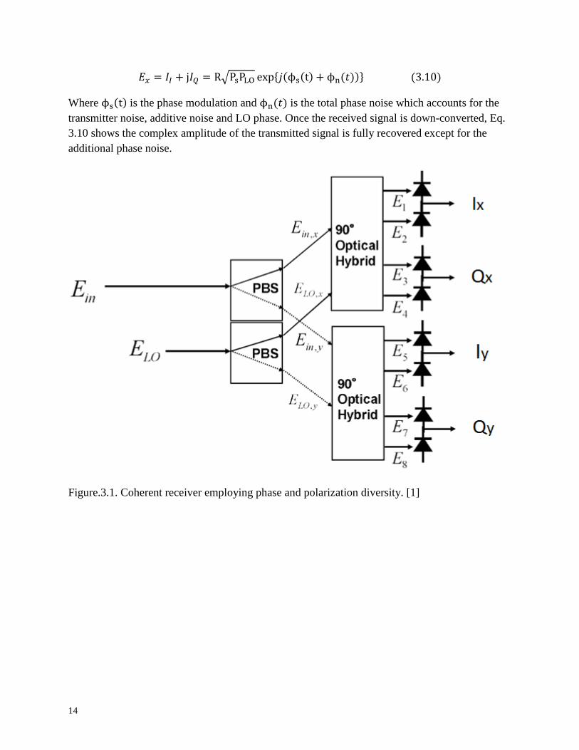
signal in two orthogonal polarizations. Fig.3.1 shows dual-polarization coherent receiver .The
incoming signal with arbitrary polarization and a LO signal are first split in two orthogonal
polarizations (these orthogonal polarizations not necessarily aligned with the original signal
polarizations) using a polarization beam splitter (PBS). The complex electric field in each
polarization is detected by letting the incoming data signal to interfere with the local oscillator
(LO) in an optical 90° hybrid followed by four pair of balanced detectors.
Let the incoming modulated signal in one polarization be:
Where As is the complex amplitude, ω0 is the angular frequency and ϕs is the signal phase. The
field of the local oscillator is:

13
Where ALO is the complex amplitude, ωLO is the angular frequency and ϕLO is the phase of the
LO. The complex amplitudes As and ALO are related to the signal powers Ps and LO power PLO
by:
Ps=| |
⁄ and PLO=
| |
⁄ .
The 900
optical hybrids shown in Fig 3.2 are used to detect both the in-phase and quadrature
components of the signal. A balanced detector is used to maximize the signal photocurrent and to
subtract DC components. The output optical fields from the 900
optical hybrids are given by:
The in-phase (I) and quadrature (Q) photocurrent differences after the balanced detectors are
given as:
| | | | √
| | | | √
Where is the intermediate frequency (IF) given by | |. when the value of
is higher than the modulation bandwidth of the optical signal the receiver termed as a
heterodyne coherent receiver and when it is exactly zero, the receiver termed as a homodyne
coherent receiver. We will focus on an intradyne coherent receiver in this paper. The
responsitivity, of a photodiode given by
Where e refers to electric charge, to the quantum efficiency of the photodiode, and h to
Planck’s constant. By combining Eq. 3.7 and 3.8 the complex amplitude on is given
by:
14
√ { }
Where is the phase modulation and is the total phase noise which accounts for the
transmitter noise, additive noise and LO phase. Once the received signal is down-converted, Eq.
3.10 shows the complex amplitude of the transmitted signal is fully recovered except for the
additional phase noise.
Figure.3.1. Coherent receiver employing phase and polarization diversity. [1]

15
Figure.3.2. 900 Optical Hybrid [1]
The outputs from the dual polarization coherent receiver are converted to digital data with an
analog digital convertor (ADC) and processed by the DSP circuit. The DSP circuit brings the
following benefits:
It is possible to synchronize the frequency and phase of transmitter with the LO light
without the need for a bulky and expensive phase locked loop (PLL).
As a result the LO laser requirement will be relaxed, and a commonly available WDM
laser can be used as free-running LO.
It is possible to track the continuously fluctuating state of polarization (SOP) of the
incoming signal.
Compensation of transmission impairments will be possible by distorting the digital
waveform
Figure 3.3 depicts the main sequence of operations in a typical DSP circuit. The 4-channel ADC
samples the in-phase and quadrature component of both polarizations, usually with a rate of 2
samples/symbol. Then the accumulated CD is compensated with a digital filter. After that, the
dual polarization signal is demultiplexed and the PMD is compensated using an adaptive filter in
a butterfly arrangement. After estimating the offset frequency between the transmitter and the
LO, the signal is down-converted. Then, the carrier phase is estimated. Finally, the symbol
estimation and decoding is performed. We now describe these blocks in more detail.
Figure.3.3. DSP block diagrams for dual polarization phase diversity receiver [1].

16
3.3 Chromatic Dispersion Compensation
CD is usually the main transmission impairment in a fiber-optic link. It is a phenomenon where
different spectral components of a signal propagate at different speeds along the length of the
fiber. If left uncompensated, it causes broadening to in signal pulses and thus significantly
reduces the data carrying capacity of the fiber. Traditionally, dispersion compensating fiber
(DCF) has been used to undo the dispersion in the fiber. However DCF incurs additional loss,
latency, and nonlinearity. CD compensation (CDC) using electronic signal processing removes
the need for these bulky and expensive optical components and offers additional flexibility
needed for future optical networks.
The propagation of a light pulse in optical fiber is described by the non-linear Schrodinger
equation (NLSE). [2]
| |
Where A stands for the field (could be the vector potential), γ for nonlinear coefficient,α for
attenuation coefficient and group veleocity dispersion (GVD).Neglecting attenuation and non-
linearity in equation 3.11,the effect of CD can be expressed as:
Where the dispersion coefficient D given by:
Solving (3.12) in the frequency domain gives:[3]
.
/
Thus, the effect of chromatic dispersion on the transmitted signal is modeled as an all-pass filter
with a quadratic phase response. Figure 3.4 shows the parabolic phase response of several
amounts of CD. The complex transfer function in frequency domain given by:
.
/

17
Figure.3.4. Phase response of dispersive fiber for several fiber length [4].
The effect of dispersion can be reversed or compensated by filtering with a tranfer function
.Such a filter can be realized by using an FIR filter,as shown in fig 3.5 [5].
With the coefficient given by the discrete inverse fourier transform of
∑
.
Figure.3.5 Schematic of an FIR filter for compensating chromatic dispersion

18
3.4 Polarization de-multiplexing
Transmitting two different signals at the same wavelength but in two orthogonal polarizations
(polarization multiplexing) enables doubling the number of transported bits while keeping the
same symbol rate compared to a single polarization transmission.[6].In the other way,for the
same bit rate requirement polarization multiplexing will half the clock speed and the symbol rate.
While the symbol rate reduction accounts to increased tolarance to inter sybol inteference (ISI),
two times lower clock speed translatea to a considerable power saving in the DSP core and
relaxing the ADC/DAC speed requirements. However the state of polarization (SOP) is not
preserved upon propagation on a standard single mode fiber unless polarization maintaining
fiber (PMF) is deployed for data transmision. Therefore, the receiver sees a linear combination of
vertical and horizontal signal in one polarization channel that lead to substantial crosstalk.
DSP is capable of estimating the jones matrix of the transmission channel and is able to undo the
polarization scrambling inside the fiber. There are two way of de-multiplexing polarizations: one
is by learning the channel matrix using a training sequence; the other is by using blind channel
equalization filter. The later being a more feasable solution as it does not need a prior knowledge
about the signal and will be examined in this section.
In addition to de-multiplexing the two polarizations, blind equalization is capable of
compensating other impairments like PMD, polarization dependent loss (PDL) and residual CD.
Its implementation is by using four FIR filters arranged as a butterfly structure (shown in fig
3.6).
The functionality of this filter structure is to perform inverse jones matrix of the channel, the
output is given by. [7]
Where h11, h12, h21, and h22 are N-tap FIR filters, with x (k) and y (k) representing a sliding
block of N input samples to which the filter is applied, such that,
. The coefficient of the filter tap is
updated by the well-known constant modulus algorithm (CMA).

19
Figure.3.6. Polarization de-multiplexing equalization filters architecture.
For the case of a polarization-division multiplexed quadrature phase shift keying (PDM-QPSK)
signal, the channel model and the CMA can be analyzed mathematically as follow.[7] Let us
express the transmitted signal in the form
[
] [
∑
∑
]
Where ,
√
√ -, T is the symbol period and p (t) is the pulse shape
After sampling the symbol synchronously eq. 3.18 gives:
[
] *
+
Where and
.

20
The main idea behind constant modulus algorithm is that the two polarization constellations
should have a constant modulus (as seen in eq. 3.19) because they are QPSK signals (except for
the transitions between symbols).
Neglecting polarization dependent loss (PDL), the channel can be modeled by a 2x2 unitary
matrix R.
0
1
Where corresponds for the azimuth and elevation angle of rotation respectively,
Thus, the received sample symbol is given by:
[
] [
] 0
1
Calculating the modulus of the signal, eq.3.21 gives:
[| |
| | ] [
]
Note that the total power in the two polarizations is constant by unitary rotation, with only the ratio
of power between the two polarizations changing. The output, x-polarization (X) and y-
polarization (Y) from the CMA is given by:
Where x (k) and y (k) is the input sample to the CMA and are the coefficients
of the four FIR filters and with an update algorithm given by:
Where μ is the step size, is the cost functions given by | | | | .

21
3.5 Frequency offset estimation
Ideally an intradyne coherent receiver requires lasers with narrow linewidth often on the order of
100 kHz, and very limited offset frequency between the transmitter laser and the local oscillator
(LO). However, it is desirable to use the commonly available WDM lasers to be able to reduce
the deployment cost.
Although the carrier phase estimation (to be discussed in the next section) will tolerate a laser
line width often of the order of 100MHz, the presence of an offset frequency will degrade the
performance of this algorithm. Commercially available tunable lasers have a frequency accuracy
of ±2.5 GHz over the life time. [8]. If left uncompensated the frequency offset causes a rotation
in constellation of a symbol, thus, the decoder will not be able to identify the symbol truthfully.
As a result, incorporating a separate frequency offset estimator circuit to the DSP core is
important. Depending on the type of modulation format used, many way of estimation can be
proposed. Straight-forward way estimation for QPSK format can be discussed. If the input signal
takes the form:
{ }
Where is the signal phase and T is the symbol period. A QPSK signal has four possible
phases {
}, such that the power of four operations can eliminate this signal phase.
Operating on consecutive samples gives:
{ ( )}
In [7], it was shown that, in the absence of additive noise, has a circular Gaussian
distribution, with mean due to the laser phase noise. And the probability density function
(pdf) for is:
{ }
Where, k corresponds to the linewidth of the laser. From the pdf, the offset frequency can be
estimated using maximum likelihood technique as: [7]
{∑
}
Where N is the number of samples used for the estimation.

22
3.6 Carrier phase estimation
Carrier synchronization in optical coherent systems can be achieved using digital phase
estimation techniques, allowing for a free running local oscillator without an optical phase-
locked loop [9].
Like the frequency estimation, carrier phase can be estimated using power of four operations for
QPSK modulation format. Taking the laser phase in to account, the input signal can be expressed
as:
{ }
Where the data phase, takes on four values {
} and is transmitter laser
phase in reference to the LO. When the sample is raised to the fourth power, we get:
{ }
The fourth power operation strips off the data phase ( { } ). The carrier phase
can then be estimated and subtracted from the phase the received signal to recover the data phase
as shown in fig 3.8.[5]
Figure.3.7 Feed-forward phase estimation algorithm for QPSK modulation.
The feed-forward algorithm is used only for ideal situation where there is no additive noise
present. In reality, the received signal will contain noise dominated by either amplified
spontaneous emission (ASE)-LO beat noise or shot noise of the LO. [5] The phase estimation
have to be modified to manage these noises, given as:[ 7].
{
∑
}
Where w[n] is a weighting function, which depends on the ratio of additive white Gaussian noise
to the laser phase noise. For a constant tap weighting function ,assuming the carrier phase is
constant over the sequence of sample, the variance of the phase estimation error due to additive
noise will be reduced by a factor 2N+1. However, the size of the weighting function has to be
limited as the filtering itself may introduce error since the carrier phase can’t be constant over a
large sequence of samples.

23
Since the phase estimate is forced in value in range
.there is a fourfold phase
ambiguity. It is important to differentially pre-code data to avoid cycle slips [5]. At the receiver,
differential decoding may also be implemented to reduce the impact of cyclic slips which can
create a catastrophic effect otherwise.
3.8 Simulation result
In addition to the theoretical analysis, the algorithms (i.e CMA, offset frequency estimation,
carrier phase estimation) are implemented in MATLAB to recover both QPSK and 16-QAM
modulation formats for the line rate of 120Gb/s. The electrical data signals each consist of
delayed copy of 215
pseudo-random binary sequences (PRBS). The noise of the optical
preamplifier was modeled as additive white Gaussian noise. The signal and local oscillator were
mixed by a 900 optical hybrid and the in-phase and quadrature channel of the signal is extracted
by balanced detectors.
Figure.3.9 shows a 30Gbaud PDM-QPSK signal recovery by using: CMA, frequency offset
estimation and carrier phase estimation algorithms. The received data constellation diagram is
shown in (a) for X-polarization. After running the CMA algorithm on the input samples, the
polarization separation is seen in the donut shape constellation in (b). After applying the phase
and frequency compensation algorithms the QPSK signal is recovered, Fig(c) shows the
recovered constellation for X-polarization.
Figure.3.8. PDM-QPSK Digital signal processing, (a) received symbol for X-pol (b) X-pol after
CMA polarization separation, with 100MHz offset frequency (c) X-pol after frequency and
phase compensation.(note: black star represent the ideal constellation points)
Similarly, it is also possible to recover 16-QAM with CMA algorithm, Fig.3.10 shows 15Gbaud
16-QAM signal recovery for two OSNR values: 12dB and 20dB (0.1nm-resolution bandwidth),
in the presence of 100MHz offset frequency. After the frequency and phase estimation the
recovered symbols have BER of 2x10⁻²
for 12dB OSNR, and BER of 3x10⁻⁵
for 20dB OSNR.

24
Figure.3.9. PDM-16QAM Digital signal processing, (i) for 12dB OSNR (0.1nm resolution
bandwidth) (ii) for 20dB OSNR (0.1nm bandwidth), (a) received symbol for X-pol (b) X-pol
after CMA polarization separation (c) X-pol after frequency and phase compensation.(note: red
star represent the ideal constellation points)

25
3.8 References
[1] K. Kikuchi, “Coherent Optical Communications : Historical,” History, pp. 1-42.
[2] Govind P.Agrawal. "Nonlinear Fiber Optics". Academic Press Second edition, 1995.
[3] M. Mussolin, “Digital Signal Processing Algorithms for High-Speed Coherent
Transmission in Optical Fibers,” Framework, 2010.
[4] G. Goldfarb and G. Li, “Coherent optical communications via digital signal processing,”
no. Dc, pp. 10-12.
[5] G. Li, “Recent advances in coherent optical communication,” Advances in Optics and
Photonics, vol. 1, no. 2, p. 279, Feb. 2009.
[6] C. Growth and O. Networks, “Next-generation Electro-Optics Technology with Coherent
Detection,” Technology.
[7] S. J. Savory, “Digital Coherent Optical Receivers: Algorithms and Subsystems,” IEEE
Journal of Selected Topics in Quantum Electronics, vol. 16, no. 5, pp. 1164-1179, Sep.
2010.
[8] I. Fatadin, S. J. Savory, and S. Member, “Compensation of Frequency Offset for 16-QAM
Optical Coherent Systems Using QPSK Partitioning,” Technology, vol. 23, no. 17, pp.
1246-1248, 2011.
[9] I. Fatadin, D. Ives, and S. J. Savory, “Laser Linewidth Tolerance for 16-QAM Coherent
Optical Systems Using QPSK Partitioning,” IEEE Photonics Technology Letters, vol. 22,
no. 9, pp. 631-633, May 2010.
[10] Mussolin, M., Forzati, M., Martensson, J., Carena, A., & Bosco, G. (2010). "DSP-based
compensation of non-linear impairments in 100 Gb/s PolMux QPSK". 2010 12th
International Conference on Transparent Optical Networks, 1, 1-4. Ieee.
doi:10.1109/ICTON.2010.5549084

26
Chapter 4
4. COMPENSATION OF PHOTONIC INTEGRATED CIRCUIT IMPERFECTION
4.1 Introduction
Most PIC imperfections can be compensated with DSP and/or optical element adjustments. The
imperfections can be in the transmitter or receiver, and likewise the DSP compensation
algorithms can be in the transmitter or receiver. In this chapter, some of the PIC imperfections
are analyzed and possible compensation mechanisms are proposed.
The DSP algorithms must be computationally efficient, because they occur in real time. The
number of two-variable multiplies must be minimized. They ideally should be able to be
pipelined.
First, limited extinction ratio could happen in the MZMs due to e.g., imperfect splitting of the 3-
dB couplers or unbalanced waveguide loss in the two arms of the MZM. In Sec. 4.2, a novel
compensation mechanism is proposed to improve the penalty due to finite extinction ratio.
Second, the effect of limited bandwidth and non-linearity is a pervasive imperfection in high-
speed transceivers and is discussed in Sec. 4.3. A high speed silicon modulator based on free
carrier plasma dispersion effect suffers from capacitance variation; in Sec. 4.4 a novel pre-
compensation scheme is described.
Finally, post compensation methods to correct I-Q phase error in the receiver or transmitter are
discussed in Secs. 4.5 and 4.6 respectively.
4.2 Compensation limited extinction ratio at MZM
One common non-ideality at the modulator is imperfect power splitting ratio in a balanced
MZM, leading to finite extinction ratios. When data transmission is considered, the finite
extinction ratio manifests itself in BER degradation. VOAs could be used to control the power
splitting in the MZMs, as perfect splitting is difficult to be achieved in realistic situations.
However, adding VOAs adds cost and complexity. In this section, novel electronic tuning and
pre-compensation mechanisms are proposed to compensate MZM finite extinction ratio. A
simulation for 16-QAM is performed.
a) Compensation by pre-distorting driver voltage
For a dual-parallel MZM with push-pull configuration, let the ratio of the amplitudes of the
electric fields from the two arms in the upper MZM is 1:γ2, in the lower MZM is 1:γ3 and the
outer MZM has splitting ratio of 1:γ1, as shown in Fig 4.1. In the ideal case, γ1 = γ2 = γ3 = 1

27
Figure.4.1. Dual Parallel MZM with unequal splitting ratio
If all the other parameters are perfect, and , the output field can be expressed as
{
(
)
(
)}
Assuming the DC bias voltages for both inner Mach-Zehnder are , the modulated optical
field is then expressed as:
{
( )
( )
} (4.2)
Where,
For a small drive voltage, after small angle approximation Eq.4.2 is reduced to:
,(
) (
)- (4.3)
The output signal encounters scaling and translation term in each quadrature due to the imperfect
splitting. However, if γ2 and γ3 are close to 1, the effect of scaling can be neglected (i.e
and Eq.4.3 is finally approximated as:

28
,(
) (
)- (4.4)
Driven with a small signal, the output optical field gives a linear combination of two electrical
drive voltages with an additional translation due to imperfect splitting. Imperfection at the in-
phase MZM causes back-ward translation to the quadrature channel while the imperfection at the
quadrature MZM causes a forward translation to the in-phase channel.
, by pre-distorting the
electrical driver signal, we will be able to get the desired optical signal from the imperfect
modulator.
For a dual parallel-MZM, we have two drive voltages. In order to generate a desired optical
signal with specified amplitude and phase at the output of modulator, first, two required
electrical drive voltages are back-calculated based on an inverse modulator transfer function.
Since
he the pre-distorted drive voltages will be:
{
(4.5)
Where, Vback1 and Vback1, the back calculated voltages for the ideal modulator
Note that, since the driver voltages are linearly proportional to data signals, a DC shift in the RF
voltage can give a similar compensation.
b) Compensation by scaling bias voltages
While changing the DC level of the drive voltage in accordance with splitting ratio works well to
compensate the imperfection, a more elegant way of compensation is proposed by adjusting the
bias voltages in the two MZMs.
To see the effect of scaling the bias voltages, let us modify the output of dual parallel-MZM by
adding scaling coefficients to bias voltages:
, (
) (
)-
(4.6)
Where, K1 and K2 is the scaling coefficient for the bias voltages
For a similar bias point (i.e.
), after small angle approximation,
Eq.4.6 can be expressed as:

29
,
- (4.7)
Scaling bias voltage in the in-phase (upper) MZM gives a linear translation in the in-phase
channel and scaling bias voltage in the quadrature (lower) MZM gives a linear translation in the
quadrature channel. Comparing Eqs.4.4 and 4.7, it is possible to compensate the amplitude
imbalance by scaling the bias voltages as:
{
(4.8)
The scaling in the upper MZM corresponds for the imbalance in the lower MZM and vice versa.
c) Simulation of a finite extinction ratio compensation
In addition to the theoretical analysis, the proposed method of pre-compensation was
numerically investigated using MATLAB. A 16QAM modulation format with 15Gbaud symbol
rate is used. The four multiplexed data signals each consist of 15-Gb/s 215
PRBS. At the
receiver, the noise of the optical preamplifier was modeled as additive white Gaussian noise. The
signal and local oscillator were mixed by a 900 optical hybrid and the in-phase and quadrature
channel of the signal is extracted by balanced detectors. Assuming and ,
Fig.4.2 (a) and (b) shows the constellation diagram with and without compensation for the case
when the splitting ration in both MZM is 1 to 0.8 (~19dB extinction ratio), and Fig (c) and (d)
for 1 to 0.65 splitting ratio in both MZM (~13.4dB extinction ratio).
Both Fig (a) and (c) show that limited extinction ratio causes linear translation along the real and
imaginary axes of the constellation diagram, and if left unattended will lead to substantial BER
degradation. It appears that the bias voltage scaling mechanism fully recovers the constellation
diagram for the case of ~19dB extinction ratio (Fig 4.2 (b)). However, because of the
approximation involved in the analytical analysis of the previous section and the assumption of
small signal modulation, the proposed method of compensation performs suboptimally for large
signal modulation or very low extinction ratio (i.e. less than 10dB) case. The compensation is not
perfect for the case of ~13.4dB (fig.4.2(d)) as compared to the case in (b).

30
Figure.4.2. Constellation diagrams of 16QAM using non-ideal MZM, (a) ~19dB extinction
ratio, not compensated (b) ~19dB extinction ratio after compensation (c) ~13.4 dB extinction
ratio, not compensated (d) ~13.4 dB extinction ratio after compensation . (Note the translation in
(a) and (c) from the desired * symbol).
In this section, a simple but novel method of compensating finite extinction ratio of a MZM is
presented. The method with bias voltage scaling will not add any computational burden to the
DSP circuit, yet it can reduce the number of VOA’s required in the modulator which will in turn
simplify the packaging and cost of photonic integrated circuit (PIC). The bias voltage defined in
Eq. 4.1 can be a very sensitive parameter to play with especially in silicon modulator where a
bias point can solely decide the speed of the modulator, however, in Si modulator there is a
separate thermooptic phase shifter in each arm of the MZM, a similar bias voltage scaling of the
phase shifters can do the job.[13]
4.3 Compensation of limited bandwidth and non-linearity
A high-speed optical transmitter comprises of a digital-to-analog convertor, a DSP, an electrical
driver and the actual phase modulators. Fig 4.3 shows the block diagram for a single
polarization transmitter. Encoding, waveform generation, DSP and DAC is executed in an ASIC
(application-specific integrated circuit). Common sources of limitations in such kinds of

31
transmitter are: non-linearity and non-flat frequency response of the DACs, drivers and optical
modulator and non-linearity in the phase modulator, driver and DACs. Non-linearity in the phase
modulator is unavoidable, however the presence of non-linearity in the driver and DAC will lead
to additional signal distortion if not compensated with the DSP. The DSP circuit is used to
implement a linear pre-emphasis filter and a non-linear equalizer to compensate bandwidth
limitation and nonlinearity of those devices. Figure 4.4 shows the sequential operation needed to be
performed in the ASIC.
Figure.4.3 Transmitter block-diagram
If the nonlinearity in the driver is neglected, the pre-emphasis filter can be computed by merging the
frequency responses of the DACs, Drivers and DP-MZM. And the back calculated driver voltages are
modified as:
Where are the back calculated driver voltage based on the desired complex
symbols. And F () and F-1() denote the Fourier transform and the inverse Fourier transform, respectively.
However, in the presence of driver nonlinearity, the compensation should follow the sequence in Fig 4.4.

32
Figure.4.4 Transmitter block-diagram involving linear filters and non-linear equalizers. [Partly
from 12]
At a given bit rate, PDM-16QAM signal has half the bandwidth requirement of PDM-QPSK. As
a result, 16-QAM has a more relaxed device requirement than the QPSK format in terms of
bandwidth for a given bit rate. A simulation is performed for 120-Gb/s polarization-division
multiplexed (PDM) quadrature phase-shift-keyed (QPSK) signal with I and Q components
consisting of delayed copies of 30-Gb/s 215
PRBS. Each quadrature data signal experiences
bandwidth limitation in the DAC, driver and modulator (e.g. 20GHz bandwidth is assumed for
DAC and driver, and 15GHz for the modulator). Figure 4.5 shows the simulation results
performed for a 15-dB OSNR 120-Gb/s signal. The bandwidth limitations severely degrade the
performance, unless it is compensated with a digital filter. A comparison between the phase
diagrams indicates that the pre-equalizing filter has eliminated the effect of limited bandwidth
and allows detection of the four phases of QPSK.

33
Figure 4.5 Phase diagrams and constellation diagrams without and with compensation of
bandwidth limitation in the transmitter for a 120-Gb/s PDM-QPSK signal.
4.4 Compensation of varying capacitance in silicon-modulator
(a) Si-modulator
Silicon-based devices like waveguides, modulators and detectors will enable high-speed
communication at a low cost, low power consumption and small footprint due to its
compatibility with mature silicon technology and the potential of combining electronics and
optics technology.
Silicon, unlike the traditional materials used for high-speed modulators, exhibits no linear
electro-optic effect and only very weak Kerr and Franz-Keldysh effects, and optical modulation
through the Pockels effects is not possible in silicon. [3]
High-speed modulation in silicon can instead be achieved through the plasma dispersion effect,
where a change in carrier concentration causes a change in absorption, and through the Kramer–
Kronig relations, a change in the refractive index. A carrier density variation can be reached by
carrier injection in a forward biased p-i-n diode, by accumulation in a metal–oxide–
semiconductor capacitor, or by depletion in a reverse biased p-n diode. The three types of Si
modulators are shown in Fig.4.6. (a) Shows a carrier-injection modulator. While this effect has
better modulation efficiency (VπL of 2.5 V-mm is possible), however due to its high injection

34
capacitance and slow free-carrier recombination achieving high speed modulation will be
difficult, it has typical speed below 5 GHz. Speeds up to 10 Gb/s have been achieved [2], but
require electronic pre-emphasis. (b) Shows a carrier depletion modulator. The effect is much
weaker (VπL of 25 V-mm is typical) but speeds in excess of 40 GHz are possible. 50-Gb/s
modulation has been reported [4]. Figure.4.6 (c) shows a metal-oxide-semiconductor (MOS)
modulator. The thin layer of oxide allows a larger carrier density change, thus, it has better
modulation efficiency than carrier-depletion in a reverse-biased pn junction (VπL of 2.5 V-mm is
possible). However, the speed of MOS-type modulator is limited by the high capacitance from
the thin oxide layer. [1, 2]
Figure.4.6 various type of Si modulator (a) carrier injection (b) carrier depletion (c) MOS [14]
Carrier depletion in reverse biased p-n diodes have an advantage on the operational speed since it
relies on the electric-field induced majority carrier dynamics. It is a widely used mechanism to
realize high-speed modulation in silicon. However, carrier depletion has low modulation
efficiency due to a relatively small overlap between the carrier depletion region and the optical
mode [3]. As a result there is are tradeoffs between speed, insertion loss and drive voltage of the
modulator.
The real and imaginary parts of the refractive index change of Si with free carrier distribution at
1.55μm wavelength are given by Soref’s relation [5].
Where Ne and Nh are the electron and hole densities, respectively. The hole density has a
stronger effect on the real part of the index change than the electron density yet the absorption is
approximately the same for hole and electron concentrations. For this reason, Si modulators are
typically designed to have a larger optical mode overlap with the p-doped region.
A typical plot of the phase response and normalized capacitance for varying driver voltage is
shown in Fig. 4.7. For a reverse bias voltage, the depletion width increases with the square root
of the applied voltage, thus the capacitance reduces as the voltage increases.

35
Figure.4.7. Relative phase shift and normalized capacitance at different phase shifter voltages.
[6]
As part of reducing the power consumption in an optical transponder, one of the main
performance requirements in the modulator is low RF power. Although, working at high
modulation efficiency region using a pre-emphasis driving signal may achieve this goal, there is
no fixed frequency response as the capacitance varies with the driving voltage.
(b) Pre-compensation
Device bandwidth limitation can be overcome by using a digital pre-compensation filter when
the frequency roll-off of the device is not too steep. Multilevel modulation in Si involves a
relatively large RF voltage swing. This results in a significant modulator capacitance change
during modulation. Thus there is not just one frequency response to use for the pre-compensating
filter. In other words, the impulse response of the modulator changes with drive voltage. In this
section a novel pre-compensation technique for a silicon depletion dual parallel MZM is
proposed.
Let the bias voltage at both arms of a MZM be zero, and assume there is an additional 180
degree phase shifter in the lower arm. If there is no capacitance variation in the modulator then
the output field from the dual parallel MZM can be expressed as:
{
(
)
(
)
}
36
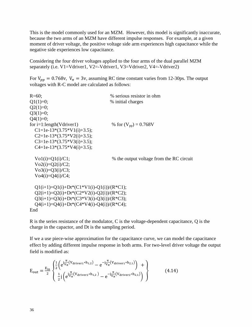
This is the model commonly used for an MZM. However, this model is significantly inaccurate,
because the two arms of an MZM have different impulse responses. For example, at a given
moment of driver voltage, the positive voltage side arm experiences high capacitance while the
negative side experiences low capacitance.
Considering the four driver voltages applied to the four arms of the dual parallel MZM
separately (i.e. V1=Vdriver1, V2=-Vdriver1, V3=Vdriver2, V4=-Vdriver2)
For , assuming RC time constant varies from 12-30ps. The output
voltages with R-C model are calculated as follows:
R=60; % serious resistor in ohm
Q1(1)=0; % initial charges
Q2(1)=0;
Q3(1)=0;
Q4(1)=0;
for i=1:length(Vdriver1) % for (Vpp) = 0.768V
C1=1e-13*(3.75*V1(i)+3.5);
C2=1e-13*(3.75*V2(i)+3.5);
C3=1e-13*(3.75*V3(i)+3.5);
C4=1e-13*(3.75*V4(i)+3.5);
Vo1(i)=Q1(i)/C1; % the output voltage from the RC circuit
Vo2(i)=Q2(i)/C2;
Vo3(i)=Q3(i)/C3;
Vo4(i)=Q4(i)/C4;
Q1(i+1)=Q1(i)+Dt*(C1*V1(i)-Q1(i))/(R*C1);
Q2(i+1)=Q2(i)+Dt*(C2*V2(i)-Q2(i))/(R*C2);
Q3(i+1)=Q3(i)+Dt*(C3*V3(i)-Q3(i))/(R*C3);
Q4(i+1)=Q4(i)+Dt*(C4*V4(i)-Q4(i))/(R*C4);
End
R is the series resistance of the modulator, C is the voltage-dependent capacitance, Q is the
charge in the capactor, and Dt is the sampling period.
If we a use piece-wise approximation for the capacitance curve, we can model the capacitance
effect by adding different impulse response in both arms. For two-level driver voltage the output
field is modified as:
{
(
( )
( )
)
(
( )
( )
)}

37
where “*” denotes convolution, and h is the local impulse response. When the first arm impulse
response is h1, the second arm will be h2 and vice versa.
For relatively small phase shift in the modulator, the above non-linear equation can be linearized
and approximated to get a resultant linear response.
After first order approximation and simplification, Eq. 4.14 gives:
,*
( )
+ *
( )
+ -
Figure.4.8. (a) shows a push-pull dual parallel MZM, and the corresponding linear filter
equivalence of a single MZM is shown in (b).
Figure.4.8. (a) Dual-Parallel MZM, (b) approximate linear filter equivalence for single MZM
When there is no capacitance variation, the expected small-signal modulated output field from
the DP-MZM can be expressed as:
,
-
Using the approximated linear response model, it is possible to pre-equalize the RF driver
voltage to overcome distortion induced by the non-linear bandwidth limitation of Si modulator.
For example, the two required pre-compensated drive voltages become as follows:
{ [ (
)
] }
{ [ (
)
] }
Where corresponds to the frequency responses of the modulator at the
positive and negative driver voltage respectively. In other words, we have discovered that we

38
can take the average of the impulse responses for the two diode conditions as the impulse
response to invert and use in the compensator.
Another possible way to track the modulator capacitance variation is to employ two drivers for a
single MZM, so that the two RF voltages can be distorted separately in the DSP circuit. In this
case two adaptive filters are used for a single quadrature. The filter coefficients are chosen
depending on the value of the driver voltage. For example, in 16-QAM modulation each driver
can have four different voltage levels, which means the equalizing filter for a single RF voltage
can have four different filter characteristics and chosen adaptively.
A simulation is performed for 15-Gbaud 16-QAM modulation, both static equalization (i.e based
on Eqs. 4.17 and 4.18) for a single-drive MZM and adaptive equalization for double drive MZM
is considered. Figure 4.9 (a) shows the piecewise approximation of the capacitance curve
employed in the compensation, (b) the pre-emphasis filter used for both type of equalization, the
black curve corresponds to the static equalizing filter, the other four curves for the adaptive
equalizing filter when two driver voltages used. For the simulation, the peak-to-peak driver
voltage (Vpp) is assumed to be 0.76V and the RC time constant varies from 18ps to 30ps linearly
with voltage.
The distorted constellation and closed eye diagram in Fig.4.10 (a) are due to the RC time
constant variation of the modulator. A single equalizing filter however gives a much better
performance, shown in (b). For the case of dual drive voltage the result of piecewise adaptive
equalizer is shown in (c).
Figure.4.9 (a) capacitance curve piecewise approximation (b) equalizing filters amplitude
response (black curve being for static equalizer)

39
Figure.4.10 constellation and eye diagram for 16QAM Si-modulator, (a) without pre-
compensation, (b) single driver MZM compensated with static average filter (b) double driver
MZM compensated with adaptive filter by piecewise capacitance approximation.
One can see that the piecewise filter adapting equalization does not give a better performance
despite its computational and hardware burden, whereas a single filter approach gives actually
slightly better performance with much more simple computation.
4.5 Compensation of imperfect hybrid phase and photodiodes responsivity mismatch
Imperfection of 900 hybrid and photodiode responsivity mismatch are important imperfection at
the phase diversity receiver. If left uncompensated, these imperfections will introduce gain and
phase imbalance between the in-phase and quadrature channels, commonly known as quadrature
imbalance.
Ideally, the I and Q channels of a phase-diversity receiver are orthogonal. However, the presence
of quadrature imbalance destroys the orthogonally between the two received channels and these
degrade the performance of the system. Several digital signal processing (DSP) algorithms have
been proposed so far to compensate quadrature imbalance for quadrature phase shift keying
(QPSK). [7-10]. Most of the quadrature imbalance compensation techniques have been based on
the Gram-Schmidt Orthogonalization procedure (GSOP).However, the impact of quadrature
imbalance compensation for M-QAM format and the effect of common mode rejection
ratio(CMMR) have not been analyzed yet. In [11], decision directed least-mean –square (DD-
LMS) adaptive filter method is proposed for 16-QAM case. In this section, a method of
compensating both amplitude and quadrature imbalance is proposed. A simulation for both
QPSK and 16QAM modulation format is performed to verify the proposed algorithm.

40
Referring to Fig. 3.1 of polarization diversity receiver, there are 8 photodiodes and 2 900 hybrids
for both polarizations.
Let the local oscillator split equally to both polarization and responsivity of the four photodiodes
for x-polarization be: r1, r2, r3 and r4. And let δ be the phase error in the 900 hybrid.
The output current from the four photodiodes will be:
| |
| |
| (
) |
| (
) |
Where the field from the LO, | | , with being the offset frequency between the
laser and LO and signal field | | .
After the balanced detector, the two output channels for x-polarization give,
| || | ( ) (| | | |
)
| || | (| | | |
)
The 90 degree hybrid phase error gives rise to phase error to the quadrature term, whereas,
unequal responsivity gives dc offset in other word reduces the common mode rejection ratio
(CMRR). For a constant-level modulation format like QPSK, the DC offset may be corrected by
subtracting the average levels from each channel. However, for a multi-level modulation format,
the DC offset depends on the signal, and hence the constellation diagram will be deformed.
(a) Quadrature Imbalance compensation for QPSK modulation
After subtracting the DC term from each channel, I and Q can be approximated as,
| || | ( )
| || |

41
Expressing in matrix form
[ ] | | [
] |
| [
]
Where,
| || | ( ) and | || | (
) are the expected output without phase error and responsivity imbalance.
Calculating inverse of the error matrix gives:
| | |
| |
|
As the phase error is expected to be small, the scaling term is neglected in the inverse
matrix. After compensation, I and Q will be nearly equal and orthogonal.
[
] | || | 0
( )
( )1 [
]
Next, the matrix coefficient is derived from the received sample signal,
Considering Eqs 4.25 and 4.26, multiplying I and Q gives:
| || |
{ }
After averaging over sufficient samples:
⟨ ⟩
| || |
The average power for in-phase and quadrature components is given by: ⟨ ⟩
| || | and ⟨ ⟩
| || |
.
Thus, the inverse matrix in equation 10 calculated as:
| | |
| |√
⟨ ⟩
⟨ ⟩
⟨ ⟩
⟨ ⟩ |

42
Given I and Q are the received samples, the resulting pair of equal and orthogonal signal denoted
by and computed as follows:
{ √
⟨ ⟩
⟨ ⟩
⟨ ⟩
⟨ ⟩
A simulation was performed for a QPSK signal with a 15-degree hybrid phase error and equal
photodiode responsivity. The received samples give a rhombic constellation diagram. The signal
is recovered into four orthogonal phase states using the method of Eq. 4.33. The result is shown
in fig.4.11.
Figure.4.11. Constellations diagram (a) with QI and frequency offset of 10MHz. (b) QI
compensated. (c) QI and frequency offset compensated. (Black dot represent the ideal
constellation symbol)
While the presence of offset frequency between the laser and LO causes rotation of the
constellation, the QI makes the shape elliptical (Fig.4.11a).The correlation method (Eq. 4.33)
correct the IQ mismatch and transforms the ellipse in to a circle (shown in fig.4.2b).After offset
frequency compensation, it is possible to identify and detect the signal as a QPSK signal as
shown in (c).
(b) Quadrature imbalance compensation for 16-QAM modulation
The effect of amplitude imbalance (e.g. due to responsivitiy inequality or due to imperfection in
the optical 90-degree hybrid) for 16-QAM modulation format is much more complex than
QPSK. Simple DC subtraction will not solve the amplitude imbalance problem, this is due to the
fact that some symbols in 16-QAM have different power levels (shown in Fig. 4.12)

43
Figure.4.12.16-QAM constellation points and QPSK partitioning
The compensation for the hybrid phase error will be the same as with the case of QPSK.
If r1 ≈ r2, r3 ≈ r4, Eq. 4.31 gives
⟨ ⟩
| || |
Where, | | √
However, in 16-QAM a small amplitude imbalance will give a distorted constellation diagram.
Considering Eqs 4.23 and 4.24, the translation term will result in non-uniform shift due to the
multi-level signal .
Fig. 4.13 is a simulation result for 16QAM in the presence of 15-degree hybrid phase error and
responsivity mismatch.
Figure 4.13.Constellation diagrams for 16-QAM signal with 15 degree hybrid phase error and
unequal photodiodes responsivity (a) without compensation (b) phase error compensated (c)
phase error compensated and channel DC value subtracted (* represent the ideal constellation
symbol)

44
In addition to non-orthogonality, the amplitude imbalance creates a non-even shift of the symbol
constellation point and non-uniform narrowing and spreading of the Gaussian noise (Fig.4.13a).
After compensating the non-orthogonality (b) using correlation method as Eq. 4.15, the problem
of amplitude imbalance can be clearly seen. (c) Shows the constellation diagram after subtracting
the average values from in-phase and Quadrature channels. It shows that a simple DC subtraction
will not fully remove the effect of amplitude imbalance. One way of reducing the effect of
amplitude imbalance for a higher modulation format is to increase power of the LO. This can be
seen in Eqs.4.23 and 4.24. When power of the LO is higher, the dominant DC term will be from
the LO and not the varying signal power.
4.6 Compensation of 90 degree phase error at MZM
The dual parallel MZM of Fig. 4.1 may experience error in the π/2 phase shifter. If it is not
corrected from the transmitter side, it will also contribute to quadrature imbalance in the received
signal and can be compensated in a similar manner with the previous section.
Let β be the error in π/2 phase shifter, the output field from the transmitter is then expressed as
* (
) +
Where
Expressing in terms of signal amplitude and phase (i.e
| |
| |
)
| |
Considering the offset frequency between the transmitter and LO, the balanced detector output
can be approximated as:
| || |
| || | ( )
Correlation between the two channels gives:
⟨ ⟩ | || |
Like the previous section, non-orthogonal I and Q the received samples can be transformed to
pair of orthogonal samples and as follows:

45
{
√⟨ ⟩
⟨ ⟩(
⟨ ⟩
⟨ ⟩)
⟨ ⟩
⟨ ⟩
√⟨ ⟩
⟨ ⟩
Where, ⟨ ⟩ and ⟨ ⟩ is the average power of in-phase and quadrature channel respectively.
Phase error at both transmitter and receiver in the presence of offset frequency gives an elliptical
and distorted constellation (Fig. 4.14 (a)). If the frequency offset is compensated but if there is
phase error at both the transmitter and receiver the constellation diagram looks rhombic as shown
in (b), whereas the constellation diagram takes on a non-rhombic shape if the phase error is only
at the transmitter or receiver as shown in (c). Like the hybrid phase error compensation, the
phase error of the transmitter is nicely compensated using Eq. 4.40. The recovered constellation
is shown in (d).
Eq.4.33 and 4.40 is valid to compensate a single quadrature phase error. However, phase error
could happen at both the transmitter and receiver or it could happen at both quadratures of either
end. A more generic solution is still to be devised to compensate all at once.

46
Figure.4.14 Constellation diagram illustrating the effect of 90 degree phase error at MZM and
hybrid detector (a) with 100MHz offset frequency ,120 phase error at transmitter and receiver (b)
with offset frequency compensated (c) with offset frequency compensated and in the presence of
120 phase error at transmitter (d) both offset frequency and phase error compensated.(note: a
closer look at the shapes of the constellation, (b) looks like rhombic whereas (c) looks like
parallelogram).
An efficient method for compensation of 90 degree phase shifter error at the MZM for the case
of 16-QAM modulation format is proposed. The effectiveness of the algorithm is also verified
with numerical simulations.

47
4.7 References
[1] Liu, A., and others, (2007). “Recent advances in high speed silicon optical modulator".
Proceedings of SPIE, 6477, 647710-647710-9. Spie. doi:10.1117/12.703127
[2] Dong, P., Chen, L., Chen, Y.-kai, Labs, B., & Road, H. (2012).” silicon Mach-Zehnder
modulators”, 20(6), 6163-6169.
[3] Yu, H., Bogaerts, W., & De Keersgieter, A. (2010). “Optimization of Ion Implantation
Condition for Depletion-Type Silicon Optical Modulators”. IEEE Journal of Quantum
Electronics, 46(12), 1763-1768. doi:10.1109/JQE.2010.2067206
[4] D. J. Thomson,and others , “50-Gb/s Silicon Optical Modulator," IEEE Photon. Tech. Lett.
24, 234{236 (2012).
[5] R. Soref and B. Bennett, “Electrooptical effect in silicon," IEEE Journal of Quantum
Electronics 23, 123{129 (1987).
[6] Liow, T.-yang, Ang, K.-wee, Fang, Q., & Song, J.-feng. (2010). “Silicon Modulators and
Germanium Photodetectors on SOI: Monolithic Integration, Compatibility, and
Performance Optimization” IEEE Journal of Selected Topics in Quantum Electronics,
16(1), 307-315. doi:10.1109/JSTQE.2009.2028657
[7] Thompson, B. J. (1981). “Correction of I and Q Errors in a coherent processor”, Ieee
Transactions On Aerospace and Electronic Systems, (1), 131-137.
[8] Fatadin, I., Savory, S. J., & Ives, D. (2008). Compensation of Quadrature Imbalance in an
Optical QPSK Coherent Receiver. October, 20(20), 1733-1735.
[9] Petrou, C. S., Vgenis, a., Roudas, I., & Raptis, L. (2009). Quadrature Imbalance
Compensation for PDM QPSK Coherent Optical Systems. IEEE Photonics Technology Letters,
21(24), 1876-1878. doi:10.1109/LPT.2009.2034750
[10] Fatadin, I., & Savory, S. J. (2010). DSP Techniques for 16-QAM Coherent Optical.
Quantum, 2(4), 22-23.
[11] Md.Saifuddin Faruk Compensation of Quadrature Imbalance in an Optical 16-QAM Digital
Coherent Receiver. Computer Engineering, (Iccit), 22-24
[12] Hoshida, T., Nakashima, H., Tanimura, T., Akiyama, Y., Rasmussen, J. C., & Limited, F.
(2012). “Digital compensation techniques for device characteristics imperfections in optical
transmission”.
[13] Christian.Rasmussen, Christopher R. Doerr, “discussion”,2012
[14] R. Nagarajan, C. R. Doerr, and F. Kish, “Semiconductor Photonic Integrated Circuit
Transmitters and Receivers,” to appear in Optical Fiber Telecommunications VI.

48
Chapter 5
5. EXPERIMENTAL RESULT AND ANALYSIS
5.1 Introduction
To verify the validity of the algorithms discussed in Chap. 3 for a coherent receiver, offline DSP
post processing of real transmission data is performed. Using a DSP algorithm, a PDM-QPSK
signal is recovered from the data captured from a 100-Gb/s coherent system. The symbol rate is
30Gbaud, the system employing 20% overhead for forward-error correction (FEC). In addition,
BER degradation caused by nonlinearity in the detector response due to the saturation of the
transimpedance amplifier (TIA) is measured. A nonlinear equalization algorithm is applied to
compensate for this imperfection and hence improve the BER.
5.2 Experimental set up
The experimental setup for back-to-back measurement is shown in Fig. 5.1. An amplified
spontaneous emission noise source is used to obtain different OSNR levels. The transmitter
generates two orthogonal QPSK signals, by using an electrical data pattern of 215
-1 PRBS. Each
electrical channel has a data rate of 30Gb/s yielding a single-channel line rate of 120 Gb/s. At the
receiver, the signal is combined with a free-running LO in a polarization diversity 90-degree
hybrid followed by four balanced detectors. The four signal components (Ix, Qx, Iy, Qy) are
sampled with a real-time scope. Off-line data processing was subsequently performed using
algorithms implemented in MATLAB. The sampling rate of the scope is 50Gsample/s. The
samples are up-sampled to two samples per symbol resulting in 60Gsample/s.
4 x 12-tap adaptive butterfly-structured FIR filters are applied on the up-sampled data to realize
polarization separation and equalization of the signal. These filters are adapted with a CMA
algorithm. Once the CMA converges, the received signals are separated into two orthogonal
polarizations. Later on, the frequency offset between the transmitter laser and LO laser is
estimated with a 100-sample window. Eventually, the carrier phase is estimated with an 8-tap
feed-forward algorithm.
To avoid the problem of cycle slip (discussed in Sec. 3.6), differential encoding is employed at
the transmitter. Likewise, after thresholding the recovered constellation, the decision is
differentially decoded. Finally the bit errors are counted to evaluate the performance of the post-
processing algorithms. No FEC operations were employed, i.e., the BER reported here is raw.

49
Figure.5.1. Offline processing test set up
5.3 Result and analysis
Figure.5.2 shows a QPSK signal recovery through a sequence of DSP algorithms. The received
data constellation diagram without DSP is shown in (a) for X-polarization. After running the
CMA algorithm on the input samples with convergence parameter μ chosen to be 10-3
, the
polarization separation is seen in (b). At this stage, it is noticed that the shape of the constellation
looks like a donut as the carrier phase and frequency offset is yet to be compensated. Then, the
offset frequency is estimated and removed using the method mentioned in Eq. 3.32. Finally, a
symbol by symbol laser phase tracking (Eq. 3.35) with constant weighting function is applied.
Figures (c) and (d) show the final recovered QPSK signal for X polarization and Y polarization,
respectively, after the phase and frequency compensation.

50
Figure.5.2 Constellation diagrams illustrating sequence of DSP processing on the real PDM-
QPSK signal. 120Gb/s, 20dB OSNR, (a) Input X-pol (b) X-Pol after CMA (c) X-pol after phase
and offset frequency compensation (d) Y-pol after phase and offset frequency compensation.
It is demonstrated that the PDM-QPSK signal is recovered for different OSNR values (0.1-nm
reference bandwidth). Figure 5.3 shows the back-to-back bit error ratio (BER) performance for
both polarizations.

51
Figure.5.3 BER performance at 30Gbaud: dual-polarization 120Gb/s QPSK
Figure.5.4. BER versus LO power for 0dBm signal power. The green square after nonlinear
equalization is for 15.5 dBm LO power.
We furthermore studied data corruption due to saturation in the TIA response. A BER curve for
one of the polarizations for different LO powers is shown in Figure.5.4. Significant degradation
is seen once the TIA reaches saturation. (e.g. 15.5 dBm LO power results in BER~10-1
). After
the application of some nonlinear equalization to the received symbols, with cubic function to
the four channels given as:

52
{
(5.1)
Where, are the input samples, k is optimization coefficient and
are the equalized samples
The BER is improved by about two orders of magnitude (from 10-1
to ~10-3
).

53
Chapter 6
6. CONCLUSION AND RECOMMENDATIONS
6.1 conclusions
In this thesis, DSP algorithms used in current optical coherent communication links are studied.
Some of the most common PIC imperfections are analyzed and some mitigation techniques are
proposed.
The proposed compensation mechanisms for PIC imperfections include:
Tuning the bias or phase shifter voltage of the modulator to compensate the effect of
limited modulator extinction ratio
Electronic pre-distortion of the modulator driving voltage to compensate imperfections
associated with bandwidth limits and nonlinearities of the devices at the transmitter
Electronic pre-distortion of the modulator driving voltage to compensate the effect of
capacitance variation in high-speed silicon modulators
Post compensation at the receiver to correct I-Q phase error in the receiver or transmitter
Post compensation at the receiver to correct for nonlinearity in the receiver
DSP algorithms used for a coherent receiver are verified by applying a post-processing algorithm
on real data experimentally captured from a 100-Gb/s coherent optical transmission setup.
Successful recovery of a PDM-QPSK signal is demonstrated, and the BER is measured. In
addition, it is shown that nonlinear equalization algorithms can be employed to improve the BER
induced by nonlinear behaviors in devices either at transmitter or receiver side. This is verified
by applying a nonlinear equalization to the received symbols in order to compensate for
imperfections caused by saturation in the TIA circuit at the detector. A two-order-of-magnitude
improvement in the BER is achieved with this technique. Optimized algorithms can lead to
further BER improvements.
Despite the fact that DSP promises a high potential for mitigating PIC imperfections, future
progress must be concurrently made to make the algorithms efficient both in energy and in
computation. In addition, more robust and informative performance measures for an optical data
link will be required to make the DSP techniques more effective. For instance, BER
measurements or constellation diagrams can be ineffective to isolate the root causes as an
imperfection can practically involve complex origins.

54
6.2. Future work
Future work would involve the study of other important PIC imperfections such as those
associated with nonlinearities in photodiodes, limited polarization extinction ratios, and electrical
crosstalk. Moreover, the computational complexity of all the proposed algorithms needs to be
evaluated and optimizations have to be done to make them suitable for real time operations.
While it has been numerically demonstrated that DSP can be used to compensate PIC
imperfection, it is important to see how the DSP algorithms perform experimentally on the real
PIC.
Finally, the proposed algorithms need to be employed in an actual ASIC and be measured in real
time.