digital signal processing chap 8. discrete fourier...
TRANSCRIPT
Digital Signal Processing
Chap 8.
Discrete Fourier Transform
Chang-Su Kim

Definition

Definition
• 𝑁-point input signal 𝑥 𝑛 , 0 ≤ 𝑛 ≤ 𝑁 − 1
• Discrete Fourier Transform (DFT)
𝑋 𝑘 =
𝑛=0
𝑁−1
𝑥 𝑛 𝑒−𝑗2𝜋𝑘𝑛/𝑁 =
𝑛=0
𝑁−1
𝑥 𝑛 𝑊𝑁𝑘𝑛
for each 0 ≤ 𝑘 ≤ 𝑁 − 1, where 𝑊𝑁 = 𝑒−𝑗2𝜋
𝑁
• Inverse Discrete Fourier Transform (IDFT)
𝑥 𝑛 =1
𝑁
𝑘=0
𝑁−1
𝑋 𝑘 𝑒𝑗2𝜋𝑘𝑛/𝑁 =1
𝑁
𝑘=0
𝑁−1
𝑋 𝑘 𝑊𝑁−𝑘𝑛
for each 0 ≤ 𝑛 ≤ 𝑁 − 1

DFT is a Lossless Representation
• 𝑥 𝑛DFT
𝑋 𝑘IDFT
𝑦[𝑛], then 𝑦 𝑛 = 𝑥[𝑛]

Examples
• Ex 1) Consider the length-𝑁 sequence
𝑥 𝑛 = 1, 𝑛 = 00, 1 ≤ 𝑛 ≤ 𝑁 − 1
• Ex 2) Consider the length-𝑁 sequence
𝑔 𝑛 = cos2𝜋𝑟𝑛
𝑁
where 𝑟 is an integer between 1 and 𝑁 − 1

Matrix Representation of DFT
1 2 1
2 4 2( 1)
1 2( 1) ( 1)( 1)
or
1 1 1 1[0] [0]
1[1] [1]
1[2] [2]
1[ 1] [ 1]
N N N
N
N N N
N
N N N
N N N N
N N N
X x
W W WX x
W W WX x
W W WX N x N
X W x
Forward Transform

Matrix Representation of DFT
1
1 2 ( 1)
2 4 2( 1)
( 1) 2( 1) ( 1)( 1)
or
1 1 1 1[0] [0]
1[1] [1]1
1[2] [2]
1[ 1] [ 1]
N N N
N
N N N
N
N N N
N N N N
N N N
x X
W W Wx X
W W Wx XN
W W Wx N X N
x W X
Inverse Transform
1 *1N N
N
W W
• DFT can be interpreted as an invertible matrix
• The forward and inverse matrices are related by

Relationships between
DFT and DTFT

DFT and DTFT
• Let 𝑋 𝑒𝑗𝜔 denote the DTFT of 𝑥 𝑛 , 0 ≤ 𝑛 ≤ 𝑁 − 1, then
𝑋 𝑘 = 𝑋 𝑒𝑗𝜔 𝜔=2𝜋𝑘/𝑁
– 𝑋[𝑘] is the set of frequency samples of the DFTF 𝑋 𝑒𝑗𝜔 of the
length-𝑁 sequence at 𝑁 equally spaced frequencies
– Thus, 𝑋 𝑘 is also a frequency-domain representation of the
sequence 𝑥[𝑛]

DFT and DTFT
• DTFT of a finite-length
sequence can be plotted
with high precision using
DFT
• Ex) DTFT of 𝑥 𝑛 =
cos6𝜋𝑛
16, 0 ≤ 𝑛 ≤ 15

Circular Convolution
Theorem
Extensions are Periodic
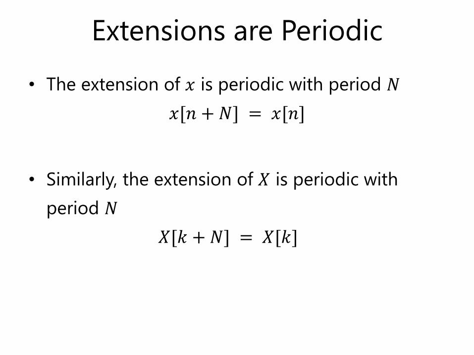
• The extension of 𝑥 is periodic with period 𝑁
𝑥[𝑛 + 𝑁] = 𝑥[𝑛]
• Similarly, the extension of 𝑋 is periodic with
period 𝑁
𝑋[𝑘 + 𝑁] = 𝑋[𝑘]
Extensions are Periodic
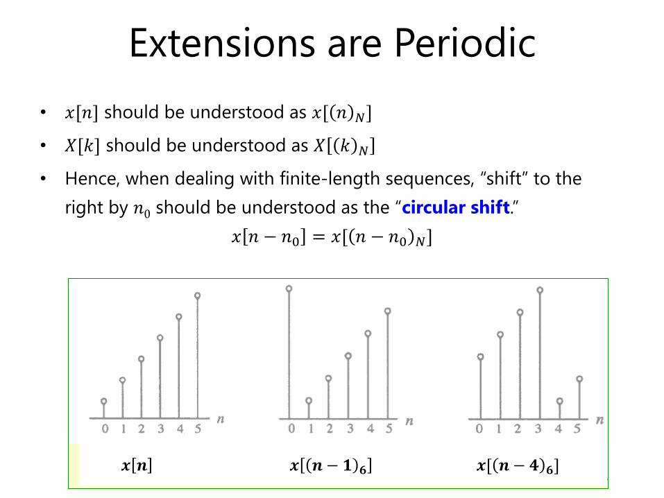
• 𝑥[𝑛] should be understood as 𝑥[ 𝑛 𝑁]
• 𝑋[𝑘] should be understood as 𝑋 𝑘 𝑁
• Hence, when dealing with finite-length sequences, “shift” to the
right by 𝑛0 should be understood as the “circular shift.”
𝑥 𝑛 − 𝑛0 = 𝑥[ 𝑛 − 𝑛0 𝑁]
𝒙 𝒏 𝒙 𝒏 − 𝟏 𝟔 𝒙[ 𝒏 − 𝟒 𝟔]

Circular Shift
• A circular shift of an N-
point sequence is
equivalent to a linear shift
of its periodic extension

Circular Shift
• A circular shift of an N-
point sequence is
equivalent to a linear shift
of its periodic extension
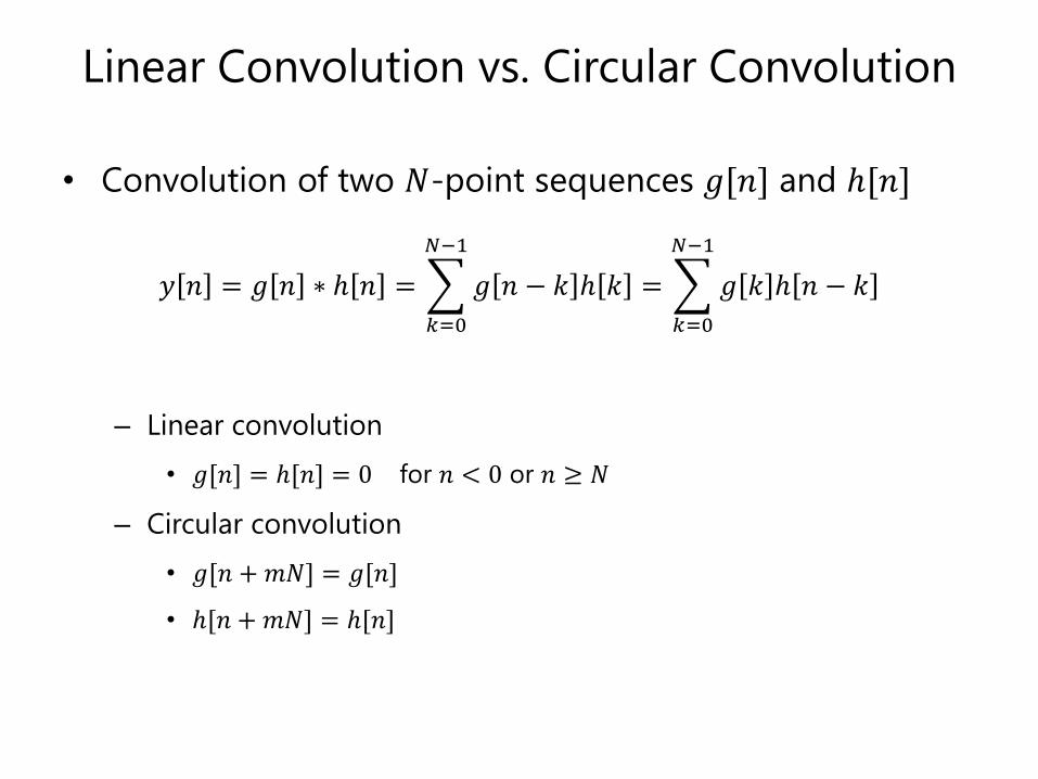
Linear Convolution vs. Circular Convolution
• Convolution of two 𝑁-point sequences 𝑔[𝑛] and ℎ[𝑛]
𝑦 𝑛 = 𝑔 𝑛 ∗ ℎ 𝑛 =
𝑘=0
𝑁−1
𝑔 𝑛 − 𝑘 ℎ 𝑘 =
𝑘=0
𝑁−1
𝑔 𝑘 ℎ 𝑛 − 𝑘
– Linear convolution
• 𝑔[𝑛] = ℎ[𝑛] = 0 for 𝑛 < 0 or 𝑛 ≥ 𝑁
– Circular convolution
• 𝑔[𝑛 + 𝑚𝑁] = 𝑔[𝑛]
• ℎ[𝑛 + 𝑚𝑁] = ℎ[𝑛]
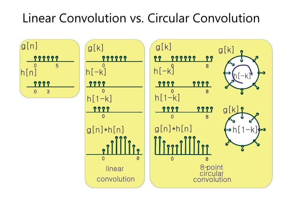
Linear Convolution vs. Circular Convolution
8-pointcircularconvolution
linear
convolution
0
0
0
0 8
0
0 3
5 0
0
0
0
8
8
8
8
h(-x)
)
h(1-x)
8-pointcircularconvolution
linear
convolution
0
0
0
0 8
0
0 3
5 0
0
0
0
8
8
8
8
0
0
0
0 8
0
0
0
0 8
0
0 3
5
g[n]
g[n]*h[n] g[n]*h[n]
g[ ]k g[ ]k g[ ]k
g[ ]k
h -k[ ] h -k[ ]
h 1-k[ ] h 1-k[ ]
h[n]0
0 3
5 0
0
0
0
8
8
8
8
0
0
0
0
8
8
8
8
h(-x
h(1-x)
h -k[ ]
h 1-k[ ]

𝑁-Point Circular Convolution
𝑦 𝑛 = 𝑔 𝑛 ⊛ ℎ 𝑛 =
𝑘=0
𝑁−1
𝑔 𝑛 − 𝑘 𝑁 ℎ 𝑘 =
𝑘=0
𝑁−1
𝑔 𝑘 ℎ 𝑛 − 𝑘 𝑘
• Ex) Circularly convolve {2, 1, 2, 1} and {1, 2, 3, 4}

Using Circular Convolution to Obtain Linear
Convolution
• Conditions
– 𝑔[𝑛]: 𝑴-point sequence, 𝑔[𝑛] = 0 for 𝑛 < 0 or 𝑛 > 𝑀 − 1
– ℎ[𝑛]: 𝑵-point sequence, ℎ[𝑛] = 0 for 𝑛 < 0 or 𝑛 > 𝑁 − 1
– The linear convolution of 𝒈[𝒏] and 𝒉[𝒏] generates (𝑴 + 𝑵 − 𝟏)-point
sequence, 𝑔[𝑛] ∗ ℎ[𝑛] = 0 for 𝑛 < 0 or 𝑛 > 𝑀 + 𝑁 − 2
• Procedures
1. Zero padding 𝑔[𝑛] and ℎ[𝑛] to yield (𝑀 + 𝑁 − 1)-point sequence
𝑔𝑝[𝑛] and ℎ𝑝[𝑛].
2. Obtain (𝑀 + 𝑁 − 1)-point circular convolution of 𝑔𝑝[𝑛] and ℎ𝑝[𝑛]
3. Result of Step 2 is equivalent to the linear convolution of 𝑔[𝑛] and ℎ[𝑛]

Circular Convolution Theorem
• 𝑔[𝑛] ⊛ ℎ 𝑛DFT
𝐺 𝑘 𝐻[𝑘]

Additional Properties of
DFT

Real-Valued Sequence 𝑥[𝑛]
• 𝑋∗[𝑘] = 𝑋[−𝑘] = 𝑋[𝑁 − 𝑘]

Time Reversal
• 𝑥 −𝑛 𝑁 = 𝑥 𝑁 − 𝑛DFT
𝑋 −𝑘 𝑁 = 𝑋 𝑁 − 𝑘
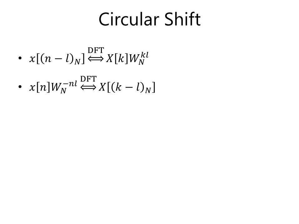
Circular Shift
• 𝑥 𝑛 − 𝑙 𝑁
DFT𝑋 𝑘 𝑊𝑁
𝑘𝑙
• 𝑥 𝑛 𝑊𝑁−𝑛𝑙
DFT𝑋 𝑘 − 𝑙 𝑁

Multiplication of Two Sequences
• 𝑥 𝑛 𝑦 𝑛DFT 1
𝑁𝑋 𝑘 ⊛ 𝑌[𝑘]

Parseval’s Theorem
• 𝑛=1𝑁−1 |𝑥 𝑛 |2 =
1
𝑁 𝑘=1
𝑁−1 |𝑋 𝑘 |2