digital signal processing - biher · system the solutions are obtained in real time ... notation...

Digital Signal Processing

BEC505

Chapter 1: Introduction

What is a Signal?

Anything which carries information is a signal. e.g. human voice, chirping of birds, smoke signals,

gestures (sign language), fragrances of the flowers.

Many of our body functions are regulated by chemical signals, blind people use sense of touch. Bees

communicate by their dancing pattern.

Modern high speed signals are: voltage changer in a telephone wire, the electromagnetic field

emanating from a transmitting antenna,variation of light intensity in an optical fiber.

Thus we see that there is an almost endless variety of signals and a large number of ways in which

signals are carried from on place to another place.

Signals: The Mathematical Way

A signal is a real (or complex) valued function of one or more real variable(s).When the function

depends on a single variable, the signal is said to be one-dimensional and when the function depends on

two or more variables, the signal is said to be multidimensional.

Examples of a one dimensional signal: A speech signal, daily maximum temperature, annual rainfall at a

place

An example of a two dimensional signal: An image is a two dimensional signal, vertical and horizontal

coordinates representing the two dimensions.

Four Dimensions: Our physical world is four dimensional(three spatial and one temporal).

What is Signal processing?

Processing means operating in some fashion on a signal to extract some useful information e.g. we use

our ears as input device and then auditory pathways in the brain to extract the information. The signal is

processed by a system. In the example mentioned above the system is biological in nature.

The signal processor may be an electronic system, a mechanical system or even it might be a computer

program.

Analog versus digital signal processing

The signal processing operations involved in many applications like communication systems, control

systems, instrumentation, biomedical signal processing etc can be implemented in two different ways

Analog or continuous time method

Digital or discrete time method..

Analog signal processing

Uses analog circuit elements such as resistors, capacitors, transistors, diodes etc

Based on natural ability of the analog system to solve differential equations that describe a physical

system

The solutions are obtained in real time...

Digital signal processing

The word digital in digital signal processing means that the processing is done either by a digital

hardware or by a digital computer.

Relies on numerical calculations

The method may or may not give results in real time..

The advantages of digital approach over analog approach

Flexibility: Same hardware can be used to do various kind of signal pr

case of analog signal processing one has to design a system for each kind of operation

Repeatability: The same signal processing operation can be repeated again and again giving same

results, while in analog systems there ma

supply voltage.

The choice of choosing between analog or digital signal processing depends on the application. One has

to compare design time,size and thecost of the implementation.

Classification of signals

We use the term signal to mean a real or complex valued function of real variable(s) and denote the

signal by x(t)

The variable t is called independent variable and the value x of t as dependent variable.

When t takes a vales in a countable set t

t ε {0, T, 2T, 3T, 4T,...}

t ε {....-1, 0 ,1,...}

t ε {1/2, 3/2, 5/2, 7/2,...}

For convenience of presentation we use the notation x[n] to denote dis

dependent and independent variables take values in countable sets (two sets can be quite different) the

signal is called Digital Signal.

When both the dependent and independent variable take value in continous set interval,

called an Analog Signal.

Notation:

When we write x(t) it has two meanings. One is value of x at time t and the other is the pairs (x(t), t)

allowable value of t. By signal we mean the second interpretation.

Notation for continous time signal

{x(t)} denotes the continuous time signal. Here {x(t)} is short notation for {x(t), t ε I } where I is the set in

which t takes the value.

Notation for discrete time signal

Similarly for discrete time signal we will use the notation {x(t)}, where {x(t)}

Note that in {x(t)} and {x[n]} are dummy variables ie. {x[n]} and {x[t]} refer to the same signal. Some

books use the notation x [.] to denote {x[n]} and x[n] to denote value of x at time n.

{x(t)} refers to the whole waveform,while x[n] refers to a particular value.

Most of the books do not make this distinction clean and use x[n] to denote signal and x[n0] to denote a

particular value.

Discrete Time Signal Processing and Digital Signal Processing

When we use digital computers to do processing we are doing digital signal processing. But most of the

theory is for discrete time signal processing where dependent variable generally is continuous. This is

because of the mathematical simplicity of discrete time signal proces

to implement this as closely as possible. Thus what we study is mostly discrete time signal processing

and what is really implemented is digital signal processing.

Elementary Signals

There are several elementary signals that occur prominently in the study of digital signals and digital

signal processing.

(a) UNIT SAMPLE SEQUENCE:

The advantages of digital approach over analog approach

Flexibility: Same hardware can be used to do various kind of signal processing operation,while in the

case of analog signal processing one has to design a system for each kind of operation


results, while in analog systems there may be parameter variation due to change in temperature or


to compare design time,size and thecost of the implementation.



When t takes a vales in a countable set the signal is called a discrete time signal. For example

1, 0 ,1,...}

For convenience of presentation we use the notation x[n] to denote discrete time signal. When both the


When both the dependent and independent variable take value in continous set interval,


allowable value of t. By signal we mean the second interpretation.


Similarly for discrete time signal we will use the notation {x(t)}, where {x(t)} is short for {x(t), n ε I }.


books use the notation x [.] to denote {x[n]} and x[n] to denote value of x at time n.

rm,while x[n] refers to a particular value.


Discrete Time Signal Processing and Digital Signal Processing

computers to do processing we are doing digital signal processing. But most of the


because of the mathematical simplicity of discrete time signal processing. Digital Signal Processing tries


and what is really implemented is digital signal processing.

signals that occur prominently in the study of digital signals and digital

ocessing operation,while in the


y be parameter variation due to change in temperature or




he signal is called a discrete time signal. For example

crete time signal. When both the


When both the dependent and independent variable take value in continous set interval, the signal is



is short for {x(t), n ε I }.



computers to do processing we are doing digital signal processing. But most of the


sing. Digital Signal Processing tries


signals that occur prominently in the study of digital signals and digital

Defined by

Graphically this is as shown below.

Unit sample sequence is also known as

This plays role akin to the impulse function

is purely a mathematical construct while in discrete time we can actually generate the

sequence.

(b) UNIT STEP SEQUENCE:

Defined by :

Graphically this is as shown below

(c) EXPONENTIALSEQUENCE:

The complex exponential signal or sequence {x[n]}

where C and α are, in general, complex numbers.

Note that by writing α = eβ , we can write the exponential sequence as

Real exponential signals:

: If C and are real, we can have one of the several type of behavior illustrated below

Unit sample sequence is also known as impulse sequence.

role akin to the impulse function of continous time. The continues time impulse

is purely a mathematical construct while in discrete time we can actually generate the

The complex exponential signal or sequence {x[n]} is defined by x[n] = C αn

and α are, in general, complex numbers.

, we can write the exponential sequence as x[n] = c eβn

are real, we can have one of the several type of behavior illustrated below

of continous time. The continues time impulse

is purely a mathematical construct while in discrete time we can actually generate the impulse

are real, we can have one of the several type of behavior illustrated below

For |α| > 1

|α| < 1

For α > 1

α < 1 sign of terms in {x[n]}

(d)SINUSOIDAL SIGNAL:

The sinusoidal signal {x[n]} is defined by

Euler's relation allows us to relate complex exponentials and sinusoids as

and

The general discrete time complex exponential can be written in terms of real exponential and

sinusiodal signals.

Specifically if we write C and α in polar form

Thus for |α| = 1 , the real and imaginary part

|α| < 1, they correspond to sinusoidal sequence multiplied by a decaying exponential,

|α| > 1 , they correspond to sinusiodal sequence multiplied by a growing exponential

Generating Signals with MATLAB

MATLAB, acronym for MATrix LABoratory has become a very popular software environment for

complex based study of signals and systems. Here we give some sample programmes

elementary signals discussed above. For details one should consider MATLAB manual or read help

files.

In MATLAB, ones(M,N) is an M-

zeros. We may use those two matrices to generate

magnitude of the signals grows exponentially,

|α| < 1 It is decaying exponential.

all terms of {x[n]} have same sign,

sign of terms in {x[n]} alternates.

is defined by

Euler's relation allows us to relate complex exponentials and sinusoids as


and α in polar form and then

, the real and imaginary parts of a complex exponential sequence are sinusoidal.


|α| > 1 , they correspond to sinusiodal sequence multiplied by a growing exponential


complex based study of signals and systems. Here we give some sample programmes


-by-N matrix of ones, and zeros(M,N) is an M-

We may use those two matrices to generate impulse and step sequence.

magnitude of the signals grows exponentially,

It is decaying exponential.

all terms of {x[n]} have same sign,


s of a complex exponential sequence are sinusoidal.


|α| > 1 , they correspond to sinusiodal sequence multiplied by a growing exponential.


to generate the


by-N matrix of

The following is a program to generate and display impulse sequence.

Here >> indicates the MATLAB prompt to type in a command,

vector xas a discrete time signal at time values defined by n. One can add title and lable the axes by

suitable commands. To generate step sequence we can use the following program

We can use the following program to generate real exponential sequence

Note that, in this program, the base alpha is a scalar but the exponent is a vector, hence use of the

operator to denote element-by

Recap

In last lecture you have learnt the following

Signals are functions of one or more

Systems are physical models which gives out an output signal in response to an input signals.

Trying to identify real-life examples as models of signals and systems, would help us in

understanding the subject better.

Objectives

In this lecture you will learn the following

The following is a program to generate and display impulse sequence.

indicates the MATLAB prompt to type in a command, stem(n,x) depicts the data contained in

a discrete time signal at time values defined by n. One can add title and lable the axes by

suitable commands. To generate step sequence we can use the following program

We can use the following program to generate real exponential sequence


by-element power.

In last lecture you have learnt the following

Signals are functions of one or more independent variables.


life examples as models of signals and systems, would help us in

understanding the subject better.

In this lecture you will learn the following

depicts the data contained in

a discrete time signal at time values defined by n. One can add title and lable the axes by



life examples as models of signals and systems, would help us in

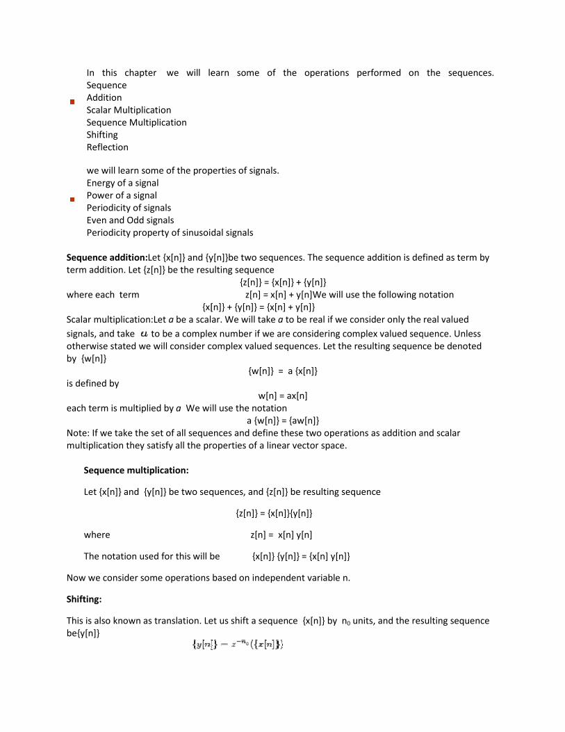
In this chapter we will learn some of the operations performed on the sequences.

Sequence

Addition

Scalar Multiplication

Sequence Multiplication

Shifting

Reflection

we will learn some of the properties of signals.

Energy of a signal

Power of a signal

Periodicity of signals

Even and Odd signals

Periodicity property of sinusoidal signals

Sequence addition:Let {x[n]} and {y[n]}be two sequences. The sequence addition is defined as term by

term addition. Let {z[n]} be the resulting sequence

where each term

{x[n]} + {y[n]} = {x[n] + y[n]}

Scalar multiplication:Let a be a scalar. We will take

signals, and take to be a complex number if

otherwise stated we will consider complex valued sequences. Let the resulting sequence be denoted

by {w[n]}

is defined by

each term is multiplied by a We will use the notation

Note: If we take the set of all sequences and define these two operations as addition and scalar

multiplication they satisfy all the properties of a linear

Sequence multiplication:

Let {x[n]} and {y[n]} be two sequences, and {z[n]} be resulting sequence

where

The notation used for this will be

Now we consider some operations based on independent variable

Shifting:

This is also known as translation. Let us shift a sequence

be{y[n]}

we will learn some of the operations performed on the sequences.

will learn some of the properties of signals.

Periodicity property of sinusoidal signals

{x[n]} and {y[n]}be two sequences. The sequence addition is defined as term by

term addition. Let {z[n]} be the resulting sequence

{z[n]} = {x[n]} + {y[n]}

z[n] = x[n] + y[n]We will use the following notation

{x[n]} + {y[n]} = {x[n] + y[n]}

be a scalar. We will take a to be real if we consider only the real valued

to be a complex number if we are considering complex valued sequence. Unless


{w[n]} = a {x[n]}

w[n] = ax[n]

We will use the notation

a {w[n]} = {aw[n]}


multiplication they satisfy all the properties of a linear vector space.

{y[n]} be two sequences, and {z[n]} be resulting sequence

{z[n]} = {x[n]}{y[n]}

z[n] = x[n] y[n]

The notation used for this will be {x[n]} {y[n]} = {x[n] y[n]}

Now we consider some operations based on independent variable n.

known as translation. Let us shift a sequence {x[n]} by n0 units, and the resulting sequence

we will learn some of the operations performed on the sequences.

{x[n]} and {y[n]}be two sequences. The sequence addition is defined as term by

lowing notation

to be real if we consider only the real valued

we are considering complex valued sequence. Unless



units, and the resulting sequence

where is the operation of shifting the sequence right by n

x[n - n0]. We will use short notation

Figure below show some examples of shifting.

{x[n]}

{x[n-2]}

{x [n+1]}

Reflection:

Let {x[n]} be the original sequence, and {y[n]} be reflected sequence, then y[n] is defined by

{x[n]}

is the operation of shifting the sequence right by n0 unit. The terms are defined

]. We will use short notation {x[n - n0]} to denote shift by n0.

Figure below show some examples of shifting.

Consider the figure to the left.

A negative value of n0 means shift

A positive value of n0 means shift towards left.


y[n] = x[-n]

unit. The terms are defined by y[n] =

means shift towards right.

means shift towards left.


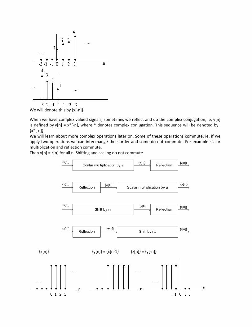
We will denote this by {x[-n]}

When we have complex valued signals, sometimes we reflect and do the complex conjugation, ie, y[n]

is defined by y[n] = x*[-n], where * denotes complex conjugation. This sequence will be denoted by

{x*[-n]}.

We will learn about more complex operations later on. Some of these operations commute, ie. if we

apply two operations we can interchange their order and some do not commute. For example scalar

multiplication and reflection commute.

Then v[n] = z[n] for all n. Shifting and scaling do not commute.

{x[n]} {y[n]} = {x[n-1} {z[n]} = {y[-n]}

{x[n]} {w[n]} = {x[

We can combine many of these operations in one step, for example {y[n]} may be defined as

[3-n].

Some Properties of signals

Energy of a Signal:

The total energy of a signal {x[n]} is defined by

A signal is referred to as an energy signal, if and only if the total energy of the signal E

Power of a signal:If {x[n]} is a signal whose energy is not finite, we define power of the signal as

A signal is referred to as a power signal if the power P

An energy signal has a zero power and a power signal has infinite energy. There are signals which are

neither energy signals nor power signals. For example {x[n]} defined by

power or energy.

Periodic Signals:

An important class of signals that we encounter frequently is the class of periodic signals. We say that

a signal {x[n] is periodic with period N, where N is a positive integer, if the signal is unchanged by the

time shift of N ie.,

or x[n] = x[ n + N ] for all n.

Since {x[n]} is same as {x[n+N]} , it is also periodic so we get

{x[n]} = {x[n+N]} = {x[n+N+N]}

Generalizing this we get {x[n]} = {x[n+kN]}, where k is a positive integer. From

periodic with 2N, 3N,... The fundamental period N

is periodic.

{w[n]} = {x[-n]} {u[n]} = {w[n-1]}

We can combine many of these operations in one step, for example {y[n]} may be defined as

The total energy of a signal {x[n]} is defined by

to as an energy signal, if and only if the total energy of the signal Ex

If {x[n]} is a signal whose energy is not finite, we define power of the signal as

A signal is referred to as a power signal if the power Px satisfies the condition


neither energy signals nor power signals. For example {x[n]} defined by x[n] = n does not have finite



{x[n]} = {x[n + N]}

, it is also periodic so we get

{x[n]} = {x[n+N]} = {x[n+N+N]} = {x[n+2N]}

Generalizing this we get {x[n]} = {x[n+kN]}, where k is a positive integer. From this we see that

periodic with 2N, 3N,... The fundamental period N0 is the smallest positive value N for which the signal

We can combine many of these operations in one step, for example {y[n]} may be defined as y[n] = 2x

x is finite.

If {x[n]} is a signal whose energy is not finite, we define power of the signal as


does not have finite



this we see that {x[n]} is

is the smallest positive value N for which the signal

The signal illustrated below is periodic with fundamental period N

By change of variable we can write

we see that

for all integer values of k positive, negative or zero. By definition, period of a signal is always a positive

integer N.

Except for a all zero signal all periodic signals have infinite energy. They may have finite power. Let

{x[n]} be periodic with period N, then the power P

where k is largest integer such that

be same for all terms. We see that k is approximately equal to

large M we get 2M/N terms and limit

Even and odd signals:

A real valued signal {x[n]} is referred to as an even signal if it is identical to its time reversed

counterpart ie, if

{x[n]} = {x[-n]}

A real signal is referred to as an odd signal if

An odd signal has value 0 at n = 0 as

Given any real valued signal {x[n]} we can write it as a sum of an even signal and an odd signal.

The signal illustrated below is periodic with fundamental period N0 = 4

By change of variable we can write {x[n]} = {x[n+N]} as {x[m-N]} = {x[m]} and then arguing as before,

{x[n]} = {x[n+kN]},



{x[n]} be periodic with period N, then the power Px is given by

is largest integer such that kN -1 ≤ M. Since the signal is periodic, sum over one period will

be same for all terms. We see that k is approximately equal to M/N (it is integer part of this) and for

terms and limit 2M/(2M +1) as M goes to infinite is one we get

is referred to as an even signal if it is identical to its time reversed

is referred to as an odd signal if

{x[n]} = {-x[-n]}

An odd signal has value 0 at n = 0 as x[0] = -x[n] = - x[0]

{x[n]} we can write it as a sum of an even signal and an odd signal.

N]} = {x[m]} and then arguing as before,



≤ M. Since the signal is periodic, sum over one period will

M/N (it is integer part of this) and for

as M goes to infinite is one we get

is referred to as an even signal if it is identical to its time reversed

{x[n]} we can write it as a sum of an even signal and an odd signal.

Consider the signals

Ev ({x[n]}) = {xe[n]} = {1/2 (x[n] + x[

and Od ({x[n]}) = {xo[n]} = {1/2(x[n]

We can see easily that

{x[n]} = {xe[n]} + {xo

The signal {xe[n]} is called the even part of

signal. Similarly, {xo[n]} is called the odd part of {x[n]} and is an odd signal. When we have complex

valued signals we use a slightly different terminology. A complex valued signal {x[n]} is refer

a conjugate symmetric signal if

{x[n]} = {x*[-n]}

where x* refers to the complex conjugate of x. Here we do reflection and complex conjugation. If

{x[n]} is real valued this is same as an even signal.

A complex signal {x[n]} is referred to as a conjugate antisymmetric signal if

We can express any complex valued signal as sum conjugate symmetric and conjugate antisymmetric

signals. We use notation similar to above

Ev({x[n]}) = {xe[n]} = {1/2(x[n] + x*[

and Od ({[n]}) = {xo[n]} = {1/2(x[n]

then {x[n]} = {xe[n]} + {xo[n]}

We can see easily that {xe[n]} is conjugate symmetric signal and

signal. These definitions reduce to even and odd signals in case signals takes only real values.

Periodicity properties of sinusoidal signals:

Let us consider the signal. We see that if we replace

the signal with frequency

continuous time signal

time we need to consider frequency interval of length 2π only. As we increase

oscillates more and more rapidly. But if we further increase frequency from π to 2π the rate of

oscillations decreases. This can be seen easily by plotting signal

The signal is not periodic for every value of. For the signal to be periodic with period N

we should have

that is should be some multiple of 2π.

or

Thus signal is periodic if and only if

Above observations also hold for complex exponential signal

Discrete-Time Systems:

Consider the signals

[n]} = {1/2 (x[n] + x[-n])}

[n]} = {1/2(x[n] -x [-n])}

o[n]}

[n]} is called the even part of {x[n]}. We can verify very easily that {xe

[n]} is called the odd part of {x[n]} and is an odd signal. When we have complex

valued signals we use a slightly different terminology. A complex valued signal {x[n]} is refer



signal {x[n]} is referred to as a conjugate antisymmetric signal if

{x[n]} = {-x*[-n]}


signals. We use notation similar to above

[n]} = {1/2(x[n] + x*[-n])}

[n]} = {1/2(x[n] - x*[-n])}

[n]} is conjugate symmetric signal and {xo[n]} is conjugate antisymmetric


Periodicity properties of sinusoidal signals:

Let us consider the signal. We see that if we replace by we get the same signal. In fact

and so on. This situation is quite different from

where each frequency is different. Thus in discrete

time we need to consider frequency interval of length 2π only. As we increase

apidly. But if we further increase frequency from π to 2π the rate of

oscillations decreases. This can be seen easily by plotting signal for several values of.

is not periodic for every value of. For the signal to be periodic with period N

should be some multiple of 2π.

is periodic if and only if is a rational number.

Above observations also hold for complex exponential signal

e[n]} is an even

[n]} is called the odd part of {x[n]} and is an odd signal. When we have complex

valued signals we use a slightly different terminology. A complex valued signal {x[n]} is referred to as




[n]} is conjugate antisymmetric


we get the same signal. In fact

and so on. This situation is quite different from

where each frequency is different. Thus in discrete

to π signal

apidly. But if we further increase frequency from π to 2π the rate of

for several values of.

is not periodic for every value of. For the signal to be periodic with period N > 0,

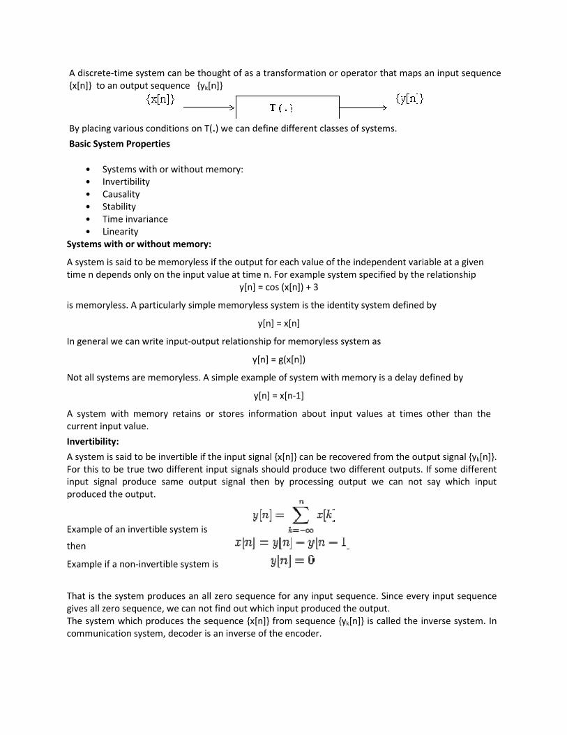
A discrete-time system can be thought of as a transformation or operator that maps an input sequence

{x[n]} to an output sequence {yk[n]}

By placing various conditions on T(

Basic System Properties

• Systems with or without memory:

• Invertibility

• Causality

• Stability

• Time invariance

• Linearity

Systems with or without memory:

A system is said to be memoryless if the output for each value of the independent variable at a given

time n depends only on the input value at time n. For example system specified by the relationship

is memoryless. A particularly simple memoryless

In general we can write input-output relationship for memoryless system as

Not all systems are memoryless. A simple example of system with memory is a delay defined by

A system with memory retains or stores information about input values at times other than the

current input value.

Invertibility:

A system is said to be invertible if the input signal {x[n]} can be recovered from the output signal {y

For this to be true two different input signals should produce two different outputs. If some different

input signal produce same output signal then by processing output we can not say which input

produced the output.

Example of an invertible system is

then

Example if a non-invertible system is

That is the system produces an all zero sequence for any input sequence. Since every input seque

gives all zero sequence, we can not find out which input produced the output.

The system which produces the sequence {x[n]} from sequence {y

communication system, decoder is an inverse of the encoder.

time system can be thought of as a transformation or operator that maps an input sequence

[n]}

By placing various conditions on T(.) we can define different classes of systems.

Systems with or without memory:

if the output for each value of the independent variable at a given


y[n] = cos (x[n]) + 3

is memoryless. A particularly simple memoryless system is the identity system defined by

y[n] = x[n]

output relationship for memoryless system as

y[n] = g(x[n])


y[n] = x[n-1]


A system is said to be invertible if the input signal {x[n]} can be recovered from the output signal {y



invertible system is

That is the system produces an all zero sequence for any input sequence. Since every input seque

gives all zero sequence, we can not find out which input produced the output.

The system which produces the sequence {x[n]} from sequence {yk[n]} is called the inverse system. In

communication system, decoder is an inverse of the encoder.

time system can be thought of as a transformation or operator that maps an input sequence

if the output for each value of the independent variable at a given


system is the identity system defined by



A system is said to be invertible if the input signal {x[n]} can be recovered from the output signal {yk[n]}.



That is the system produces an all zero sequence for any input sequence. Since every input sequence

[n]} is called the inverse system. In

Causality :

A system is causal if the output at anytime depends only on values of the input at the present time

and in the past.

All memoryless systems are causal. An accumulator system defined by

is also causal. The system defined by

is noncausal.

For real time system where n actually denoted time causality is mportant. Causality is not an

essential constraint in applications where n is not time, for example, image processing. If we are

doing processing on recorded data, then also causality may not be required.

Stability :

There are several definitions for stability. Here we will consider bounded input bonded output (BIBO)

stability. A system is said to be BIBO stable if every bounded input

say that a signal {x[n]} is bounded if

The moving average system

is stable as y[n] is sum of finite numbers and so it is bounded. The accumulator system defined by

is unstable. If we take {x[n]} = {u[n]}, the unit step then y[0] = 1, y[1] = 2, y[2] = 3,

≥ 0 so y[n]grows without bound.

Time invariance :

A system is said to be time invariant if the behavior and characteristics of the system do not change

with time.Thus a system is said to be time invariant if a time delay or time advance in the input signal

leads to identical delay or advance in the output signal. Mathematically if

then

Let us consider the accumulator system

If the input is now {x1[n]} = {x[n-n0]}


y[n] = f(x[n], x[n-1],...)

All memoryless systems are causal. An accumulator system defined by

also causal. The system defined by



ocessing on recorded data, then also causality may not be required.


stability. A system is said to be BIBO stable if every bounded input produces a bounded output. We

say that a signal {x[n]} is bounded if

|x[n]| < M < ∞ for all n


{x[n]} = {u[n]}, the unit step then y[0] = 1, y[1] = 2, y[2] = 3, are y[n] = n +1, n


time.Thus a system is said to be time invariant if a time delay or time advance in the input signal

leads to identical delay or advance in the output signal. Mathematically if

{y[n]} = T ({x[n]})

{y[n-n0]} = T({x[n-n0]}) for any n0

Let us consider the accumulator system

]} then the corresponding output is





produces a bounded output. We


are y[n] = n +1, n


time.Thus a system is said to be time invariant if a time delay or time advance in the input signal

The shifted output signal is given by

The two expression look different, but

by l = k - n0 in the first sum then we see that

Hence, {y[n]} = {y[n-n0]} and the system is time

defined by y[n] = nx[n]

if

while

and so the system is not time-invariant. It is time varying. We can also see this by giving a counter

example. Suppose input is

then output is which is definitely not a shifted version version of all zero sequence.

Linearity :

This is an important property of the system. We will see later that if we have system which is linear

and time invariant then it has a very co

important property of superposition: if an input consists of weighted sum of several signals, the nthe

output is also weighted sum of the responses of the system to each of those input signals.

Mathematically let be the response of the system to the input

response of the system to the input. Then the system is linear if:

Additivity: The response to

Homogeneity: The response to

considering only real signals and

signals.

Continuity: Let us consider

that

Let the corresponding output signals be denoted by

We say that system posseses the continuity property if the response of the system to the limiting

input is limit of the responses.

The additivity and continuity properties can be replaced by requiring that system is additive for

countably infinite number of signals i.e. response to

The shifted output signal is given by

The two expression look different, but infact they are equal. Let us change the index of summation

in the first sum then we see that

]} and the system is time-invariant. As a second example consider the system

invariant. It is time varying. We can also see this by giving a counter

then output is all zero sequence. If the input is

which is definitely not a shifted version version of all zero sequence.


and time invariant then it has a very compact representation. A linear system possesses the



be the response of the system to the input and let

response of the system to the input. Then the system is linear if:

is

is , where is any real number if we are

is any complex number if we are considering complex valued

be countably infinite number of signals such

Let the corresponding output signals be denoted by and


is limit of the responses.


mber of signals i.e. response to

infact they are equal. Let us change the index of summation

invariant. As a second example consider the system

invariant. It is time varying. We can also see this by giving a counter

input is

which is definitely not a shifted version version of all zero sequence.


mpact representation. A linear system possesses the



and let be the

is any real number if we are

is any complex number if we are considering complex valued

be countably infinite number of signals such



Most of the books do not mention the continuity property. They state only finite additivity and

homogeneity. But from finite additivity we can not deduce countable additivity. This distinction

becomes very important in continuous time systems.

A system can be linear without being time invariant and it can be time invariant without being linear.

If a system is linear, an all zero input sequence will produce a all zero output sequence. Let

denote the all zero sequence, then. If

or,

Consider the system defined by

This system is not linear. This can be verified in several ways. If the input is all zero sequence

output is not an all zero sequence. Alth

system is nonlinear. The output of this system can be represented as sum of a linear system and

another signal equal to the zero input response. In this case the linear system is

and the zero-input response is

Such systems correspond to the class of incrementally linear system. System is linear in term of

differnce signal i.e if we define

and the system is linear.

The Convolution Sum:

The representation of discrete time signals in terms of impulses.

The key idea is to express an arbitrary discrete time signal as weighted sum of time shifted impulses.

Consider the product of signal

and

Using these relations we can write

A graphical illustration is shown below

is



very important in continuous time systems.



all zero sequence, then. If then by homogeneity property

This system is not linear. This can be verified in several ways. If the input is all zero sequence

output is not an all zero sequence. Although the defining equation is a linear equation is x and y the


another signal equal to the zero input response. In this case the linear system is

for all n


differnce signal i.e if we define and. Then in terms of

The representation of discrete time signals in terms of impulses.


and the impulse sequence. We know that

A graphical illustration is shown below





then by homogeneity property

This system is not linear. This can be verified in several ways. If the input is all zero sequence , the

ough the defining equation is a linear equation is x and y the



and. Then in terms of


(4.1)

Fig 4.1

Given an arbitrary sequence we can write it as a linear combination of shifted unit

impulses , where the weights of their combination are x[k], the kth

term of the sequence.

For any given n, in the summation

there is only one term which is non-zero and so we do not have to worry about the convergence.

Consider the unit step sequence {u[n]}. Since , and , it has

representation

The Discrete Time Impulse response of linear Time Invariant System:

We use linearity property of the system to represent its response in terms of its response shifted

impulse sequences. The time invariance further simplifies their representation. Let be the

input signal and be the output sequence, and T( ) represent the linear system

using (4.1)

Now we use the linearity property of the system we get

Note that without countable additivity property the last step is not justified (From finite additivity we

can not get countable additivity). Let us define

i.e. is the response of the system to a delayed unit sample sequence. Then we see

The output signal is linear combination of the signals.

In general the responses need not be related to each other for different values of k.

However, if linear system is also time-invariant, then these responses are related. Let us define

impulse response (unit sample response)

Then

For the LTI system output {y[n]} is given by

(4.2)

This result is know as convolution of sequences and. Thus output signal for an LTI system is

convolution of input signal and the impulse response. This operation is symbolically

represented by

(4.3)

We see that equation (4.2) expresses the response of an LTI system to an arbitrary signal in terms of

the systems response to unit impulse. Thus an LTI system is completely specified by its impulse

response.

The nth

term in the equation (4.2) is given by

(4.4)

This is known as convolution sum. To convolve two sequences, we have to calculate this convolution

sum for all values of n. Since right hand side is sum of infinite series, we assume that this sum is well

defined.

Example:

Consider and shown below

Fig 4.2

Since only and one non zero we have

These one illustrated below

Fig 4.3

Here we have done calculation according to equation (4.2).

To do calculation according to equation (4.4) we first plot - as function of k and

as function of k for some fixed values of n. Then multiply sequence and term by

term to obtain sequence. Than final the sum of the terms of the sequence. This is illustrated below

Fig 4.4

One can see easily that for other value of n is all zero sequence and for these value

of n, output is zero.

Properties of discrete-time linear convolution and system properties

If and are sequences, then the following useful properties of the discrete

time convolution can be shown to be true

1. Commutativity

2. Associativity

`

3. Distributivity over sequence addition

4. The identity sequence

5. Delay operation

6. Multiplication by a constant

Note that these properties are true only if the convolution sum (4.4) exists for every n.

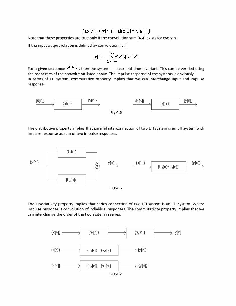
If the input output relation is defined by convolution i.e. if

For a given sequence , then the system is linear and time invariant. This can be verified using

the properties of the convolution listed above. The impulse response of the systems is obviously.

In terms of LTI system, commutative property implies that we can interchange input and impulse

response.

Fig 4.5

The distributive property implies that parallel interconnection of two LTI system is an LTI system with

impulse response as sum of two impulse responses.

Fig 4.6

The associativity property implies that series connection of two LTI system is an LTI system. Where

impulse response is convolution of individual responses. The commutativity property implies that we

can interchange the order of the two system in series.

Fig 4.7

Since an LTI system is completely characterized by its impulse response, we can specify system-

properties in terms of impulse response.

1. Memoryless system: From equation (4.4) we see that an LTI system is memory less if and only

if.

2. Causality for LTI system: The output of a causal system depends only on preset and past-

values of the input. In order for a system to be causal must not depend on for.

From equation (4.4) we see that for this to be true, all of the terms that multiply

values of for must be zero.

put to get

or

Thus impulse response for a causal LTI system must satisfy the condition h[n] = 0 for n

< 0.

If the impulse response satisfies this condition, the system is causal. For a causal system we

can write

or

We say a sequence is causal if , for n < 0.

3. Stability for LTI system: A system is stable if every bounded input produces a bonded output.

Consider input such that for all n.

Taking absolute value

From triangle inequality for complex numbers we get

Using property that

Since each we get

If the impulse response is absolutely summable, that is

(4.5)

then

and is bounded for all n, and hence system is stable. Therefore equation (4.5) is sufficient

condition for system to be stable. This condition is also necessary. This is prove by showing that if

condition (4.5) is violated then we can find a bounded input which produces an unbounded output.

Let

Let

This is a bounded sequence

So y[0] is unbounded. Thus, the stability of a discrete time linear time invariant system is equivalent to

absolute summability of the impulse response.

Causal LTI systems described by difference equations

An important subclass of linear time invariant system is one where the input and output sequences

satisfy constant coefficient linear difference equation

(4.6)

The constants, is input sequence and is output sequence. We can solve equation

(4.6) in a manner analogous to the differential equation solution, but for discrete time we can use a

different approach. Assume that. We can write

(4.7)

In order to find we need previous N values of the output. Thus if we know the input

sequence and a set of initial condition we can find values of.

Example: Consider the difference equation

then

Let us take

This system is not linear for all values of the initial condition. For a linear system all zero input

sequence must produce a all zero output sequence. But if C is different from zero, then output

sequence is not an all system is linear. System is not time invariant in general. Suppose input

is than we have

If we use input as then

It is obvious that second sequence is not a shifted version of the first sequence unless. The system is

linear time invariant if we assume initial rest condition, i.e. if then. With initial rest

condition the system described by constant coefficient-linear difference equation is linear, time

invariant and causal.

The equation of the form (4.7) is called recursive equation if , since it specifies a recursive

algorithm for finding out the output sequence. In special case

Here is completely specified in terms of the input. Thus this equation is called non

equation. If input , then we see that the output is equal to impulse response

The impulse response is non-zero for finitely many values. A system with the property that impulse

response is non-zero only for finitely many values is known as finite impulse response (FIR) system. A

system described by non-recursive equation is always F

generally has a response which is non

infinite impulse response system (IIR). A system described by recessive equation may have a finite

impulse response.

The Discrete Time Fourier Transform

In the previous chapter we used the time domain representation of the signal. Given any signal {x[n]}

we can write it as linear combination of basic signals.

been found very useful is frequency domain representation. In the mid 1960s an algorithm for

calculation of the Fourier transform was discovered, known as the Fast

algorithm. This spurred the development of digital signal processing in many areas.

The Fourier representation of signals derives its importance from the fact that exponential signals

are eigenfunctions for the discrete time LTI systems. What we mean by this is that if

signal to an LTI system then output is given by. Let us co

Then the output is given by

=

=

=

=

where assuming that the summation in right

output is same exponential sequence multiplied by a constant that depends

algorithm for finding out the output sequence. In special case , we have

is completely specified in terms of the input. Thus this equation is called non

, then we see that the output is equal to impulse response

zero for finitely many values. A system with the property that impulse

zero only for finitely many values is known as finite impulse response (FIR) system. A

recursive equation is always FIR. A system described recursive equation

generally has a response which is non-zero for infinite duration and such systems one known as


The Discrete Time Fourier Transform


we can write it as linear combination of basic signals. Another representation of signals that has

useful is frequency domain representation. In the mid 1960s an algorithm for

calculation of the Fourier transform was discovered, known as the Fast-Fourier Transform (FFT)



are eigenfunctions for the discrete time LTI systems. What we mean by this is that if

signal to an LTI system then output is given by. Let us consider an LTI system with impulse response.

assuming that the summation in right-hand side converges. Thus

output is same exponential sequence multiplied by a constant that depends on the value of.

Fig 5.1

(4.8)

is completely specified in terms of the input. Thus this equation is called non-recursive

, then we see that the output is equal to impulse response

zero for finitely many values. A system with the property that impulse

zero only for finitely many values is known as finite impulse response (FIR) system. A

IR. A system described recursive equation

zero for infinite duration and such systems one known as



Another representation of signals that has

useful is frequency domain representation. In the mid 1960s an algorithm for

Fourier Transform (FFT)



are eigenfunctions for the discrete time LTI systems. What we mean by this is that if is input

nsider an LTI system with impulse response.

hand side converges. Thus

on the value of.

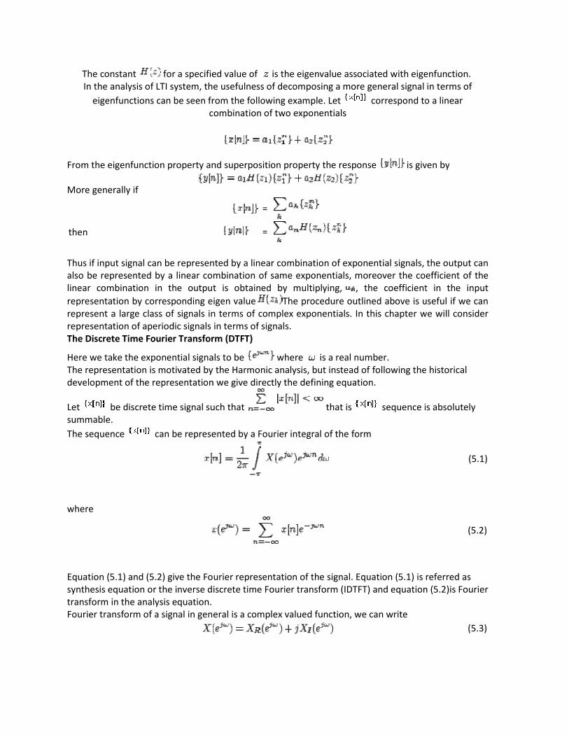
The constant for a specified value of

In the analysis of LTI system, the usefulness of decomposing a more general signal in terms of

eigenfunctions can be seen from the following example. Let

combination of two exponentials

From the eigenfunction property and superposition property the response

More generally if

then

Thus if input signal can be represented by a linear combination of exponential signals, the output can

also be represented by a linear combination of same exponentials, moreover the

linear combination in the output is obtained by multiplying,

representation by corresponding eigen value

represent a large class of signals in terms of comp

representation of aperiodic signals in terms of signals.

The Discrete Time Fourier Transform (DTFT)

Here we take the exponential signals to be

The representation is motivated by the Harmonic analysis, but instead of following the historical

development of the representation we give directly the defining equation.

Let be discrete time signal such that

summable.

The sequence can be represented by a Fourier integral of the form

where

Equation (5.1) and (5.2) give the Fourier representation of the signal. Equation (5.1) is referred as

synthesis equation or the inverse discrete time Fourier transform (IDTFT) and

transform in the analysis equation.

Fourier transform of a signal in general is a complex valued function, we can write

for a specified value of is the eigenvalue associated with eigenfunction.


can be seen from the following example. Let correspond to a linear

combination of two exponentials

From the eigenfunction property and superposition property the response is given by

=

=


also be represented by a linear combination of same exponentials, moreover the coefficient of the

linear combination in the output is obtained by multiplying, , the coefficient in the input

representation by corresponding eigen value The procedure outlined above is useful if we can

represent a large class of signals in terms of complex exponentials. In this chapter we will consider

representation of aperiodic signals in terms of signals.

The Discrete Time Fourier Transform (DTFT)

Here we take the exponential signals to be where is a real number.

motivated by the Harmonic analysis, but instead of following the historical

development of the representation we give directly the defining equation.

be discrete time signal such that that is sequence is absolutely

be represented by a Fourier integral of the form


synthesis equation or the inverse discrete time Fourier transform (IDTFT) and equation (5.2)is Fourier

Fourier transform of a signal in general is a complex valued function, we can write

is the eigenvalue associated with eigenfunction.


correspond to a linear

is given by


coefficient of the

, the coefficient in the input

The procedure outlined above is useful if we can

lex exponentials. In this chapter we will consider

motivated by the Harmonic analysis, but instead of following the historical

sequence is absolutely

(5.1)

(5.2)


equation (5.2)is Fourier

(5.3)

where is the real part of

use a polar form

where is magnitude and

simply, the spectrum to refer to. Thus

called the phase spectrum.

From equation (5.2) we can see that

interpret (5.1) as Fourier coefficients in the representation of a perotic function. In the Fourier series

analysis our attention is on the periodic function, here we are concerned with the representation of

the signal. So the roles of the two equation are interchanged compared to the Fourier series analysis

of periodic signals.

Now we show that if we put equation (5.2) in equation (5.1) we indeed get the signal.

Let

where we have substituted

Since we have used n as index on the left hand side we have used m as the index variable for the sum

defining the Fourier transform. Under our assumption that

we can interchange the order of integration and summation. Thus

The integral with the parentheses can be evaluated as

if then

and

if then

=

=

= 0

Thus in equation (5.5) there is only one non

and is imaginary part of the function. We can also

is the phase of. We also use the term Fourier spectrum or

simply, the spectrum to refer to. Thus is called the magnitude spectrum and

From equation (5.2) we can see that is a periodic function with period i.e.. We can



signal. So the roles of the two equation are interchanged compared to the Fourier series analysis

Now we show that if we put equation (5.2) in equation (5.1) we indeed get the signal.

from (5.2) into equation (5.1) and called the result as.


defining the Fourier transform. Under our assumption that sequence is absolutely summable

he order of integration and summation. Thus

The integral with the parentheses can be evaluated as

Thus in equation (5.5) there is only one non-zero term in RHS, corresponding to

is imaginary part of the function. We can also

(5.4)

is the phase of. We also use the term Fourier spectrum or

is

i.e.. We can



signal. So the roles of the two equation are interchanged compared to the Fourier series analysis

equation (5.1) and called the result as.


sequence is absolutely summable

(5.5)

, and we

get. This result is true for all values of n and so equation (5.1) is indeed a representation of

signal in terms eigenfunctions

In above demonstration we have as

of signals which can be represented by equation (5.1) is equivalent to considering the convergence of

the infinite sum in equation (5.2). If we fix a value of

complex valued series, whose partial sum is given by

The limit as if the partial sum

Since the limit

exists for every. Furthermore it can be shown that the series converges uniformly to a continuous

function of.

If a sequence has only finitely many non

transform exists. Since a stable sequence is by defin

Fourier transform also exits.

Example: Let

Fourier transform of this sequence will exist if it is absolutely summable. We have

This is a geometric series and sum exists if

Thus the Fourier transform of the sequence


in terms eigenfunctions

In above demonstration we have assumed that is absolutely summable. Determining the class


the infinite sum in equation (5.2). If we fix a value of then, RHS of equation (5.2) is a

plex valued series, whose partial sum is given by

if the partial sum exists if the series is absolutely summable.

by triangle inequality

exists by our assumption the limit

every. Furthermore it can be shown that the series converges uniformly to a continuous

If a sequence has only finitely many non-zero terms then it is absolutely summable and so the Fourier

transform exists. Since a stable sequence is by definition, an absolutely summable sequence, its

Fourier transform of this sequence will exist if it is absolutely summable. We have

This is a geometric series and sum exists if , in that case

transform of the sequence exists if. The Fourier transform is


is absolutely summable. Determining the class


then, RHS of equation (5.2) is a

exists if the series is absolutely summable.

every. Furthermore it can be shown that the series converges uniformly to a continuous

zero terms then it is absolutely summable and so the Fourier

ition, an absolutely summable sequence, its

exists if. The Fourier transform is

Where the last equality follows from sum of a geometric series, which exists if

Absolute summability is a sufficient condition for the existence of a Fourier transform. Fourier

transform also exists for square summable sequence.

For such signals the convergence is not uniform. This has implications in the design of discrete

system for filtering.

We also deal with signals that are neither so absolutely summable nor square summable. To deal

with some of these signals we allow impulse functions, which i

generalized function as a Fourier transform. The impulse function is defined by the following

properties

(a)

(b)

convolution property)

(c) if

Since is a periodic function,

If we substitute this in equation (5.1) we get

equality follows from sum of a geometric series, which exists if


transform also exists for square summable sequence.

convergence is not uniform. This has implications in the design of discrete


with some of these signals we allow impulse functions, which is not an ordinary function but a


if is continuous at ;(shifting or

if is continuous at

periodic function, let us consider

If we substitute this in equation (5.1) we get

(5.6)

i.e..


convergence is not uniform. This has implications in the design of discrete


s not an ordinary function but a


;(shifting or

(5.7)

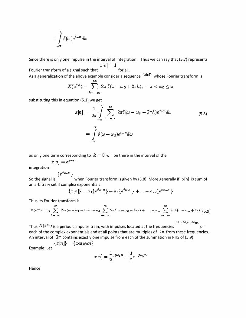
Since there is only one impulse in the interval of integration.

Fourier transform of a signal such that

As a generalization of the above example consider a sequence

substituting this in equation (5.1) we get

as only one term corresponding to

integration

So the signal is when Fourier transform is given by (5.8). More generally if

an arbitrary set if complex exponentials

Thus its Fourier transform is

Thus is a periodic impulse train, with impulses located at

each of the complex exponentials and at all points that are multiples of

An interval of contains exactly one impulse from each of the summation in RHS of (5.9)

Example: Let

Hence

Since there is only one impulse in the interval of integration. Thus we can say that (5.7) represents

that for all.

As a generalization of the above example consider a sequence whose Fourier transform is

substituting this in equation (5.1) we get

will be there in the interval of the

when Fourier transform is given by (5.8). More generally if x[n]

an arbitrary set if complex exponentials

is a periodic impulse train, with impulses located at the frequencies

each of the complex exponentials and at all points that are multiples of from these frequencies.

contains exactly one impulse from each of the summation in RHS of (5.9)

Thus we can say that (5.7) represents

whose Fourier transform is

(5.8)

x[n] is sum of

(5.9)

of

from these frequencies.

contains exactly one impulse from each of the summation in RHS of (5.9)

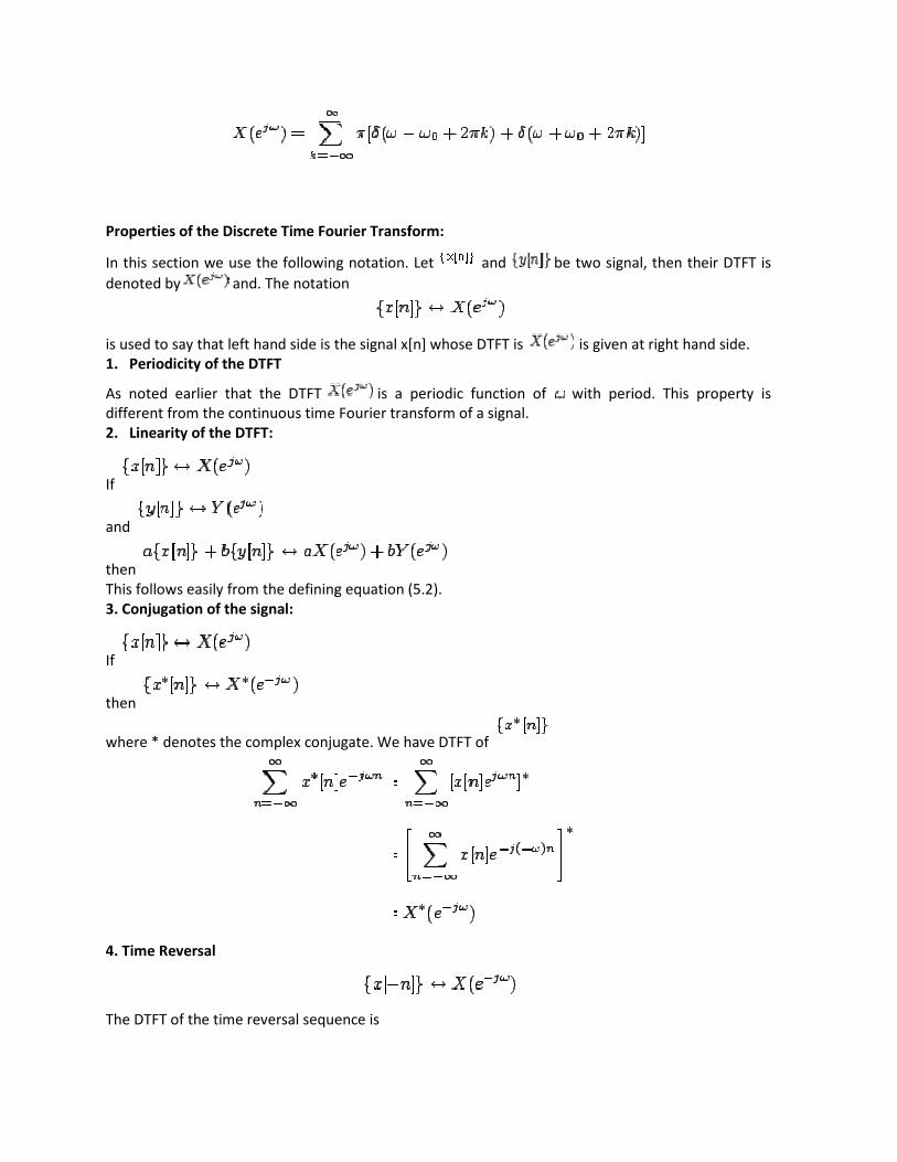
Properties of the Discrete Time Fourier Transform:

In this section we use the following notation. Let

denoted by and. The notation

is used to say that left hand side is the signal x[n] whose DTFT is

1. Periodicity of the DTFT

As noted earlier that the DTFT

different from the continuous time Fourier transform of a signal.

2. Linearity of the DTFT:

If

and

then

This follows easily from the defining equation (5.2).

3. Conjugation of the signal:

If

then

where * denotes the complex conjugate. We have DTFT of

4. Time Reversal

The DTFT of the time reversal sequence is

the Discrete Time Fourier Transform:

In this section we use the following notation. Let and be two signal, then their DTFT is

and. The notation

is used to say that left hand side is the signal x[n] whose DTFT is is given at right hand

is a periodic function of with period. This property is

different from the continuous time Fourier transform of a signal.

follows easily from the defining equation (5.2).

where * denotes the complex conjugate. We have DTFT of

The DTFT of the time reversal sequence is

be two signal, then their DTFT is

is given at right hand side.

with period. This property is

Let us change the index of summation as

5. Symmetry properties of the Fourier Transform:

If x[n] is real valued than

This follows from property 3. If x[n]

hence

expressing in real and imaginary parts we see that

which implies

and

That is real part of the Fourier transform is an even function of

function of.

The magnitude spectrum is given by

Hence magnitude spectrum of a real signal is an even function of.

The phase spectrum is given by

change the index of summation as

5. Symmetry properties of the Fourier Transform:

This follows from property 3. If x[n] is real valued then , so

in real and imaginary parts we see that

That is real part of the Fourier transform is an even function of and imaginary part is an odd

function of.

The magnitude spectrum is given by


and

and imaginary part is an odd

function of.


Thus the phase spectrum is an odd function of. We denote the symmetric and antisymmetric part of

a function by

Then using property (2) and (3) we see that

and using property (2) and (4) we can see that

6. Time shifting and frequency shifting:

These can be proved very easily by direct substitution of

and in equation (5.1).

7. Differencing and summation:

This follows directly from

Consider next the signal defined by

since , we are tempted to conclude that the DTFT of


Then using property (2) and (3) we see that

property (2) and (4) we can see that

Time shifting and frequency shifting:

These can be proved very easily by direct substitution of in equation(5.2)

in equation (5.1).

This follows directly from linearity property 2.

defined by

, we are tempted to conclude that the DTFT of is DTFT of


in equation(5.2)

linearity property 2.

is DTFT of

divided by. This is not entirely true as it ignores the possibility of a dc or average term that can result

from summation. The precise relationship is

We omit the proof of this property.

If we take then we get

8. Time and frequency scaling:

For continuous time signals we know that the Fourier transform of

define a signal we run into

integer say , then we get signal. This consists of taking

Thus the DTFT of this signal looks similar to the Fourier transform of a sampled signal. The result th

resembles the continuous time signal is obtained if we define a signal

For example


. The precise relationship is


then we get

For continuous time signals we know that the Fourier transform of is given by. However if we

we run into difficulty as the index must be an integer. Thus if

, then we get signal. This consists of taking sample of the original signal.

Thus the DTFT of this signal looks similar to the Fourier transform of a sampled signal. The result th

resembles the continuous time signal is obtained if we define a signal by

For example is illustrated below

Fig 5.2



is given by. However if we

must be an integer. Thus if is an

sample of the original signal.

Thus the DTFT of this signal looks similar to the Fourier transform of a sampled signal. The result that

The signal is obtained by inserting

Here we can note the time frequency uncertainly. Since

Fourier transform is compressed.

9. Diffentiation in frequency domain

Differentiating both sides with respect to

multiplying both sides by j we obtain

10. Passeval's relation:

We have

interchanging summation and integration we get

is obtained by inserting zeroes between successive value if signal.

the time frequency uncertainly. Since is expanded sequence, the

Diffentiation in frequency domain

Differentiating both sides with respect to , we obtain

multiplying both sides by j we obtain

interchanging summation and integration we get

zeroes between successive value if signal.

is expanded sequence, the

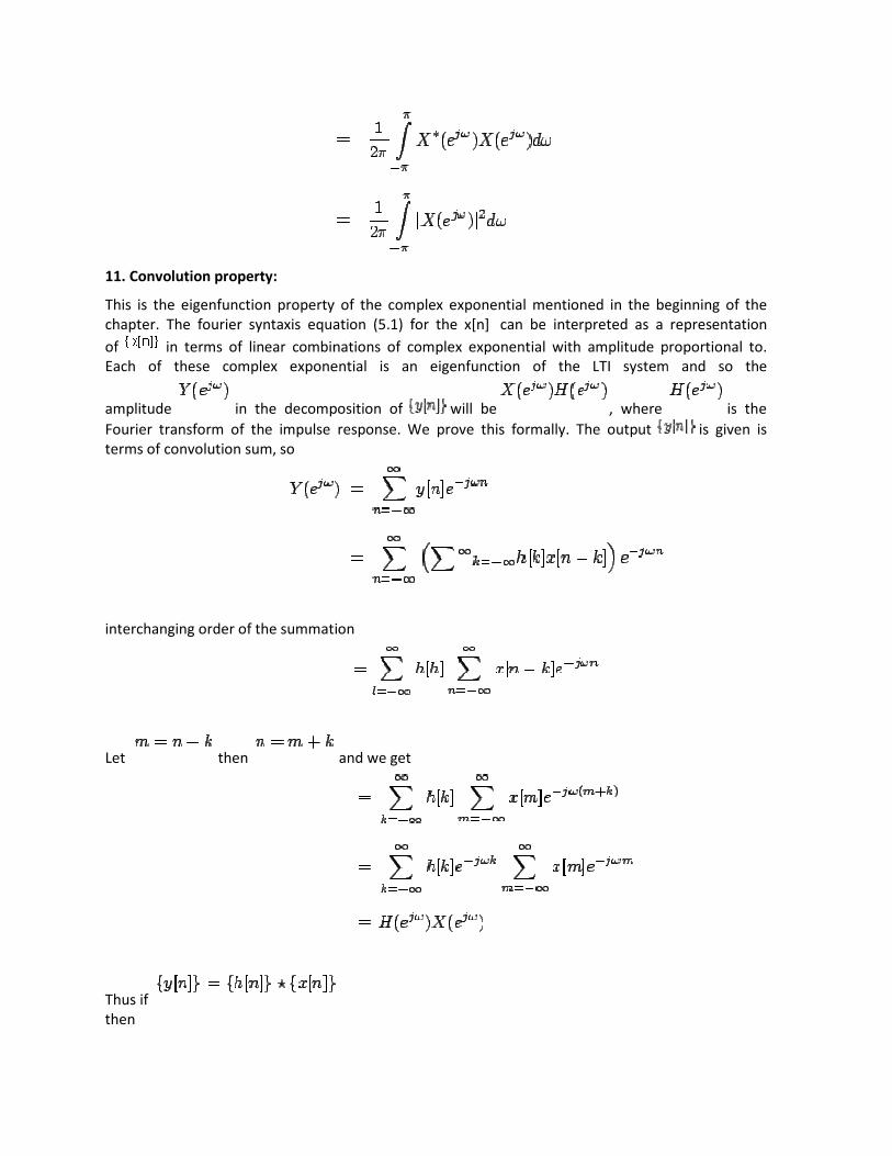
11. Convolution property:

This is the eigenfunction property of the complex exponential mentioned in the beginning of the

chapter. The fourier syntaxis equation (5.1) for the x[n]

of in terms of linear combinations of complex exponential with amplitude proportional to.

Each of these complex exponential is an eigenfunction of the LTI system and so the

amplitude in the decomposition of

Fourier transform of the impulse response. We prove this formally. The output

terms of convolution sum, so

interchanging order of the summation

Let then

Thus if

then


syntaxis equation (5.1) for the x[n] can be interpreted as a representation

in terms of linear combinations of complex exponential with amplitude proportional to.


in the decomposition of will be , where

Fourier transform of the impulse response. We prove this formally. The output

interchanging order of the summation

and we get


can be interpreted as a representation

in terms of linear combinations of complex exponential with amplitude proportional to.


is the

is given is

convolution in time domain becomes multiplication in the frequency domain. The fourier transform

of the impulse response is known as frequency response of the system.

12. The Modulation or windowing property

Let us find the DTFT of product of two sequences

Substituting for x[n] in terms of IDFT we get

interchanging order of integration and summation

This looks like convolution of two

and one periodic functions, and equation (5.21) is called periodic convolution. Thus

where denotes periodic convolution.

We summarize these properties in Table (5.1)

Table 5.1: Properties of Discrete time Fourier Transform

Aperiodic signal


is known as frequency response of the system.

Modulation or windowing property

Let us find the DTFT of product of two sequences

in terms of IDFT we get

interchanging order of integration and summation

This looks like convolution of two functions, only the interval of integration is

one periodic functions, and equation (5.21) is called periodic convolution. Thus

denotes periodic convolution.

We summarize these properties in Table (5.1)

Discrete time Fourier Transform

Discrete time fourier transform

(5.20)


to.

one periodic functions, and equation (5.21) is called periodic convolution. Thus

denotes periodic convolution.

The frequency response of systems characterized by linear constant coefficient difference

equation.

As we have seen earlier, constant coefficient linear difference equation with zero initial condition can

be used to describe some linear time invariant systems.

The input-output and

We assume that Fourier transforms of

response of the system) exist, then convolution property implies that


have seen earlier, constant coefficient linear difference equation with zero initial condition can

be used to describe some linear time invariant systems.

are related by

We assume that Fourier transforms of and , ( is the impulse

response of the system) exist, then convolution property implies that


have seen earlier, constant coefficient linear difference equation with zero initial condition can

(5.22)

is the impulse

Taking fourier transform of both sides of equation (5.22) and using linearity and time shifting

property of the Fourier transform we get

or

Thus we see that the frequency response is ratio of polynomials in the variable. The numerator

coefficients are the coefficients of

coefficients of in equation (5.22). Thus we can write the frequency resp

inspection.

Example 2: Consider an LTI system initially at rest described by the difference equation

The frequency response of the system is

We can use the inverse fourier transform to get the impulse response

Discrete Fourier series Representation of a periodic signal

Suppose that is a periodic signal with period N, that is

As is continues time periodic signal, we would like to represent

complex exponential signals are given by

All these signals have frequencies is that are multiples of the some fundamental frequency,


property of the Fourier transform we get

see that the frequency response is ratio of polynomials in the variable. The numerator

in equation (5.22) and denominator coefficients are the

in equation (5.22). Thus we can write the frequency resp

Consider an LTI system initially at rest described by the difference equation

The frequency response of the system is

We can use the inverse fourier transform to get the impulse response

Representation of a periodic signal

is a periodic signal with period N, that is

As is continues time periodic signal, we would like to represent in terms of discrete time

complex exponential signals are given by

All these signals have frequencies is that are multiples of the some fundamental frequency,


(5.23)

see that the frequency response is ratio of polynomials in the variable. The numerator

in equation (5.22) and denominator coefficients are the

in equation (5.22). Thus we can write the frequency response by

Consider an LTI system initially at rest described by the difference equation

in terms of discrete time

(6.1)

All these signals have frequencies is that are multiples of the some fundamental frequency, , and

thus harmonically related.

These are two important distinction between continuous time and discrete time complex exponential.

The first one is that harmonically related continuous time complex exponential are all

distinct for different values of k , while there are only N different signals in the set.

The reason for this is that discrete time complex exponentials which differ in frequency by integer

multiple of are identical. Thus

So if two values of k differ by multiple of N , they represent the same signal. Another difference

between continuous time and discrete time complex exponential is that for

different k have period which changes with k. In discrete time exponential, if k and N are

relative prime than the period is N and not N/k. Thus if N is a prime number, all the complex

exponentials given by (6.1) will have period N. In a manner analogous to the continuous time, we

represent the periodic signal as

(6.2)

where

(6.3)

In equation (6.2) and (6.3) we can sum over any consecutive N values. The equation (6.2) is synthesis

equation and equation (6.3) is analysis equation. Some people use the faction 1 /N in analysis

equation. From (6.3) we can see easily that

Thus discrete Fourier series coefficients are also periodic with the same period N.

Example 1:

So, and , since the signal is periodic with periodic with period 5, coefficients

are also periodic with period 5, and.

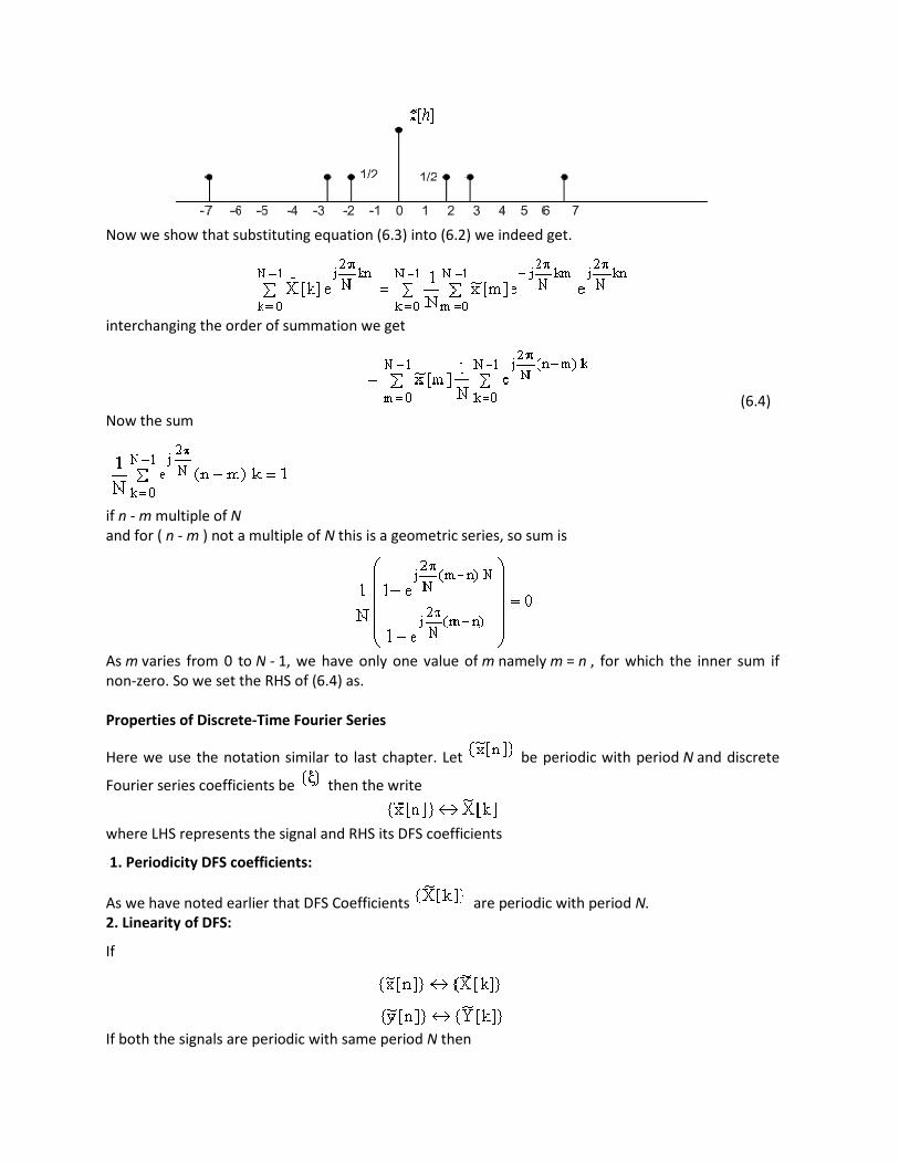
Now we show that substituting equation (6.3) into (6.2) we indeed get.

interchanging the order of summation we get

(6.4)

Now the sum

if n - m multiple of N

and for ( n - m ) not a multiple of N this is a geometric series, so sum is

As m varies from 0 to N - 1, we have only one value of m namely m = n , for which the inner sum if

non-zero. So we set the RHS of (6.4) as.

Properties of Discrete-Time Fourier Series

Here we use the notation similar to last chapter. Let be periodic with period N and discrete

Fourier series coefficients be then the write

where LHS represents the signal and RHS its DFS coefficients

1. Periodicity DFS coefficients:

As we have noted earlier that DFS Coefficients are periodic with period N.

2. Linearity of DFS:

If

If both the signals are periodic with same period N then

3. Shift of a sequence:

(6.5)

(6.6)

To prove the first equation we use equation (6.3). The DFS coefficients are given by

let n - m = l , we get

since is periodic we can use any N consecutive values, then

We can prove the relation (6.6) in a similar manner starting from equation (6.3)

4. Duality:

From equation (6.2) and (6.3) we can see that synthesis and analysis equation differ only in sign of the

exponential and factor 1/N. If is periodic with period N , then is also periodic with

period N. So we can find the discrete fourier series coefficients of sequence.

From equation (6.2) we see that

Thus

Interchanging the role of k and n we get

comparing this with (6.3) we see that DFS coefficients of are the original

periodic sequence is reversed in time and multiplied by N. This is known as duality property. If

(6.7)

then

(6.8)

5. Complex conjugation of the periodic sequence:

substituting in equation (6.3) we get

6. Time reversal:

From equation (6.3) we have the DFS coefficient

putting m = - n we get

Since is periodic, we can use any N consecutive values

7. Symmetry properties of DFS coefficient:

In the last chapter we discussed some symmetry properties of the discrete time Fourier transform of

aperiodic sequence. The same symmetry properties also hold for DFS coefficients and their derivation

is also similar in style using linearity, conjugation and time reversal properties DFS coefficients.

8. Time scaling:

Let us define

sequence is obtained by inserting ( m - 1) zeros between two consecutive values of. Thus

Thus is also periodic, but period is mN. The DFS coefficients are given by

putting

as non zero terms occur only when r = 0

If we define then is periodic with period equal to least common multiple (LCM)

of M and N. The relationship between DFS coefficients is not simple and we omit it here.

9. Difference

This follows from linearity property.

10. Accumulation

Let us define

will be bounded and periodic only if the sum of terms of over one period is zero,

i.e. , which is equivalent to. Assuming this to be true

11. Periodic convolution

Let and be two periodic signals having same period N with discrete Fourier series

coefficients denoted by and respectively. If we form the

product then we want to find out the sequence whose DFS

coefficients are. From the synthesis equation we have

substituting for in terms of we get

interchanging order of summations we get

(6.15)

as inner sum can be recognized as from the synthesis equation. Thus

The sum in the equation (6.15) looks like convolution sum, except that the summation is over one

period. This is known as periodic convolution. The resulting sequence is also periodic with

period N. This can be seen from equation (6.15) by putting m + N instead of m.

The Duality theorem gives analogous result when we multiply two periodic sequences.

The DFS coefficients are obtained by doing periodic convolution of and and

multiplying the result by 1/N. We can also prove this result directly by starting from the analysis

equation. The periodic convolution has properties similar to the aperiodic (linear convolution).It is

cumulative, associative and distributes over additions of two signals.

The properties of DFS representation of periodic sequence are summarized in the Table 6.1

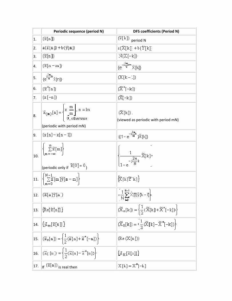
Periodic sequence (period N) DFS coefficients (Period N)

1.

period N

2.

3.

4.

5.

6.

7.

8.

(periodic with period mN)

(viewed as periodic with period mN)

9.

10.

(periodic only if )

11.

12.

13.

14.

15.

16.

17. If is real then

Table 6.1

Fourier Transform of periodic signals

If is periodic with period N, then we can write

Using equation (5.9) we see that

as is periodic with period N.

Example:

Consider the periodic impulse train

then

as only one term corresponding to n = 0 is non zero. Thus the DTFT is

Fourier Representation of Finite Duration sequence

The Discrete Fourier Transform (DFT)

We now consider the sequence such that and. Thus can be take non-

zero values only for. Such sequences are known as finite length sequences, and N is called the length

of the sequence. If a sequence has length M, we consider it to be a length N sequence where. In these

cases last ( N - M ) sample values are zero. To each finite length sequence of length N we can always

associate a periodic sequence defined by

(6.16)

Note that defined by equation (6.16) will always be a periodic sequence with period N,

whether is of finite length N or not. But when has finite length N, we can recover the

sequence from by defining

(6.17)

This is because of has finite length N , then there is no overlap between terms

and for different values of.

Recall that if

n = kN + r, where

then n modulo N = r ,

i.e. we add or subtract multiple of N from n until we get a number lying between 0 to N - 1. We will

use ((n))N to denote n modulo N. Then for finite length sequences of length N equation (6.16) can be

written as

(6.18)

We can extract from using equation (6.17). Thus there is one-to- one correspondance

between finite length sequences of length N , and periodic sequences of period N.

Given a finite length sequence we can associate a periodic sequence with it.

This periodic sequence has discrete Fourier series coefficients which are also periodic with

period N.From equations (6.2) and (6.3) we see that we need values of for

and for 0 = k = N - 1. Thus we define discrete Fourier transform of finite length

sequence as

where is DFS coefficient of associated periodic sequence. From we can get

by the relation.

then from this we can get using synthesis equation (6.2) and finally using equation

(6.17). In equations (6.2) and (6.3) summation interval is 0 to N - 1, we can write X [k ] directly in terms

of x[n], and x[n] directly in terms of X[k] as

For convenience of notation, we use the complex quantity

(6.19)

with this notation, DFT analysis and synthesis equations are written a follows

Analysis equation:

(6.20)

Synthesis equation:

(6.21)

If we use values of k and n outside the interval 0 to N - 1 in equation (6.20) and (6.21), then we will

not get values zero, but we will get periodic repetition of and respectively. In defining

DFT, we are concerned with values only in interval 0 to N - 1. Since a sequence of length M can also be

considered a sequence of length , we also specify the length of the sequence by saying N-

point-DFT, of sequence.

Sampling of the Fourier transform:

For sequence of length N, we have two kinds of representations, namely, discrete time

Fourier transform and discrete Fourier transform. The DFT values can be considered

as samples of

(as x[n] = 0 n < 0, for n < 0, and n > N - 1)

(6.22)

Thus is is obtained by sampling at.

Properties of the discrete Fourier transform

Since discrete Fourier transform is similar to the discrete Fourier series representation, the properties

are similar to DFS representation. We use the notation

to say that are DFT coefficient of finite length sequence.

1. Linearity

If two finite length sequence have length M and N , we can consider both of them with length greater

than or equal to maximum of M and N. Thus if

then

where all the DFTs are N-point DFT. This property follows directly from the equation (6.20)

2. Circular shift of a sequence

If we shift a finite length sequence of length N , we face some difficulties. When we shift it in

right direction the length of the sequence will becam according to

definition. Similarly if we shift it left , if may no longer be a finite length sequence

as may not be zero for n < 0. Since DFT coefficients are same as DFS coefficients, we define

a shift operation which looks like a shift of periodic sequence. From we get the periodic

sequence defined by

We can shift this sequence by m to get

Now we retain the first N values of this sequence

This operation is shown in figure below for m = 2, N = 5.

Fig 6.1

We can see that is not a shift of sequence. Using the propertiesof the modulo arithmetic we

have

and

(6.23)

The shift defined in equation (6.23) is known as circular shift. This is similar to a shift of sequence in a

circular register.

Fig 6.2

3. Shift property of DFT

From the definition of the circular shift, it is clear that it corresponds to linear shift of the associated

periodic sequence and so the shift property of the DFS coefficient will hold for the circular shift. Hence

(6.24)

and

(6.25)

4. Duality

We have the duality for the DFS coefficient given by , retaining one period of

the sequences the duality property for the DFT coefficient will become

5. Symmetry properties

We can infer all the symmetry properties of the DFT from the symmetry properties of the associated

periodic sequence and retaining the first period. Thus we have

and

We define conjugate symmetric and anti-symmetric points in the first period 0 to N - 1 by

Since

the above equation similar to

(6.26)

(6.27)

and are referred to as periodic conjugate symmetric and periodic conjugate anti-

symmetric parts of. In terms if these sequence the symmetric properties are

6. Circular convolution

We saw that multiplication of DFS coefficients corresponds of periodic convolution of the sequence.

Since DFT coefficients are DFS coefficients in the interval, , they will correspond to DFT of

the sequence retained by periodically convolving associated periodic sequences and retaining their first

period.

Periodic convolution is given by

using properties of the modulo arithmetic

and then

Since we get

The convolution defined by equation (6.28) is known as N-point-circular convolution of

sequence and , where both the sequence are considered sequence of length N. From

the periodic convolution property of DFS it is clear that DFT of is. If we use the

notation to denote the N point circular convolution we see that

(6.29)

In view of the duality property of the DFT we have

(6.30)

Properties of the Discrete Fourier transform are summarized in the table 6.2

Finite length sequence (length N) N-point DFT (length N)

1.

2.

3.

4.

5.

6.

7.

8.

9.

10.

11.

12.

13.

14. If is real sequence

Linear convolution using the Discrete Fourier Transform

Output of a linear time invariant-system is obtained by linear convolution of input signal with the

impulse response of the system. If we multiply DFT coefficients, and then take inverse transform we

will get circular convolution. From the examples it is clear that result of circular convolution is

different from the result of linear convolution of two sequences. But if we modify the two sequence

appropriately we can get the result of circular convolution to be same as linear convolution. Our

interest in doing linear convolution results form the fact that fast algorithms for computing DFT and

IDFT are available. These algorithms will be discussed in a later chapter. Here we show how we can

make result of circular convolution same as that of linear convolution.

If we have sequence of length L and a sequence of length M , the sequence

obtained by linear convolution has length ( L + M - 1).

This can be seen from the definition

(6.31)

as x[k] = 0 for. For hence. Similarly

for , so. Hence is possibly nonzero only for.

Now consider a sequence , DTFT is given by

writing

We get

If we take

we see that

Comparing this with the DFT equation (6.), we see that

can be seen as DFT coefficients of a sequence

(6.32)

obviously if has length less then or equal to N , then

However, if the length of

of l.

The sequence in equation (6.31) has the discrete Fourier transform

The N-point DFT of sequence is

where and are N

resulting as the inverse DFT of

From the circular convolution property of the DFT we have

Thus, the circular convolution of two

followed time aliasing, defined by equation (6.32). If N is greater than or equal to (

there will be no time aliasing as the linear convolu

we can use circular convolution for linear convolution by padding sufficient number of zeros at the

end of a finite length sequence. We can use DFT algorithm for calculating the circular convolution.

Definition of the Z-transform

We saw earlier that complex exponential of the from

We can generalize this for signals of the form

=

=

is greater than may not be equal to

in equation (6.31) has the discrete Fourier transform

sequence is

are N-point DFTs of and respectively. The sequence

is then by equation (6.32).

From the circular convolution property of the DFT we have

Thus, the circular convolution of two-finite length sequences can be viewed as linear convolution,

followed time aliasing, defined by equation (6.32). If N is greater than or equal to ( L +

there will be no time aliasing as the linear convolution produces a sequence of length (



We saw earlier that complex exponential of the from is an eigen function of for a LTI System.

We can generalize this for signals of the form where, is a complex number.

for all values

respectively. The sequence

finite length sequences can be viewed as linear convolution,

M - l ), then

tion produces a sequence of length ( L + M - l ). Thus



is an eigen function of for a LTI System.

=

=

where

Thus if the input signal is then output signal is. For

(7.1) is same as the discrete-time fourier transform. The

bilateral z-transform of the sequence. We define for any

where is a complex variable. Writing

and is angle of.

=

=

This shows that is Fourier transform of the sequence. When

reduces to the Fourier transform of. From equation (7.3) we see that for convergence of z

that Fourier transform of the sequence

others. The values of z - for which

the ROC contains unit circle (i.e.

converges. Following examples show that we must specify ROC to completely specify the z

Example 1: Let

=

=

This is a geometric series and converges if

then output signal is. For real (i.e for

time fourier transform. The in equation (7.1) is known as the

transform of the sequence. We define for any sequence of a sequence

is a complex variable. Writing in polar form we get , where

is Fourier transform of the sequence. When the z

to the Fourier transform of. From equation (7.3) we see that for convergence of z

that Fourier transform of the sequence converges. This will happen for some r and not for

is called the region of convergenc

the ROC contains unit circle (i.e. or equivalently then the Fourier transform also

converges. Following examples show that we must specify ROC to completely specify the z

, then

geometric series and converges if or. Then

(7.1)

), equation

in equation (7.1) is known as the

as

(7.2)

is magnitude

(7.3)

the z-transform

to the Fourier transform of. From equation (7.3) we see that for convergence of z-transform

converges. This will happen for some r and not for

is called the region of convergence(ROC). If

then the Fourier transform also

converges. Following examples show that we must specify ROC to completely specify the z-transform.

We see that at , and

zero of and value of where

of a region in Z-plane which lies outside the circle centered at origin and passing through the pole.

Example 2: Let,

=

=

This is a geometric series which converges when

, and at. Values of where is zero is called

where is zero is called a pole of. Here we see that ROC consists

outside the circle centered at origin and passing through the pole.

Fig 7.1

, then

This is a geometric series which converges when , that is Then

(7.4)

is zero is called

is zero is called a pole of. Here we see that ROC consists

outside the circle centered at origin and passing through the pole.

(7.5)

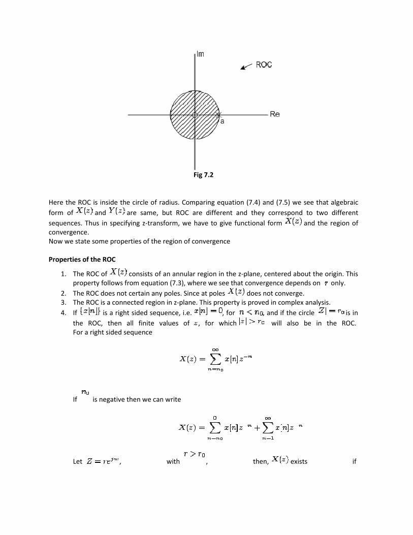
Here the ROC is inside the circle of

form of and are same, but ROC are different and they correspond to two different

sequences. Thus in specifying z-transform, we have to give functional form

convergence.

Now we state some properties of the region of convergence

Properties of the ROC

1. The ROC of consists of an annular region in the z

property follows from equation (7.3), where we see that convergence

2. The ROC does not certain any poles. Since at poles

3. The ROC is a connected region in z

4. If is a right sided sequence, i.e.

the ROC, then all finite values of

For a right sided sequence

If is negative then we can write

Let , with

Fig 7.2

Here the ROC is inside the circle of radius. Comparing equation (7.4) and (7.5) we see that algebraic

are same, but ROC are different and they correspond to two different

transform, we have to give functional form and the region of

Now we state some properties of the region of convergence

consists of an annular region in the z-plane, centered about the origin. This

property follows from equation (7.3), where we see that convergence depends on

The ROC does not certain any poles. Since at poles does not converge.

The ROC is a connected region in z-plane. This property is proved in complex analysis.

is a right sided sequence, i.e. , for , and if the circle

ROC, then all finite values of , for which will also be in the ROC.

is negative then we can write

, with , then, exists if

radius. Comparing equation (7.4) and (7.5) we see that algebraic

are same, but ROC are different and they correspond to two different

and the region of

plane, centered about the origin. This

depends on only.

plane. This property is proved in complex analysis.

, and if the circle is in

will also be in the ROC.

exists if

The first summation is finite as it consists of a finite number of terms. In the second

summation note that each term is less than

assumption that circle with radius

of z such that lies in ROC, except when. At

infinite. So if , i.e. the sequence

5. If is left sided sequence, i.e.

values of function

The proof is similar to the property 4. The point

purely

anticausal

6. If is non zero for,

and/or. In this case the

each term infinite which is the case when

if , and lies in the ROC if.

7. If is two-sided sequence and if circle

annular region in z-plane, which includes. We can express a two sided sequence as sum of a

right sided sequence and a left sided sequence. Then using property 4 and 5 we get this

property. Using

property 2 and 3 we see what ROC will be banded by circles passing

The inverse z-transform

The inverse z-transform is given by

the symbol indicates contour integration, over a counter clockwise contour in the ROC of. If

ratio of polynomials one can use Cauchy integral

alternative procedures also, which will be considered after discussing the properties of z

Properties of the z-transform

We use the notation

to denote z-transform of the sequence.

1. Linearity

is finite.

first summation is finite as it consists of a finite number of terms. In the second

summation note that each term is less than as. Since

assumption that circle with radius lies in ROC, the second sum is also finite. Hence values

lies in ROC, except when. At , the first summation will became

, i.e. the sequence is causal, the value will lie in the ROC.

is left sided sequence, i.e. and lies in the ROC, the

function also lie in the ROC.

The proof is similar to the property 4. The point , will lie in the ROC if the sequence is

, then ROC is entire z-plane except possibly

consists of finite number of terms and therefore it converges if

each term infinite which is the case when is different from 0 or.

lies in the ROC if.

sided sequence and if circle is in ROC, then ROC will consist of

plane, which includes. We can express a two sided sequence as sum of a


property. Using

property 2 and 3 we see what ROC will be banded by circles passing through the poles.

indicates contour integration, over a counter clockwise contour in the ROC of. If

ratio of polynomials one can use Cauchy integral theorem to calculate the contour integral. There are some other

alternative procedures also, which will be considered after discussing the properties of z

transform of the sequence.

is finite.

first summation is finite as it consists of a finite number of terms. In the second

is finite by our

lies in ROC, the second sum is also finite. Hence values

, the first summation will became

will lie in the ROC.

lies in the ROC, the

the ROC.

, will lie in the ROC if the sequence is

plane except possibly ,

of finite number of terms and therefore it converges if

lies in ROC,

is in ROC, then ROC will consist of

plane, which includes. We can express a two sided sequence as sum of a


property. Using

through the poles.

indicates contour integration, over a counter clockwise contour in the ROC of. If

theorem to calculate the contour integral. There are some other

alternative procedures also, which will be considered after discussing the properties of z-transform.

The z-transform of a linear combination of two sequence is given by

The algebraic form follows directly from the definition, equation (7.2). The linear combination is

such that some zero's can cancel the poles, then the region of convergence may be larger. For

example if the linear combination

entire z-plane except at , like individual ROCs are. If the intersection of

set, the z-transform of the linear combination will not exist.

2. Time shifting

If we shift the time sequence, we get

,

and/or

We have

changing variable,

=

=

=

The factor can affect the poles and zeros at

3. Multiplication by a exponential sequence

This follows directly from defining equation (7.2).

4. Differentiation of :

If we differentiate term by term we get

transform of a linear combination of two sequence is given by

ROC contains


's can cancel the poles, then the region of convergence may be larger. For

is a finite-length sequence, the ROC is

, like individual ROCs are. If the intersection of and

ransform of the linear combination will not exist.


except for possible addition or deletion of

the poles and zeros at ,

Multiplication by a exponential sequence

This follows directly from defining equation (7.2).

term by term we get


's can cancel the poles, then the region of convergence may be larger. For

length sequence, the ROC is

and is null


except for possible addition or deletion of

Thus

The ROC does not change (except

analytic function.

5. Conjugation of a complex sequence

=

=

=

Since ROC depends only an magnitude

6. Time Reversal

We have

putting

, except possibly

, ). This follows from the property that

5. Conjugation of a complex sequence

=

=

=

Since ROC depends only an magnitude it does not change.

). This follows from the property that is an

=

=

If we combine it with the previous property, we get

7. Convolution of sequence

The z-transform of the convolution is

Interchanging the order of summation

using time shifting property (or changing index of summation)

=

=

If there is pole-zero cancelation, the ROC will be larger than the common ROC of two sequence.

Convolution property plays an important role in analysis

produces a delay of , has the transfer function

depicted by

If we combine it with the previous property, we get

ROC contains

transform of the convolution is

of summation

using time shifting property (or changing index of summation)

zero cancelation, the ROC will be larger than the common ROC of two sequence.

Convolution property plays an important role in analysis of LTI system. An LTI system, which

, has the transfer function , therefore delay of

zero cancelation, the ROC will be larger than the common ROC of two sequence.

of LTI system. An LTI system, which

units is often

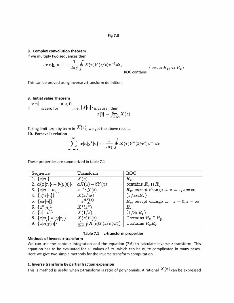
8. Complex convolution theorem

If we multiply two sequences then

This can be proved using inverse z-transform definition.

9. Initial value Theorem

If is zero for , i.e.

Taking limit term by term in , we get the above result.

10. Parseval's relation

These properties are summarized in table 7.1

Table

Methods of inverse z-transform

We can use the contour integration and the equation (7.6) to calculate inverse z

equation has to be evaluated for all values of

Here we give two simple methods for the inverse transform computation.

1. Inverse transform by partial fraction expansion

This is method is useful when z-transform is ratio of polynomials. A rational

Fig 7.3

ROC contains

transform definition.

is causal, then

, we get the above result.

These properties are summarized in table 7.1

Table 7.1 z-transform properties

We can use the contour integration and the equation (7.6) to calculate inverse z-transform. This

equation has to be evaluated for all values of , which can be quite complicated in many cases.

Here we give two simple methods for the inverse transform computation.

1. Inverse transform by partial fraction expansion

transform is ratio of polynomials. A rational can be expressed

transform. This

, which can be quite complicated in many cases.

can be expressed

as

where and are polynomials in. If degree

greater than or equal to the degree N of the denominator polynomial

by and re-express as

where the degree of polynomial

all poles are simple. Then

where

Example: Let

The partial fraction expression is

The inverse z-transform depends on the ROC. If ROC is

term is outside a circle(so that common ROC is outside a circle), sequences are causal. Using linearity

polynomials in. If degree of the numerator polynomial

greater than or equal to the degree N of the denominator polynomial , we can divide

is strictly less than that of. For simplicity let us assume that

=

=

=

=

transform depends on the ROC. If ROC is , then ROCs associated with each


of the numerator polynomial is

, we can divide

t us assume that

, then ROCs associated with each


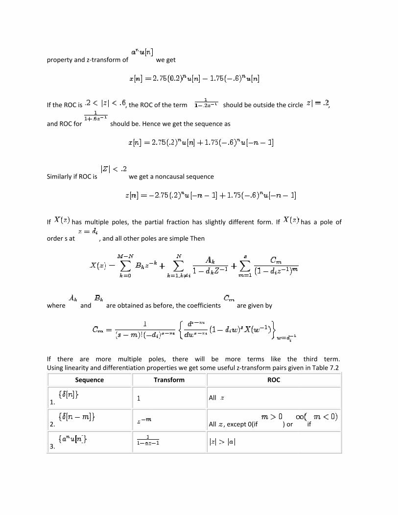
property and z-transform of

If the ROC is , the ROC of the term

and ROC for should be. Hence we get

Similarly if ROC is we get a noncausal sequence

If has multiple poles, the partial fraction has slightly different form. If

order s at , and all other poles are simple Then

where and are obtained as before, the coefficients

If there are more multiple poles, there will be more terms like the third term.

Using linearity and differentiation properties we get some useful z

Sequence

1.

2.

3.

we get

, the ROC of the term should be outside the circle

should be. Hence we get the sequence as

we get a noncausal sequence

has multiple poles, the partial fraction has slightly different form. If

, and all other poles are simple Then

are obtained as before, the coefficients are given by


Using linearity and differentiation properties we get some useful z-transform pairs given in Table 7.2

Transform ROC

All

All , except 0(if ) or

should be outside the circle ,

has a pole of


transform pairs given in Table 7.2

if

4.

5.

6.

7.

8.

9.

Table 7.2

2. Inverse Transform via long division

For causal sequence the z-transform

expansion, the coefficient multiplying the term

terms of poles of.

Example 1: Let

This is a causal sequence, long division gives

Table 7.2 Some useful z-transform pairs

Inverse Transform via long division

transform can be exported into a pure series in. In the series

expansion, the coefficient multiplying the term is. If is anticausal then we expand in


can be exported into a pure series in. In the series

is anticausal then we expand in


This gi

We can see that it is not easy to write the

Example 2:

Using the pure series expansion for

=

=

Analysis of LTI system using z-transform

From the convolution property we have

where are are

and impulse response respectively. The

function of the system. For on the unit circle

response of the system, provided th

A causal LTI system has impulse response

in z-plane including. Thus a discrete time LTI system is causal if and only if ROC is exterior of a circle

which includes infinit

An LTI system is stable if and only if impulse response

equivalent to saying that unit circle is in the ROC of.

For a causal and stable system ROC is outside a circle and ROC contains the unit circle. That means all

the poles are inside the unit circle. Thus a causal LTI system is stable if and if only if all the poles

inside unit circle.

LTI systems characterized by Linear constant coefficient difference equation

For the system characterized by

We take the z-transform of both sides and use linearity and the time shift property to get

This gives

We can see that it is not easy to write the

Using the pure series expansion for with , we obtain

transform

From the convolution property we have

z-transforms of input sequence , output sequence

respectively. The is referred to as system function or transfer

on the unit circle , reduces to the frequency

response of the system, provided that unit circle is in the ROC for.

A causal LTI system has impulse response such that. Thus ROC of is exterior of a circle

plane including. Thus a discrete time LTI system is causal if and only if ROC is exterior of a circle

which includes infinit

An LTI system is stable if and only if impulse response is absolutely summable. This is



he poles are inside the unit circle. Thus a causal LTI system is stable if and if only if all the poles

LTI systems characterized by Linear constant coefficient difference equation

transform of both sides and use linearity and the time shift property to get

,.....

We can see that it is not easy to write the term.

, output sequence

is referred to as system function or transfer

reduces to the frequency

at unit circle is in the ROC for.

is exterior of a circle

plane including. Thus a discrete time LTI system is causal if and only if ROC is exterior of a circle

which includes infinity.

is absolutely summable. This is



he poles are inside the unit circle. Thus a causal LTI system is stable if and if only if all the poles

transform of both sides and use linearity and the time shift property to get

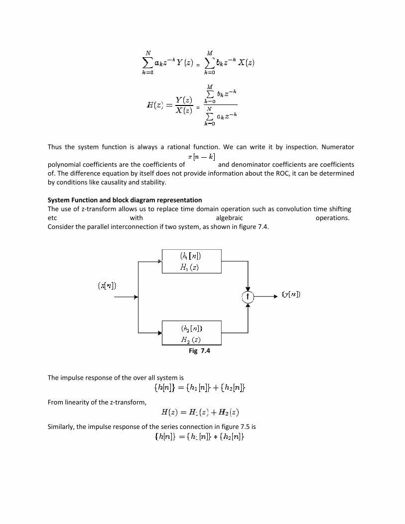
Thus the system function is always a rational function. We can write it by inspection. Numerator

polynomial coefficients are the coefficients of

of. The difference equation by itself does not provide information about the ROC, it can be determined

by conditions like causality and stability.

System Function and block diagram representation

The use of z-transform allows us to replace time domain operation such as convolution time shifting

etc with algebraic operations.

Consider the parallel interconnection if two system, as shown in figure 7.4.

The impulse response of the over all

From linearity of the z-transform,

Similarly, the impulse response of the series connection in figure 7.5 is

=

=


polynomial coefficients are the coefficients of and denominator coefficients are coefficients


by conditions like causality and stability.

System Function and block diagram representation

transform allows us to replace time domain operation such as convolution time shifting


Consider the parallel interconnection if two system, as shown in figure 7.4.

Fig 7.4

The impulse response of the over all system is

Similarly, the impulse response of the series connection in figure 7.5 is


and denominator coefficients are coefficients


transform allows us to replace time domain operation such as convolution time shifting


From the convolution property.

The z-transform of the interconnection of linear system can be obtained by algebraic

example consider the feed back connection in figure 7.6

We have

or

Even though this course is primarily about the discrete time signal processing, most signals we

encounter in daily life are continuous in time such as speech, music and images. Increasingly discrete

time signals processing algorithms are being used to process such signals. For processing by digital

systems, the discrete time signals are represented in digital form with

binary word. Therefore we need the analog to digital and digital to analog interface circuits to convert

the continuous time signals into discrete time digital form and vice versa. As a result it is necessary to

develop the relations between continuous time and discrete time representations.

Fig 7.5

transform of the interconnection of linear system can be obtained by algebraic

example consider the feed back connection in figure 7.6

Fig 7.6

=

=

=

=

=


life are continuous in time such as speech, music and images. Increasingly discrete


systems, the discrete time signals are represented in digital form with each discrete time sample as



lations between continuous time and discrete time representations.

transform of the interconnection of linear system can be obtained by algebraic means. For


life are continuous in time such as speech, music and images. Increasingly discrete-


each discrete time sample as



Sampling of continuous time signals

Let be a continuous time signal that is sampled uniformly at t = nT generating the

sequence where

T is called sampling period, the reciprocal of T is called the sampling frequency. The frequency domain

representation of is given by its Fourier transform

where the frequency-domain representation of is given by its discrete time fourier transform

To establish relationship between the two representation, we use impulse train sampling. This should

be understood as mathematically convenient method for understanding sampling. Actual circuits can

not produce continuous time impulses. A periodic impulse train is given by

(8.1)

Fig 8.1

(8.2)

using sampling property of the impulse , we get

(8.3)

Fig 8.2

From multiplication property, we know that

The Fourier transform of a impulse train is given by

where

Using the property that it follows that

(8.4)

Thus is a periodic function of with period , consisting of superposition of shifted

replicas of scaled by. Figure 8.3 illustrates this for two cases.

Fig 8.3

If or equivalently there is no overlap between shifted replicas

of , where as with , there is overlap. Thus if is faithfully

replicated in and can be recovered from by means of lowpass filtering with gain T

and cut off frequency between and. This result is known as Nyquist sampling theorem.

Sampling Theorem

Let be a bandlimited signal with , for. Then is uniquely determined by its

samples , if

The frequency is called Nyquist rate, while the frequency is called the Nyquist frequency.

The signal can be reconstructed by passing through a lowpass filter.

Fig 8.4

The impulse response of this filter is

(8.5)

Assuming we get

(8.6)

The above expression (8.5) shows that reconstructed continuous time signal is obtained by

shifting in time the impulse response of low pass filter by an amount nT and scaling it in

amplitude by a factor for all integer values n. The interpolation using the impulse

response of an ideal low pass filter in (8.6) is referred to as bandlimited interpolation, since it

implements reconstruction if is bandlimited and sampling frequency satisfies the condition of

the sampling theorem. The reconstruction is in the mean square sense i.e.

The effect of underselling: Aliasing

We have seen earlier that spectrum is not faithfully copied when. The terms in (8.4)

overlap. The signal is no longer recoverable from. This effect, in which individual terms in

equation (8.4) overlap is called aliasing.

For the ideal low pass signal

Hence

Thus at the sampling instants the signal values of the original and reconstructed signal are same for

any sampling frequency.

DTFT of the discrete time signal

Taking continuous time Fourier transform of equation (8.3) we get

(8.7)

Since , we get the DTFT

(8.8)

comparing them we see that

using equation (8.4) we get

or

(8.9)

Comparing equation (8.4) and(8.9) we see that is simply a frequency scaled version

of with frequency scaling specified by. This can be thought of as a normalization of

frequency axis so that frequency in is normalized to in. For the example

in figure 8.3 the is shown in figure (8.5)

From equation (8.5) we see that

Fig 8.5

(8.10)

We refer to the system that implements as ideal continuous-to-discrete time (C/D)

convertor and is depicted in figure (8.6)

Fig 8.6

The ideal system that takes sequence as input and produces given equation (8.5) is

called ideal discrete to continuous time convertor and is depicted in Figure (8.7)

Fig 8.7

Discrete time processing of continuous time signal

Figure (8.8) shows a system for discrete time processing of continuous time system

Fig 8.8

The over all system has as input and as output. We have the following relations among

the signals.

and

If the discrete time system is LTI then we have

combining these equations we get

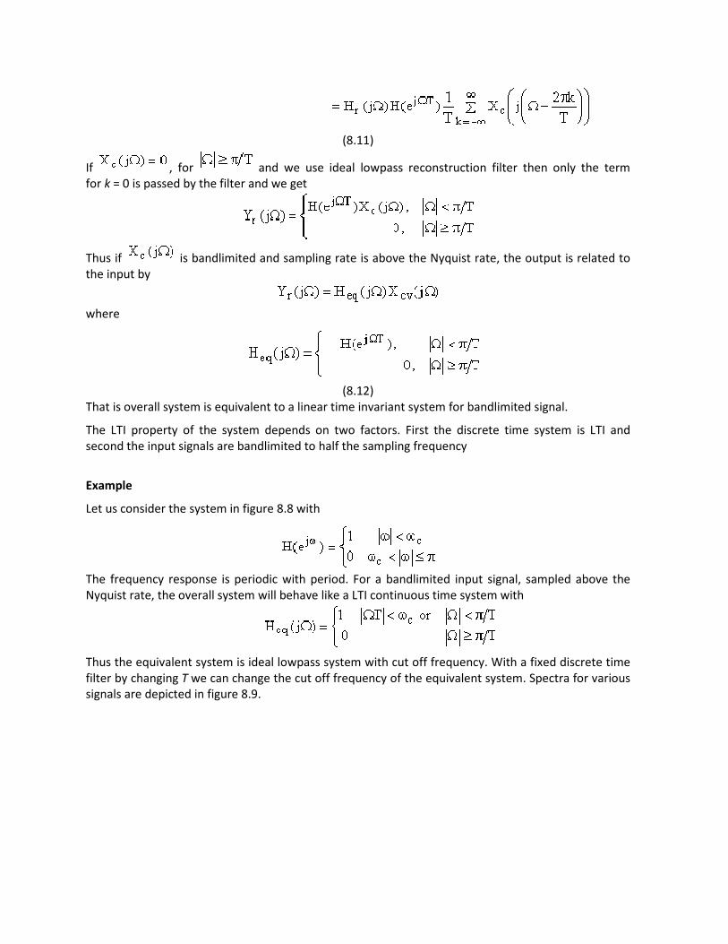
(8.11)

If , for and we use ideal lowpass reconstruction filter then only the term

for k = 0 is passed by the filter and we get

Thus if is bandlimited and sampling rate is above the Nyquist rate, the output is related to

the input by

where

(8.12)

That is overall system is equivalent to a linear time invariant system for bandlimited signal.

The LTI property of the system depends on two factors. First the discrete time system is LTI and

second the input signals are bandlimited to half the sampling frequency

Example

Let us consider the system in figure 8.8 with

The frequency response is periodic with period. For a bandlimited input signal, sampled above the

Nyquist rate, the overall system will behave like a LTI continuous time system with

Thus the equivalent system is ideal lowpass system with cut off frequency. With a fixed discrete time

filter by changing T we can change the cut off frequency of the equivalent system. Spectra for various

signals are depicted in figure 8.9.

FIGURE 8.9

From figure (8.9) we can see that ever if there is same aliasing due to sampling, if the components are

filtered out by the discrete time system, the over all transfer function will remain same. Thus the

requirement is

instead of for no aliasing.

Continuous time processing of discrete time signals

Consider the system shown in figure (8.10)

Figure 8.10

We have

Therefore the overall system behaves as a discrete time system where frequency response is

(8.13)

Example

Let us consider a discrete time system with frequency response

when is an integer, this system is delay by

but when is not an integer, we can not write the above equation. Suppose that we implement this

using system in figure (8.10). Then we have

(8.14)

So that overall system has frequency response. The equation (8.13) represents a time delay secs

in continuous time whether is integer or not, thus

The signal is bandlimited interpolation of and is obtained by sampling. Thus y[n]

are samples of band limited signal delayed by.

For are depicted in figure (8.11)

Fig 8.11

Sampling of discrete time Signals

In analogy with continuous time sampling, the sampling of a discrete time signal can be represented

as shown in figure 8.12

FIGURE 8.12

(8.15)

In frequency domain, we get

The Fourier transform of sequence is

where

Thus we get

(8.16)

Figure 8.13 illustrates signals and their spectra

FIGURE 8.13

If or equivalently or there will be no aliasing (i.e non zero

portions of do not overlap) and the signal can be recovered from by passing

through an ideal low-pass filter with gain equal to N and cut off equal to

FIGURE 8.14

If , there will be aliasing, and so will be different from. However as in continuous

time case

independently of whether there is aliasing or not.

For ideal low pass filter

with we get

Discrete time decimation and interpolation

The sampled signal in equation (8.13) has ( N - 1) samples out of every N samples as zeros. We define

a new sequence which retains only the non zero values

(8.17)

this is called a decimated sequence, whatever may be the value of. The DTFT of the decimated

request is given by

since only for multiples of has non zero value,

(8.18)

For the signal shown in figure (8.13) the sequence and its spectrum are illustrated in figure

(8.15)

Fig 8.15

If the original signal was obtained by sampling a continuous time signal, the process of

decimation can be viewed as reduction in the sampling rate by a factor of N. With this interpretation,

the process of decimationis often referred as down sampling. The block diagram for this is shown in

figure (8.16)

Fig 8.16

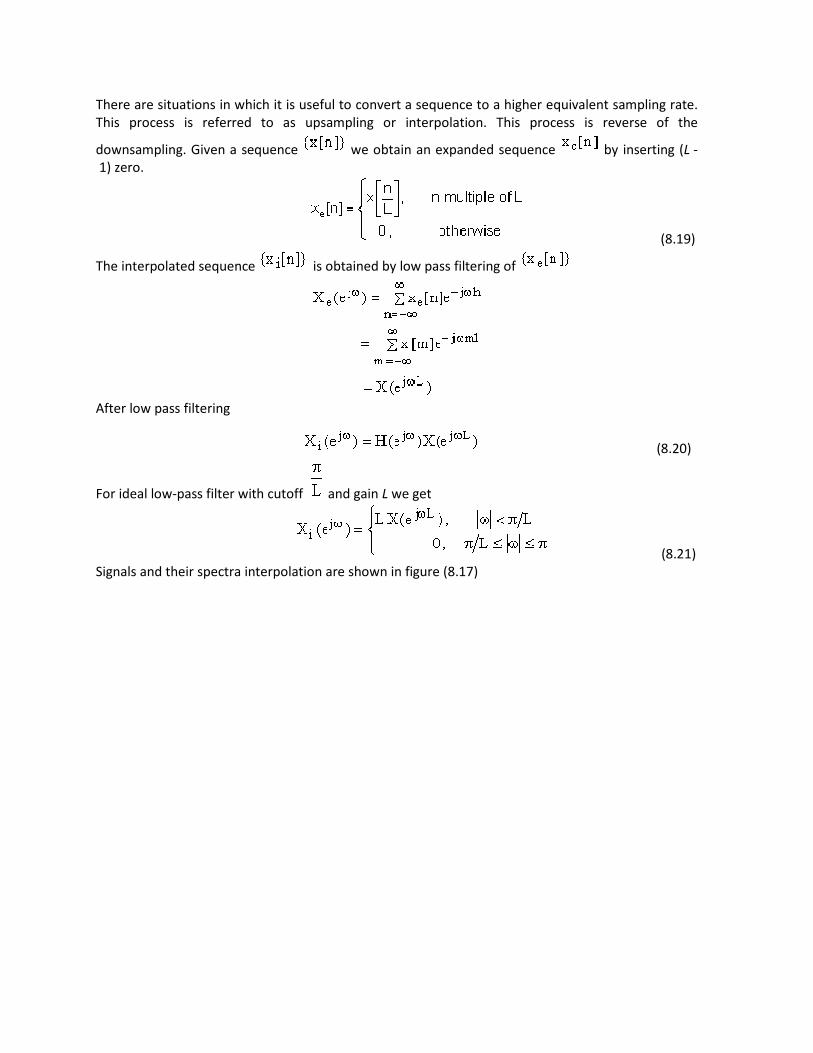
There are situations in which it is useful to convert a sequence to a higher equivalent sampling rate.

This process is referred to as upsampling or interpolation. This process is reverse of the

downsampling. Given a sequence we obtain an expanded sequence by inserting (L -

1) zero.

(8.19)

The interpolated sequence is obtained by low pass filtering of

After low pass filtering

(8.20)

For ideal low-pass filter with cutoff and gain L we get

(8.21)

Signals and their spectra interpolation are shown in figure (8.17)

Fig 8.17

We can get a non integer change in rate if it is ratio of two integers by using upsampling and

downsampling operations.

In many applications of signal processing we want to change the relative amplitudes and frequency

contents of a signal. This process is generally referred to as filtering. Since the Fourier transform of

the output is product of input Fourier transform and frequency response of the system, we have to

use appropriate frequency response.

Ideal frequency selective filters

An ideal frequency reflective filter passes complex exponential signal. for a given set of frequencies

and completely rejects the others. Figure (9.1) shows frequency response for ideal low pass filter

(LPF), ideal high pass filter (HPF), ideal bandpass filter (BPF) and ideal backstop filter (BSF).

Fig 9.1

The ideal filters have a frequency response that is real and non-negative, in other words, has a zero

phase characteristics. A linear phase characteristics introduces a time shift and this causes no

distortion in the shape of the signal in the passband.

Since the Fourier transfer of a stable impulse response is continuous function of , can not get a

stable ideal filter.

Filter specification

Since the frequency response of the realizable filter should be a continuous function, the magnitude response of a

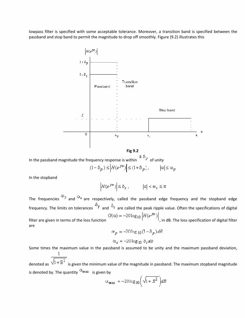
lowpass filter is specified with some acceptable tolerance. Moreover, a transition band is specified between the

passband and stop band to permit the magnitude to drop off smoothly. Figure (9.2) illustrates this

Fig 9.2

In the passband magnitude the frequency response is within of unity

In the stopband

The frequencies and are respectively, called the passband edge frequency and the stopband edge

frequency. The limits on tolerances and are called the peak ripple value. Often the specifications of digital

filter are given in terms of the loss function , in dB. The loss specification of digital filter

are

Some times the maximum value in the passband is assumed to be unity and the maximum passband deviation,

denoted as is given the minimum value of the magnitude in passband. The maximum stopband magnitude

is denoted by. The quantity is given by

These are illustrated in Fig(9.3)

Fig 9.3

If the phase response is not specified, one prefers to use IIR digital filter. In case of an IIR filter design, the most

common practice is to convert the digital filter specifications to analog low pass prototype filter specifications, to

determine the analog low pass transfer function meeting these specifications, and then to transform it into

desired digital filter transfer function. This methods is used for the following reasons:

1. Analog filter approximation techniques are highly advanced.

2. They usually yield closed form solutions.

3. Extensive tables are available for analog-design.

4. Many applications require the digital solutions of analog filters.

The transformations generally have two properties (1) the imaginary axis of the s-plane maps into unit circle of the

z-plane and (2) a stable continuous time filter is transformed to a stable discrete time filter.

Filter design by impulse invariance

In the impulse variance design procedure the impulse response of the impulse response of

the discrete time system is proportional to equally spaced samples of the continues time filter, i.e.,

where Td represents a sampling interval, since the specifications of the filter are given in discrete time

domain, it turns out that Td has no role to play in design of the filter. From the sampling theorem we

know that the frequency response of the discrete time filter is given by

Since any practical continuous time filter is not strictly bandlimited there issome aliasing. However, if

the continuous time filter approaches zero at high frequencies, the aliasing may be negligible. Then

the frequency response of the discrete time filter is

We first convert digital filter specifications to continuous time filter specifications. Neglecting aliasing,

we get specification by applying the relation

(9.2)

where is transferred to the designed filter H(z), we again use equation (9.2) and the

parameter Tdcancels out.

Let us assume that the poles of the continuous time filter are simple, then

The corresponding impulse response is

Then

The system function for this is

We see that a pole at in the s-plane is transformed to a pole at Td in the z-plane. If

the continuous time filter is stable, that is , then the magnitude of will be less

than 1, so the pole will be inside unit circle. Thus the causal discrete time filter is stable. The mapping

of zeros is not so straight forward.

Example:

Design a lowpass IIR digital filter H(z) with maximally flat magnitude characteristics. The passband

edge frequency is with a passband ripple not exceeding 0.5dB. The minimum stopband

attenuation at the stopband edge frequency of is 15 dB.

We assume that no aliasing occurs. Taking , the analog filter has ,

the passband ripple is 0.5dB, and minimum stopped attenuation is 15dB. For maximally flat frequency

response we choose Butterworth filter characteristics. From passband ripple of 0.5 dB we get

at passband edge.

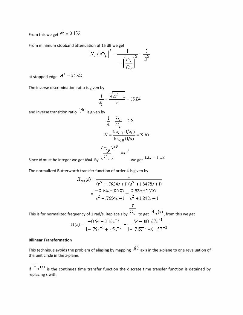
From this we get

From minimum stopband attenuation of 15 dB we get

at stopped edge

The inverse discrimination ratio is given by

and inverse transition ratio is given by

Since N must be integer we get N=4. By we get

The normalized Butterworth transfer function of order 4 is given by

This is for normalized frequency of 1 rad/s. Replace s by to get , from this we get

Bilinear Transformation

This technique avoids the problem of aliasing by mapping axis in the s-plane to one revaluation of

the unit circle in the z-plane.

If is the continues time transfer function the discrete time transfer function is detained by

replacing s with

(9.3)

Rearranging terms in equation (9.3) we obtain.

Substituting , we get

If , it is then magnitude of the real part in denominator is more than that of the numerator and

so. Similarly if , than for all. Thus poles in the left half of the s-plane will get mapped to

the poles inside the unit circle in z-plane. If then

So, , writing we get

rearranging we get

or

(9.5)

or

(9.6)

The compression of frequency axis represented by (9.5) is nonlinear. This is illustrated in figure 9.4.

Fig 9.4

Because of the nonlinear compression of the frequency axis, there is considerable phase distortion in

the bilinear transformation.

Example

We use the specifications given in the previous example. Using equation (9.5) with we get

Some frequently used analog filters

In the previous two examples we have used Butterworth filter. The Butterworth filter of order n is

described by the magnitude square frequency response of

It has the following properties

1.

2.

3. is monotonically decreasing function of

4. As n gets larger, approaches an ideal low pass filter

5. is called maximally flat at origin, since all order derivative exist and they are zero

at

The poles of a Butterworth filter lie on circle of radius in s-plane.

There are two types of Chebyshev filters, one containing ripples in the passband (type I) and the other

containing a ripple in the stopband (type II). A Type I low pass normalizer Chebyshev filter has the

magnitude squared frequency response.

where is nth

order Chebyshev polynomial. We have the relationship

with

Chebyshev filters have the following properties

1. The magnitude squared frequency response oscillates between 1 and within the

passband, the so called equiripple and has a value of at , the normalized cut

off frequency.

2. The magnitude response is monotonic outside the passband including transitionand stopband.

3. The poles of the Chebysher filter lie on an ellipse in s-plane.

An elliptic filter has ripples both in passband and in stopband. The square magnitude frequency

response is given by

where is Chebyshev rational function of O determined from specified ripple characteristics.

An nth

order Chebyshev filter has sharper cutoff than a Butterworth filter, that is, has a narrower

transition bandwidth. Elliptic filter provides the smallest transition width.

Design of Digital filter using Digital to Digital transformation

There exists a set of transformation that takes a low pass digital filter and turn into highpass,

bandpass, bandstop or another lowpass digital filter. These transformations are given in table 9.1.

The transformations all take the form of replacing the in by some function of.

Type From To Transformation Design Formula

Low pass

cutoff

Low pass

cutoff

LPF HPF

LPF BPF

LPF BSF

Starting with a set of digital specifications and using the inverse of the design equation given in table

9.1, a set of lowpass digital requirements can be established. A LPF digital prototype filter is

then selected to satisfy these requirements and the proper digital to digital transformation is applied

to give the desired.

Example

Using the digital to digital transformation, find the system function for a low-pass digital filter

that satisfies the following set the requirements (a) monotone stop and passband (b)-3dB cutoff

frequency of (c) attenuation at and past is at least 15dB.

Because of monotone requirement, a Butterworth filter is selected. The required n is given by

rounded to 2.

For we get from table 9.1. , From standard tables (or MATLAB) we find

standard 2 nd order Butterworth filter with cut off and then apply the digital transform to get

FIR filter design

In the previous section, digital filters were designed to give a desired frequency response magnitude

without regard to the phase response. In many cases a linear phase characteristics is required through

the passband of the filter. It can be shown that causal IIR filter cannot produce a linear phase

characteristics and only special forms of causal FIR filters can give linear phase.

If represents the impulse response of a discrete time linear system a necessary and sufficient

condition for linear phase is that have finite duration N , that it be symmetric about its mid

point, i.e.

For N even, we get

For N odd

For N even we get a non-integer delay, which will cause the value of the sequenceto change, [See

continuous time implementation of discrete time system, for interpretation of non-integer delay].

One approach to design FIR filters with linear phase is to use windowing.

The easiest way to obtain an FIR filter is to simply truncate the impulse response of an IIR filter.

If is the impulse response of the designed FIR filter, then an FIR filter with

impulseresponse can be obtained as follows.

This can be thought of as being formed by a product of and a window function

where is said to be rectangular window and is given by

Using modulation property of Fourier transfer

For example if is ideal low pass filter and is rectangular window is measured version

of the ideal low pass frequency response.

Fig 9.5

In general, the index the main lobe of , the more spreading where as the narrower

the main lobe (larger N), the closer comes to. In general, we are left with a trade-off of

making N large-enough so that smearing is minimized, yet small enough to allow reasonable

implementation. Much work has been done on adjusting to satisfy certain main lobe and side

lobe requirements. Some of the commonly used windows are give in below.

(a) Rectangular

(b) Bartlett (or triangle)

(c) Hanning

(d) Harming

(e) Blackman

(f) Kaiser

where is modified zero-order Bessel function of the first kind given by

The main lobe width and first side lobe attenuation increase as we proceed down the window listed

above.

An ideal lowpass filter with linear phase and cut off is characterized by

The corresponding impulse response is

Since this is symmetric about , if we change and use one of the windows listed

above the will get linear phase FIR filter. Transition width and minimum stopped attenuation are listed

in the Table 9.3.

Window Transition Width Minimum stopband

attenuation

Rectangular

-21db

Bartlett

-25dB

Hanning

-44dB

Hamming

-53dB

Blackman

-74dB

Kaiser variable variable

Table 9.3

We first choose a window that satisfies the minimum attenuation. The transition bandwidth is

approximately that allows us to choose the value of N. Actual frequency response characteristic are

then calculated and we see if the requirements are met or not. Accordingly N is adjusted parameters

for kaiser window are obtained from design formula available for this MATLAB or similar programmes

have all there formulas.

Realizations of Digital Filters

We have many realizations of digital filter. Some of these are now discussed. Direct Form Realization -

An important class of linear time -invariant systems is characterized by the transfer function.

A system with input and output could be realized by the following constant coefficient

difference equation

A realization of the filter using equation (9.31) is shown in figure (9.6)

Fig 9.6 Direct form I

The output is seen to be weighted sum of input and past inputs and

past outputs. Another realization can be obtained by uniting as product of two transfer

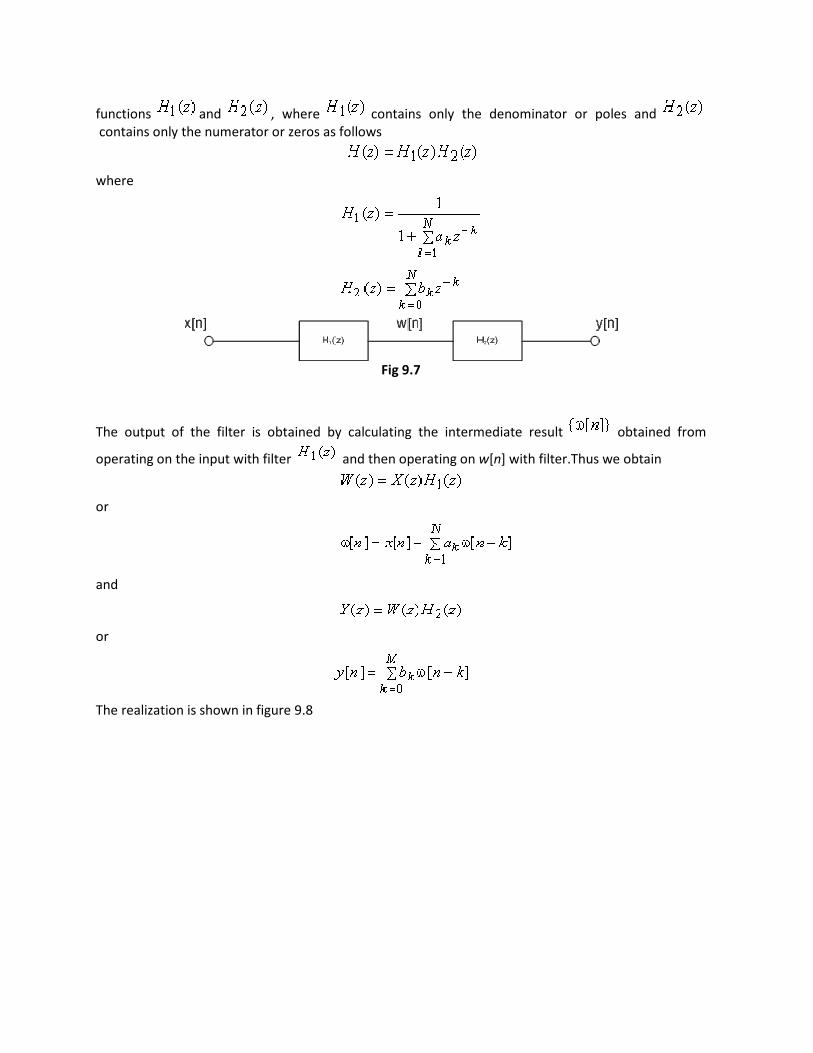
functions and , where contains only the denominator or poles and

contains only the numerator or zeros as follows

where

Fig 9.7

The output of the filter is obtained by calculating the intermediate result obtained from

operating on the input with filter and then operating on w[n] with filter.Thus we obtain

or

and

or

The realization is shown in figure 9.8

Fig 9.8

Upon close examination of Fig 9.8, it can be seen that the two branches of delay elements can be

combined as they both refer to delayed versions of and upon simplification, the direct form II

canonical realization is obtained as shown in figure 9.9.

Fig 9.9 Direct form II

In this form the number of delay element is max (M,N). It can be shown that this is the minimum

number of delay elements that are required to implement the digital filter. This does not mean that

this is the best realization. Immunity to roundoff and quantization are very important considerations.

An important special case that is used as building block occurs when. Thus is ratio of two

qualities in , called biquadratic section, and is given by

The alternative form is found to be useful for amplitude scaling for improving performance file filter

operation. This form is shown in figure 9.10.

Fig 9.10

Cascade Realizations: In the cascade realization is broken into productof transfer

functions each a rational expression in as follows

Fig 9.11

could be broken up in many ways; however the most common method is to use biquadratic

sections. Thus

by letting and equal to zero we get bilinear section. Even among the biquadratic sections

we have many choices as how we pair poles and zeros. Also the order of the sections can be different

Example:

Final cascade realization of

Using only real coefficients can be decompressed as

Divides both numerator and denominator by and factoring 8 as , one possible

rearrangement for is

This can be realized as shown is figure 9.12

Fig 9.12

Parallel Realizations:

The transfer function H ( z ) could be written as a sum of transfer functions

as follows:

One parallel form results when are all selected to be of the following form for

If , we will have a section of FIR filter, obtained by performing long division. Once

denominator polynomial has degree more than the numerator polynomial we perform the partial

fraction expansion. The resulting structure is shown in figure 9.13.

Fig 9.13

Example:Find the parallel form for the filter given in last example.

Using MATLAB program or otherwise we get

using direst form realization for individual section we get the structure shown in figure 9.14.

Fig 9.14 Apart from these there exist a number of other realizations like lattice form, state variable

realization etc.

digital signal processing - biher · system the solutions are obtained in real time ... notation...

Documents