Digital Hydraulic Actuator Study

Phase III jFinal Report

Sponsored by:Air Programs, Office of Naval Research

Contract Nonr 4375(00)

iBy:

G. W. Scott

DCIBM NO.: 66-L03-005

U A 1967AAR

Reproduction of this report in whole orin part is permitted for any purpose ofthe United States Government.

Distribution of this document is unlimnited.

ýMK Electronics Systems Center, Owego, Now York

NovemLer 1966

]II

DIGITAL HYDRAULIC ACTUATOR STUDY

aPhase Mi

Final ReportISponsored By

Air Programs, Office of Naval ResearchContract Nonr 4375(00)

IByI G.W. Scott

IIBM No: 66- L03-005!November 1966

Reproduction of this report in whole orin part is permitted for any purpose ofthe United States Government.

Distribution of this document is unlimited.

tFederal Systems Division, Electronics Systems Center,~S~) ~Owvego, Newý York

ft ABSTRACT

To further support the practicability of the digital hydraulic actuatoras a control component, IBM has successfully demonstrated operation of thePhase MI laboratory model in a simulated digital flight control system. Per-formance using the laboratory model is compared with the performance whenusi4 a mathematical model. Recorded transients and the values obtained fora maximum stable step and gain change are presented. The effect of varyingthe actuator parameters and the validity of a linearized model is also estab-lished. Agreement of the results shows the mathematical model to accuratelyrepresent the actual hardware. Hence, this study verified the results of bothPhase I and Phase H.

II

ACKNOWLEDGEMENTS

Mr. J. W. Raider, the originator of the digital hydraulic concept in-vestigated, ulgnlficantly contributed to the success of this program by hisparticipation during the initial part of Phase MI and the earlier phases.

The mathematical model and simulated flight control system was pro-gramnmed by Mr. N. L. Pleszkoch.

iv

i

TABLE OF CONTENTS

Section Page

ABSTRACT ................................ iii

ACKNOWLEDGEMENTS ........................ iv

I INTRODUCTION ............................. 1-1

A. SUMMARY ............................. 1-1

B. PURPOSE AND OBJECTIVES OF PROGRAM ....... 1-1

C. DESCRIPTION ........................... 1-2

D. CONCLUSIONS .......................... 1-5

E. RECOMMENDATIONS....................... 1-5

H TECHNICAL APPROACH ....................... 2-1

j A. EQUIPMENT - ARRANGEMENT ANDDESCRIPTION ......................... 2-2

1. Valve Control Logic ....................... 2-22. Position Control Logic ..................... 2-43. Digital Hydraulic Actuator ................ 2-44. Coulomb Friction .......................... 2-6

B. METHOD OF SIMULATION .................. 2-6

1. Digital Autopilot ...................... 2-6

2. Digital Hydraulic Actuator (Digital Portion) 2-113. Digital Hydraulic Actuator (Analog Portion) .... 2-15tj 4. Comparison ......................... 2-17

A

Table of Contents (cont)

Section Page

mI MATHEMATICAL MODEL EVALUATIOn................ 3-1

A. PARAMETER VALUES ....................... 3-1

B. RESULTS ................................. 3-4

1. Effect of the Parameter C................... 3-92. Effect of the Parameter 6/V ............... 3-103. Gain-Phaue ........................... 3-14

IV DIGITAL FLIGHT CONTROL SIMULATION .............. 4-1

A. DESCRIPTION ............................. 4-1

B. RESULTS ................................. 4-1

1. Effect of Leakage Parameters ............. 4-12. Effect of Compensation Gain, K ... 4-83. Comparison with Analog Flight Control ........ 4-84. Gain-Phase ............................ 4-8

V LINEARIZED MODEL .......................... 5-1

A. DEVELOPMENT ......................... 5-1

B. RESULTS .............................. 5-4

REFERENCES 5-5

APPENDIX Title A-1

A DIGITAL HYDRAULIC ACTUATOR OPERATIONALCONCEPT ............................. A-1

B CIRCUITS CONTROL LOGIC .................. B-1

C LIST OF SYMBOLS ........................ C-I

D DISTRIBUTION LIST-NONR 4375(00) .............. D-I

vi

LIST OF ILLUSTRATIONS

jFigure Title Page

1-1 Simulation Arrangement ..................... 1-3j 1-2 Laboratory Arrangement..................... 1-4

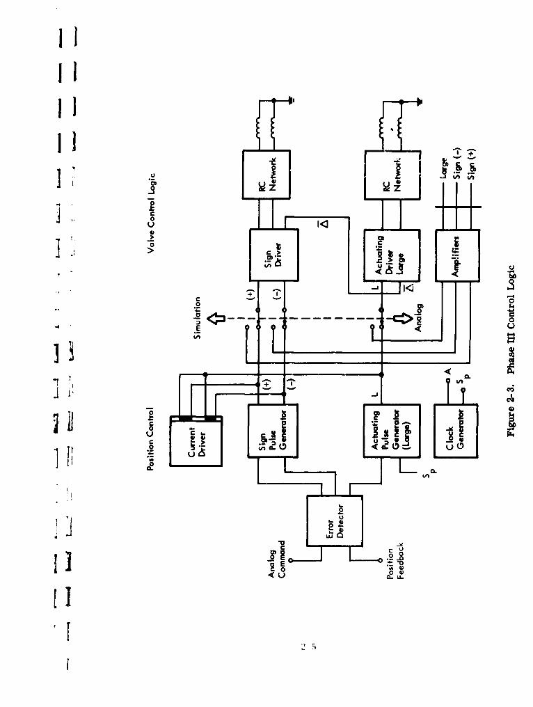
2-1 Arrangement of Equipment ..................... 2-32-2 Flow Curve for Digital Unit ................... 2-42-3 Phase MI Control Logic ...................... 2-52-4 Mathematical Model of Digital Autopilot,

Digital Actuator, and Missile Dynamics ......... 2-72-5 Digital Autopilot ........................... 2-82-6 Pulse Logic ................................. 2-92-7 Flow Calculations ........................... 2-112-8 Timing Chart ............................... 2-132-9 Digital Integration ......................... 2-142-10 Method of Obtaining Limiting Values for the

Digital Integrator .......................... 2-152-11 Actuator Dynamics ........................... 2-162-12 Simulation of Coulomb Friction (Phase I) .......... 2-162-13 Simulation of Coulomb Friction (Phase M) ......... 2-172-14 Recorded Transients for 4r = "1/2° Run 207

Table 2-1 ............................. 2-19

53-1 Recorded Motion of Ram with Digital HydraulicActuator in Simulated Control loop (AF = 60 lbs)... 3-6

3-2 Ram Motion for a Yaw Step Command (N =10) ..... .. 3-73-3 Simulation Arrangement ....................... 3-83-4 Block Diagram for DHA Load Dynamics ............. 3-93-5 Recorded Transients Showing Actual Motion of

Digital Hydraulic Actuator and the Motio.a Gen-erated with the Mathematical Model ............ 3-10

3-6 Recorded Transients for a Yaw Step Command(N = 10) Using Mathematical Model ............ 3-11

3-7 Limi Cycle Generated with the MathematicalModel in the Simulated Control System .......... 3-11

3-8 Recorded Transients for a Yaw Step Command(NY = 10) Using Actual Hardware withMathematical Model Operated Open Loop(Ref- Figure 3-3) .......................... 3-12

II

List of Illustrations (cont)

Figure Title Page

3-9 Response to a Yaw Step Command withC = 6 lb sec/in ........................... 3-13

3-10 Response to a Yaw Step Command withC = 18 lb sec/in ........................... 3-14

3-11 Limit Cycle. .................... ..... 3-153-12 Response to a Yaw Step Comman, for (a) O/V = 13,300

lb/in5 (b) P/V = 100,000 lb/in ............... 3-163-13 Limit Cycle ................................ 3-173-14 Closed Loop Amplitude and Phase Characteristics of

Simulated Digital Control System when Closing theLoop with the Laboratory Modll ................ 3-18

3-15 Closed Loop Amplitude and Phase Characteristics ofSimulated Digital Flight Control System UsingMathematical Model (See Table 3-1) ............. 3-19

4-1 Recorded Transients for a Yaw Step CommandNY = 10 (See Table 4-1)..................... 4-4

4-2 Reorded Transients for an Initial Yaw Condition,*o = -1/2* (Ref: Table 4-1) .................. 4-5

4-3 Recorded Transients for an Initial Yaw Condition(*o = -1/2 0) and no Leakage (qL =qLC = 0) .... 4-6

4-4 Recorded Transients for an Initial Yaw Condition(* = -1/2°), ?lssuming the "Worst" qase Leakage(qL = 0. 150 in /s, qLC = -0. 0165 inO/s) ..... 4-7

4-5 Recorded Transients for a Yaw Step Command(Ny = 10) Showing Steady State Error of 4 whenKo-- 0(K = 2-15) ....................... 4-9

4-6 Recorded Transients for a Yaw Condition(Vo = -1/2")with K = 2-.5.................. 4-10

4-7 Recorded Transients Using Analog Flight Controlfor a Yaw Step Command (NY X! 10) ............. 4-12

4-8 Recorded Transients Using Analog Flight ControlSystem for an Initial Yaw Condition ( 4o = 1 1/2°). .. 4-13

4-9 Recorded Transients for a Yaw Step Command(Ny = 10) with K = 2-9 (Ref - Table 4-1) ....... 4-14

4-10 Recorded Transients ior an Initial Yaw Condition(*o = "1/2*) with K = 2-9 (Ref - Table 4-1) ..... 4-15

"viii

List of Illustrations (cont)

Figure Title Page

4-11 Closed Loop Amplitude and Phase Characteristicsof Simulated Polaris Digital Flight Control ....... 4-16

5-1 Block Diagram of Digital Flight Control SystemNeglecting Load Dynamics ................... 5-2

5-2 Block Diagram Equivalent of Figure 5-1 whenNeglecting Quantization and Restricting Input toSmall Signals ............................ 5-2

5-3 Identity Used to Reduce Figure 5-2 to Figure 5-4 ..... 5-35-4 Equivalent Form of Figure 5-2 .................. 5-35-5 Linearized Model of Digital Flight Control System .... 5-35-6 Closed Loop Amplitude and Phase Characteristics

of Linearized Model (Ref Fig. 5-5) ............. 5-45-7 Computed Response to a Yaw Command (Ny = 10)

Using Linearized Model ...................... 5-5

A-1 Schematic of the Basic Digital Hydraulic Actuator .... A-3A-2 Digital Hydraulic Actuator ...................... A-4A-3 Pilot Drive Schematic ......................... A-6

B1 I- Clock Pulses - Function and Time Relation (Revised). . B-3j B-2 Central Logic .............................. B-4

B-3 Clock Generation ............................ B-5B-4 Current Driver ............................. B- 5B-5 Negative Current Driver ....................... B-6B-6 Positive Current Driver........................ B-6B- 7 Sign Pulse Generation ......................... B-7B- 8 Small Pulse Generation ........................ B- 7B-9 Large Pulse Generation ........................ B-8B-10 Amplifiers and Command Inverters .............. .B-8B-11 Sign Driver ................................. B-9B-12 Delay Generation Logic ........................ B-9B-13 Small Actuating Driver ....................... B-10B- .4 Large Actuating Driver ....................... B-101B-15 Error Detector ............................ B-11

II

I

LIST OF TABLES

Table Title Pg

2-1 Simulation Runs to Determine AgreementBetween the Methods of Implementing th-Mathematical Model ......................... 2-18

3-1 Parameter Values ......................... 3-23-2 Performance of Simulated Flight Control System ..... 3-4

4-1 Parameter Values for Simulation of Digital FlightControl ............................... 4-2

4-2 Summary of Results - Simulation of Digital FlightControl ............................... 4-3

4-3 Results of Analog Flight Control Simulation(Phase I) .............................. 4-11

Section I

INTRODUCTION

A. SUMMARY

Completion of Phase IH yields results which further support the prac-ticability of a digital hydraulic actuator (DHA) for flight control. A labora-tory model of the DHA was operated in a closed loop simulating the digitalflight control of the Polaris missile. Performance of the simulated controlsystem using the actual hardware is compared with the performance obtainedwith the mathematical model. Results presented show the mathematicalmodel to accurately describe hardware dynamir~s.

Due to the ram area ratio, the system performance could not be deter-mined with the required friction load. However, having established the val-idity of the mathematical model, the performance of the system with therequired ram area and friction load was determined by simulation. Theeffect of varying the actuator parameters and the performance for a "worst"case parameter condition was also established. Analog flight control, whichwas simulated in Phase I, is used to provide a basis for evalu'ting the digitalflight control.

A linearized model of the DHA is derived. The model is shown to be avalid approximation when operation is not velocity saturated and quantizationis ignored. Frequency response, phase shift, and response to a step com-mand is used as a basis to show the linearized model is a good approximation.

B. PURPOSE AND OBJECTIVES OF PROGRAM

.Control of an aerospace vehicle can potentially be simplified by usingthe capabilities of the digital guidance computer for performing those controlfunctions now being accomplished by analog techniques. To study the impactof digitally controlled actuators on flight control systems and to ascertainthose requirements of the DHA, ONR initiated Contract No. Nonr 4375(00).The total objective of this program is to demonstrate the feasibility of a DHAas a flight control component. The program consists of three phases whoseobjectives are:

0 Phase I - To ascertain those DHA requirements that are necessaryin an aerospace application such as Polaris

* Phase H - To design and evaluate DHA meeting the requirementsfound necessary in Phase I

P Phase III - To demonstrate the performance of the DHA hardwarein a simulated digital flight control system and to establish theaccuracy of the mathematical model.

The use of an incremental DHA will result in:

* System simplification by the elimination of digital-to-analog con-version equipment required for communicating between the digitalcomputer and the actuator

e Elimination of an output transducer and a summing amplifier in theanalog hydraulic servo loop

e Substitution of bi- stable control valves for the analog control valves,the latter being more susceptible to null shift and oil contamination

* Increased versatility to perform such operations as programmed

gain changes or adaptive functions

* A significant step toward realizing an all-digital control system.

C. DESCRIPTION

The IBM Digital Metering Unit complemented by a hydraulic actuatormake up the DHA. The metering unit actuated by digital commands producesa required change of nosition by the transfer of calibrated fluid volumes.Each digital commana produces a volume of fluid equal to one quantum of po-sition. The DHA thus provides a capability of transforming digital commandswithout conversion into related output positions. A detailed description of theoperational concept is presented in Appendix A.

A mathematical model of the DMA is compared with the actual hardwareby the arrangement depicted schematically in Figure 1-1. The arrangementprovides a capability of monitoring the unused model. Equations describingthe flight control system and the DHA are implemented by a hybrid combina-tion of an IBM 709 EDPM and a EAI Analog Computer. The arrangement ofthe hardware is shown in Figure 1-2.

NN 4)I

'.4"4

I

0

0)

0<

z

.1L

.4-

D. CONCLUSIONS

Completion of Phase MI yielded the following conclusions:

"* The mathematical model of the DHA is an accurate representationof the actual hardware

"* Results obtained by the Phase I simulation are valid

"* Parameter values to attain a required system performance can beaccurately determined with the mathematical model is a simulatedsystem.

"* A DHA is feasible for an aerospace application, such as Polaris

"* For an application such as the Polaris, the acceptable toleranceon the leakage parameters, q and qLC, is relatively large.Hence leakage variation due to-prodctfon tolerances and wearshould not present a problem

"* The suitability of the DHA to a given application can be initially

determined by means of a linearized model.

E. RECOMMENDATIONS

The DHA for this study was tailored to the requirements of the PolarisMissile. Other applications may require a DHA capable of producing asmaller resolution and a higher velocity. For some applications such asaircraft, a two- speed actuator may be necessary to achieve both high reso-lution and high velocity of the controlled surface.

The following is recommended for future study:

e Ascertain by simulation the requirements and performance whenusing a DHA for the control of an aircraft, including the effect ofthe oscillatory motion of the control surface during steady stateon the vibratory modes of the structure.

& Evaluate the performance of a two-speed actuator hating the capa-bility of changing the direction of drift*

*Raider, Scott, "Digital Hydraulic Study Engineering Summary Report PhaseII; Contract No. Nonr 4375(00), IBM No. 66-928-7.

* Evaluate the design of the laboratory model ')f the DHA. Based onthe results design a DHA which is representative of a deliverableitem, meeting reJiability and environment specifications.

* Design of a metering unit which uses a double-ended ram. Thiswill increase the output power of the actuator for any selectedflow and pressure.

I - 6

II

j Section II

TECHNICAL APPROACH

rhis section describes the equipment, and implementation of the equa-tions. The Phase III Study consisted of the following effort:

* Design logic interface between the hardware and simulatedflight control system

* Implement equations defining the DHA and flight control system

1 * Compare performance of simulated control system when usingactual hardware with the performance when using the mathe-matical model

0 Establish the periormance of the Polaris missile when using aDHA which provides a force independent of the direction of mo-tion and opposed by a 600-pound coulomb friction load

0 Ascertain the effect of parameters on performance of the simu-lated system

* Determixie the validity of approximating a DHA and digital con-trol system by a linearized model.

Phase III is consistent with Phase I in that:

* Missile dynamics are when the missile is subjected to maximumaerodynamic pressure which corresponds to the least controllableportion of the flight trajectory

0 The yaw angle, the loop of highest gain, is studied

a Feedback components are assumed to be ideal in that no erroris contributed to the system by the resolution or drift of theattitude sensors

III '2

!

* The transfer function of the Polaris missile is derived for the short

period oscillation mode, assuming:

- Rigid Structure

- Stationary environment

- Small perturbations

- Missile aligned with the equilibrium position of the velocityvector (zero sideslip)

- Constant mass.

A. EQUIPMEIN r - ARRANGEMENT AND DES(...IPTION

Arrangement of the equipment for the Phase HI simulation is shown inFigure 2-1. Two modes of operation are provided, the analog mode and sim-ulation mode. The analog mode permits the DHA to be operationally checkedwithout the computer. A commanded position is compared with the actual po-sition to produce an error signal which is converted into digital signals; asign, and a volume command. The simulation mode permits the DHA to beoperated open loop to control a simulated plant (the Polaris missile). Po-sition error is determined by the control loop about the plant.

1. VALVE CONTROL LOGIC

The control logic permits evaluation, in either the simulation or analogmode, of a single-speed actuator, two-speed actuator or an actuator forachieving accurate positioning, i. e., operation at the discontinuous point ofthe flow curve (Figure 2-2). Schematic and detailed logic is presented inAppendix B.

Logic required for the Phase HI Study is depicted in Figure 2-3. Thelogic requires that a sign command be received in parallel with each volumecommand. Sign commands following the last sign change produce tbe gatingsignal, A. A volume command when accompanied with the signal, , is gatedto the actuating driver. The actuating driver, upon receipt of a digital com-mand, de-energizes the valve latch to initiate the transfer of a calibratedfluid volume. When changing the direction of mot ion, the signal, 2, does notoccur, and the volume command in parallel with the sign command is inhib-ited. The sign command switches the sign driver, and the transfer of a cal-ibrated volume follows the switching of the sign valve. Sign commands follow-ing the last sign change are transmitted to the same sign driver. However,the sign valve is now controlled by the sign driver associated with the latchmagnets holding the armature.

2

I

Simulation

SDrivers og p s Load

Unit__ComputerI

II

Position*aContrlol

Logic[ ~~ifferentialJ

[ !<

[ I _______Null Reference

Power

S-+120 To Operational Amplifiers

-120

U Figure 2-1. Arrangement of Equipment

Inlet Fluid Temperature - IO*F qFluid - Mil-H-5606Supply Pressure - 2130

/q .1% of Rated Flow

I npui*

This Curve Shifts Up ar.d Downan Amount %C or 0.05% of Rated Flow

Figure 2-2. Flow Curve for Digital Unit

2. POSITION CONTROL LOGIC

The position control logic shown in Figure 2-3 is used when operatingin the analog mode to produce the sign and volume commands. The errordetector determines the correction required by predicting the error that willexist after effecting the last command. This is accomplished by updatingthe error signal, based on present position, with the signal produced by thecurrent driver, representing the position change commanded. Hence, thetime-lag due to the time required to position the load does not introduce afalse error. The error detector outputs (sign and volume commands) aregated to the pulse generators to produce pulses compatible with the valvelogic input requirements.

3. DIGITAL HYDRAULIC ACTUATOR

As previously stated, the DHA consists of the prf)tntvpe digital meteringunit and a commercial actuator cylinder. The following modifications were

2- 4

I2I

IIL

0u

.254..

Ce

I iiM~ -14

ElE

1* 25

incorporated to improve performance and overcome operation problems ex-perienced during Phase II:

Relative motion between the pilot spools and armature bearingplay was minimized by the use of shims and removing the bearinglocated on the eccentric

"* New magnets were designed to provide a larger holding force andto eliminate the problem of lead wire breakage

" A new manifold was designed to eliminate the excessive leakagedue to the location of the port to ram. In addition, the manifoldprovides ports for an additional valve unit and calibrating cylinder.Hence a capability for two-speed operation.

A commercial cylinder having a ram area of 0. 994 sauare inch andan area ratio of 1. 59:1 was used. Since this ratio differs from that re-quired, the force produced is not the same for positive and negative motion.

4. COULOMB FRICTION

Coulomb friction is generated by the bearing and seals when firing thenozzle. To simulate coulomb friction, a phenolic pad was hydraulicallyloaded against an aluminum drum segment connected to the nozzle. Radialloading of the bearings was minimized by placing the back of the drum segmentagainst the outer race.

Because the area ratio of the ram limited the force capability, the

required coulomb friction could not be used when operating with the hardware.

B. METHOD OF SIMULATION

The mathematical model for the PDhase III Study of the digital autopilot,DHA and missile dynamics is shown in Figure 2-4.

1. DIGIT.L AUTOPILOT

The digital autopilot is programmed as shown xin Figure 2-5. The yawcommand, Ny(t), can be either a step INyI at t = 0 or INyl sin wt.

I-K -. 2Y 'y D L

Sb

-TSr4 2C2.

N ~ ~ ~ ~ 0 VP b* .;sNMt

ADigift2 1.4.MI.Si-1.6-

NL

Figure ~ ~ ~ ~ ~ ~ ~ ~ ~~L 2-.MteaiaDoe fDgtlAtplt

Digita Acutr4nLisieDnmc

04a19

C.,'.

ck. -T

++

IT c

04

- 0

L Lfl

o 0o

ril.IL I

0 [+ 93IL

The pulse logic box, which is depicted in detail in Figure 2-6, has beengeneralized to allow for the following autopilot options:

0 Single-Speed Operation - Single-speed operation was used for thePhase M Study. This option is attained by setting es = eb. Notethat the condition imposed on a to select a small volume commandis then eb > It I > eg which cannot be satisfied since es = eb.

0 Two-Speed Oeration - This option makes it possible to simulatean actuator having two volume sizes, a large volume for slew, anda small volume for fine quantization.

Condition Pulses on Line FB Set Equal to(+)

FB 1 IInputZ0 + 8 nsgnE+ 8- pOption [lnput<0 - 8 n sgnE -p P -)

xl II~Q 5 FB 2 E fEO + 4SX /D ! Option 2 <0 - R•n p) Large

FB 3 fLoast Pulse (+) + 8 n sgn E +8pInput Option (Last Pulse (-) - a n sgn f -8p Small

e$< e < eb +,Small* as

S-eb < f < -9$ - Small"* -6s

OE , Large* Bbb S -eb

Large** -ab

•IF X > X LIM* IF X< -XLIM Then: Pulse Inhibited on Small or Large and

I LIM JTwo Feedback Options Exist

Limit Option 1 FB Set as AboveLimit Option 2 FB = 8 L sign E

Figure 2-6. Pulse Logic

0 Accurate Positioning (Precision Mode) - This option provides thecapability of changing the direction of ram motion without displacinga calibrated volume.

If If < es the drift option allows the drift polarity to be de-termine by the polarity of "Input", a, or the last command.

* Feedback Flexibility - The polarity of e may be the opposite of theDHA sign pulse for If < e.. To provide the flexibility of attaininga feedback (FB) polarlity equal to the polarity of e or the polarity ofthe sign pulse, FB is set equal to

8 n sgn E + 8p sgn (sign pulse).

For small volume commands

FB = s sgn •,

and for large volume commands

FB = 8 b sgn c.

Hammering of the actuator into its stops by the control computer isprevented during check out and stability check runs by inhibiting the volumecommands if the ram position magnitude, IX1I , exceeds XLimit. A valueof XLim was selected so that I X1 I = XLIm when the ram is 0. 3 inch from thestop. (This distance allows for the displacement produced by the volume stored bythe auxiliary pistons. ) Since the plant may recover from short periods of S.saturation, two limit options are provided. Limit option 1 assumes the con-trol computer has no feedback from the actuator and does not alter FB. Op-tion 2 allows for a special FB equal to 8 L sgna assuming some sort of limitdetection. In summary, Phase I is duplicated if:

1 quantum + hysteresis2- 0. 681 for a quantizer hysteresisof 8q/4

drift option - 3

limit option I 1

2. DIGITAL HYDRAULIC ACTUATOR (DIGITAL PORTION)

After transmitting the DHA pulses, the digital computer calculatesQpl, Qp2, Qp 3 and AV as shown in Figure 2-7. Where:

Qpl is the flow for t in the interval (tv, tfs)

Qp2 is the flow for t in the interval (tfs, tfB)

Qp3 is the flow for t in the interval (tfB, tv)

AV= t +T

vJ Q~idtv ~(i =1, 2, 3)

:k: Small •DHA ,,,, . Large

Pulse (Phase III1)

:-Only

VCS Q* VCB qQ 1 = - - qL "qLC * P 1 = *p = Tf' - "qLC *

Is

fQp2 qL "qLC* Qp2 = Qpp 2 = Qp1Q p3 Q 9~2 Q p3 Q Qpl Q p3 =::L q L "qLC*

AV =+• VCS + (:L, q L "qCl*) T AV=(rqL - qLC*) T IV ý VCB + (,-qL - qLC*) T

týV*q Iq~) AV

Figure 2-7. Flow Calculations

I I

I

With reference to the timing chart shown in Figure 2-8, the QDi(i = 1, 2, 3) are converted from digital to analog at the proper time ahd fedto an analog integrator to get V To prevent drift in this open-loop integra-tion, the AVs are summed to form a digital representation of Vp. A driftcorrection Qcorr) is added to the QD1 to force the analog value of VP to matchthe digital value Vdig, at sampling times (Figure 2-9).

Transfer of the volume commanded during the interval T(n _ 1) is com-pleted during the time interval T(n). Therefore, to make Vdi assume valuescorrect at the analog-to-digital version time, TA/D, of Vp ,g'V is divided sothat

AV t+T ()

t pt Q QP dt = AV1I + A V2

v

where

tA/D + T

AV1 f Qf dtt pv

t +TAv2 fvSJQp dt

tA/D +T

Thus during the nth DHA cycle, the volume added to the integrationsummer is:

AV' = AVl(n) + AV2 (n- 1)

or

AW tA/D + TAV? = !

+

f QpdttA/D

2- 12

T

CC

COL.

C 'A

kr c0 i.

a.L

II

0 '

I-a

a..

CLLo 0

00 0u 0'N'~ ~ 'N '-Elbn

IIE . > >

ox

V TnV P P

Vontro

VDigitAaoFigurea -.inialItgrto

Limiter t

2 tQ__ i 1V 2 3LQ

2- r

Thimitng vales V and 2, 3) n fo th diianeratr(Fg

ure 2-9) are variable and are Obained. From' the following relationships:

2 t

VT Vp - L P ddt=Vp- V

which is depicted by block diagram in Figure 2- 10. Since VT has a fixedlimit, VLJim,

-V Lim < V T < V Lim

2-14

II

D/ VT-.1 B1

.1T

Figure 2-10. Method of Obtaining Limiting Values for theDigital Integrator

or

_V <V- v < VVLim p B Lim

or

-VLim + VB < Vp< VLim + VB

"Therefore, VB, an analog quantity, is converted from analog to digital form,

and the limits on Vdig are computed by the digital computer as

41 Vmin =-VLim + VB"T , V = V. +VB•

V max Lim B

3. DIGITAL HYDRAULIC ACTUATOR (ANALOG PORTION)

The analog simulation of the actuator dynamics is programmed as LhPhase I, (Figure 2-11) with the exception of the coulomb friction. As a re-sult of simulating in real time (Phase I simulation was 1/10 as fast) thelimited frequency response, and amplifier phase shift caused the coulombfeedback loop to oscillate when used as a simple bang-bang amplifier as ill-ustrated in Figure 2-12. Hence during a steady state, large-amplitude os-

SIcillations of the pressure, Pd, resulted. To overcome this problem, alatching electronic swtich is used at the input of the R integrator (Figure 2-13).

IIII

A L

71

Figure 2-11. Actuator Dynamics

C 3d A + 11

Figure 2-12. Simulation of Coulomb Friction (Phase 1)I

I2i1[

C

A -M

Figure 2-13. Simulation of Coulomb Friction (Phase HI)

The logic that operates switch S is:

* S closes and latches whenever I PdALI > F

* S unlatches when both IPdAL1 < F

x=0

This prevents AF from acting as an accelerating force because ofphase shift.

4. COMPARISON

This method of simulating the digital autopilot and DHA for Phase IIIdiffered from Phase. I. To establish that the results obtained with the presentmodel agreed with the results obtained during Phase I, several simulationruns depicting significant characteristics were rerun. Parameter values usedfor the reruns were identical to those used for the Phase I Study except forthe fluid flow time, TfB. The parameter TfB is not readily modified in theprogram; therefore, TfB was programmed for the value obtained by test anddoes not significantly influence the results.

The results attained are compared in Table 2- 1 with the results ofPhase I. The agreement of the two methods jA implementing the equationsis further illustrated by the recorded transients shown in Figure 2- 14.

2-17

r'do

P4 r i cJ d H

-4 -4 -C-4

"Z' Z__ ____ Z__4

0"d Lei

ja ba

C

Time (seconds)

I2 1

Time (seconds)a) Phase I Simulation

o

C

Time (seconds)

.2

1-u

N

Time (seconds)

b) Phase III Simulation

Figure 2- 14. Recorded Transients for • 1/2(Run 207 Table 2- 1)

A

4..

i BLANK PAGE

I

Section HI

MATHEMATICAL MODEL EVALUATION

Performance of the simulated control loop when using the mathematicalmodel of the DHA is compared with the performance when using the labora-tory hardware. Accuracy of the model is established by correspondence ofthe recorded ram motion and agreement of the results for:

* Maximum stable step

0 Response to a step command, N = 10y

* Response with an initial yaw condition

* Gain margin for initial conditions less than one quantum

0 Limit cycle

* Frequency response and phase shift.

Plant transients presented in this section are of significance only forthe purpose of comparison since the ram used did not produce the same forcefor both directions of motion.

With the DHA in the loop the initial condition of the ram is obtained byallowing the ram to drift from a positive to a negative value. The positionis sampled at the operating frequency (82. 5 Hz) and the run is started whena zero or negative ram position is detected.

The unpredictable behavior of an unstable plant with zero initial con-ditions, quantization effects, and the method of initializing the position ofL the physical load will produce variations in the plant response. Therefore,small ,ariations of the plant transient when using the mathematical modelfrom the transient generated when using the hardware does not necessarilyindicate an inaccuracy of the mathematical model.

A. PARAMETER VALUES

Parameter values defining the actuator and load dynamics are shownin Table 3-1. The parameter values were established by test when practi-cable. Values not measured are indicated. Accurate values are not readily

r

Table 3-1

PARAMETER VALUES

Parameter Units Value Parameter Units Value

AF lb 380 eb deg 0.681

M lb-s 2/in 0. 25 Quant. Hys. deg Sq/4R in 8.125 8b deg 1.09

*0 lb-in 5 26,600 K 2-7

*C lb-s/in 12

qL in 3/s 0. 107

qLC in3/s -0.006

qLC* in 3/s -0. 0165

VCB in3 0.152

fc Hz 82.5

TV in"3 5.5

tf in" 3 10

PM lbf/in2 +540-960

PR lbf/in2 130

Ph lbf/in2 2, 130.2

AL in 0. 994

AL/AR -59

*Value Approximated

B. RESULTS

Simulation results when using the parameter values of Table 3-1 areshown in Table 3-2. Table 3-2 also shows the results when changing theparameter value cf Table 3-1 to that indicated.

Table 3-2

PERFORMANCE OF SIMULATED FLIGHT CONTROL SYSTEM

Maximum KG Reference:Parameter Stable Unstable (Ny1 = * 0) Figure No.

Value Step Se SStable Unstable Ny = 10 LimitI _Cycle

HardwareDigital 11 12 3-2 3-5

Hydraulic 4 4.5Actuator -8 -9 3-8

MathematicalModel

Table 3-1 11 12-- 9 4 4.5 3-6 3-7-8 -9

MathematicalModel with:

C = 6 11 12 4 4.5 3-9 3-11 a-9 -10

C =18 11 12-6 -7 3.5 4 3-10 3-11 b

V = 13V300 11 12 4 4.5 3-12 a 3-13 a-8 -9

- -8 09 4 4.5 3-12 b 3-13 b

AF = 0 11 12-9 -10

Recorded transients which further support the accuracy of the mathema-tical model and the effect when varying the parameters are shown.

As shown by Table 3-1, the maximum stable step is dependent on thesign of the steering pulse command NY. The difference between the maxi-mum positive and maximum negative stable step is a consequence of the ramforce being different for positive and negative motion. The higher negativeforce produces a larger effective moment due to faster response and in-creased overshoot. Recorded transients of the ram for positive and negativeyaw step commands are shown in Figure 3-1. For the negative step commandthe ram is seen to be velocity saturated during the positive motion.

Figure 3-2 shows the recorded ram motion of the laboratory modeland mathematical model for a yaw step command when closing the simulatedloop with the laboratory model (Figure 3-3). It is significant that the tran-

sients are parallel. With the mathematical model operated open loop, anderror in the leakage rate, qLQ will cause the ram transient for the mathe-matical model to converge or diverge relative to the transient recorded forthe actual ram. Hence the parallel transients verify the value of qLC to bereasonably correct.

Although the agreement is good the transients differ when changingfrom negative ram motion to positive ram motion, detail A, Figure 3-2.This difference is due to the velocity produced with the mathematical modelfor negative motion being greater than that achieved with the hardware. Alumped parameter approximation is used to describe damping in the mathe-matical modEl. Accuracy of the approximation is decreased when the damp-ing is significantly different for positive and negative motion. With thlelarger accelerating f.orce for negative commands, Figure 3-4, a larger frirceacts on the ram before the auxiliary piston is displaced. Until the calibratingpiston stroke is completed, the return lines effect damping of the ram motion.Hence, because of the unequal ram force, the damping realized when initiating

negative motion is greate than that produced by the mathematical model.

The value used for the damping coefficient (C = 12) better representsthe damping for positive motion. This is shown by the agreement when theorder of ram motion is reversed, see detail B, Figure 3-2.

Limit cycles produced with the hardware and mathematical model inparallel are shown in Figure 3-5. With the simulated loop closed about thehardware, the higher velocity achieved with the mathematical model fornegative commands can be seen. Also of interest is the "stepping" charac-teristic produced with the mathematical model during drift (see detail A ofFigure 3-5). This characteristic is due to the method of implementingcoulomb friction. Steps occur when the condition Pd AL !AF is obtained,thus closing the switch (Figure 2-13). Oscillations of p which result

3- 5

SI..i .. _ I I • • i

Sign ChangjeIN IPositive Command

Negative Command

•-0.1 sec

Recorded Ram MotionN =-8

Y

, Sign Change

1 1 1 I I I Positive Command

Negative CommandRecorded Rom MotionN = +6Y

2 0 .1 sec

Figure 3-1. Recorded Motion of Ram with Digital HydraulicActuator in Simulated Control Loop (AF = 60 lbs)

3-6

I2

I .

Ž 0

t0

nX Time (scon ds) bDetail A Detail B

I ___ Mathematical Model

Time (seconds)

Figure 3-2. Ram Motion for a Yaw Step Command (NY = 10)

create the conditions required to open the switch, i. e., Pd AL< AF, X1 = 0.The stepping characteristic can also be noted in Figure 3-13 showing theeffect of the parameter O/V on the limit cycle. With the increased resonancefrequency (larger A/V) the stepping frequency increases.

The ram transient for a yaw step command using the mathematicalmodel in the simulated loop is shown in Figure 3-6. Limit cycle characteris-tics are shown in Figure 3-7. Comparison with Figures 3-2 and 3-5 showsthe recorded ram motion to exhibit the same characteristics as that producedby the hardware. Comparison of the plant transients shown in Figures 3-6with Figure 3-8 show the response characteristics of the simulated loop withthe mathematical model of the DHA to be the same as that achieved with thelaboratory hardware.

I 3-7

!..4-

3-8

BV+

+ P 540

V

m r z'r -i 1 "-960

Xl~

II iFigure 3-4. Block Diagram for DHA Load Dynamics

1. EFFECT OF THE PARAMETER C

The effect of parameter C on loop performance is shown by the resultsin Table 3-2. The values of C represent a variation *50 percent from thatused when comparing the mathematical model with the hardware. For bothincreased and decreased damping, the maximum negative stable step differedfrom the result obtained with the laboratory model. However, the maximumpositive stable step was not changed. As shown by Figure 3-1 negative rammotion is required to stabilize the missile after initiating a positive stepcommand. For the values of damping investigated the relation:

j J Vcfc Pm AL-AF

L

II !existed with negative motion. Hence the slew velocity required to attain the11

rI!

Hardwme

C;

! I I II

x Time (seconds)Detail A

X Mathematical Model

CNIX--Time (Seconds)

Figure 3-5. Recorded Transients Showing Actual Motion of DigitalHydraulic Actuator and the Motion Generated with the Mathematical Model

Figures 3-9 and 3-10 show the response to a yaw step command for C = 6 andC = 18. The variation of the damping parameter produces no significantchange in the transient response. The effect of the damping on the rammotion is shown in Figure 3-11. As to ")e expected, the overshoot of ramposition is greater for decreased damping. However, the limit cyclecharacteristics as shown in Figures 3-9 and 3-10 do not significantly differ.

2. EFFECT OF THE PARAMETER R/V

The effect of the parameter A/N was determined for values of 13, 300lb/in5 and 100, 000 lb/in5). As indicated by Table 3-2 the variations had noeffect on gain margin or maximum stable step. Transients rec )rded for ayaw command Ny = 10 are shown in Figure 3-12 for the variations of theparameter j9/V. Both transients are in satisfactory agreement with the

I]

.2

4 "Ii•

I Time (Seconds)

"t Time (econds

.2

Time (Seconds)

Figure 3-6. Recorded Transients for a Yaw Step Command (Ny =10)Using Mathematical Model

IC

0

: ,

STime (Seconds)

UFigure 3-7. Limit Cycle Genermatiical Model in

tC

.2

Time (Seconds)

I~ f I

Time (Seconds)

Il I I I I I I I I I 5

S-3

SI , I I

Time (~Secotnds)

Figure 3-8. Recorded Transients for a Yaw Step Command (Ny = 10)Using Actual Hardware with Mathematical Model Operated Open Loop

(Rif - Fi•.nr•° 3-3)

I'JZ

V

Time (seconds)

i~ 1 ~hTime (seconds)

C0

.J .4to

Time (seconds)

Figure 3-9. Response to a Yaw Step Command~iI with C = 6 lb-s/in

transients recorded for the hardware and the mathematical model. Thedifference in the settling time of the plant relative to that depicted in Figure3-6 is noted. However, due to the correspondence between the transientsof Figure 3-12 the difference in settling time is attributed to a change ofJconditions within the simulated loop.

With reference to Figure 3-13, the effect of the parameter C/V ondrift characteristics of the ram and ram overshoot is shown. Comparisonwith Figure 3-7 shows the value for se 1V = 26,i600 lb/in 5 to provide betteragreement with ,he hardware.I)

Time (moonds)

Time (moonds)

i• I2I

Time (secnds)

Figure 3-10. Response to a Yaw Step Commandwith C = 18 lb-s/in

The parameter 8 /V for the values stated produced little change inthe steady state frequency of the ram, see Figure 3-13.

3. GAIN-PHASE

C, osed loop frequency response and phase characteristics of thesimulated loop were obtained when using the laboratory model and thehardware. Results are depicted in Figures 3-14 and 3-15. Inputs wererestricted in amplitude to eliminate the nonlinear effect of velocity saturation.Differences when comparing results are attrilmted more to the accuracy ofmeasuring the data than to a difference in the models.

The agreement of results further establishes the accuracy of the

mathematical model describing the digital hydraulic actuator.

A I

iC

.2

I -Time (Seconds)

I C0

460 Time (Seconds)a) C = 6 lb.-s/in

Fiur 3-11. Lii Cycl

I

o• Time (Seconds)

I Fiur 311.Lmi Ccl

C)

0 0 C

41 4)

COL- I> CD 1

/o c

o 0D(o~nb/u ~) x (ajonbs/ 0g.0 ) 4'(ojonbs/s/ 0g0o) /A

in,

00

0~ 00

4))

C,;

4)IIAPU 4)o 4)X -UIII/g0 UOS lllg0

3-16

0.o_

Time (Seconds)

0

O Time (Seconds)

a) -v- 13,300 Ib/in5

X0

p.Jr.,

X-~> Time (Seconds)

-o

Time (Seconds"

b) 1 = 100,000 Wb/in 5

Figure 3-13. Lumit Cycle

3-17

(159P) DsvdC)0

~ I L UIII

-l 0)

.2 CI S Cd

- Li-i oi vs-

oC 0

cc qp~c~0

L-18-7 -7

'I

rn

a-4

4_ 0

r14

'0 01 0

(op) u!DE,

:1-19 3-20

-I

Section IV

DIGITAL FLIGHT CONTROL SIMULATION

A. DESCRIPTION

Performance of the Polaris missile was determined when using a DHAwhich provides the same force for both directions of motion. A nozzle torqueindependent of velocity, producing an axial load of 600 pounds, is assumed.Results were obtained with the mathematical model for the actuator param-eters of the actual hardware and a ram area ratio of 1. 885:1. The equivalentmass load differs from that used when evaluating the mathematical modeldue to the longer moment arm used with the hardware. Parameter valuesare summarized in Table 4-1.

The effect of the leakage parameters and the gain, K, of the autopilotcompensation is shown. Performance is evaluated by comparison with theperformance of the analog flight control simulated during Phase I.

B. RESULTS

Simulation results for the parameter values of Table 4-1 are shown inTable 4-2. Also shown are results for the parameter values indicated.

1. EFFECT OF LEAKAGE PARAMETERS

As shown by the results of Table 4-2 system performance of the flightcontrol system was not decreased for the assumed values of the leakageparameters, qL, and qTC A worst-case condition was assumed by usingthe larger of the valueso r both q and qLC" Values greater than showncould be used, however, the varialon from that of the actual hardware isbelieved to represent a reasonable tolerance. Figure 4-1 shows the recordedtransients for a yaw step command using the parameter values of Table 4-1.The transient of X1 in Figure 4-1, is typical of that recorded for the leakageconditions shown in Table 4-2.

The recorded transients for an initial condition %k - 1/2 degree areshown in Figure 4-2 for the parameter values of Table 4-1. Results for a no

4-1

Table 4-1

PARAMETER VALUES FOR SIMULATION OF

DIGITAL FLIGHT CONTROL

Parameter Units Value Parameter Uitsi Value

AFlb 600 e b deg 0.681

M lb-& 2u/n 0.296 Quant. Hys. deg 8 q/4

R in 8.00 8 bdeg 1.09

i b-in-5 26,600 K 2-

C lb-s/in 12

q Lin/3 s 0.107

qLCin 3Is -0.006

q *in 3/I -0.0165

VCB in3 0.152

IcHz 82.5

T Vin- 5.5

Tf in- 10

pMpsi +750

PRpsi 130

Phpsi 2130

A L in 2 1.00

A L/A R -1.885

4-2

leakage condition are shown Jn Figure 4-3 and for the worst-case leakage in

Figure 4-4. Power during steady state can be expressed by:

AR

W =X- AL Ph . L

where fc is the actuator frequency.

Table 4-2

SUMMARY OF RESULTS -SIMULATION OF DIGITAL FLIGHT CONTROL

Parameter Maximum Unstable Stable Unstable Reference Figure No.

Value Stable Step KG I0G 1Step (Ny = - 0) Ny = 10 o =-0

Table 4-1 10 11 4.0 4-1 4-2

qL = - 150 10 11 4.5 5.0

qL =-. 0165 4.5 5.00 -10 -11

qL = qLC = 0 10 11 4.5 5.0 4-3

q L = " 150 11 12

qLC =-.0165! -10 -11 5.0 4-4

K = 12" 16 11 12 4.5 5.0 4-5

K = 2- 5 7 8 4.0 4.5 4-6

K = 2" 9 0 12 4.5 5.0 4-9 4-10

With reference to Figures 4-2 through 4-4, the frequency, fo, duringsteady state averaged from 6 to 11 Hz. The lowest average frequency wasobtained with the condition: qL= qL- = 0. However, for the no leakage con-dition the peak to peak amplitude of-W approached 0. 07 degree as comparedto approximately 0.03 degree with leakage. The variation of *j and fo pro-duced with the assumed worst case leakage, did not noticeably differ fromthe variation obtained with the hardware parameters.

4-3

C.o

-U 0

V.0

0:

x-

- Time (seconds)

-U

0.

Time (seconds)

0

do

Time (seconds)

Figure 4-1. Recorded TranBients for a Yaw Step CommandN = 10 (See Table 4-1)

Y

4-4

2

C;

0

X Time (Seconds)

0

0

U,

S Time (Seconds)

Time (Seconds)

0! , I I I

6U,

o"-" Time (Seconds)

Figure 4-2. Recorded Transients for an Initial Yaw Condition,

ST-1/2 (Ref: Table 4-1)

4-.5

C

.2

V

0

X, Time (seconds)

C4Tie0ons

Fiur 4-.Rcre-rnset-o nIita a odto(00 12)adn ekae( C z0

I4f6

.2

"LO

j. _

IS;0

I Cw I w I w •

Time (seconds)

.>

0

IZ

I I , I , ,

Time (seconds)

I 0

S! I I , I I | ! • ! w

Time (seconds)

I C0

I

Figure 4-4. Recorded Transients for an Initial Yaw Condition-* - 1/2°), Assuming the "Worst" Case Lealkage

[ (•o(qL = 0. 150 in3•/s, qLC = -0. 0165 in3/s)

I 4-7

I

2. EFFECT OF COMPENSATION GAIN, K

System performance and response characteristics of the missile canbe readily modified by changing the gain, K, of the autopilot compensation.Transients for K = 2-16 are shown in Figure 4-5 and for K = 2-5 in Figure4-6. As K approaches zero (K = 2-16) a steady state error of * results dueto the presence of leakage. For large K (K = 2-5) the missile transient ishighly oscillatory.

3. COMPARISON WITH ANALOG FLIGHT CONTROL

Table 4-3 shows the performance of the analog flight control systemsimulated as part of the Phase I study. Transients for a yaw step commandand an initial yaw condition are shown respectively in Figures 4-7 and 4-8.Similar performance and transient characteristics are achieved with the digi-tal flight control with the compensation gain K equal to 2-9 (Figures 4-9 and4-10). The maximum stable step for the analog system is 0.075 degreelarger, a difference of 8 percent. This is attrilmted to the change in imple-mentation, (see Table 2-1). With the digital flight control, oscillations of* during steady state approached a peak-to-peak value of 0.04 degree, a

consequence of a nonlinearities and quantization. Because of the dynamicsof the vehicle, the effect of the oscillations of * on the flight path angle isattenuated.

As discussed in Reference 1, the no-input condition used to investigategain of the digital flight control is not analogous to the no-input condition usedwith the analog flight control. A 0. 109 degree oscillation of the nozzle existsduring the steady-state condition of the digital system. Hence, the maximumgain of the analog system is higher. The gain of the analog system approachesthat of the digital system when measured with an input of Ny = 1. Althoughmaximum gain at the digital system is lower, the gain changed required toproduce instability provides a credible margin.

4. GAIN-PHASE

The frequency response and phase shift characteristics of the closedloop system is depicted in Figure 4-11 when using the parameter values ofTable 4-1. To minimize the effect of velocity saturation the input was re-stricted to small signals.

4-8

i0

Time (Seconds)

Ir.c

20 x -STime (Seconds)

0

"Tim. (Seconds)

.o

Z S.* I I I I

Time (Seconds)

Figure 4-5. Recorded Transients for a Yaw Step Command(Ny = 10) Showing Steady State Error of 4' when K - 0

(K = 2-16)

4-9

0

IIN.

" '•-; -7 '.: ; •z 7 • ', -

- Time (seconds)

0

0

Time (seconds)

i Figure 4-6. Recorded Transients for a Yaw Condition

00

( o = -1/2 °) with K = -5

4 1

S~4-10

Table 4-3

RESULTS OF ANALOG FLIGHT CONTROLSIMULATION (PHASE I)

Run Input Results Tiime

C- 13A None Stable withKS = 18.2

- C-13B None Unrtable withK = 18.9-I g

C-14 Step of N = 12 Stable

- C-15 Step of N = 13 UnstableY

"C-16 Initial o 0 0.50 Stable Figure 4-8

C-17 Step of NY = 10 Stable Figure 4-7

C- 18 Step of NY = 1 Stable

C-19A Step of NY = 1 Stable withK =7.0

C-19B Step of NY = 1 Unstable withKg = 7.25

C-20A Step of NY = 2 Stable withKg =4.5

C-20B Step of NY = 2 Unstable withKg = 4.75

I

I 4-11

I

'17

Time (seconds)

0

Time (seconds)

so

Time (seconds)

Figure 4-7. Recorded Transients Using Analog Flight Controlfor a Yaw Step Commano (Ny -- 10)

I - I :

0.2

SI I I I

Time (6econd")

MU

Tim.w (econd)

do

Tim (mod.)

C2.

a

Tim. (scondg)

Figure 4-8. Recorded Transients Using Analog Flight ControlSystem for an Initial Yaw Covi'tion (*o = +1/20)

4 I- 3

VA

10

SI ' I I I I I I I I I u

Time (seconds)

C

Time (seconds)

4U

Tim. (seconds)

4-1

.vI n, , ! ..... ,

Time (Seconds)

C0

I F I I I I

Time (Seconds)

Tim* (Seconch)

Mv

to

Time (Seconds)£1

Figure 4-10. Recorded Transients for an Initial Yaw Condition

(O= 1/2') with K = 2-9 (Ref - Table 4-i)

4-15

25IA - i

0I

0

01Frequency(rad/sec)

Figure 4-11. Closed-Loop Amplitude and Phase Characteristicsof Simulated Polaris Digital Flight Control

4 -IIf,

I!I[ Section V

LINEARIZED MODEL

As a first approximation, a linearized model provides a convenientmeans of determining the suitability of the DRA to a given application. Toascertain the validity of using a linear model, the mathematical model ofFigure 2-3 is reduced to a linear form. Performance of the linear model iscompared to the performance of the simulated system when closing the loopwith the laboratory model. Validity is established by the agreement of per-formance characteristics for frequency response, phase shift, and step re-sponse.

A. DEVELOPMENT

Figure 5-1 shows the block diagram of the digital flight control systemwhen load dynamics are neglected. Restricting the commands so that the in-put to the non-linear block never exceeds one quantuw, and neglecting quan-tization Figure 5-2 is equivalent to Figure 5-1. By use of the identity shownin Figure 5-3 the model can be represented by the diagram of Figure 6-4which also includes the approximation:

TfS 2-T-

Zero-order holds can be formed in the feed forward path and minorloop by combining the integration of the DHA with the first difference coinpu-tation. The sampling frequency is approximately two orders of magnitudehigher than the frequency of the missile poles. Hence, a sam.ple and hold cap

be approximated by the time delay, e . Using this approximation and re-2

arranging the terms yields the linearized model shown in Figure 5-5.

The linearized model is based on small signal inputs, i. e., velocitysaturation does not exist. The magnitude of missile poles are small relativeto the poles of the actuator. As a consequence loop dynamics evern in thepresence of slaw saturation are dominated by the characteristics of the mis-sile. Therefore, the linearized model can be used with inputs which produce

5- 1

Figure 5-1. Block Diagram of Digital Flight Control SystemNeglecting Load Dynamics

1 -TS

Figure 5-2. Block Diagram Equivalent of Figure 5-1 WhenNeglecting Quantization and Restrict ing Input

to Small Signals

5-2

K L

,~~A~i f Itih II] . 16 -T TJ~.J Sv

Figure 5-3. Identity Used to Reduce Figure 5-2 to Figure 5-4

NK

Figure 5-4. Equivalent Form of Figure 5-2

K~~~bT M(f+) p (S)S 4F Y

A 2 a

Figure 5-5. Linearized Model of Digital Flight Control System

5-3

velocity saturation. The magnitude of the input, however, is limited by thestability condition:

IT sin Clie] max > CN1 N8 iSlo (t)

and IT sin le] 8(t) > CNq qIS 1p• (t) for sgn

B. RESULTS

Results presented in Figure 5-6 and 5-7 were obtained using the line-arized model of Figure 5-5. Although not included in this report, satisfactoryresults were also achieved with a model which included the approximation:

- rS Ie = -S +1

which was used to obtain the response curve of Figure 5-7. Comparison ofFigure 5-6 and 5-7 with Figures 4-11 and 4-1 shows the linearized model tobe a good approximation.

- ~ 100

t

0.001 0.01 0.1 20

Frequeny Rod %e,

Figure 5-6. Closed Loop Amplitude and Phase Characteristicsof Linearized Model (Ref Fig. 5-5)

5-4

J

I

1.8

I 0.20 23 4 567

Tim* (sec)

Figure 5-7. Computed Response to a Yaw Command (N = 10)I Using Linearized Model (Figure 5-5) y

j REFERENCES

1. "Digi'.l Hydraulic Actuator Study Final Report (U),"Contracc No. Nonr 4375(00), IBM CD No. 3-260-6036,August 1964.

2. Raider, Scott, "Digital Hydraulic Study Engineering Sum-mary Report Phase 11", Contract No. Nonr 4375(00), IBMNo. 66-928-7.

1 3. "Digital Hydraulic Actuator Phase m Proposal," IBMNo. 65-947-085, August 1965.

1 4. R.xider, Scott, "A Digital Hydraulic Actuator," IBMNo. 65-825-1467, April 1965.

5. "Polaris A3 Preliminary Flight Performance Report,

Polaris A3P (MK 3 MODO) Missile (U)," 15 March 1962.

5II1 5-5/5-6

!

Appendix A

DIGITAL HYDRAULUC ACTUATOROPERATIONAL CONCEPT

IA-1

Appendix A

DIGITAL HYDRAULIC ACTUATOROPERATIONAL CONCEPT

The digital hydraulic actuator (DHA) design concept used in this studyis shown in Figure A-i. Calibrated fluid volumes, transferred by displacingthe calibrating piston, are summed to achieve a load position correspondingto a digital command. Auxiliary pistons permit the calibrated volume to bedisplaced at a rate independent of the mass load.

For simplicity, the operation of the DHA (Figure A-2) will be describedneglecting the auxiliary pistons. The high pressure is directed to force thevolume piston to its extreme upper position. When the actuating valve ismoved down, the fluid pressure will move the volume piston to its extremebottom position and displace fluid into the actuating cylinder. This in turnwill cause the output ram to move a calibrated distance to the right. Becauseof the larger area on the left side of the ram piston, the high-pressure fluidon the right side of the cylinder will be forced into the high-pressure line. Arestriction placed in this line will damp the output ram. Further movementof the actuating valve will cause the output ram to continue discrete motionsto the right.

To see how motion to the left is achieved, assume that both valves areagain in the upper position, but this time move the direction valve down. Thereturn pressure will now propagate to the bottom side of the volume piston,causing the volume piston to move down. This will withdraw one calibratedvolume from the actuating cylinder, and the output ram will be forced to theleft by the high pressure on the right side of the actuator cylinder. Motionto the left is continued by moving the actuating valve. Hence, the output ramis moved to the right by moving the direction valve up, or, if it is already inits upper position, by changing the position of the actuating valve. Outputram motion to the left is ac: ieved by moving the direction valve down, or, ifit is already down, by changing the position of the actuating valve.

Accuracy requires that the valve iteration interval, Tc, De greatt, thanthe time required to transfer the calibrated volume, Vc. The maximum valveiteration rate, fc, for a given pressure is thus dictated by the magnitude of themass load. The addition of auxiliary pistons (Figure A-1) permits the cali-brated volume to be displaced at a rate independent (A the mass load.

A-2

I1

SActuating Valve Direction Valve

I Cajlibrated

, '" 'a ' i -- Volume! " L

---- w Return

x VC Ic High Pressurec Ph

II h a 2 A__ 2a3P

I

High Pressure

P L PLo +AP L P h

1 0

o Figure A-1. Schematic of the Basic Digital Hydraulic Actuator

A -3

Actuating ValveI, !Calibrated

[*lur] Output Cylinder

SHigh Pressure

Direction Valve

Figure A-2 Digital Hydraulic Actuator

Hence, the iteration rate is limited only by: (1) the maximum switching speedof the valve; (2) the time required to transfer Vc; and (3) the time required todecay the transient pressures displacing the volume piston. Since the massof each auxiliary piston is much less than that of the mass load, fluid transfertime is greatly reduced. Consequently, the mass rate, mr, acting to displacethe mass, M, approaches a step function.

If the actuating valve is positioned so that high pressure, Ph forcesthe calibrating piston from the position shown in Figure A-1 to the bottomposition, a calibrated volume of fluid, Vc, will be displaced. The volumedisplaced can be considered as being divided into three unequal parts:

0 A volume necessary to increase the transient total internal pressure,PL, from

APa2R to Po h2h W2

* A volume which displaces the ram piston the right.

• A volume which displaces the auxiliary piston of area A2 .

A-4

Because the mass, M, driven by the ram piston is large relative to the

mass of the auxiliary piston, the response of the auxiliary piston Is high.Hence, the larger portion of the displaced volume is used to displace the aux-iliary piston. The ram piston, initially accelerated by a portion of the volumedisplaced by the calibrating piston, is further displaced by the transfer of thevolume stored by the auxiliary piston due to P acting to restore auxiliarypiston 2 to its rest position. Motion of the raAd piston is completed when thevolume required to increase P is transferred to rain piston motion, thusreturning PL to its original va e, Ph AR/AL. Hence, the ram piston dis-placement X1 is:

x= VVAL

Additional calibrated volumes displaced by the calibrating piston are storedby displacing auxiliary piston 2.

Over-travel of the ram piston as it moved to the right reduced P " Asa consequence, auxiliary piston 3 is displaced, thus limiting PI to mikmizethe effect of cavitation. Displacement of auxiliary piston 3 creites a pressuredifferential that acts to return the auxiliary piston to its rest position. Hence,over-travel of the ram piston is limited. Auxiliary piston 3 is restored to itsrest position and returns the ram piston to a position such that

X1 = VC.A L

Positioning the sign valih. so that the return is connected to the cali-brated volume permits the ram piston to be displaced to the left. Displacingthe actuating valve allows PL to displace the calibrating piston. Due to themagnitude of the mass, M, the initial volume of fluid required to displace thecalibrating piston is furnished by the motion of auxiliary piston 3. Operationis therefore identical in principle to the motion of the ram piston to the right.However, when ram piston motion is to the left, auxiliary piston 3 providesthe storage capability and auxiliary piston 2 returns the ram piston to itscommanded position when over-travel occurs.

Hydraulically actuated pilot valves operate b')th thi- sign and actuatingvalves. In addition, by using hydraulic power to move the pilot valve, themagnet is not required to perform any work, and thi.k permits the use of small,low-power magnets controlled by electrical commands. Energized, the mag-net3 act as latches, holding the spool of the pilot valve at a fixed position.When de-energized, a magnetic latch permits the hydraulic force to move the

A-

pilot spool, which in tu-n allows a hydraulic force to move the main spool.A schematic diagram of the pilot and actuator valves is shown in Figure A-3.The pilot valve is shown held in its left hand position by magnetic latch A.Hydraulic pressure acts through the pilot valve to the end of the actuator valve,forcing it to the extreme right. It also acts through the actuator valve to theleft end of the pilot spool. De-energizing magnetic latch A allows the hydrau-lic pressure to move the pilot to the extreme right-hand position, where it isheld by latch B. Moving the pilot to the right-hand position switches the pres-sure to the right-hand end of the actuator valve and connects the left end tothe sump. The actuator valve is therefore moved to the extreme left. In anextreme left position, the pressure switches to force the pilot to the left.The left end of the pilot is now connected to the sump, and movement of thepilot is prevented by magnetic latch B. De-energizing latch B allows bothvalves to move back to the initial position.

• ,• Pivot

Point

Magnet B MElectrical Input

Return

Supply Pressure

Figure A-3. Pilot Drive Schematic

A - 0;

Appendix B

CIRCUITS

CONTROL LOGIC

B-I

Description of Symbols

Symbol Description Type - IBM No.

Inverter 370348

2-InputNAND 370216Inverter

3-InputNAND 370378Inverter

Trigger 37022

-g Singleshot 370262

Driver 371633

Load Card 37032

B- 2

I

Time Relation C lock

Square wave input to

clock generator

L- 6 ms -1

,L-J- -'L- Sync

S Prevents commandP change during clock

4•'8/ JATime A-1130I•s

A Used as Width ofI'..950jz-mI S, L, (+), (-), iL

ý -25 Is

"- 1-1. #sB Used as width of is

4I I.i5 40L s

SC Terminates

*s f451&sE Eliminates ambiguity at

actuating triggers at-1 6001& S- switching instant, used

as width of actuatingpulses

k2msAF Ensures sign valve is

switched after actuating

"-4 j'lms valve

Figure B- 1. Clock Pulses - Function and Time Relation (Revised)

l- 3

F%;2,

.4-

All)

B- 4

I5

4

0.05 p

Figure B3-3. Clock Generation

Ia

D S

Figur B- 4.riventDrve

14-

-6V -1 2V +6V +12V

A 20k.I3Ami 5k

-6V0 0 A

Figure B-65. Pogitive Current Driver

+6VB-6V

r1ý0C'f

8

jH

Fiur 7-8 SmlPus nrto

Fiur B- 7.SpPleGnrto

LBL

Figure B- . Large Pulse Generation

(+) - o+

E A D oR"

S91 _

Figure ]3-l0. Amplifiers and Command Inverters

f- 8

AH

S

5WC

Figure B3-li. Sign Driver

3H C

Figure B-12. Delay Generation Logic

•- 9

Af HL 1

CA CI

p

P-Q

E.~

D

Figure B- 13. Smarge Actuating Driver

HB-10j r---

Ana log

Biased

1 0 9.5 3uf

0. 2ufd uf

Elo

~150k 2I

+ 1300k 2 447

30. 25 ,fd160k47

B3

-300V

1 50VFigure B- 15. Error Detector

I-Il 9.-12

Appendix C

J LIST OF SYMBOLS

1III]III

c-I

Appendix C

LIST OF SYMBOLS

Symbol Dimension Definition

A in2 Area of Calibrating Pistonc

AL in2 Area of Ram Piston Exposed to PL

AR in2 Area of Ram Piston - Rod End

2 2A2 in Area of Auxiliary Piston 2 Exposed to PL

a in2 Area of Auxiliary Piston 2 Exposed to Ps

A3 n2 Area of Auxiliary Piston 3 Exposed to PL

a3 in2 Area of Auxiliary Piston 3 Exposed to Ps

C lb- s/in Viscous Damping Coefficient

CNo Gradient of Normal Force Coefficient withRespect to Angle of Sideslip

eb deg Error Required to Produce Input - Large

es deg Error Required to Produce Small Volume

Command

FB Feedback

A F External Force

K Forward Path Gain of Integration Compensa-tion - Equal to K.T

C-2

Symbol Dimension Definition

K - Pitch and Yaw Attitude Autopilot Gain

Kb - Weighting Factor for Yaw Body Angles

K - Variable Gain Used to Determine Gain Margin

Ki s Forward Path Gain of Autopilot IntegrationCompensation

KL deg sI Leakage Rate Gain

Kr s Yaw Rate Autopilot Gain

K2 deg/pulse Proportionality Factor for Guidance YawCommand and Pulses

I P ft Aerodynamic Control Arm

I e ft Axial Control Arm

M lb- s2/wn- 1 Lumped Mass of Output Ram Piston Including

Load Inertia

My radians/ Missile Transfer Function */Typound

Ny - Algebraic Sum of Yaw Steering Pulses

N K ByFB 2fr2

N YeN (t)+ NyFB

l d WIn 2 Pressure Change of P.L

Ph lb/in2 High Pressure

SL lb/in2 Transient Total Internal Pressure

C-3I

Symbol Dimension Definition

Pm lb/in2 Maximum Deviation of PL

Pr lb/in2 Return Pressure

P lb/in2 Supply Pressure

q in3- s- 1 Flow

Qcorr in 3 /s Correction Required to Make Analog IntegratedValue VB Equal to Integrated Value, Vdig

QPi in 3/s Flow for Specified Parts of the Period T

Qp in 3/s SummationQPL and Qcorr at Sample Time

1 2-q bf/in Dynamic Pressure

qn3 /sq2 r AR -- h +Pr]qLCn/s LC + rh - L

ph - r LL

qLC in3 /s- 1 Error Rate Leakage

qL in 3 /s- 1 Leakage Rate Gain

r1 lb s/in-5 Flow Resistance

R in Moment Arm

S-1 Laplace Transform Variable

"" ft 2 Missile Reference Area

T s Sampling Period

TD s Delay

C-4

11

SSymbol Dimension Definition

T vs Valve Operation Period

TfB s Fluid Flow Period (Large Volume)

Tfs s Fluid Flow Period (Small Volume)

l z lb Thrust Along Yaw Axis

T I lb Nominal Total Tl'rust

AV in3 Volume Transferred Over Interval t v to(tv + T)

AIV' in 3Volume Transferred Over the Interval tinto (tA/D+ T) A/D

3

Vdig in Digital Summation of AV'

f in3inAV Volume Transferred Over the Interval t

to (tA/ID + T)

AV2 in Volume Transferred Over the Interval

2 (tA/D + T) to (t. + T)

V in3 Analog Integrated Value of the Flow %

VB in3 Leakage Volume Change Due to the Pressure Pd

SVT in3 Total Volume Producing Ram Motion

. 3IV in Volume Generating Pressure Pd

IIC-

Symbol Dimension Definition

VCS in 3 Displacement Volume of Calibrating SmallPiston

V in3 Oil Volume of Digital Hydraulic Actuator

VCB in3 Displacement Volume of Calibrating Piston -Large

VT in 3 Total Volume Producing Ram Motion

X1 in Displacement of Output Ram Piston

XIA in Actual Displacement of Output Ram Piston

8 deg Actual Nozzle Rotationa

8 deg Feedback Gain

8 c rad Desired Nozzle Position

8n deg Feedback Gain

8 deg Fee4;rack GainP

8 L deg Feedback Gain

LC deg s -1 Error Rate Leakage

a lbf/in2 Bulk Modulus

0(t) rad Angle of Sideslin

8q deg One Quantum

deg, rad Rotatable Nozzle Cant Angle

Sdeg, rad Yaw Angle

f deg Desired Change of Nozzle Position

C-6

APPENDIX D

DISTRIBUTION LISTNONR 4375(00)

DJ

I

Appendix D

DISTRIBUTION LIST - NONR 4375(00)

Chief of Naval Research U.S. Naval Postgraduate SchoolDepartment of the Navy Department of Electrical EngineeringWashington, D. C. 20360 Monterey, California 93940Attn: Code 461 (2) Attn: Dr. G. Thaler (1)

Dr. H.A. Titus (1)CommanderNaval Air Systema Command National Aeronautics & SpaceDepartment of the Navy AdministrationWashington, D. C. 2036') Washington, D. C. 20546Attn: AIR-5301 (1) Attn: REC (1)

AIR-5303 (1)AIR-3033B (1) Air Force Flight Dynamics LaboratoryAIR-53321G (1) FDLC

Wright-Patterson AF9Commander Dayton, Ohio 45433Naval Ordance Systems Command Attn: F. R. Taylor (1)Department of the NavyWashington, D. C. 20360 Commanding OfficerAttn: ORD(SP-2702) (1) U.S. Naval Ordance Test Station

ORD(SP-2731) (1) China Lake, CalfforniA 94313ORD-62311 (1) Attn: D. P. Augency (1)

Commander Defense Documentation CenterNaval Ships Systems Command Cameron Station, Building 5Department of the Navy 5010 Duke StreetWashington, D. C. 20360 Alexandria, Virginia 22314 (20)Attn: 6178D04 (1)

Security ClassificationDOCUMENT CONTROL DATA - R&D

(Security claseilifetaim of iltte. body of aboetmi awd indoxintf Wnto oflnm t be entered when the or l rpo I I...lled)

I ORIGINATING ACTIVITY (Corporal. author) 2 a REPORT SECURITV C LASSIFICATION

IBM Corporation, Federal Systems Division UnclassifiedElectronics Systems Center, Owego, New York Zb GRo•UP

3 REPORT TITLW

DIGITAL HYDRAULIC ACTUATOR STUDYPhase III, Final Report

4 DESCRIPTIVE NOTES (Type of "pof and Inclusive dalte)

Final Report5 AUTHOR(S) (Las namne. Unit nane. initial)

Scott, George W.

* REPORT DATE 70 TOTAL NO OF PAO !7= NO o r

November 1966 99Il CON4TPACT OR GRANT NO 9 ORIGINATOR-* REPORT NUMBER(S)

4375(00)b. PsOJECT NO

66- L03-005a~i Sb ZN5RFORT NO(S) (Any other number@ that may be assigned

d

tO A V A IL ABILITY'LIMITATION NOTICES

11 SUPPLEMENTARY NOTES I1 SPON200ING MILITARY ACTIVITY

Air Programs, Office at NavalResearch

13 ABSTRACT

To further support the practicability of the digital hydraulic actuatoras a control component, IFM has successfully demonstrated operation of thePhase II laboratory model in a simulated digital flight control system. Per-formance using the laboratory model is compared with the performance whenusing a mathematical model. Recorded transients and the values obtained fora maximum stable step and gain change are presented. The effect of varyingthe actuator parameters and the validity of a linearized model Is also estab-lished. Agreement of the results shows the mathematical model to accuratelyrepresent the actual hardware. Hence, this study verified the results of bothPhase I and Phase I.

t JAN6Q4

DD Rr tNIG. 1473Secuntv C12stisfication

Sec uritý ('!,assifivalion14 LINK A LINK 8 LN

KEY WORDS - _- - tROLL E O ROLE At Ol

Actuators --- -t- IDigital Control ValveDigital HydraulicsDigital Control

INSTRUJCTIONS

1. ORIGINATING ACTIVITY: Enter the name and address 10. AVAILABILITY.'LIMITATION NOTICES: Enter any lim-of the contractor. subcontractor, grantee, Department of De- itations on further dissemination of the report. other than thosef ene activity or other organization (corporate au'%or) issuing Imposed by security classification, using standard statements

tereport. such as:2.REPORT SECURITY CLASSIFICATION: Enter the civet- (1) "Qualified requestetli may obtain copies of this

a1security classification of the report. Indicate whetherreotfmDC"

"nRestricted Date" is included. Marking is to be in accord- Frinanucmn n ismnto ftiane with appropriate security regulations. (2) reFortig bynnuisnoeet andhodiszemiain&fti

2b. GROUP: Automatic downgrading is specified in DOD Di-reotbDCiantuhrzd.

Zr ctive 5200. 10 and Armed Forces Industrial Manual. Enter (3) "U. S. Government agencies may obtain copies oftegroup number. Also. when applicable, show that optional this report directly from DDC. Other qualified DDC

markings have been used for Group 3 and Group 4 as author- users shall request throughized.

3. REPORT TITLE: Enter the conpletei report titlls In All (4) "U. S. military agencies may obtain copies of thiscapital letters. Titles in al! cases should be u..classified. reprt directly from DDC. Other qualified usersIf a meaningful title cannot be selected without classifica- shall request throughtion, show title classification In all capitals in parenthesisimmediately following the title.4. DESCRIPTIVE NOTES: If appropriate, enter the type of (S) "'All distribation of this report is controlled. Qual-report, ei.g.. interim, progress, sumrmary, annual, or final. I fied ')DC users shall request throughGive the inclusive datesi when a specific reporting period iscover&d.

If the report has been furnished to the Office of TechnicalS. AUTIIDR(S) Enter the nsame(s) of author(s) as ahown on IServices. Department of Commerce. for sale to the public, tmdi-or in the report. Riter last name, first name, middle Initial. catei this fact and enter the price, if known.If military, show rank and branch of service. The name ofthe principal author is an absolute minimum reqtuiremient. It. SUPPLEMENTARY NOTES: Use for additional explana.

6. REPORT DATE- Enter the date of the report as day, tory notes.month, year, or month. year. If mare than one doate appears 12, SPONSORING MILITARY ACTIVITY: Enter the name ofon the report, tise date of publication, the depairtmenatal project office or Ilabosastory sponsoring (par-

7ts. TOTAL NUMBER OF PAGES: The total page count ing for) that research and development. Inc ludilt address.should follow normal pagination procedures. i~e., enter the 13 ABSTRACT Enter an abstract g~iving a brief and (actualnumber of pages containing information. summar-/ of the document indicative of the report. even though

it may also appear elsewhere in tt'e body of the techrnuciil re-7b. NUMER OF REFERENCE& Enter the total number Of port. If additional %pace is required a conitinumion sheetreferences cited in the report. shall be attached

S.e. CONTRACT OR GRANT NUMBER: If appropriate, enter It is highly dertrale that the at-trac I nt classified re-the applicable number of the contract or grant under which ports be unclassified F- a, h pataknraph I1 the abstract shallthe report was written, end With an tdIintatl,,t-t . - -1,-, ett,, c,,~,lamnification

8b. 11c, & 9d. PROJECT NUMBER: Enter the appropriate of therinromnati.'n ir the i.,.: an..nt' I.TS), (S)military department identification, such as project number. (C). or (U)subproject number, aystem numbers, task number. etc. There us no Iivt. ~ , '. the ,,h~tta, t How-9a. ORIGINATOR'S REPORT NUMBER(S): Enter the offi- ever, the .uL"gtsirttel "Int'* I t .' .d

cial re'port riu'mber by which the document will be identified 14 KEY WORDS Ke,, ~ . -,-tf.gul termsand contrulled by the originating activity. This number mus, or shrt-r phrae, '--1 ,' a~. -t'.~ - ,~~ .v he ued abe unique to this report. mu'sv Cttrte% IFt , .. t~atwtvng the rep-t K.', rdt' mq'us be

go. OTHER REPORT NUMBER(S): It the report has been Se-ctr, tho a - -qpn d-I, 1'tii-- ný .I. -' "tt-

assigned anv other report numbers (either by the origuinator atier, :,u,o aI eqiopment ' .',,,i'u -Iznatt- n .-0-ý name -

or by. the irponsor). ailso enter this numberits). ki% wotts- hit . e tll 1,t 1-' ,,nt, .,. I-, hoI *it

,,ntpet The a-ssn-entt f tints -It-s iA roightn in-t nal

[I...%