digital geometry based on the topology of abstract cell
TRANSCRIPT
This is a slightly modernized version of the paper published in the Proceedings of the Colloquium "DiscreteGeometry for Computer Imagery", University of Strasbourg, 1993, pp. 259-284.
Digital Geometry
Based on the Topology of Abstract Cell Complexes
Vladimir Kovalevsky
Technische Fachhochschule Berlin
Department VI Computer Science
Luxemburger Strasse 10, 13353 Berlin, Germany
Abstract
A concept for geometry in a locally finite topological space without use of infinitesimalsis presented. The topological space under consideration is an abstract cell complexwhich is a particular case of a T0-space. The concept is in accordance with classicalaxioms and therefore free of contradictions an paradoxes. Coordinates are introducedindependently of a metric, of straight lines and of the scalar product. These aretopological coordinates. Definitions of a digital half-plane, digital line, collinearity,and convexity are directly based on the notion of topological coordinates. Also thenotions of metric, congruence, perimeter, area, volume etc. are considered. Theclassical notion of continuous mappings is generalized to that of connectivity-preserving mappings which are applicable to locally finite spaces. A new concept of then-isomorphism is introduced with the aim to quantitatively estimate the deviation ofgeometric transformations used in computer graphics and image processing fromisomorphic transformations.
1 Introduction
Geometry is an important tool for digital image analysis. However there are many geometricalproblems in image analysis which cannot be solved on the basis of classical Euclideangeometry. Consider as an example the problem of measuring the curvature of lines in digitalimages. All the knowledge of differential geometry turns out to be useless in this case. Similarsituations occur each time that some fine details of the image must be processed. The reason isthat classical geometry is developed for working with point sets having infinitely manyelements. According to the topological foundations of the classical geometry, even the smallestneighborhood of a point contains infinitely many other points. Therefore, classical geometryhas no tools for working with single space elements, which is highly important in analyzingdigital images. In such cases one gets the feeling that Euclidean geometry gives only anapproximate description of geometric figures in a digital space, namely with a precision of plusor minus of a few space elements. The feeling contradicts the common belief that classicalgeometry gives a precise description of figures, while every numeric description is anapproximate one. This is, of course, true as far as the classical geometry is applied to a spaceof infinitely small space elements: an error of "a few infinitesimals" is less than an error of asingle finite element. However, when applying both the classical and the digital approach to aspace of finite elements, the digital approach gives a higher precision.The present work contains some elementary concepts of self-contained digital geometry in atwo- and three-dimensional space. The concepts are kept, on the one hand, as close as possibleto the practical demands of image processing and computer graphics and, on the other hand, asclose as possible to the "macro-results" of Euclidean geometry which has been proven todescribe adequately the real macro world. Therefore the author dissociates himself from suchapproaches to digital geometry which, for example, consider a digital line as a disconnected setof remote points, or use a non-Euclidean metric, or permit rotation of the space only by amultiple of 90° etc. (see e.g. [Huebler 1991]).The present approach is based on the topology of abstract cell complexes, which is a specialcase of a finite T0-topology in the classical sense of this notion. The theory is independent ofEuclidean geometry as well as of Hausdorff topology: all geometric notions are introducedanew and are based on the notions of finite topology only. Therefore geometrical figures in thedigital space are not defined as results of digitizing some Euclidean figures. Digitization isconsidered as a transfer from a space with finer space elements to a coarser space.Topology of cell complexes composes the topological foundation of our digital geometry. Thistheory differs essentially from the "pseudo-topological" approaches like those based on theadjacency graphs: our theory is in accordance with the axioms of general topology. The mostimportant topological notions such as that of connectivity, frontier and boundary may betransferred to finite spaces without changes. The theory is shortly presented here in Sections 2,3 and 4. A detailed presentation may be found in [Kovalevsky 1989 and 1992a].
In Section 5 the notion of a Cartesian finite space is introduced. This provides the possibility ofdefining "topological" coordinates before having introduced a metric and the notion of astraight line. In Section 6 the notions of a half-plane, a digital straight line segment and that ofcollinearity are introduced. An algorithm for drawing curves as frontiers of regions defined byinequalities is presented. Section 7 is devoted to metric, circles, and spheres. Also the notion ofcongruence is introduced there. Section 8 describes mappings among finite spaces. It is shownhere that it is impossible to describe all mappings important for applications by functions. Thenotions of continuous many-valued correspondence, connectivity-preserving mapping and n-isomorphism are introduced. The notions are used to analyze the properties of digitalgeometric transformations. Section 9 presents methods of calculating perimeter, area, andvolume.
2 Locally Finite Spaces
As is well known, a topological space T is a set E of abstract space elements, usually calledpoints, with a system SY of some singled out subsets of T declared to be the open subsets. Thesystem SY must satisfy the axioms:
A1: The union of any family of sets of SY belongs to SY.A2: The intersection of any finite family of sets of SY belongs to SY.
A topological space T=(E,SY) is called finite if the set E contains finitely many elements.
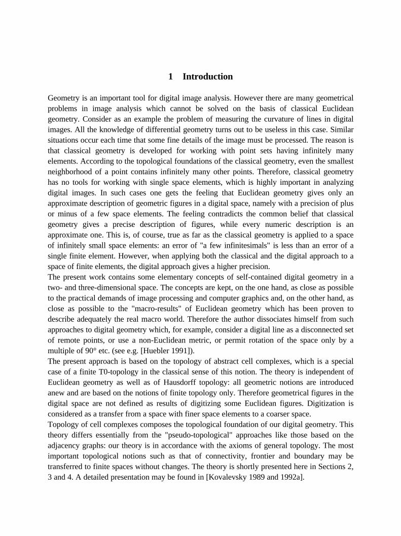
Fig. 1. The surface of a polyhedron considered as a topological space
As an example of a finite topological space consider the surface of a finite polyhedron (Fig. 1).It consists of three kinds of space elements: faces, edges and vertices. An edge l bounds twofaces, say f' and f".
f' l f"
v'
v"
The edge l is bounded by two vertices v' and v". These two vertices are also said to bound thefaces f' and f". Let us declare as open any subset S of faces, edges and vertices, such that forevery element e of S all elements of the surface which are bounded by e are also in S.According to this declaration a face is an open subset. An edge l with the two faces f' and f"bounded by it, also compose an open subset. So does a vertex united with all edges and facesbounded by it. It is easy to see that the open subsets such defined satisfy the axioms. Hence, atopological space is defined. It is finite if the surface of the polyhedron has a finite number ofelements. It is locally finite if each element is bounded by and bounds a finite number of otherelements.
The elements of such a space are not topologically equivalent: for example, a face f' boundedby the edge l, belongs to all open subsets containing l, but l does not belong to the set {f'}which is an open subset containing f'. One can see that this kind of order relation between theelements corresponds to the bounding relation.
Further, it is possible to assign numbers to the space elements in such a way that elements withlower numbers are bounding those with higher numbers. The numbers are called dimensions ofthe space elements. Thus vertices which are not bounded by other elements get the lowestdimension, say 0; the edges get the dimension 1 and the faces the dimension 2. Structures ofthis kind are known as abstract cell complexes [Steinitz 1908].
2.1. Cell complexes
Definition 1: An abstract cell complex C=(E,B,dim) (ACC) is a set E of abstract elementsprovided with an antisymmetric, irreflexive, and transitive binary relation B ⊂ E × E called thebounding relation, and with a dimension function dim: E à I from E into the set I of non-negative integers such that dim(e') < dim(e") for all pairs (e',e")∈B.
Elements of E are called abstract cells. It is important to stress that abstract cells should not beregarded as point sets in a Euclidean space. That is why ACCs and their cells are calledabstract. Considering cells as abstract space elements makes it possible to develop thetopology of ACCs as a self-contained theory which is independent of the topology ofEuclidean spaces.
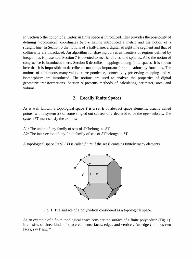
If the dimension dim(e') of a cell e' is equal to d then e' is called a d-dimensional cell or a d-cell. An ACC is called k-dimensional or a k-complex if the dimensions of all its cells are less orequal to k. If (e',e")∈B then e' is said to bound e".Examples of ACCs are shown in Fig. 2. Here and in the sequel the following graphicalnotations (similar to that of Fig. 1) are used: 0-cells are denoted by small circles or squaresrepresenting points, 1-cells are denoted by line segments, 2-cells by interiors of rectangles, 3-cells by interiors of polyhedrons. The bounding relation in these examples is defined in anatural way: a 1-cell represented in the figure by a line segment is bounded by the 0-cellsrepresented by its end points, a 2-cell represented by the interior of a square is bounded by the0- and 1-cells composing its boundary etc.
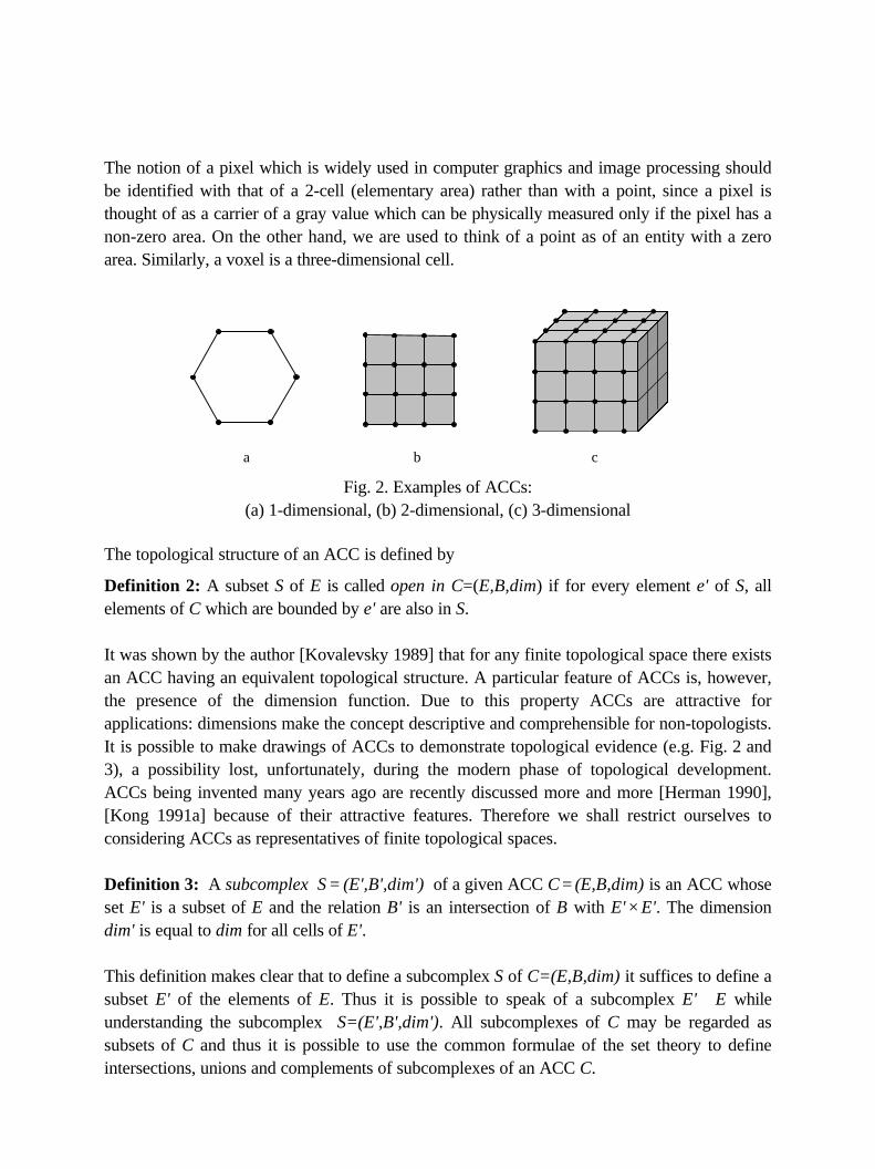
The notion of a pixel which is widely used in computer graphics and image processing shouldbe identified with that of a 2-cell (elementary area) rather than with a point, since a pixel isthought of as a carrier of a gray value which can be physically measured only if the pixel has anon-zero area. On the other hand, we are used to think of a point as of an entity with a zeroarea. Similarly, a voxel is a three-dimensional cell.
a b c
Fig. 2. Examples of ACCs:(a) 1-dimensional, (b) 2-dimensional, (c) 3-dimensional
The topological structure of an ACC is defined by
Definition 2: A subset S of E is called open in C=(E,B,dim) if for every element e' of S, allelements of C which are bounded by e' are also in S.
It was shown by the author [Kovalevsky 1989] that for any finite topological space there existsan ACC having an equivalent topological structure. A particular feature of ACCs is, however,the presence of the dimension function. Due to this property ACCs are attractive forapplications: dimensions make the concept descriptive and comprehensible for non-topologists.It is possible to make drawings of ACCs to demonstrate topological evidence (e.g. Fig. 2 and3), a possibility lost, unfortunately, during the modern phase of topological development.ACCs being invented many years ago are recently discussed more and more [Herman 1990],[Kong 1991a] because of their attractive features. Therefore we shall restrict ourselves toconsidering ACCs as representatives of finite topological spaces.
Definition 3: A subcomplex S = (E',B',dim') of a given ACC C = (E,B,dim) is an ACC whoseset E' is a subset of E and the relation B' is an intersection of B with E' × E'. The dimensiondim' is equal to dim for all cells of E'.
This definition makes clear that to define a subcomplex S of C=(E,B,dim) it suffices to define asubset E' of the elements of E. Thus it is possible to speak of a subcomplex E' ⊂ E whileunderstanding the subcomplex S=(E',B',dim'). All subcomplexes of C may be regarded assubsets of C and thus it is possible to use the common formulae of the set theory to defineintersections, unions and complements of subcomplexes of an ACC C.
Definition 2 of open subsets simultaneously defines the open subcomplexes of a given ACC.
According to the axioms of topology any intersection of a finite number of open subsets is
open. In a finite space there is only a finite number of subsets. Therefore in a finite ACC the
intersection of all open subcomplexes containing a given cell c is an open subcomplex. It is
called the smallest open neighborhood of c in the given ACC C and will be denoted by
SON(c). Notice that there is no such notion at all for a connected Hausdorff space.
2 D 3 D
Cl(c0) SON(c0)
Cl(c1) SON(c1)
Cl(c2) SON(c2)
Cl(c3) ∅ SON(c3)
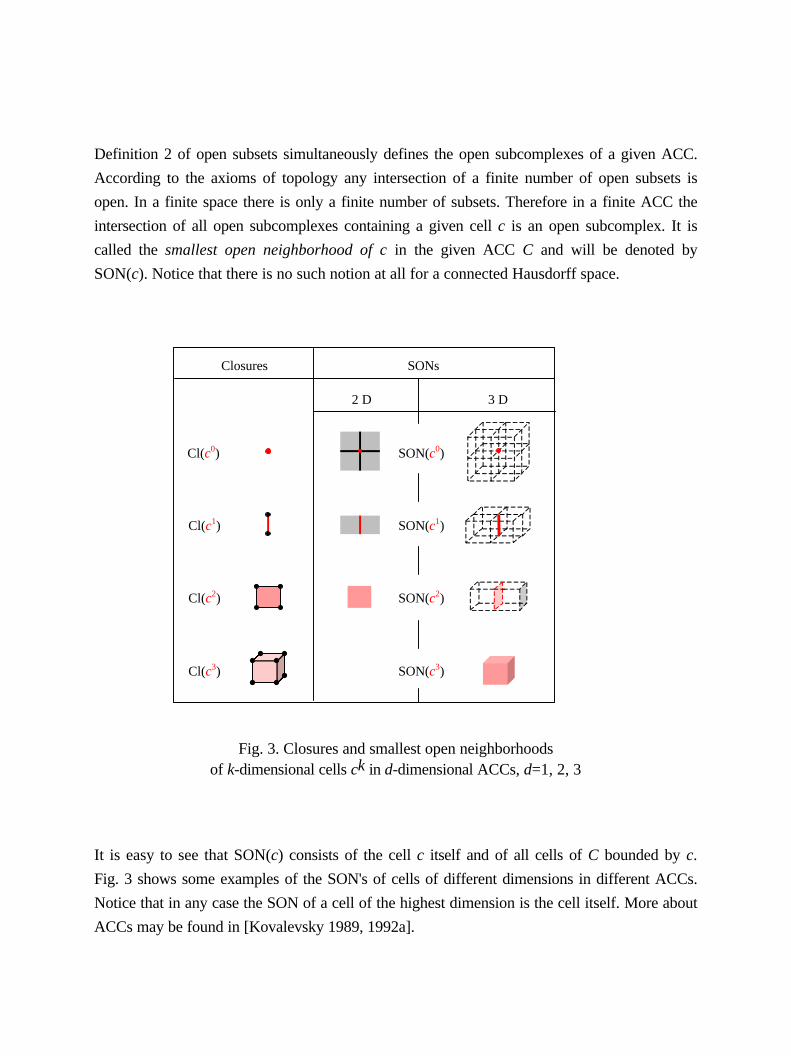
Fig. 3. Closures and smallest open neighborhoodsof k-dimensional cells ck in d-dimensional ACCs, d=1, 2, 3
It is easy to see that SON(c) consists of the cell c itself and of all cells of C bounded by c.
Fig. 3 shows some examples of the SON's of cells of different dimensions in different ACCs.
Notice that in any case the SON of a cell of the highest dimension is the cell itself. More about
ACCs may be found in [Kovalevsky 1989, 1992a].
Closures SONs
2.2. Multidimensional manifolds
There are spaces with some especially simple structure. They are called manifolds. The notionof manifolds in the Hausdorff topology is defined in a rather complex way. In the finitetopology a manifold may be defined in a simple way: a finite manifold is a connectednonbranching finite space. To make this notion more precise let us introduce:
Definition 4: Two cells e' and e" of an ACC C are called incident with each other in C iffeither e'=e", or e' bounds e", or e" bounds e'.
Definition 5: Two ACCs are called B-isomorphic to each other if there exists a one-to-onecorrespondence between their cells which retains the bounding relation.
Definition 6: An n-dimensional finite manifold Mn, n≤3, is an n-dimensional ACC satisfyingthe following conditions:
a) a 0-dimensional manifold M0 consists of two cells with no bounding relation between them;
b) an n-dimensional manifold Mn with n>0 is connected;
c) for any 0-cell c of Mn the subcomplex of all cells different from c and incident with c is B-isomorphic to an (n−1)-dimensional sphere (nonbranching condition).
This definition corresponds to the well-known definition of a combinatorial manifold.
Topological properties of two-dimensional manifolds are well known. They are defined by thegenus which in turn is defined by the Euler polyhedron formula:
N2 − N1 + N0 = 2⋅(1−G).
Here N2, N1 and N0 are the numbers of 2-, 1- and 0-dimensional cells correspondingly, G is thegenus.
The notion of the genus can be illustrated by the following remarks: a manifold of genus 0looks like a sphere (subdivided into cells), a manifold of genus 1 looks like a torus. A manifoldof genus equal to G looks like a sphere with G handles.
Properties of manifolds of higher dimensions are still not sufficiently investigated. On the otherhand, they may be of great interest for our understanding of the universe since there arereasons to believe that our physical space-time is a four-dimensional manifold. Topologicalproperties of the space may be of great importance for the theory of elementary particles. SinceACCs of any dimension may be easily represented in computers there is a possibility ofinvestigating the properties of finite manifolds of dimensions greater than two by means ofcomputers.
3 Connectivity
Consider now the transitive closure of the incidence relation according to Definition 4. (Thetransitive closure of a binary relation R in E is the intersection of all transitive relations in Econtaining R). This new relation will be declared as the connectedness relation. As anytransitive closure it may be defined recursively:
Definition 7: Two cells e' and e" of an ACC C are called connected to each other in C iffeither e' is incident with e", or there exists in C a cell c which is connected to both e' and e".
It may be easily shown that the connectedness relation according to Definition 7 is anequivalence relation (reflexive, symmetric and transitive). Thus it defines a partition of an ACCC into equivalence classes called the components of C.
Definition 8: An ACC C consisting of a single component is called connected.
It is easy to see that Definitions 7 and 8 are directly applicable to subsets of an ACC C: anysubset is according to Definition 3 a subcomplex of C and is again an ACC. It is, however,important to stress that all intermediate cells c mentioned in Definition 7 must belong to thesubset under consideration. Therefore it is reasonable to regard an equivalent definition ofconnected ACCs:
Definition 9: A sequence of cells of an ACC C beginning with c' and finishing with c" is calleda path in C from c' to c" if every two cells which are adjacent in the sequence are incident.
Definition 10: An ACC C is called path-connected if for any two cells c' and c" of C thereexists a path in C from c' to c" .
Kong et al. [Kong 1991b] have shown that Definitions 8 and 10 are equivalent. As shown bythe author [Kovalevsky 1989, 1992a] these definitions are in full accordance with classicaltopology and free of paradoxes.
3.1. Membership rules
An n-dimensional image (n=2 or 3) is defined by assigning numbers (gray values or densities)
to the n-dimensional cells of an n-dimensional ACC. There is no need to assign gray values or
densities to cells of lower dimensions. Such an assignment would be unnatural since a gray
value may be physically determined only for a finite area. We have agreed to interpret 2-cells in
a two-dimensional ACC as elementary areas. Cells of lower dimensions have area equal to
zero. Similarly, a density may be physically determined only for a finite volume which is
represented in a three-dimensional ACC by a 3-cell.
However, when considering the connectivity of a subset (subcomplex) of an n-dimensional
ACC, the membership in a subset under consideration must be specified for cells of all
dimensions. Under this condition the connectivity of the subset is consistently specified by
Definition 8 or 10. It is important to stress that the connectivity is determined by means of the
lower dimensional cells which are serving as some kind of "glue" joining n-dimensional cells. A
set consisting of only n-dimensional cells is always disconnected.
Generally a partition of the ACC in disjoint subsets must be given and each cell of the ACC
must be assigned to exactly one subset of the partition. If an ACC and its subcomplexes under
consideration are given then every cell has the identification number of a subcomplex as its
membership label. If, however, only the set of the n-dimensional cell with their gray values, or
densities, and/or membership labels is given (which is often the case in image processing) then
the membership of cells of lower dimensions cannot be specified in the same way as that of the
cells of highest dimension (n-cells) since the lower dimensional cells have no gray values. This
must be done by using certain a priori knowledge about the image under consideration. The
membership of a lower dimensional cell may be specified as a function of the membership
labels and of the gray levels (densities) of the n-cells bounded by it by means of the
membership rules. Consider an examples of such a rule.
Maximum Value Rule: In an n-dimensional ACC every cell c of dimension less than n gets
the membership label of that n-cell which has the maximum gray value (density) among all n-
cells bounded by c.
It is possible to formulate a similar Minimum Value Rule. The connectivity of a binary image is
similar in both cases to that obtained according to a widely used idea of an 8-adjacency for
objects and a 4-adjacency for the background [Rosenfeld 1976]. An important advantage of
the Maximum (Minimum) Value Rule is the possibility of using it for many-valued images. A
slightly more complicated and also practically useful rule may be found in [Kovalevsky 1989].
Also situations in which an explicit specification of the membership labels may be useful, are
discussed there.
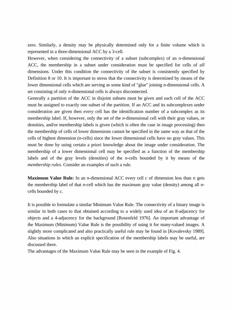
The advantages of the Maximum Value Rule may be seen in the example of Fig. 4.
The image has three gray values: 8 (dark gray in Fig. 4), 1 (light gray) and 0 (white). When
applying the Maximum Value Rule, then the 0-cells shown as dark circles obtain their
membership from the pixels with the gray value 8, the 0-cells shown as light circles belong to
the sets with the gray level 1. The remaining 0-cells belong to the set with the gray level 0.
Correspondingly, the image has 2 components with the value 8; 3 components with the value
1; and 5 components with the value 0. This is in accordance with our intuitive idea of
connected components.
Fig. 4. An image with three gray values
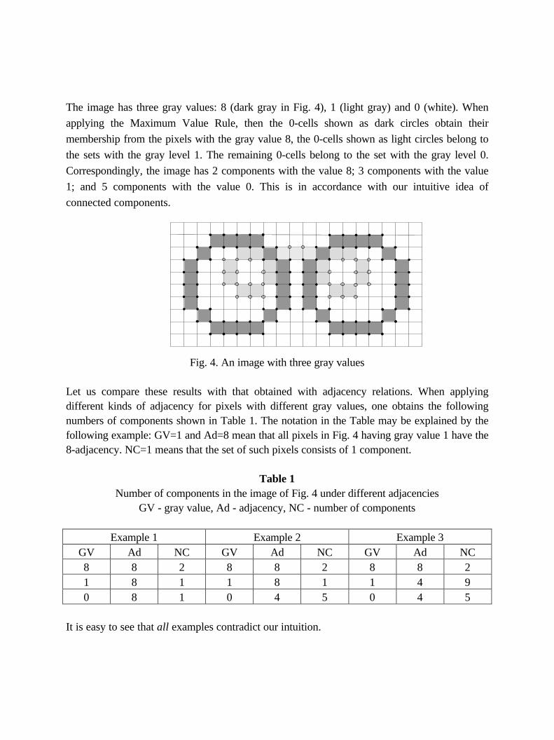
Let us compare these results with that obtained with adjacency relations. When applyingdifferent kinds of adjacency for pixels with different gray values, one obtains the followingnumbers of components shown in Table 1. The notation in the Table may be explained by thefollowing example: GV=1 and Ad=8 mean that all pixels in Fig. 4 having gray value 1 have the8-adjacency. NC=1 means that the set of such pixels consists of 1 component.
Table 1Number of components in the image of Fig. 4 under different adjacencies
GV - gray value, Ad - adjacency, NC - number of components
Example 1 Example 2 Example 3GV Ad NC GV Ad NC GV Ad NC8 8 2 8 8 2 8 8 21 8 1 1 8 1 1 4 90 8 1 0 4 5 0 4 5
It is easy to see that all examples contradict our intuition.
3.2. Labelling and counting connected components
Definition 7 may be directly used to label connected components of a segmented image. Givenis a digital image as a two- or three-dimensional array with gray values (densities) assigned toeach pixel (voxel). Results of the segmentation of the image into quasi-homogeneous segmentsare also given as segment labels assigned to each pixel (voxel).The problem of labeling connected components consists in assigning to each pixel (voxel) ofthe image the identification number of the component to which it belongs.
The well-known solution for two-dimensional binary images [Rosenfeld 1976] is as follows.The image is scanned row by row. For each pixel P the following set S(P) of pixels is defined:a pixel belongs to S(P) if it is adjacent to P, is already visited, and has the same segmentationlabel as P. If S(P) is empty, then P gets a new component number. If all components of S(P)have the same component number, then P gets this number. If S(P) consists of more than onecomponent and the components of S(P) have different component numbers, then P gets one ofthe numbers and all the numbers are recorded as being equivalent. When the image iscompletely scanned in this way, the records must be investigated and the classes of equivalentnumbers determined. The image must then be rescanned and the old numbers must be replacedby the numbers of equivalence classes.The algorithm based on ACCs [Kovalevsky 2000] is similar to that just described. The maindifference consists in the following. The set S(P) of adjacent pixels is replaced by the set C(P)of cells of lower dimensions incident with P, which are simultaneously incident to some alreadyvisited pixels. Each cell of C(P) gets its segment label according to a membership rule asexplained in the previous section. The cell gets also the corresponding component numberfrom one of the already visited pixels. Now the subset C'(P)⊂C(P) having the samesegmentation label as P is investigated in the same way as the set S(P). The advantage of thisprocedure is that it may be used for non-binary images while avoiding wrong decisionsdemonstrated in Table 1.Unfortunately, in most publications (including [Rosenfeld 1976]) there is no description of anefficient procedure for finding the equivalence classes. The few procedures described in theliterature need either much computation time or an additional memory space greater than theoutput image containing the component labels. Our component labeling algorithm [Kovalevsky2001] finds the equivalence classes without any additional memory. The processing time istwice the time of scanning the image.
The problem of counting the components is much simpler than that of labeling them since noequivalence classes need to be determined. The subset C'(P) must be determined in the sameway as before. The component counter is first incremented by 1 for each pixel P. Then thecounter must be decremented by the number of components of C'(P).
4 Boundaries and frontiers
The theory of ACCs leads to topologically consistent definitions of the boundary and thefrontier of a subset of an image. The notion of a frontier remains the same as in generaltopology:
Definition 11a: The frontier of a subcomplex S of an ACC C relative to C is the subcomplexFr(S,C) consisting of all cells c of C such that the SON(c) contains cells both of S and of itscomplement C-S.
Definition 11b: The boundary ∂Ck of an k-dimensional ACC Ck is the closure of the set of all(k−1)-dimensional cells each of which bounds exactly one k-dimensional cell of Ck.
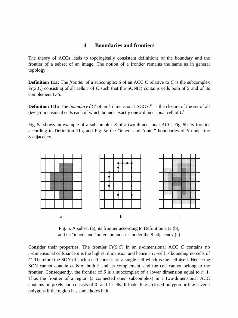
Fig. 5a shows an example of a subcomplex S of a two-dimensional ACC, Fig. 5b its frontieraccording to Definition 11a, and Fig. 5c the "inner" and "outer" boundaries of S under the8-adjacency.
a b c
Fig. 5. A subset (a), its frontier according to Definition 11a (b),and its "inner" and "outer" boundaries under the 8-adjacency (c)
Consider their properties. The frontier Fr(S,C) in an n-dimensional ACC C contains non-dimensional cells since n is the highest dimension and hence an n-cell is bounding no cells ofC. Therefore the SON of such a cell consists of a single cell which is the cell itself. Hence theSON cannot contain cells of both S and its complement, and the cell cannot belong to thefrontier. Consequently, the frontier of S is a subcomplex of a lower dimension equal to n−1.Thus the frontier of a region (a connected open subcomplex) in a two-dimensional ACCcontains no pixels and consists of 0- and 1-cells. It looks like a closed polygon or like severalpolygons if the region has some holes in it.
The frontiers according to Definition 11a are analogous to the "(C,D)-borders" or sets of"cracks" briefly mentioned in [Rosenfeld 1976, second edition]. Similarly, the frontier of aregion in a three-dimensional ACC contains no voxels and consists of 0-, 1-, and 2-cells. Itlooks like a closed surface of a polyhedron (or several surfaces if the region has some cavities).A 2-cell of a frontier separates a voxel of the region from a voxel of its complement. Thus the2-cells of the frontier are the "faces" considered in [Herman 1983]. We may see now that thetheory of the ACCs brings many intuitively introduced notions together in a consistent andtopologically well founded concept.The frontiers Fr(S,C) in two-dimensional images have a zero area and frontiers in three-dimensional images a zero volume, which is not the case for boundaries in adjacency graphs(see Fig. 5c).The next peculiarity of the frontier Fr(S,C) is that it is unique: there is no need (and nopossibility!) of distinguishing between the inner and outer boundary as they were defined, forexample, by Pavlidis [Pavlidis 1977] or between the "D-border of C" and "C-Border of D"[Rosenfeld 1976]. A boundary according to Definition 11a is one and the same for a subset andfor its complement, since Definition 11a is symmetric with respect to both subsets. This is notthe case for boundaries in adjacency graphs.The frontier Fr(S,C) depends neither on the kind of adjacency (which notion is no more used)nor on the membership rules as defined in Section 3. The proof of the last assertion may befound in [Kovalevsky 1992a].Algorithms for tracking frontiers are important for applications. When using the concept ofACCs the algorithms become simpler and more comprehensible. Such an algorithm for two-dimensional spaces is described in [Kovalevsky 1992a] and for three-dimensional spaces in[Kovalevsky 1999]. Similarly, algorithms for filling interiors of closed curves are simpler whenusing ACCs. Such an algorithm is presented in [Kovalevsky 1992a].
5 Locally finite Cartesian spaces
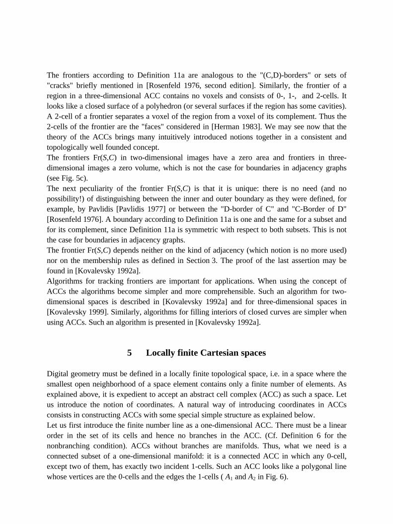
Digital geometry must be defined in a locally finite topological space, i.e. in a space where thesmallest open neighborhood of a space element contains only a finite number of elements. Asexplained above, it is expedient to accept an abstract cell complex (ACC) as such a space. Letus introduce the notion of coordinates. A natural way of introducing coordinates in ACCsconsists in constructing ACCs with some special simple structure as explained below.Let us first introduce the finite number line as a one-dimensional ACC. There must be a linearorder in the set of its cells and hence no branches in the ACC. (Cf. Definition 6 for thenonbranching condition). ACCs without branches are manifolds. Thus, what we need is aconnected subset of a one-dimensional manifold: it is a connected ACC in which any 0-cell,except two of them, has exactly two incident 1-cells. Such an ACC looks like a polygonal linewhose vertices are the 0-cells and the edges the 1-cells ( A1 and A2 in Fig. 6).
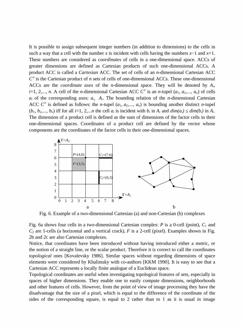
It is possible to assign subsequent integer numbers (in addition to dimensions) to the cells insuch a way that a cell with the number x is incident with cells having the numbers x−1 and x+1.These numbers are considered as coordinates of cells in a one-dimensional space. ACCs ofgreater dimensions are defined as Cartesian products of such one-dimensional ACCs. Aproduct ACC is called a Cartesian ACC. The set of cells of an n-dimensional Cartesian ACCC n is the Cartesian product of n sets of cells of one-dimensional ACCs. These one-dimensionalACCs are the coordinate axes of the n-dimensional space. They will be denoted by Ai,i=1, 2,..., n. A cell of the n-dimensional Cartesian ACC C n is an n-tupel (a1, a2,..., an) of cellsai of the corresponding axes: ai∈ Ai. The bounding relation of the n-dimensional CartesianACC C n is defined as follows: the n-tupel (a1, a2,..., an) is bounding another distinct n-tupel(b1, b2,..., bn) iff for all i=1, 2,...n the cell ai is incident with bi in Ai and dim(ai) ≤ dim(bi) in Ai.The dimension of a product cell is defined as the sum of dimensions of the factor cells in theirone-dimensional spaces. Coordinates of a product cell are defined by the vector whosecomponents are the coordinates of the factor cells in their one-dimensional spaces.
a bFig. 6. Example of a two-dimensional Cartesian (a) and non-Cartesian (b) complexes
Fig. 6a shows four cells in a two-dimensional Cartesian complex: P is a 0-cell (point), C1 andC2 are 1-cells (a horizontal and a vertical crack), F is a 2-cell (pixel). Examples shown in Fig.2b and 2c are also Cartesian complexes.Notice, that coordinates have been introduced without having introduced either a metric, orthe notion of a straight line, or the scalar product. Therefore it is correct to call the coordinatestopological ones [Kovalevsky 1986]. Similar spaces without regarding dimensions of spaceelements were considered by Khalimsky with co-authors [KKM 1990]. It is easy to see that aCartesian ACC represents a locally finite analogue of a Euclidean space.Topological coordinates are useful when investigating topological features of sets, especially inspaces of higher dimensions. They enable one to easily compute dimensions, neighborhoodsand other features of cells. However, from the point of view of image processing they have thedisadvantage that the size of a pixel, which is equal to the difference of the coordinate of thesides of the corresponding square, is equal to 2 rather than to 1 as it is usual in image
F=(3,5)
C1=(7,6)
C2=(6,3)
P=(4,6)
0 1 2 3 4 5 6 7 8
8
7
6
5
4
3
2
1
0
Y=A2
X=A1
processing. There are two possibilities to overcome this drawback. One of them consists inassigning to a 0-cell and to the next incident 1-cell of an axis the same integer number.Dimensions of cells must then be coded by additional labels. This notation gives no possibilityof expressing the fine difference in the location of a pixel and of one of the 0-cells incident withit. This leads sometimes to an undesired asymmetry of figures described by inequalities. Forexample, a digital circle defined as a set of pixels whose distance to a point, i.e. to a 0-cell, islimited by the given radius is asymmetric with respect to the point.The second possibility is to assign subsequent rational numbers with denominator 2 tosubsequent cells of an axis. The size of a pixel is then equal to 1 and cells of differentdimensions have always different coordinates. Under this notation the coordinates of a pixel ina two-dimensional space and, generally, of an n-cell c in an n-dimensional space, are equal tothe arithmetic mean of the coordinates of all cells bounding c. Hence, fractional coordinates ofan n-cell may be interpreted as coordinates of its "middle point". This prevents the imprecisedefinition of figures by inequalities. In the general case coordinates may be rational numberswith any constant denominator, or floating point numbers while an even mantissa correspondsto a 0-cell and an odd mantissa to a 1-cell. It is possible to achieve under such a notation anywanted precision of determining the coordinates while preserving the possibility to recognizethe dimension of a cell from its coordinates. Let us consider in the sequel coordinates of cellsof the axes as rational numbers with denominator 2. Then dimensions of cells may berecognized in the following way: the coordinates of 0-cells of the axes are integers and that of1-cells are fractions. All n coordinates of a 0-cell of C n are integers. All coordinates of ann-cell are fractions. A d-dimensional cell of C n has d fractional and n−d integer coordinates.The recognition of dimensions in the general case of an arbitrary denominator is similar to thatjust explained.
6 Linear inequalities in a two-dimensional space
To make the reading easier, let us call the 0-cells of the space "points", the 1-cells "cracks" andthe 2-cells "pixels". Let us introduce some definitions, important for the future.
Definition 12: A region is an open connected subset of the space. A region R of an n-dimensional ACC C n is called solid if every cell c∈C n which is not in R is incident with an n-cell of the complement C n−R.
Definition 13: A digital half-plane is a solid region containing all pixels of the space, whosecoordinates satisfy a linear inequality.
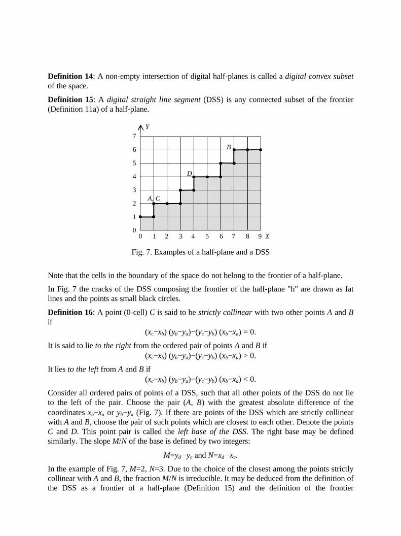
For example, Fig. 7 shows the half-plane defined by 2x−3y+2 > 0. All pixels of the half-plane inFig. 7 are shaded.
Definition 14: A non-empty intersection of digital half-planes is called a digital convex subsetof the space.
Definition 15: A digital straight line segment (DSS) is any connected subset of the frontier(Definition 11a) of a half-plane.
Fig. 7. Examples of a half-plane and a DSS
Note that the cells in the boundary of the space do not belong to the frontier of a half-plane.
In Fig. 7 the cracks of the DSS composing the frontier of the half-plane "h" are drawn as fatlines and the points as small black circles.
Definition 16: A point (0-cell) C is said to be strictly collinear with two other points A and Bif
(xc−xb)⋅(yb−ya)−(yc−yb)⋅(xb−xa) = 0.
It is said to lie to the right from the ordered pair of points A and B if(xc−xb)⋅(yb−ya)−(yc−yb)⋅(xb−xa) > 0.
It lies to the left from A and B if(xc−xb)⋅(yb−ya)−(yc−yb)⋅(xb−xa) < 0.
Consider all ordered pairs of points of a DSS, such that all other points of the DSS do not lieto the left of the pair. Choose the pair (A, B) with the greatest absolute difference of thecoordinates xb−xa or yb−ya (Fig. 7). If there are points of the DSS which are strictly collinearwith A and B, choose the pair of such points which are closest to each other. Denote the pointsC and D. This point pair is called the left base of the DSS. The right base may be definedsimilarly. The slope M/N of the base is defined by two integers:
M=yd −yc and N=xd −xc.
In the example of Fig. 7, M=2, N=3. Due to the choice of the closest among the points strictlycollinear with A and B, the fraction M/N is irreducible. It may be deduced from the definition ofthe DSS as a frontier of a half-plane (Definition 15) and the definition of the frontier
7
6
5
4
3
2
1
00 1 2 3 4 5 6 7 8 9 X
A, C
D
B
Y
(Definition 11a) that every point (x, y) of the DSS satisfies the following inequalities:
0 ≤ (x−xc)⋅M−(y−yc)⋅N ≤ M + N −1. (1)
Note that x, y, xc, yc, M and N are all integers. This inequalities are used for the fastrecognition of DSSs [Kovalevsky 1990, 1997].
Definition 17: A two-dimensional vector with integer components (x, y) is called right semi-collinear with another integer vector (n, m) if the following inequalities hold:
0 ≤ (x⋅M − y⋅N) ≤ M + N −1
where M and N are numerator and denominator of the irreducible fraction M/N = m/n.
The notion of left semi-collinear vectors may be defined similarly.
By means of this definition, a DSS with a given base (C, D) may be defined as such a digitalcurve K (connected subset of a one-dimensional manifold, see Definition 6) that each point Pof K composes with one of the end points of the right base (say, C) a vector (P−C) left semi-collinear with the vector (D−C) of the right base. A similar definition is possible when usingthe left base.
One of the simplest methods to draw a DSS in a two-dimensional ACC consists in tracking thelinear inequality defining the corresponding half-plane. For this purpose the tracking algorithmdescribed in [Kovalevsky 1992a] may be used. To adapt the algorithm for tracking aninequality rather than an object in a binary image, the tests of the two pixels L and R as to theirmembership in the object must be replaced by the test, whether the half-integer coordinates ofthe pixels satisfy the inequality. The tracking may be made faster when calculating theincrements of the left side of the inequality rather than the expression itself. The calculationbecomes still simpler when transforming the desired DSS to one lying in the first octant. Thismodification of the tracking corresponds to the famous Bresenham algorithm [Bresenham1965].
The tracking technique may be used to draw frontiers of regions defined by any inequalities,also non-linear, e.g. circles, parabolas etc.
7 Metric, circles and spheres
No other metric but the Euclidean must be used in digital geometry. This is necessary to obtainresults as close as possible to those of classical geometry. Correspondingly, the distanceD(A,B) between two points (cells) A and B is declared to be equal to
2
1
)(),( ii
n
i
BABAD −= ∑=
Ai and Bi being the ith coordinates of the corresponding points in an n-dimensional Cartesianspace as defined in Section 5.
Having defined the distance, we may immediately specify the inequality of a digital disk in thetwo-dimensional space:
Definition 18: A digital disk is a solid region containing all pixels of the space, whosecoordinates satisfy the following inequality:
(x−xc)2 + (y−yc)
2 < R2 ; (2)
where x and y are the half-integer coordinates of pixels, xc and yc are the coordinates of thecenter, R is the radius of the disk. The values of xc, yc and R may be either integer or fractional.
Definition 19: A digital circular arc (DCA) is any connected subset of the frontier of a digitaldisk.
To draw a DCA, the technique of tracking the frontier of an inequality, as described in theprevious section, may be used. As in the case of a line, the tracking may be made faster whencalculating the increments of the left side of (2) rather than the expression itself and whenrestricting the set of possible step directions according to the known octant of the arc. Thismodification of tracking is well-known in computer graphics as the Bresenham arc algorithm[Bresenham 1977]. The recognition of DCAs is described by the author in [Kovalevsky 1990].
In a similar way digital balls and spheres (as boundaries of balls) may be defined in the three-dimensional space. Tracking surfaces in three-dimensional binary images is described in[Kovalevsky 1999]. The same technique may be used to track the surface of an arbitrary bodydefined by an inequality.
The notions of distance and collinearity may be used to introduce that of congruence:
Definition 20: The distances d between two points is declared digitally equal to a number n, ifthe absolute difference between d and n is less or equal to the length of a pixel's diagonal (√2under the accepted notation).
Definition 21: The value of semi-collinearity of a point C relative to an ordered pair of pointsA and B is declared to be 0 if C is semi-collinear with (A, B). If it is not semi-collinear, then thevalue is declared to be −1 or +1 depending on whether C lies to the left or to the right of (A, B)according to Definition 16.
Definition 22: Two figures F and G are called congruent with each other iff there exists such amapping from F to G that the distance between any two cells of G is digitally equal to thedistance of their preimages in F and the value of semi-collinearity of any three points of G isthe same as of their preimages in F.
The mapping is not necessarily a bijection. The class of considerable mappings called CPM isdescribed in the next section.
8 Mappings among locally finite spaces
Mappings among locally finite spaces are rather different from those among Hausdorff spaces.Consider the simplest example of mapping a one-dimensional finite space X onto another suchspace Y by a function. A function must assign one cell of Y to each cell of X. Consider afunction F and a subset S of Y consisting of two incident cells (Definition 4) of Y having thecoordinates y and y+1/2. The preimage F −1(S) must consist of at least two different cells, sincethe function is single-valued. The difference Dy between the values of y is equal to 1/2, whilethe difference Dx between the extreme values of x in F −1(S) is greater or equal to 1/2. Hencethe average slope Dy /Dx of F cannot be greater than 1. Thus a problem arises: functionsmapping one locally finite one-dimensional space into another such space cannot have a slopegreater than 1. If we decide to restrict ourselves to such functions, another problem arises:there is no possibility of considering inverse functions, which in this case must have a slopegreater than or equal to 1. The only possible solution is to consider more generalcorrespondences between X and Y, assigning to each cell of X a subset of Y rather than a singlecell.
8.1. Connectivity-preserving correspondences
A correspondence between X and Y or a many-valued mapping of X into Y is a subset F ofordered pairs (x, y) containing all cells x∈X and some cells y∈Y. There is a difference betweena correspondence and a binary relation: in the case of a relation the sets X and Y must beidentical. A function is a special case of a correspondence: a correspondence is a function ifany value of x∈X is encountered in exactly one pair (x, y) of F. Given a correspondence F, theset of all y encountered in pairs of F containing a fixed x is called the image of x. The set of allx encountered in pairs of F with a fixed y is called the preimage of y. The union of the imagesof all x of a subset SX of X is called the image of SX. Similarly, the union of the preimages ofall y of a subset SY of Y is called the preimage of SY. A correspondence may be continuous inthe classical sense of the notion if the preimage of any open subset of Y is open (e.g. G in Fig.8; coordinates in Fig. 8 are denoted by their numerators, to make the notation simpler).However, in digital geometry another class of correspondence is important.
Definition 23: A correspondence between X and Y is called a connectivity preserving mapping(CPM) if the image of any connected subset of X is connected.
An example of a CPM is the correspondence F in Fig. 8. It is easy to see that every continuouscorrespondence is a CPM but not vice versa.
Let us denote by V(x,y) the connected component of F(x) containing y and by H(x,y) theconnected component of F −1(y) containing x.
Definition 24: A correspondence F is called simple if for each pair (x, y)∈F at most one of thesets V(x,y) and H(x,y) contains more than one element.
For example, the correspondence F in Fig. 8 is a simple CPM, while the correspondence G isnot simple since for the pair x=13, y=3 both V(x,y) and H(x,y) contain more than one cell. We
shall consider in what follows mainly simple CPM's which are substitutes of continuousmappings in locally finite spaces.
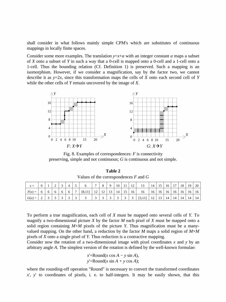
Consider some more examples. The translation y=x+a with an integer constant a maps a subsetof X onto a subset of Y in such a way that a 0-cell is mapped onto a 0-cell and a 1-cell onto a1-cell. Thus the bounding relation (Cf. Definition 1) is preserved. Such a mapping is anisomorphism. However, if we consider a magnification, say by the factor two, we cannotdescribe it as y=2x, since this transformation maps the cells of X onto each second cell of Ywhile the other cells of Y remain uncovered by the image of X.
F: XàY G: XàY
Fig. 8. Examples of correspondences: F is connectivitypreserving, simple and not continuous; G is continuous and not simple.
Table 2Values of the correspondences F and G
x = 0 1 2 3 4 5 6 7 8 9 10 11 12 13 14 15 16 17 18 19 20
F(x) = 6 6 6 6 6 7 [8,11] 12 12 13 14 15 16 16 16 16 16 16 16 16 16
G(x) = 2 3 3 3 3 3 3 3 3 3 3 3 3 [3,11] 12 13 14 14 14 14 14
To perform a true magnification, each cell of X must be mapped onto several cells of Y. Tomagnify a two-dimensional picture X by the factor M each pixel of X must be mapped onto asolid region containing M×M pixels of the picture Y. Thus magnification must be a many-valued mapping. On the other hand, a reduction by the factor M maps a solid region of M×Mpixels of X onto a single pixel of Y. Thus reduction is a contractive mapping.Consider now the rotation of a two-dimensional image with pixel coordinates x and y by anarbitrary angle A. The simplest version of the rotation is defined by the well-known formulae:
x'=Round(x⋅cos A − y⋅sin A),y'=Round(x⋅sin A + y⋅cos A);
where the rounding-off operation "Round" is necessary to convert the transformed coordinatesx', y' to coordinates of pixels, i. e. to half-integers. It may be easily shown, that this
0 2 4 6 8 10 15 20
16
12
8
4
0 X
Y
16
12
8
4
00 2 4 6 8 10 15 20
X
Y
transformation maps some pairs of adjacent pixels of the input image onto a single pixel of theoutput. Thus it is a contractive mapping. When using the more perfect "antialiasing" rotation, agray value of an output pixel is calculated as a function of the gray values of four adjacentinput pixels. Such a rotation must be considered as a mapping which is simultaneouslycontractive and many-valued. In any case it is not an isomorphism. However, it isapproximately an isomorphism. Let us give this assertion a precise meaning.
8.2. The notion of n-isomorphism
We have presented in Section 2.1 the notion of the smallest open neighborhood (SON) of a
cell in an ACC. Let us introduce now two more notions which we need to define the n-
isomorphism.
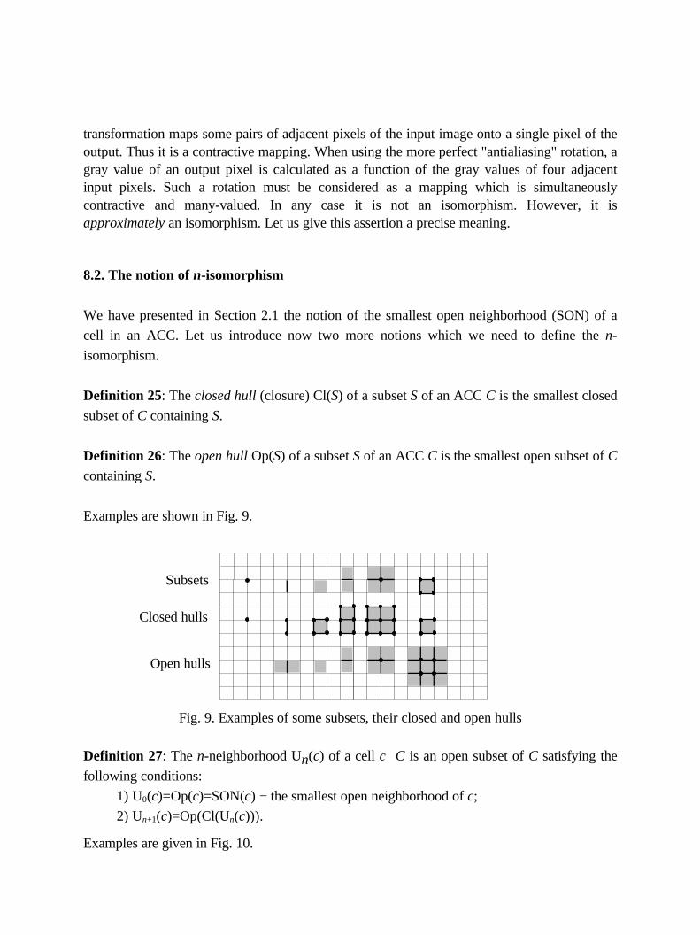
Definition 25: The closed hull (closure) Cl(S) of a subset S of an ACC C is the smallest closed
subset of C containing S.
Definition 26: The open hull Op(S) of a subset S of an ACC C is the smallest open subset of C
containing S.
Examples are shown in Fig. 9.
Subsets
Closed hulls
Open hulls
Fig. 9. Examples of some subsets, their closed and open hulls
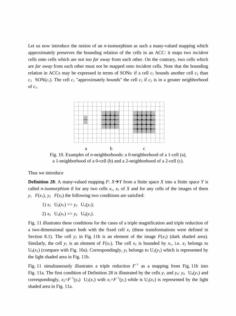
Definition 27: The n-neighborhood Un(c) of a cell c∈C is an open subset of C satisfying the
following conditions:
1) U0(c)=Op(c)=SON(c) − the smallest open neighborhood of c;
2) Un+1(c)=Op(Cl(Un(c))).
Examples are given in Fig. 10.
Let us now introduce the notion of an n-isomorphism as such a many-valued mapping which
approximately preserves the bounding relation of the cells in an ACC: it maps two incident
cells onto cells which are not too far away from each other. On the contrary, two cells which
are far away from each other must not be mapped onto incident cells. Note that the bounding
relation in ACCs may be expressed in terms of SONs: if a cell c1 bounds another cell c2 than
c2∈SON(c1). The cell c1 "approximately bounds" the cell c2 if c2 is in a greater neighborhood
of c1.
a b cFig. 10. Examples of n-neighborhoods: a 0-neighborhood of a 1-cell (a),
a 1-neighborhood of a 0-cell (b) and a 2-neighborhood of a 2-cell (c).
Thus we introduce
Definition 28: A many-valued mapping F: XàY from a finite space X into a finite space Y is
called n-isomorphism if for any two cells x1, x2 of X and for any cells of the images of them
y1∈F(x1), y2∈F(x2) the following two conditions are satisfied:
1) x2∈U0(x1) => y2∈Un(y1);
2) x2∉Un(x1) => y2∉U0(y1).
Fig. 11 illustrates these conditions for the cases of a triple magnification and triple reduction of
a two-dimensional space both with the fixed cell x1 (these transformations were defined in
Section 8.1). The cell y2 in Fig. 11b is an element of the image F(x2) (dark shaded area).
Similarly, the cell y1 is an element of F(x1). The cell x2 is bounded by x1, i.e. x2 belongs to
U0(x1) (compare with Fig. 10a). Correspondingly, y2 belongs to U2(y1) which is represented by
the light shaded area in Fig. 11b.
Fig. 11 simultaneously illustrates a triple reduction F−1 as a mapping from Fig. 11b into
Fig. 11a. The first condition of Definition 28 is illustrated by the cells y1 and y4: y4∈U0(y1) and
correspondingly, x2=F−1(y4)∈U2(x1) with x1=F−1(y1) while is U2(x1) is represented by the light
shaded area in Fig. 11a.
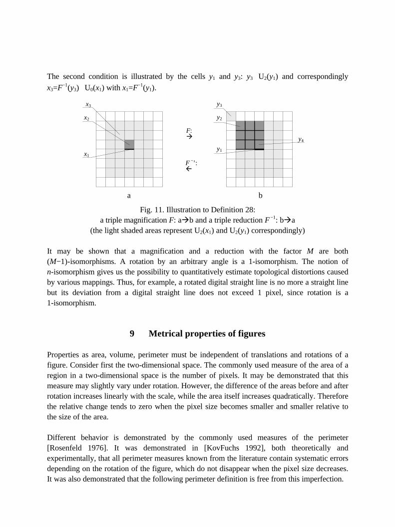
The second condition is illustrated by the cells y1 and y3: y3∉U2(y1) and correspondingly
x3=F−1(y3)∉U0(x1) with x1=F−1(y1).
a b
Fig. 11. Illustration to Definition 28:a triple magnification F: aàb and a triple reduction F −1: bàa
(the light shaded areas represent U2(x1) and U2(y1) correspondingly)
It may be shown that a magnification and a reduction with the factor M are both(M−1)-isomorphisms. A rotation by an arbitrary angle is a 1-isomorphism. The notion ofn-isomorphism gives us the possibility to quantitatively estimate topological distortions causedby various mappings. Thus, for example, a rotated digital straight line is no more a straight linebut its deviation from a digital straight line does not exceed 1 pixel, since rotation is a1-isomorphism.
9 Metrical properties of figures
Properties as area, volume, perimeter must be independent of translations and rotations of afigure. Consider first the two-dimensional space. The commonly used measure of the area of aregion in a two-dimensional space is the number of pixels. It may be demonstrated that thismeasure may slightly vary under rotation. However, the difference of the areas before and afterrotation increases linearly with the scale, while the area itself increases quadratically. Thereforethe relative change tends to zero when the pixel size becomes smaller and smaller relative tothe size of the area.
Different behavior is demonstrated by the commonly used measures of the perimeter[Rosenfeld 1976]. It was demonstrated in [KovFuchs 1992], both theoretically andexperimentally, that all perimeter measures known from the literature contain systematic errorsdepending on the rotation of the figure, which do not disappear when the pixel size decreases.It was also demonstrated that the following perimeter definition is free from this imperfection.
y4
y3
y2
y1
x3
x2
x1
F:à
F −1:ß
Definition 29: The perimeter of a region R in a two-dimensional finite space is the sum of thelengths of subsequent DSSs obtained by subdividing the frontier of R into as few as possibleDSSs.
It was shown in [KovFuchs 1992] that this perimeter estimate is invariant with respect torotation: the absolute difference between the perimeters before and after rotation by anarbitrary angle tends to zero when the size of the pixels (relative to the diameter of the region)decreases.In a three-dimensional finite space the perimeter of a closed digital curve, may be defined inthe same way. Estimation of the area of a two-dimensional surface in a three-dimensional spaceis a problem still more difficult than that of the perimeter. The author supposes that a surfacemust be dissolved into maximum patches of digital planes and the areas of the patches must beadded. However, defining the area of a subset of a plane in the three-dimensional space is itselfa non-trivial problem. The area must be by no means determined as the number of facets (2-cells) in the subset. Such an estimate would have the same imperfection as the perimeterestimate by the number of cracks in a two-dimensional space: the estimate would not berotation invariant. The area of a plane patch in space must be determined as the area of a planepolygon by means of the coordinates of its vertices. The coordinates must be determined bymeans of a procedure for recognizing digital plane patches in space, similar to the recognitionof the DSSs. Unfortunately, no such algorithm is familiar to the author as yet.On the other hand, the estimate of the volume of a three-dimensional region in a three-dimensional space as the number of voxels in the region is supposed to be rotation invariant:the error tends to zero as the size of voxels decreases. Probably, this is the property of themeasure of an n-dimensional subset of an n-dimensional space for any n.
References[Bresenham 1965] Bresenham J.E.: Algorithm for computer control of a digital plotter. IBM SystemsJournal 4, (1965) 25-30
[Bresenham 1977] Bresenham J.E.: A linear algorithm for incremental digital display of circular arcs.Communication of the ACM. 20, (1977) 100-106
[Herman 1990] Herman, G.T.: On topology as applied to image analysis. Computer Vision, Graphicsand Image Processing 52, (1990) 409-415
[Herman 1983] Herman, G.T., and Webster, D.: A topological proof of a surface tracking algorithm,Computer Vision, Graphics and Image Processing. 23, (1983) 162-177
[Huebler 1991] Huebler A.: Diskrete Geometrie fuer die digitale Bildverarbeitung. Dissertation,University of Jena, Germany (1991)
[KKM 1990] Khalimsky, E., Kopperman, R. and Meyer, P.R.: Computer graphics and connectedtopologies on finite ordered sets: Topology and Applications 36, (1990) 1-17
[Kong 1991a] Kong, T.Y., and Rosenfeld, A.: Digital topology: a comparison of the graph-based andtopological approaches. In: G.M. Reed, A.W. Roscoe and R.F. Wachter (eds.): Topology and CategoryTheory in Computer Science. Oxford University Press, Oxford, U.K. (1991) 273-289
[Kong 1991b] Kong, T.Y., Kopperman, R., and Meyer, P.R.: A topological approach to digitaltopology. American Mathematical Monthly 98, (1991) 901-917
[Kovalevsky 1986] Kovalevsky, V.A.: On the topology of digital spaces, Proceedings of the Seminar"Digital Image Processing", Technical University of Dresden, (1986) 1-16
[Kovalevsky 1989] Kovalevsky, V.A.: Finite topology as applied to image analysis, Computer Vision,Graphics and Image Processing, Vol. 46, (1989) 141-161.
[Kovalevsky 1990] Kovalevsky V.A.: New definition and fast recognition of digital straight segmentsand arcs, Proceedings of the 10th International Conference on Pattern Recognition, Atlantic City, June17-21, IEEE Press, Vol. II, (1990) 31-34
[Kovalevsky 1992a] Kovalevsky V.A.: Finite topology and image analysis, in "Advances in Electronicsand Electron Physics", P. Hawkes ed., Academic Press, Vol. 84, (1990) 197-259
[KovFuchs 1992] Kovalevsky V.A., Fuchs S.: Theoretical and experimental analysis of the accuracy ofperimeter estimates. In: Förster, W. (ed.). Robust Computer Vision. Herbert Wichmann Verlag,Karlsruhe (1992) 218-242
[Kovalevsky 1994a] Kovalevsky, V.A.: A New Concept for Digital Geometry. In: O, Ying-Lie, Toet,A., Foster, DF., Heijmans, H., Meer, P. (eds.): Shape in Picture. Springer-Verlag, Berlin HeidelbergNew York (1994) 37-51.
[Kovalevsky 1997] Kovalevsky V.A.: Applications of Digital Straight Segments to Economical ImageEncoding. In: Ahronovitz, E., Fiorio, Ch. (eds): Discrete Geometry for Computer Imagery, LectureNotes in Computer Science, Vol. 1347, Springer-Verlag, Berlin Heidelberg New York (1997), 51-62
[Kovalevsky 1999] Kovalevsky V.A.: A Topological Method of Surface Representation. In: Bertrand,G. et all (eds.): Discrete Geometry for Computer Imagery. Lecture Notes in Computer Science, Vol.1568, Springer-Verlag, Berlin Heidelberg New York (1999) 118-135
[Kovalevsky 2001] Kovalevsky V.A.: Algorithms and Data Structures for Computer Topology.Presented at the Winterschool "Digital and Image Geometry", Dagstuhl, December 2000. To appear in:Bertrand, G. et all (eds.): Discrete Geometry for Computer Imagery. Lecture Notes in ComputerScience, Springer-Verlag, Berlin Heidelberg New York (2001)
[Pavlidis 1977] Pavlidis, T.: Structural Pattern Recognition. Springer-Verlag, Berlin Heidelberg NewYork, 1977
[Rosenfeld 1976] Rosenfeld, A., Kak, A.C.: Digital Picture Processing. Academic Press , New YorkSan Francisco London 1976 (Second Edition, 1982)
[Seifert 1980] Seifert, H., Threlfall, W.,: A Textbook of Topology. Academic Press, New York SanFrancisco London, 1980
[Steinitz 1908] Steinitz, E.: Beitraege zur Analysis. Sitzungsbericht Berliner MathematischerGesellschaft, Vol. 7. (1908) 29-49