digital elevation model test for lidar and ifsare … elevation model test for lidar and ... and for...
TRANSCRIPT

Digital Elevation Model Test for LIDAR and IFSARE Sensors
By Dan Canfield
Statistics by Dr. V.A. Samaranayake
Open File Report 96-401
U.S. Department of the Interior U.S. Geological Survey National Mapping Division

CONTENTS
Page
Executive summary .......................................................... 1
Introduction ............................................................... 4
Methodology ............................................................... 6
Simple statistical analysis ...................................................... 9
Simple regression analysis .................................................... 14
Multiple regression analysis ................................................... 23
Conclusions .............................................................. 39
References................................................................ 41
Acknowledgements ......................................................... 42
Appendix A: Figures representing the variety of topographic data sets used in study. ........ 43
Appendix B: Information about LIDAR and IFSARE ............................... 54
FIGURE
Page
Figure 1. Graph of IFSARE pass three error vs. true elevation found in the suburban (landcover 1)category .................................................... 24
TABLES
Page
Table 1. Simple descriptive statistical synopsis over the full test site ..................... 11
2. Simple descriptive statistical synopsis over the limited test site .................. 12
11
TABLES - Continued
Page
3. Simple regression analysis comparison to the simple statistical model with a full data
set.............................................................. 15
4. Simple regression analysis comparison to the simple statistical model with a limited data
set ............................................................. 1C
5. Simple linear regression synopsis using the limited data set ..................... IP
6. Simple linear regression synopsis using the full data set ....................... 20
7. Multiple regression comparison to the simple statistics using the limited data set .... 2f
8. Multiple regression comparison to the simple statistics using the full data set ....... 2C
9. Multiple regression results table (full data set)............................... 27
10. Multiple regression results table (limited data set) ........................... 32
ILL
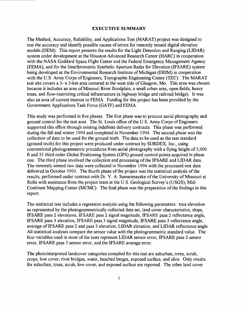
EXECUTIVE SUMMARY
The Method, Accuracy, Reliability, and Applications Test (MARAT) project was designed to test the accuracy and identify possible causes of errors for remotely sensed digital elevation models (DEM). This report presents the results for the Light Detection and Ranging (LIDAR) system under development at the Houston Advanced Research Center (HARC) in cooperation with the NASA Goddard Space Flight Center and the Federal Emergency Management Agency (FEMA), and for the Interferometric Synthetic Aperture Radar for Elevation (IFSARE) system being developed at the Environmental Research Institute of Michigan (ERIM) in cooperation with the U.S. Army Corps of Engineers, Topographic Engineering Center (TEC). The MARAT test site covers a 3- x 3-km area centered at the west side of Glasgow, Mo. This area was chosen because it includes an area of Missouri River floodplain, a small urban area, open fields, heavy trees, and flow-restricting critical infrastructure (a highway bridge and railroad bridge). It was also an area of current interest to FEMA. Funding for this project has been provided by the Government Applications Task Force (GATF) and FEMA.
This study was performed in five phases. The first phase was to procure aerial photography and ground control for the test area. The St. Louis office of the U.S. Army Corps of Engineers supported this effort through existing indefinite delivery contracts. This phase was performed during the fall and winter 1994 and completed in November 1994. The second phase was the collection of data to be used for the ground truth. The data to be used as the test standard (ground truth) for this project were produced under contract by SURDEX, Inc., using conventional photogrammetric procedures from aerial photography with a flying height of 3,000 ft and 31 third order Global Positioning System (GPS) ground control points acquired in phase one. The third phase involved the collection and processing of the IFSARE and LIDAR data. The remotely sensed raw data were collected in November 1994 with the processed test data delivered in October 1995. The fourth phase of the project was the statistical analysis of the results, performed under contract with Dr. V. A. Samaranayake of the University of Missouri at Rolla with assistance from the project team at the U.S. Geological Survey's (USGS), Mid- Continent Mapping Center (MCMC). The final phase was the preparation of the findings in this report.
The statistical test includes a regression analysis using the following parameters: true elevation as represented by the photogrammetrically collected data set, land cover characteristics, slope, IFSARE pass 2 elevations, IFSARE pass 2 signal magnitude, IFSARE pass 2 reflectance angle, IFSARE pass 3 elevation, IFSARE pass 3 signal magnitude, IFSARE pass 3 reflectance angle, average of IFSARE pass 2 and pass 3 elevation, LIDAR elevation, and LIDAR reflectance angle. All statistical analyses compare the sensor value with the photogrammetric standard value. The four variables used in most of the tests represent LIDAR sensor error, IFSARE pass 2 sensor error, IFSARE pass 3 sensor error, and the IFSARE average error.
The photointerpreted landcover categories compiled for this test are suburban, trees, scrub, crops, low cover, river bridges, water, beached barges, exposed surface, and silos. Only results for suburban, trees, scrub, low cover, and exposed surface are reported. The other land cover

categories either had insignificant data quantity or were needed to eliminate data that would bias the test results. Examples of data categories that would bias the test include points under bridges, on water bodies, on silos, or on beached barges that would not be of interest to this test and can be easily eliminated in normal operations by comparison to existing maps and photographs. The technique used in making the photogrammetrically compiled standard should produce data within 0.5 ft Root Mean Square Error (RMSE) accuracy based on ASPRS accuracy standards. These standard data represent the elevation of normal ground beneath any natural ground cover or manmade structure. The LIDAR and IFSARE data were not processed in any special way to eliminate the effects of these above ground phenomena. The simple test synopsis reports the number of points tested, standard deviation, and mean of the errors. The simple regression analysis synopsis reports the degrees of freedom, RMSE, values for the F-test, R- squared value, Y-intercept, and slope of the fitted regression line for each variable used. Assumptions, that are explained in this report, can be made on the applicability of each variable based on these values. The multiple regression analysis synopsis reports the effects of the remaining factors including combinations of some of these factors. Additional statistics are presented that indicate the probability that these factors actually contribute to the reduction of error.
The LIDAR test indicates its ability to detect the ground with a mean error between 1.5 to 3.4 ft and a standard deviation of 1.4 to 8.7 ft when it has a relatively unobstructed view (categories of open ground, low cover, and scrub) of the surface. The LIDAR sensor demonstrated an exceptional ability to penetrate relatively leafless tree cover. The IFSARE test indicates a mean error of between 3.4 and 4.6 ft with a standard deviation of 6.2 to 10.5 ft for relatively unobstructed views of the ground. This sensor did not demonstrate an ability to penetrate leafless trees. Horizontal accuracy cannot be tested because there is nothing in DEM data that is representative of a ground measurable point. All horizontal positions are UTM coordinates only and cannot be verified. Cost data were not reported because of the immaturity of the processes used to produce data for these tests.
This report demonstrates that there are identifiable and possibly correctable patterns within some of the data that were collected and tested. There is evidence that the LIDAR, in its present hardware and software configurations, is calibrated well for all land cover categories with the possible exception of open ground; although the results for this category are not conclusive because of the small number of test points available. With IFSARE there is a much higher probability that error could be reduced using the results of a regression model. In the four categories that the LIDAR demonstrated little systematic error, the IFSARE demonstrated a systematic error of a steady 8 percent to 18 percent possible improvement in the sum of the squares of the errors. This shows a potential for further refinement of the existing configuration of the hardware and software used by IFSARE through calibration to the tested characteristics. The tested characteristics of ground slope and reflectance angle recurred repeatedly as the strongest influence and most probable influence in all of the land use categories for the IFSARE data. The effect was most significant in the open ground category. The potential benefit for this category was close to a 50 percent improvement in accuracy. There was strong correlation with ground slope, reflectance angle , true ground elevation, and signal magnitude in open ground.

Cost data were not reported for this project. LIDAR did not submit data covering the entire test area (which was an allowable option) and IFSARE collected three sets of data over the entire test site. Each organization refined its process and resubmitted data after being informed of potential data irregularities discovered during preliminary tests. All of these factors made it clear that the actual cost associated with collection of these data would not represent costs which would be expected by a mature system.
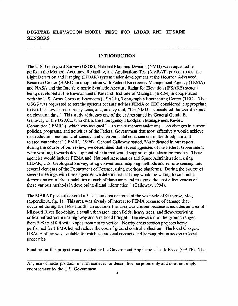
DIGITAL ELEVATION MODEL TEST FOR LIDAR AND IFSARE SENSORS
INTRODUCTION
The U.S. Geological Survey (USGS), National Mapping Division (NMD) was requested to perform the Method, Accuracy, Reliability, and Applications Test (MARAT) project to test the Light Detection and Ranging (LIDAR) system under development at the Houston Advanced Research Center (HARC) in cooperation with Federal Emergency Management Agency (FEMA) and NASA and the Interferometric Synthetic Aperture Radar for Elevation (IFSARE) system being developed at the Environmental Research Institute of Michigan (ERIM) in cooperation with the U.S. Army Corps of Engineers (USAGE), Topographic Engineering Center (TEC). The USGS was requested to test the systems because neither FEMA or TEC considered it appropriate to test their own sponsored systems, and, as they said, "The NMD is considered the world expert on elevation data." This study addresses one of the desires stated by General Gerald E. Galloway of the USAGE who chairs the Interagency Floodplain Management Review Committee (IFMRC), which was assigned "... to make recommendations ... on changes in current policies, programs, and activities of the Federal Government that most effectively would achieve risk reduction, economic efficiency, and environmental enhancement in the floodplain and related watersheds" (IFMRC, 1994). General Galloway stated, "As indicated in our report, during the course of our review, we determined that several agencies of the Federal Government were working towards development of data that would support digital elevation models. These agencies would include FEMA and National Aeronautics and Space Administration, using LIDAR; U.S. Geological Survey, using conventional mapping methods and remote sensing; and several elements of the Department of Defense, using overhead platforms. During the course of several meetings with these agencies we determined that they would be willing to conduct a demonstration of the capabilities of each of these units and to assess the cost effectiveness of these various methods in developing digital information." (Galloway, 1994).
The MARAT project covered a 3- x 3-km area centered at the west side of Glasgow, Mo., (appendix A, fig. 1). This area was already of interest to FEMA because of damage that occurred during the 1993 floods. In addition, this area was chosen because it includes an area of Missouri River floodplain, a small urban area, open fields, heavy trees, and flow-restricting critical infrastructure (a highway and a railroad bridge). The elevation of the ground ranged from 598 to 810 ft with slopes from flat to vertical. Nearby cross section projects being performed for FEMA helped reduce the cost of ground control collection. The local Glasgow USAGE office was available for establishing local contacts and helping obtain access to local properties.
Funding for this project was provided by the Government Applications Task Force (GATF). The
Any use of trade, product, or firm names is for descriptive purposes only and does not imply endorsement by the U.S. Government.

FEMA and TEC offices were active participants in developing the project concept and obtaining funding.
The original scope of the MARAT project was to test the ability of certain new technologies to produce digital elevation models (DEM's). This required the establishment of a suitable test site and test procedures. While establishing the test procedures, a logical extension to the project was to provide statistical evidence of possible spatially based causes for the errors detected. This extension was explained to the participants and accepted. All of the statistics provided could only be calculated using initial assumptions of what these spatially based causes of errors might be. A future expansion of this test may be indicated after the participants study these results.
Appendix A includes illustrations of the data used in this study. There are several instances in the study that reference the difference in characteristics of data in different parts of the study area, or reference "how the data looks". These illustrations should be helpful to the reader in visualizing some of the information presented, as well as in assessing potential applications.
Cost data were not reported for this project. LIDAR did not submit data covering the entire test area (which was an allowable option) and IPS ARE collected three sets of data over the entire test site. Each organization refined its process and resubmitted data after being informed of potential data irregularities discovered during preliminary tests. All of these factors show that the actual cost associated with collection of these data would not represent costs that would be expected by a mature system.

METHODOLOGY
The ground truth (photogrammetrically collected DEM) data were collected under contract. The St. Louis office of the USAGE supported this effort through existing indefinite delivery contracts. The most vital phase needing completion to avoid delays of this project was the procurement of photography. A short time frame existed before having to wait until the thawing of the winter snows. The normal USGS channels for obtaining photography could not have obtained the photography during the fall flying season. The conventional photography was collected in November 1995. It was flown at 3,000 ft above mean ground elevation with a 6-in focal-length camera. The photogrammetrically collected DEM was produced through a contract with Surdex. This DEM was designed to be the most accurate one that was practical to produce from aerial photography. Surdex collected extensive mass points and break lines that were processed through Terramodel software to produce a DEM that will hereafter be referred to as the "standard". This standard is used as the source of ground truth for all tests as agreed to by the original participants.
Ground control was planned and collected in a configuration that would support the LIDAR, IPS ARE, and the conventional photogrammetry. This necessitated the collection of 31 third order accuracy GPS ground stations. The ground control was collected under contract with Michael Baker Jr. Inc. The control to support the LIDAR mission was placed on 8- x 8-ft platforms that were constructed to stand one-half to 1 m above the ground. This was to ensure that these ground control points could be identified in the LIDAR raw data. The LIDAR panels' placements were configured to provide two points at the ends and points at the center of each proposed flight line. The IFSARE points were placed where radar reflectors would be visible during data collection and configured in a crossing pattern through the center of the project as requested by ERIM. The standard photography control points were marked with white paneled crosses and spaced with no more than three models between control points.
The LIDAR mission was flown on November 17, 1994 at 3,000 ft above ground level at an average forward aircraft velocity of 175 mi/h. The coverage of each data swath was 1,500 ft and the horizontal spacing between data samples (laser strikes on the ground) was approximately 10 ft. The differential kinematic baseline distance between the airborne GPS receiver and the ground-based GPS reference receiver was approximately 10 km over the Glasgow site. LIDAR data have been submitted twice during this test in an effort to refine the processing of these data.
The IFSARE mission was flown at 40,000 ft with a 10-km wide collection swath capable of collecting this area in a single flight. The aircraft speed was approximately 480 mi/h with a collection rate of 120 km2/min. The reported ground sample distance is approximately 10 m, although this is actually an average of signals returned at approximately 2.4-m increments. IFSARE data were collected three times over this site as the sensor has been refined. Two of these sets were flown on the same day and are reported in this test. Additional information about the LIDAR and IFSARE sensors can be found in appendix B.
Some "dropout" elevations that were obviously erroneous were observed in the IFSARE and

LIDAR test data. These were obvious because they were below the lowest elevations as determined from the USGS l:24,000-scale maps. To avoid unrealistic test results, these data points were adjusted to a value equal to the known lowest legitimate elevation, or given a value that would avoid their use in this test.
Each organization was allowed to submit up to three data sets, each using a different configuration of control. One of the results of this test was intended to be the determination of the effect of different ground control configurations. This result was not realized because of time constraints and system maturity. HARC requested the positions for all ground control before submitting their first official data set. The ground control was requested to finalize the calibration needed for a successful mosaic of data from multiple flights. This mosaicing process had not been performed previously on LIDAR data. The final test data submitted by HARC (LIDAR) were two flight lines wide and included less than half of the full 3- x 3-km test area (appendix A, fig. 2). This was agreeable with all parties to the test. The EFSARE test was performed at the opposite control configuration extreme. Although EFSARE was flown twice and collected three sets of data, two data sets were submitted but neither used any local (test site) ground control in the calculations. The only control points used were at the airports where the plane took off and landed. All ground control positions were held exclusively by the author and only distributed on request from the test parties.
The data for both remote sensors were originally scheduled for delivery to Mid-Continent Mapping Center (MCMC) by April 1, 1995. Both ERIM and HARC had difficulty with georeferencing their DEM data sets and calibrating their systems. ERIM reflew the mission because of GPS multipath problems. Both companies asked for extensions on the data delivery schedule, which were granted because the purpose of these tests is to understand the potential of these systems. Due to georeferencing and mosaicing concerns at HARC, it requested all 5 LIDAR ground control points within their mosaic area before delivering their first and final test data set. ERIM delivered its final data set before requesting any ground control. ERIM's final DEM data delivery consists of three data sets; two are from independent flights over the test areas, and the third is the average values of the other two. ERIM has indicated these data sets still contain about a 5-m horizontal bias. Because of resource constraints, it did not provide corrected data for this test. Each organization submitted data using only one configuration of ground control (although each organization used a different one). The test DEM data were not delivered to MCMC until October 1995. These systems are now reaching maturity and this test site has aided both developmental activities in the refinement of their systems.
Dr. V. A. Samaranayake, an associate professor from the University of Missouri at Rolla, was contracted as a consultant for the statistical analysis of these data. A regression analysis procedure using the SAS software package was used to determine the accuracy of these systems as well as to determine the effects of some error contributing factors. The initial results of these tests have already been used in the systems' calibration. A synopsis of these results is included in the body of this report with the full statistical data available on request.
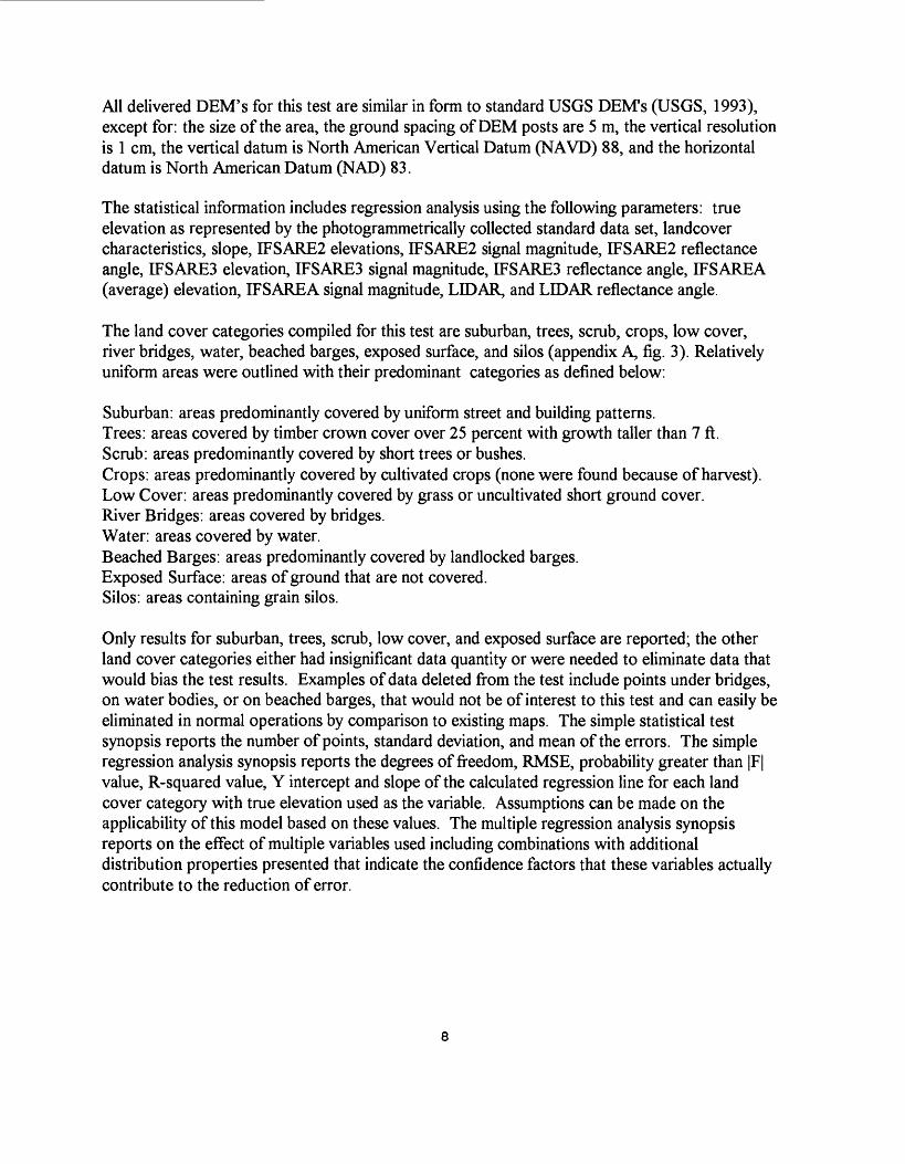
All delivered OEM's for this test are similar in form to standard USGS OEM's (USGS, 1993), except for: the size of the area, the ground spacing of DEM posts are 5 m, the vertical resolution is 1 cm, the vertical datum is North American Vertical Datum (NAVD) 88, and the horizontal datum is North American Datum (NAD) 83.
The statistical information includes regression analysis using the following parameters: true elevation as represented by the photogrammetrically collected standard data set, landcover characteristics, slope, IFSARE2 elevations, IFSARE2 signal magnitude, IFSARE2 reflectance angle, IFSARE3 elevation, IFSARE3 signal magnitude, IFSARE3 reflectance angle, IFSAREA (average) elevation, IFSAREA signal magnitude, LIDAR, and LIDAR reflectance angle.
The land cover categories compiled for this test are suburban, trees, scrub, crops, low cover, river bridges, water, beached barges, exposed surface, and silos (appendix A, fig. 3). Relatively uniform areas were outlined with their predominant categories as defined below:
Suburban: areas predominantly covered by uniform street and building patterns.Trees: areas covered by timber crown cover over 25 percent with growth taller than 7 ft.Scrub: areas predominantly covered by short trees or bushes.Crops: areas predominantly covered by cultivated crops (none were found because of harvest).Low Cover: areas predominantly covered by grass or uncultivated short ground cover.River Bridges: areas covered by bridges.Water: areas covered by water.Beached Barges: areas predominantly covered by landlocked barges.Exposed Surface: areas of ground that are not covered.Silos: areas containing grain silos.
Only results for suburban, trees, scrub, low cover, and exposed surface are reported; the other land cover categories either had insignificant data quantity or were needed to eliminate data that would bias the test results. Examples of data deleted from the test include points under bridges, on water bodies, or on beached barges, that would not be of interest to this test and can easily be eliminated in normal operations by comparison to existing maps. The simple statistical test synopsis reports the number of points, standard deviation, and mean of the errors. The simple regression analysis synopsis reports the degrees of freedom, RMSE, probability greater than |F| value, R-squared value, Y intercept and slope of the calculated regression line for each land cover category with true elevation used as the variable. Assumptions can be made on the applicability of this model based on these values. The multiple regression analysis synopsis reports on the effect of multiple variables used including combinations with additional distribution properties presented that indicate the confidence factors that these variables actually contribute to the reduction of error.

SIMPLE STATISTICAL ANALYSIS
Simple statistics represent the actual performance of these sensors in the Glasgow area. Speculation about how these sensors will perform in other areas of the country can only be assumed through the test of a single small site. These test data were subsets of the full data sets collected. The data that were tested for all of the statistical analyses were subsampled to one- fourth of the points collected by selecting every other point from every other row of data from the submitted DEM's. This allowed future availability of independent data for testing calibration parameters obtained from these and subsequent tests. The low cover and open ground areas should indicate the true potential of the sensors to detect the position of the object "sensed". These particular areas provide test data that are not influenced by features found above the ground.
It is important to realize that the standard data set was intended to represent the elevation of the normal ground level and not elevations on top of buildings, trees, bridges, or any other object that protrudes from the normal ground surface. The IFSARE and LEDAR data represent whatever returned the most prominent signal from each sample. It should also be noted that for statistical reasons the standard data set was assumed to represent ground truth, but in reality these data should be considered to be equivalent to the accuracy expected from 1.5 ft contours. This means that 90 percent of the elevations are considered to be accurate within 0.75 ft (approximately 0.5 ft RMSE), where the ground is clearly visible to the photogrammetrist. This assumption is consistent with the procedures recommended, and the mapping standards published by the American Society of Photogrammetry and Remote Sensing (ASPRS, 1990).
Unfortunately, the mosaic area chosen by HARC for the LEDAR sensor's test area was very limited in the open ground land cover area. Although the test results were very good, the test procedures yielded only 26 points for use in this test. It is debatable if this result is significant. Because of the lack of open ground test points, the low cover area's test results are much more significant. The LIDAR sensor supplied over 8,000 points and the IFSARE supplied over 38,000 points for this land cover category. Again, it should be noted that the LEDAR test was performed only over a limited portion of the area because of production constraints at HARC, whereas the IFSARE supplied coverage for the entire 3 km2 site. Because of difference in coverages, two tables are provided throughout this report for each statistical test. One table is for the results of all points available in the full test area (table 1) and the other is for the limited results within the area outlined by the LIDAR collection (table 2).
The results of the low cover area for the full coverage test (table 1) indicate that the LIDAR provided data with a mean error of 2.1 ft and the IFSARE provided data with a mean error of 4.3 and 4.6 ft. The IFSARE tested slightly better in the open ground area than it did for the low cover area with a mean error of 3.8 ft. The LIDAR also showed an improvement over the low cover area with the limited set obtaining a mean error of-1.5 ft. The standard deviation of the errors in the low cover area were 8.7 ft for the LIDAR and 8.1 to 10.5 ft for the IFSARE. The results in the scrub areas were LIDAR obtaining 3.4 ft mean and 6.5 ft standard deviation and the IFSARE obtaining 3.5 and 3.4 ft means and 7.9 and 7.6 ft standard deviations.

When the limited data set (table 2) is used, there is more difference in the results from the two sensors. The IFSARE results in the low cover area are 8.1 and 9.6 ft mean error in these areas. The standard deviation is also higher at 12.2 and 16.8 ft. The images of the coverage of the LIDAR (appendix A, fig. 2) compared to the photogrammetric standard (appendix A, fig. 4) shows an obvious difference between the limited data set and full data set results. The LIDAR data were all collected in the more difficult terrain with steep sidehills, heavy timber, and the town. Discussion in the simple regression and multiple regression analysis sections will point out some of the factors influencing accuracy that will help explain the effect of these factors on the accuracy of the IFSAR data. This portion of the study simply points out that the full and limited areas are not homogeneous and the area covered by LIDAR is the more difficult area for the IFSARE sensor. This is also evident for the open ground and scrub categories with considerably higher means and standard deviations within the limited set.
Areas covered or partially covered by trees had a distinct effect on the IFSARE accuracy. In areas classified as trees, the IFSARE mean error from the full data set increased to 27.6 and 26.8 ft. This is consistent with what might be the expected crown height for the trees, which are mostly oak in this area. An informal sample indicated the trees reached heights of 50 ft to 80 ft on this site. The same effect can be seen in the suburban areas, where the IFSARE mean error was 9.7 and 10.2 ft. This does not show as high a mean error as in the trees, but the tree growth in this area covers a lower percentage of the area. These results indicate that the IFSARE is probably penetrating very little of the nearly leafless tree crown.
The suburban area presented a particularly difficult area for these tests because the standard elevation model used for the test was required to represent the land surface and intentionally was not representative of the buildings. The LIDAR returned results that were expected, considering the normal distribution and height of buildings and trees in this land cover category. Its mean error was slightly higher at 3.7 ft than the low cover areas and the standard deviation was much higher at 15.7 feet. This indicates that the visible ground was probably detected at about the same accuracy level as it was in the low cover areas. In all probability it also accurately detected the elevation of the tops of the building although this was not tested. The result of these two assumptions would yield the higher standard deviation results reported. The IFSARE showed a different result in the suburban area. Its results were 9.7 to 10.2 ft means and all.6toll.7ft standard deviation for the full data set and similar results for the limited data set. This was a lower standard deviation than might have been expected, but with a higher mean. This seems to indicate that the overall elevation in this area was biased, which would be consistent with this sensor detecting the elevation of the tops of the tree cover found in abundance in the suburban Glasgow area.
10
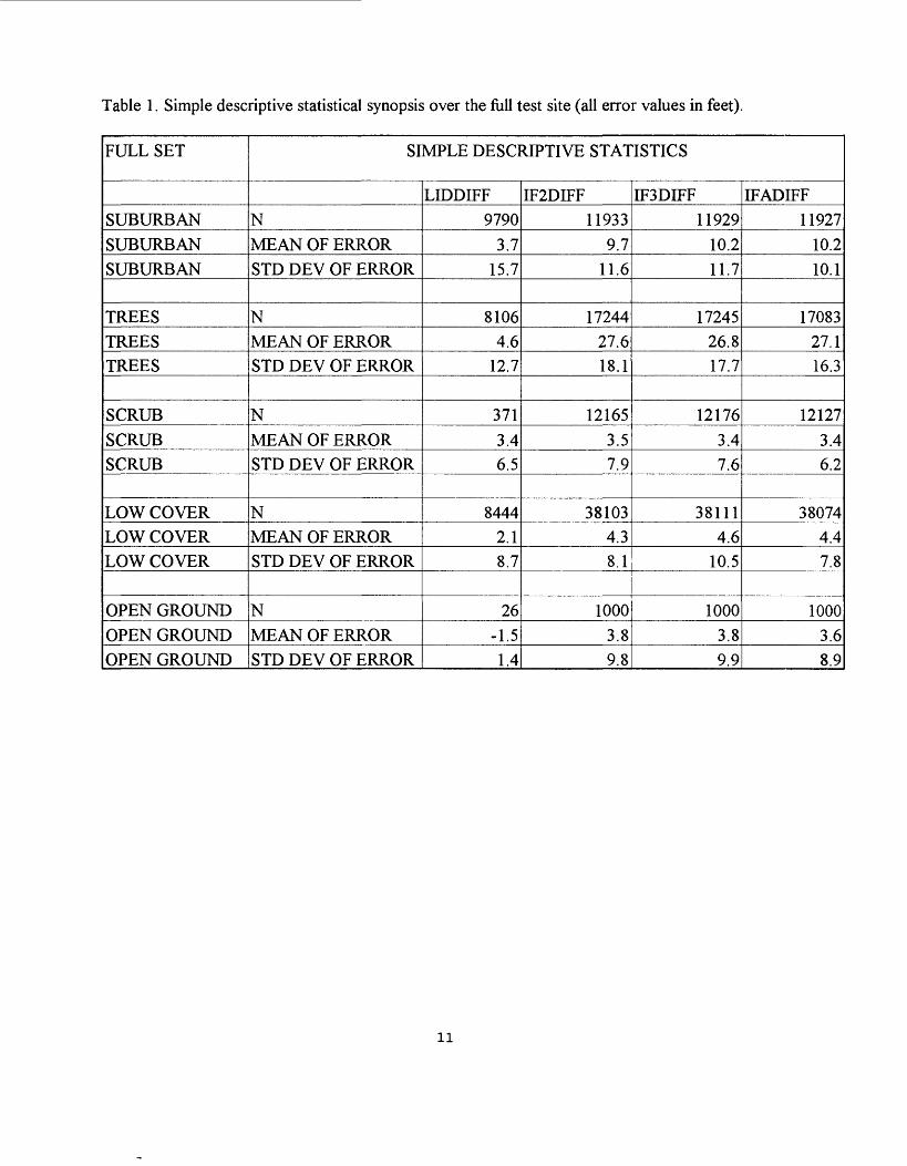
Table 1. Simple descriptive statistical synopsis over the full test site (all error values in feet).
FULL SET
SUBURBANSUBURBANSUBURBAN
TREESTREESTREES
SCRUBSCRUBSCRUB
LOW COVERLOW COVERLOW COVER
OPEN GROUNDOPEN GROUNDOPEN GROUND
SIMPLE DESCRIPTIVE STATISTICS
NMEAN OF ERRORSTD DEV OF ERROR
NMEAN OF ERRORSTD DEV OF ERROR
NMEAN OF ERRORSTD DEV OF ERROR
NMEAN OF ERRORSTD DEV OF ERROR
NMEAN OF ERRORSTD DEV OF ERROR
LIDDIFF9790
3.715.7
81064.6
12.7
3713.46.5
84442.18.7
26-1.5
1.4
IF2DIFF11933
9.711.6
1724427.618.1
121653.57.9
381034.38.1
10003.89.8
IF3DIFF11929
10.211.7
1724526.817.7
121763.47.6
381114.6
10.5
10003.89.9
IFADIFF11927
10.210.1
1708327.116.3
121273.46.2
380744.47.8
10003.68.9
11
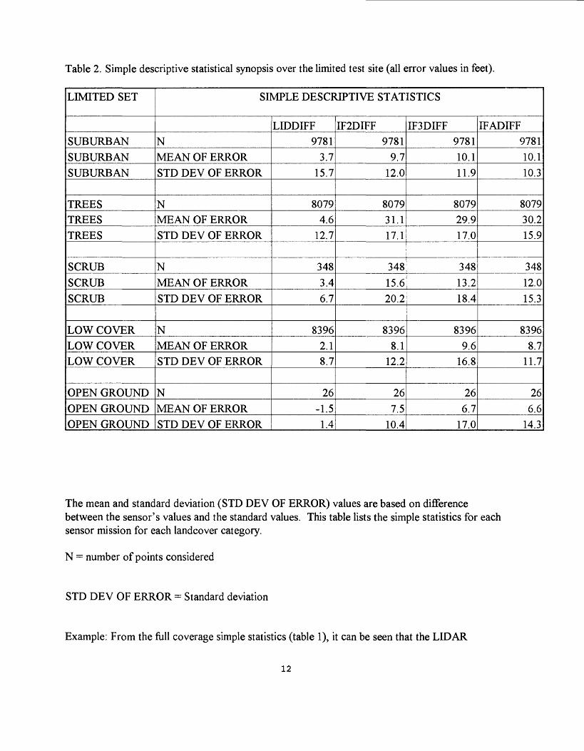
Table 2. Simple descriptive statistical synopsis over the limited test site (all error values in feet).
LIMITED SET
SUBURBANSUBURBANSUBURBAN
TREESTREESTREES
SCRUB
SCRUBSCRUB
LOW COVERLOW COVERLOW COVER
OPEN GROUND
OPEN GROUNDOPEN GROUND
SIMPLE DESCRIPTIVE STATISTICS
NMEAN OF ERRORSTD DEV OF ERROR
NMEAN OF ERRORSTD DEV OF ERROR
N
MEAN OF ERRORSTD DEV OF ERROR
NMEAN OF ERRORSTD DEV OF ERROR
NMEAN OF ERRORSTD DEV OF ERROR
LIDDIFF9781
3.715.7
80794.6
12.7
348
3.46.7
8396
2.18.7
26-1.5
1.4
IF2DIFF9781
9.712.0
807931.117.1
348
15.620.2
83968.1
12.2
26
7.510.4
IF3DIFF978110.111.9
807929.917.0
348
13.218.4
83969.6
16.8
26
6.717.0
IFADIFF978110.110.3
807930.215.9
348
12.015.3
8396
8.711.7
266.6
14.3
The mean and standard deviation (STD DEV OF ERROR) values are based on difference between the sensor's values and the standard values. This table lists the simple statistics for each sensor mission for each landcover category.
N = number of points considered
STD DEV OF ERROR = Standard deviation
Example: From the full coverage simple statistics (table 1), it can be seen that the LIDAR
12

mission area had 9,781 points in the suburban land cover area with a mean error of 3.7 ft and a standard deviation of 15.7 ft for this error.
13

SIMPLE REGRESSION ANALYSIS
The simple linear regression model attempts to explain sensor error as a linear function of the true elevation. If the sensors give an unbiased estimate of the true elevation, then sensor error should consist of purely random noise, which would be indicated by RMSE values close to the values given by the standard deviation from the simple statistics. The level of variation of this "noise" would be an indication of how "precise" the sensors are.
On the other hand, if there is a constant bias across all elevations, then in addition to the random noise, sensor error would have a constant component. One can represent such a situation by the model yi =a+e i , where yi is the sensor error at point i, a is the constant bias term, and e^ is the random noise component of the sensor error.
Another scenario arises if sensor error has a component that is dependent on the true elevation. Then we write %=<* +$xi +e i , where x± is the true elevation at point i and 3 is a parameter that scales the influence of x. on the sensor error yi . Poor calibration of sensor instruments for a given type of land use can result in a situation as above where constant or elevation dependent bias are present. If so, then the estimated regression model yields a way to remove such bias by using the relationship ^= (y^-a) /3 .
Sensor error can have other components in addition to the noise, constant bias, and elevation related bias indicated in the simple linear regression model. It is possible that land slope can affect the accuracy of the sensor estimates. In this case, the regression model should include a term that introduces land slope as another independent variable. If the influence of factors such as signal magnitude and reflectance angle on the sensor error are to be modeled, then these should also be included in the regression model. Such considerations lead to the multiple regression model reported later in this study.
The simple linear regression analysis has to be compared with the results from the simple test. Tables 3 and 4 are comparisons of the simple statistics standard deviation with the simple regression analysis RMSE. The RMSE reflects the variation of the sensor error that is not eliminated by accounting for constant and elevation related bias. If any systematic error present in the sensor estimates is completely accounted for by the x+pxi component of the model, then the residual error present, after fitting the simple linear model, is a predicted value of the random noise component ei at each point. The residual errors have zero mean and RMSE is their standard deviation. Thus, RMSE reflects the variability of the random noise about zero. If RMSE is small, then the residual error (that is, unsystematic error) is near zero for almost all points. This implies that the random noise component is small (Dr. V. A. Samaranayake, written commun., 1996).
14
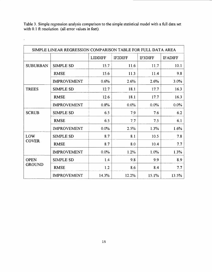
Table 3. Simple regression analysis comparison to the simple statistical model with a full data set with 0.1 ft resolution (all error values in feet).
SIMPLE LINEAR REGRESSION COMPARISON TABLE FOR FULL DATA AREA
SUBURBAN
TREES
SCRUB
LOW COVER
OPEN GROUND
SIMPLE SD
RMSE
IMPROVEMENT
SIMPLE SD
RMSE
IMPROVEMENT
SIMPLE SD
RMSE
IMPROVEMENT
SIMPLE SD
RMSE
IMPROVEMENT
SIMPLE SD
RMSE
IMPROVEMENT
LIDDIFF
15.7
15.6
0.6%
12.7
12.6
0.8%
6.5
6.5
0.0%
8.7
8.7
0.0%
1.4
1.2
14.3%
IF2DIFF
11.6
11.3
2.6%
18.1
18.1
0.0%
7.9
7.7
2.5%
8.1
8.0
1.2%
9.8
8.6
12.2%
IF3DIFF
11.7
11.4
2.6%
17.7
17.7
0.0%
7.6
7.5
1.3%
10.5
10.4
1.0%
9.9
8.4
15.1%
IFADIFF
10.1
9.8
3.0%
16.3
16.3
0.0%
6.2
6.1
1.6%
7.8
7.7
1.3%
8.9
7.7
13.5%
15
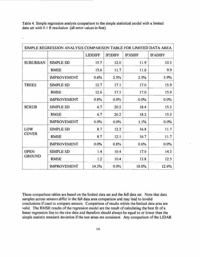
Table 4. Simple regression analysis comparison to the simple statistical model with a limited data set with 0.1 ft resolution (all error values in feet).
SIMPLE REGRESSION ANALYSIS COMPARISON TABLE FOR LIMITED DATA AREA
SUBURBAN
TREES
SCRUB
LOW COVER
OPEN GROUND
SIMPLE SD
RMSE
IMPROVEMENT
SIMPLE SD
RMSE
IMPROVEMENT
SIMPLE SD
RMSE
IMPROVEMENT
SIMPLE SD
RMSE
IMPROVEMENT
SIMPLE SD
RMSE
IMPROVEMENT
LIDDIFF
15.7
15.6
0.6%
12.7
12.6
0.8%
6.7
6.7
0.0%
8.7
8.7
0.0%
1.4
1.2
14.3%
IF2DIFF
12.0
11.7
2.5%
17.1
17.1
0.0%
20.2
20.2
0.0%
12.2
12.1
0.8%
10.4
10.4
0.0%
IF3DIFF
11.9
11.6
2.5%
17.0
17.0
0.0%
18.4
18.2
1.1%
16.8
16.7
0.6%
17.0
13.8
18.8%
IFADIFF
10.3
9.9
3.9%
15.9
15.9
0.0%
15.3
15.3
0.0%
11.7
11.7
0.0%
14.3
12.5
12.6%
These comparison tables are based on the limited data set and the full data set. Note that data samples across sensors differ in the full data area comparison and may lead to invalid conclusions if used to compare sensors. Comparison of results within the limited data area are valid. The RMSE results of the regression model are the result of calculating the best fit of a linear regression line to the raw data and therefore should always be equal to or lower than the simple statistic standard deviation if the test areas are consistent. Any comparison of the LIDAR
16

and IFSARE sensor capabilities can only be made using the limited data set where the results represent errors over a common test area. Appendix A, figures 2 and 5 show the area covered by each sensor. The full data set covered by the standard data represents a more common area of floodplain that includes both the flat open areas on one side of the river and the steeper, tree covered area on the other. It is evident in the multiple regression analysis of the IPS ARE data discussed later, that the slope of the ground was an influencing factor in the regression model for the low cover and open ground areas. Most of the data points in these land cover categories that were used in the full data set were from the floodplain on the west side of the river where the ground is almost flat and is not included in the limited data set. The ground in the limited area has much steeper slope characteristics than that found in the full data set, which accounts for the higher IFSARE RMSE's.
The simple linear regression analysis assumed the actual ground elevation as the variable. If this variable exerted a strong influence on the data, the RMSE value of this model would show a significant decrease from that of the standard deviation in shown simple statistics. The comparison tables (tables 3 and 4) do not indicate such a strong trend.
Additional information can be discovered by studying the simple linear regression analysis of variance data that are synopsised in tables 5 and 6. The values in the synopsis indicate the relative effect that the selected variable has on the accuracy of the test results and the significance that can be attributed to this result. High utility of the model is indicated by a very low value of the Prob>F. The fact that the RMSE does not indicate a significant reduction over the standard deviation of the simple statistics, eliminates the elevation as being a very useful error factor. The expected benefit from using the regression model can be determined by looking at the R-squared value. This value is the ratio of the sum of the squares of the errors found in the raw data to the sum of the square of the errors after application of the regression formula. The extremely small values of R-squared reported in these tests indicate that little improvement in the accuracy of these test results is possible using the actual elevation as the variable in the regression model.
17

Table 5. Simple linear regression synopsis using the limited data set with RMSE and dependent mean in feet.
Limited set
SUBURBANSUBURBANSUBURBANSUBURBANSUBURBAN
SUBURBANSUBURBANSUBURBANSUBURBAN
TREESTREESTREESTREESTREES
TREESTREESTREESTREES
SCRUBSCRUBSCRUBSCRUBSCRUB
SCRUBSCRUBSCRUBSCRUB
SIMPLE LINEAR REGRESSION
DFRMSEPROB>FR-SQUAREDEP MEAN OF ERRORY-INTY PROB>|T|SLOPESLOPE P>|T|
DFRMSEPROB>FR-SQUAREDEP MEAN OF ERRORY-INTYPROB>|T|SLOPESLOPE P>|T|
DFRMSEPROB>FR-SQUAREDEP MEAN OF ERRORY-INTYPROB>|T|SLOPESLOPE P>|T|
LIDDIFF978015.6
0.00010.0095
3.7
273.73550.0001-0.0340.0001
807812.6
0.00010.0035
4.6
-54.43740.00390.01470.0001
3476.7
0.14150.0062
3.4
-65.28380.33220.01480.1415
IF2DIFF978011.7
0.00010.0425
9.8
-285.0710.00010.05490.0001
807817.1
0.54370
31.1
295.85330.00010.00230.5437
34720.2
0.43190.0018
15.6
316.27170.1216
-0.02390.4319
IF3DIFF978011.6
0.00010.0502
10.1
-312.73830.00010.05930.0001
807817
0.00490.001
29.9
-370.10160.0001
-0.01040.0049
34718.2
0.0010.0309
13.2
739.59980.0001
-0.09080.001
IFADIFF9780
9.90.00010.0656
10.1
-306.78210.00010.05860.0001
807815.9
0.80790
30.2
308.18320.0001
-0.00080.8079
34715.3
0.76650.0003
12
74.3370.63010.00680.7765
18
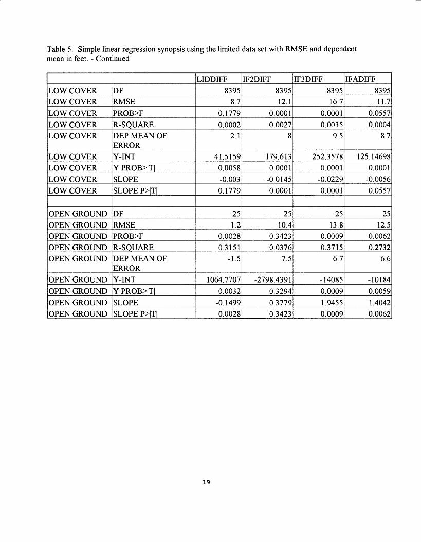
Table 5. Simple linear regression synopsis using the limited data set with RMSE and dependent mean in feet. - Continued
LOW COVERLOW COVERLOW COVERLOW COVERLOW COVER
LOW COVERLOW COVERLOW COVERLOW COVER
OPEN GROUNDOPEN GROUNDOPEN GROUNDOPEN GROUNDOPEN GROUND
OPEN GROUNDOPEN GROUNDOPEN GROUNDOPEN GROUND
DFRMSEPROB>FR-SQUAREDEP MEAN OF ERRORY-INTY PROB>|T|SLOPESLOPE P>|T|
DFRMSEPROB>FR-SQUAREDEP MEAN OF ERRORY-INTY PROB>|T|SLOPESLOPE P>|T|
LIDDIFF8395
8.70.17790.0002
2.1
41.51590.0058-0.0030.1779
251.2
0.00280.3151
-1.5
1064.77070.0032
-0.14990.0028
IF2DIFF839512.1
0.00010.0027
8
179.6130.0001
-0.01450.0001
2510.4
0.34230.0376
7.5
-2798.43910.32940.37790.3423
IF3DIFF839516.7
0.00010.0035
9.5
252.35780.0001
-0.02290.0001
2513.8
0.00090.3715
6.7
-140850.00091.94550.0009
IFADIFF839511.7
0.05570.0004
8.7
125.146980.0001
-0.00560.0557
2512.5
0.00620.2732
6.6
-101840.00591.40420.0062
19
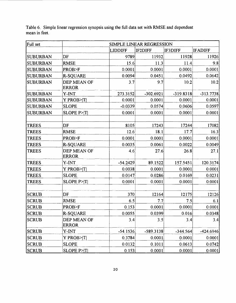
Table 6. Simple linear regression synopsis using the full data set with RMSE and dependent mean in feet.
Full set
SUBURBANSUBURBANSUBURBANSUBURBANSUBURBAN
SUBURBANSUBURBANSUBURBANSUBURBAN
TREESTREESTREESTREESTREES
TREESTREESTREESTREES
SCRUBSCRUBSCRUBSCRUBSCRUB
SCRUBSCRUBSCRUBSCRUB
SIMPLE LINEAR REGRESSION
DFRMSEPROB>FR-SQUAREDEP MEAN OF ERRORY-INTY PROB>|T|SLOPESLOPE P>|T|
DFRMSEPROB>FR-SQUAREDEP MEAN OF ERRORY-INTY PROB>|T|SLOPESLOPE P>|T|
DFRMSEPROB>FR-SQUAREDEP MEAN OF ERRORY-INTY PROB>|T|SLOPESLOPE P>|T|
LIDDIFF978915.6
0.00010.0094
3.7
273.31520.0001
-0.03390.0001
810512.6
0.00010.0035
4.6
-54.24290.00380.01470.0001
3706.5
0.1530.0055
3.4
-54.15360.37840.0132
0.153
IF2DIFF11932
11.30.00010.0451
9.7
-302.69210.00010.05740.0001
1724318.1
0.00010.0061
27.6
89.15220.00010.02860.0001
121647.7
0.00010.0399
3.5
-589.31380.00010.10110.0001
IF3DIFF11928
11.40.00010.0492
10.2
-319.83180.00010.06060.0001
1724417.7
0.00010.0022
26.8
157.54510.00010.01690.0001
121757.5
0.00010.016
3.4
-344.5640.00010.06130.0001
IFADIFF11926
9.80.00010.0642
10.2
-313.77380.00010.05970.0001
1708216.3
0.00010.0049
27.1
120.31740.00010.02310.0001
121266.1
0.00010.0348
3.4
-424.69460.00010.07420.0001
20

Table 6. Simple linear regression synopsis using the full data set with RMSE and dependent mean in feet. - Continued
LOW COVERLOW COVERLOW COVERLOW COVERLOW COVER
LOW COVERLOW COVERLOW COVERLOW COVER
OPEN GROUNDOPEN GROUNDOPEN GROUNDOPEN GROUNDOPEN GROUND
OPEN GROUNDOPEN GROUNDOPEN GROUNDOPEN GROUND
DFRMSEPROB>FR-SQUAREDEP MEAN OF ERRORY-INTY PROB>|T|SLOPESLOPE P>|T|
DFRMSEPROB>FR-SQUAREDEP MEAN OF ERRORY-INTY PROB>|T|SLOPESLOPE P>|T|
LIDDIFF8443
8.70.20570.0002
2.1
40.06730.0071
-0.00270.2057
251.2
0.00280.3151
-1.5
1064.77070.0032
-0.14990.0028
IF2DIFF38102
80.00010.0237
4.3
-144.70250.00010.02920.0001
9998.6
0.00010.2334
3.8
856.9720.0001
-0.12950.0001
IF3DIFF38110
10.40.00010.0173
4.6
-160.37880.00010.03220.0001
9998.4
0.00010.2816
3.8
947.89010.0001
-0.14390.0001
IFADIFF38073
7.7_ 0.0001
0.03364.4
-170.4240.00010.03350.0001
9997.7
0.00010.264
3.6
827.27580.0001
-0.12520.0001
LIDDIFF = difference between the LIDAR elevation and the standard elevation
IF2DIFF = difference between the second pass IFSARE elevation and the standard elevation
IF3DIFF = difference between the third pass IFSARE elevation and the standard elevation
IFADIFF = difference between the average IFSARE elevation and the standard elevation
DF = Degrees of Freedom of test data
21

RMSE = Root Mean Square Error
Prob>F = The p-value of the F-test associated with the simple linear regression model. It is the probability of obtaining an F-value equal to or greater than what is computed for the data, under the hypothesis that the sensor error is not related to true elevation as postulated by the simple linear regression model. In short, small p-values indicate a significant relationship between sensor error and the true elevation (Dr. V.A. Samaranayake, written commun., 1996). For the purposes of this study, any p-value less than or equal to 0.05 is indicative of a significant relationship. However, such a relationship may account for only a small fraction of the variation of the sensor error.
R2 = Coefficient of determination. Indicates the portion of the corrected total variation that is attributed to the fit rather than left to residual error. It is mathematically calculated by dividing the sum of squares of the correction model errors by the total sum of squares. In other words, this is the square of the correlation between the dependent variable and the predicted values. It is also the square of the correlation between the dependent and independent variable (Dr. V.A. Samaranayake, written commun., 1996).
DEP MEAN OF ERROR = Simple mean of the dependent variable.
Y-INT = the Y-intercept of the regression line
Y-PROB>|T| = The p-value for testing the hypothesis that the intercept of the t intercept of the model is zero. Small p-values indicate an intercept that is statistically different from zero. A large p-value indicates that any non-zero estimate of the intercept may be due to "noise" in the data. A statistically significant (non-zero) intercept implies the presence of a constant bias across all elevations (Dr. V.A. Samaranayake, written commun., 1996).
An example of how these factors can indicate areas for concentration in the development of this type of technology occurred after preliminary results of these tests. HARC submitted the first LIDAR data before the mosaic was formed. These data were requested for use in establishing the statistical analysis procedure. Simple linear regression analysis tests were run to observe the modeling procedures and to evaluate the variables to be tested. The initial tests indicated a striking correlation between the TRUE ground elevation and the error in the LIDAR data. This was reported to HARC where a laser calibration value in the math model was found to have been entered for the wrong laser parameters. Even though this value was very close to the proper value, these tests pointed to the problem because of the high probability of association of errors found in relation to the actual ground elevation (that is, the error increased as the elevation above sea level increased). This factor was taken into consideration and corrected for the final data set that was submitted.
22

MULTIPLE REGRESSION ANALYSIS
The analysis of the multiple regression synopsis carries this process one step further and considers variables, in addition to true ground elevations, variables such as ground slope, signal magnitude for IPS ARE, reflectance angle, and various combinations of these variables. This study does not include an analysis of each of these variables separately, although there are indications of the applicability of each within each land cover category. The slope (or linear parameter) associated with each variable indicates the sensitivity of the model to the change in the variable's value. The related Prob>|T| value indicates the necessity of the inclusion of each term in the regression model.
There are additional indications of the sensitivity of each variable that can be demonstrated in graphic form. An example of one of these graphs from the raw analysis is shown in figure 1. This graph can be used to visualize the error trend found in the raw data for the IFSARE pass three in the suburban land cover category. The simple linear regression values found in table 6 indicate a Y-intercept of-307 and a slope of 0.0593 for the best fit regression line. This information can be visualized as a line representing the basic trend of the error that increases with the increase in elevation. The multiple regression analysis breaks this trend down further to analyze the effects of factors other than the elevation of the ground as the possible cause of these errors. These give a numerical representation of the errors for each variable in each land use category. The slope listed for each variable can be visualized as the slope of a trend line through the error plots as the errors relate to each variable. The RMSE value can be visualized as an indicator of the scattering of the data points about these trend lines.
23

IF3DIFF
1000 +
800 +
600
400
2000
+
-200 +I I
-400 + I II
-600 + i--- 6000
The SAS System
-- LANDUSE=1
19:29 Wednesday, November 8,
1995
68
Plot of IF3DIFF*TRUE.
:.. ...
.:..:.:..;.:*;::;:;*;..:;..:;*:.*;#:;::**:;::;#;*.;;::**::;....*.:.
.. '.'
.!..:;.:.!......#;.:;.;;:; *#* .*;*:*;;;;*: **#;; :**;*;;*;*; : *
*#*#. *;; : : :*#»!'. . .
: : : * *
; ;*
#*;*
**;*;***>!«*#;>!«; **;***>!«;*»!«;**;;;**;; ***#»!« *** »!« :****
i; ! '!' '.*': ':': :': '.':: :; *; : *; ******«»*0»00»^ » »;» * * ; » »**»»»*»; ~^
6200
6400
6600
6800
7000
7200
7400
- +
7600
+_
7800
TRUE
NOTE:
4 obs had missing values.
823 obs hidden.
Figure 1. G
raph of IFSAR
E pass three error vs. true elevation found in the suburban (landcover 1) category.
(The size and intensity of the sym
bol represents the density of errors plotted.)
I-
_ (._
8000
8200
24

Tables 7 and 8 represent the potential improvement in the error distribution of the data when the multiple regression model is applied. These tables indicate that the LIDAR data can be improved only slightly in all categories except open ground where the RMSE can be improved by 36 percent. Again, this category is under represented in the LIDAR data so this result is questionable. A similar result is apparent for the IFSARE data where the open ground RMSE improved by 25 percent to 32 percent for the full data set and 44 percent and 50 percent within the limited area. The IFSARE can be improved by 5 percent to 10 percent in the other land cover categories, also.
Table 7. Multiple regression comparison to the simple statistics using the limited data set with error values in feet.
MULTIPLE REGRESSION IMPROVEMENT FOR LIMITED DATA SET
SUBURBAN
TREES
SCRUB
LOW COVER
OPEN GROUND
UNIVARIATE RMSE
MULTIPLE RMSE
IMPROVEMENT
UNIVARIATE RMSE
MULTIPLE RMSE
IMPROVEMENT
UNIVARIATE RMSE
MULTIPLE RMSE
IMPROVEMENT
UNIVARIATE RMSE
MULTIPLE RMSE
IMPROVEMENT
UNIVARIATE RMSE
MULTIPLE RMSE
IMPROVEMENT
LIDDIFF
15.6
15.6
0.0%
12.6
12.5
0.8%
6.7
6.5
3.0%
8.7
8.7
0.0%
1.2
0.9
25.0%
IF2DIFF
11.7
11.3
3.4%
17.1
15.7
8.2%
20.2
19.5
3.5%
12.1
11.0
9.1%
10.4
5.2
50.0%
IF3DIFF
11.6
10.7
11.2%
17.0
15.5
8.8%
18.2
17.2
5.5%
16.7
16.0
4.2%
13.8
6.4
54.6%
25
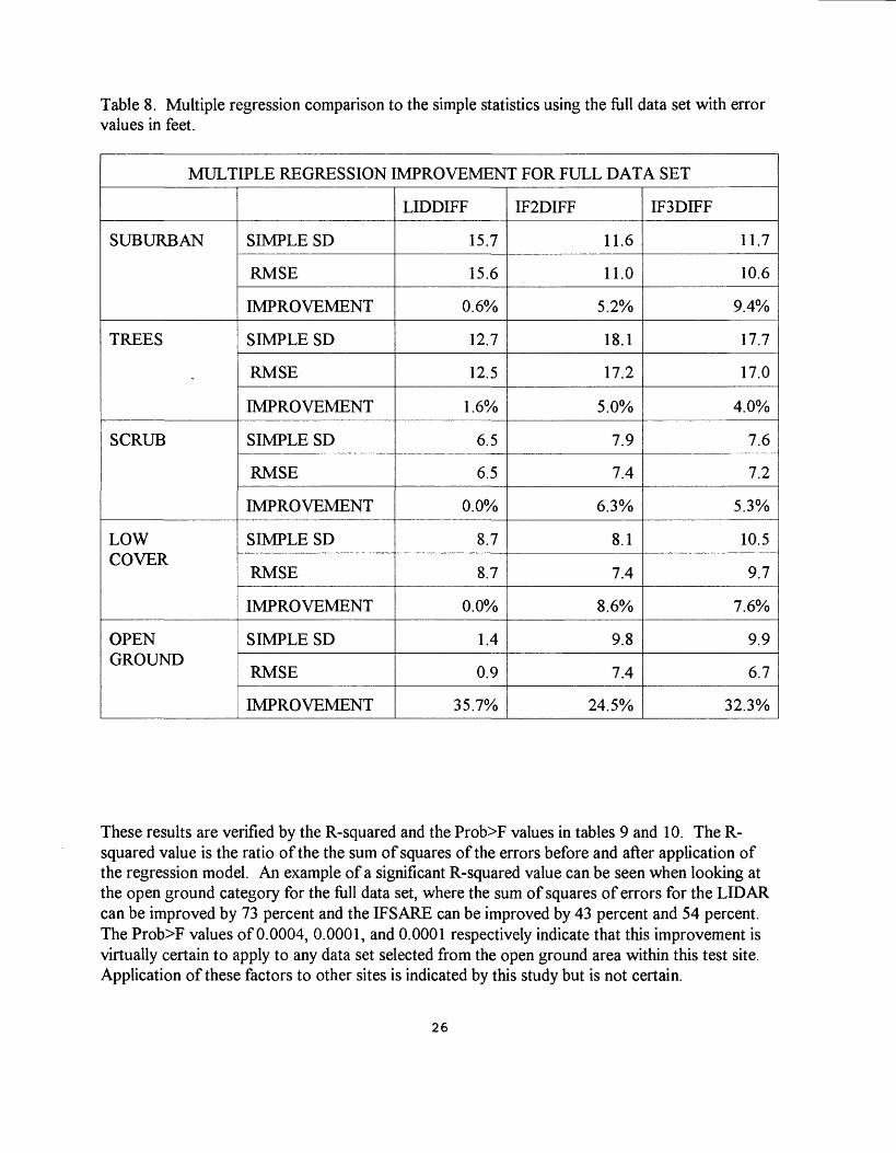
Table 8. Multiple regression comparison to the simple statistics using the full data set with error values in feet.
MULTIPLE REGRESSION IMPROVEMENT FOR FULL DATA SET
SUBURBAN
TREES
SCRUB
LOW COVER
OPEN GROUND
SIMPLE SD
RMSE
IMPROVEMENT
SIMPLE SD
RMSE
IMPROVEMENT
SIMPLE SD
RMSE
IMPROVEMENT
SIMPLE SD
RMSE
IMPROVEMENT
SIMPLE SD
RMSE
IMPROVEMENT
LIDDIFF
15.7
15.6
0.6%
12.7
12.5
1.6%
6.5
6.5
0.0%
8.7
8.7
0.0%
1.4
0.9
35.7%
IF2DIFF
11.6
11.0
5.2%
18.1
17.2
5.0%
7.9
7.4
6.3%
8.1
7.4
8.6%
9.8
7.4
24.5%
IF3DIFF
11.7
10.6
9.4%
17.7
17.0
4.0%
7.6
7.2
5.3%
10.5
9.7
7.6%
9.9
6.7
32.3%
These results are verified by the R-squared and the Prob>F values in tables 9 and 10. The R- squared value is the ratio of the the sum of squares of the errors before and after application of the regression model. An example of a significant R-squared value can be seen when looking at the open ground category for the full data set, where the sum of squares of errors for the LIDAR can be improved by 73 percent and the IFSARE can be improved by 43 percent and 54 percent. The Prob>F values of 0.0004, 0.0001, and 0.0001 respectively indicate that this improvement is virtually certain to apply to any data set selected from the open ground area within this test site. Application of these factors to other sites is indicated by this study but is not certain.
26
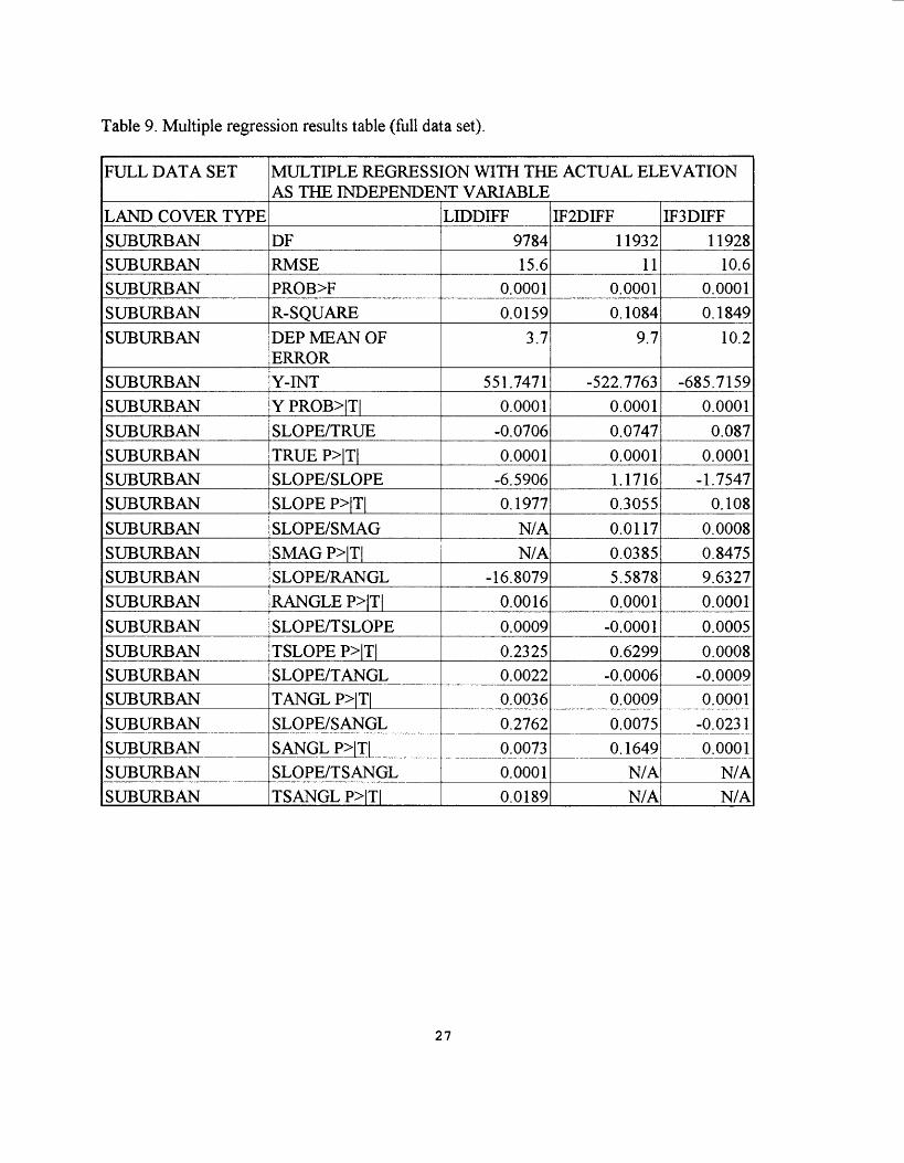
Table 9. Multiple regression results table (full data set).
FULL DAT A SET
LAND COVER TYPESUBURBANSUBURBANSUBURBANSUBURBAN
SUBURBAN
SUBURBANSUBURBAN
SUBURBAN _^SUBURBANSUBURBANSUBURBAN
SUBURBANSUBURBANSUBURBAN
SUBURBAN
SUBURBAN
SUBURBANSUBURBANSUBURBANSUBURBANSUBURBANSUBURBANSUBURBAN
MULTIPLE REGRESSION WITH THE ACTUAL ELEVATION AS THE INDEPENDENT VARIABLE
DFRMSEPROB>FR-SQUARE
DEP MEAN OF ERRORY-INTY PROB>|T|
SLOPE/TRUETRUE P>|T|SLOPE/SLOPESLOPE P>|T|
SLOPE/SMAG
SMAGP>|T|SLOPE/RANGL
RANGLE P>|T|
SLOPE/TSLOPE
TSLOPE P>|T|SLOPE/TANGLTANGL P>|T|SLOPE/SANGLSANGL P>|T|SLOPE/TSANGLTSANGL P>|T|
LIDDIFF978415.6
0.00010.0159
3.7
551.74710.0001
-0.0706
0.0001-6.59060.1977
N/A
N/A-16.8079
0.0016
0.00090.23250.00220.0036
0.27620.00730.00010.0189
IF2DIFF11932
110.00010.1084
9.7
-522.77630.0001
0.07470.00011.17160.3055
0.0117
0.03855.5878
0.0001
-0.00010.6299
-0.00060.0009
0.00750.1649
N/AN/A
IF3DIFF11928
10.60.00010.1849
10.2
-685.71590.0001
0.0870.0001
-1.75470.108
0.00080.84759.6327
0.0001
0.00050.0008
-0.00090.0001
-0.0231
0.0001N/AN/A
27
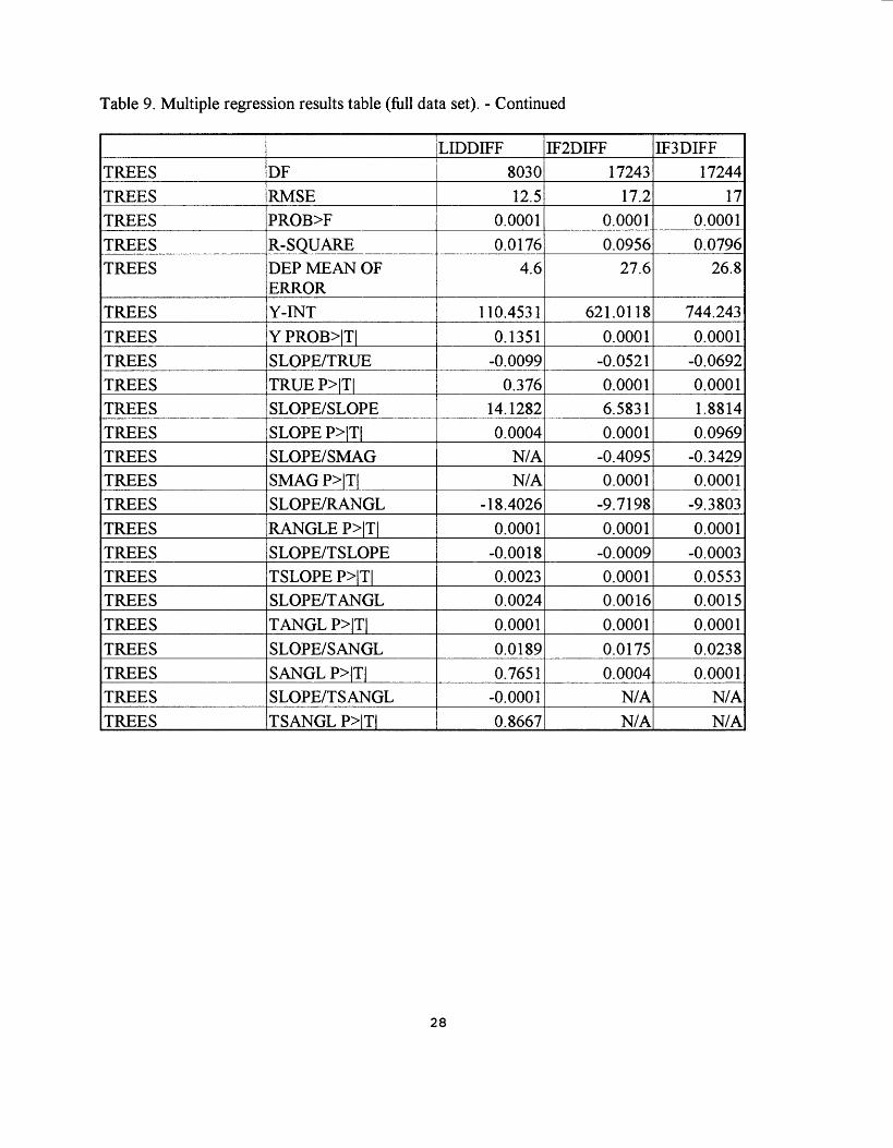
Table 9. Multiple regression results table (full data set). - Continued
TREESTREESTREESTREESTREES
TREESTREESTREESTREESTREESTREESTREESTREESTREESTREESTREESTREESTREESTREESTREESTREESTREESTREES
DFRMSEPROB>FR-SQUAREDEP MEAN OF ERRORY-INTY PROB>|T|SLOPE/TRUETRUE P>|T|SLOPE/SLOPESLOPE P>|T|SLOPE/SMAGSMAG P>|T|SLOPE/RANGLRANGLE P>|T|SLOPE/TSLOPETSLOPE P>|T|SLOPE/TANGLTANGL P>|T|SLOPE/SANGLSANGL P>|T|SLOPE/TSANGLTSANGL P>|T|
LIDDIFF803012.5
0.00010.0176
4.6
110.45310.1351
-0.00990.376
14.12820.0004
N/AN/A
-18.40260.0001
-0.00180.00230.00240.00010.01890.7651
-0.00010.8667
IF2DIFF17243
17.20.00010.0956
27.6
621.01180.0001
-0.05210.00016.58310.0001
-0.40950.0001
-9.71980.0001
-0.00090.00010.00160.00010.01750.0004
N/AN/A
DF3DIFF17244
170.00010.0796
26.8
744.2430.0001
-0.06920.00011.88140.0969
-0.34290.0001
-9.38030.0001
-0.00030.05530.00150.00010.02380.0001
N/AN/A
28

Table 9. Multiple regression results table (full data set). - Continued
SCRUBSCRUBSCRUBSCRUBSCRUB
SCRUBSCRUBSCRUBSCRUBSCRUBSCRUBSCRUBSCRUBSCRUBSCRUBSCRUBSCRUBSCRUBSCRUBSCRUBSCRUBSCRUBSCRUB
DFRMSEPROB>FR-SQUAREDEP MEAN OF ERRORY-INTY PROB>|T|SLOPE/TRUETRUE P>|T|SLOPE/SLOPESLOPE P>|T|SLOPE/SMAGSMAGP>|T|SLOPE/RANGLRANGLE P>|T|SLOPE/TSLOPETSLOPE P>|T|SLOPE/TANGLTANGL P>|T|SLOPE/SANGLSANGL P>|T|SLOPE/TSANGLTSANGL P>|T|
LIDDIFF3396.5
0.00030.0784
3.4
278.15280.1786-0.0360.249
0.38410.9827
N/AN/A
-0.78710.967
0.00020.9463
-0.00010.9874
-0.27240.238
0.00010.2315
IF2DIFF12164
7.40.00010.1217
3.5
-462.5480.00010.07130.0001
17.58090.00010.17630.0001
-2.01010.2845
-0.00290.00010.0004
0.1690.03060.0001
N/AN/A
IF3DIFF12175
7.20.00010.1045
3.4
266.34970.0019-0.0430.0018
17.76330.00010.20320.0001
-12.88110.0001
-0.00290.00010.00210.00010.02840.0001
N/AN/A
29
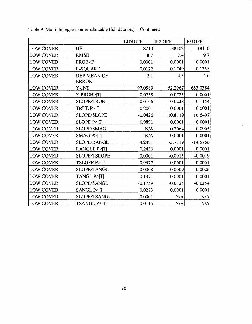
Table 9. Multiple regression results table (full data set). - Continued
LOW COVERLOW COVERLOW COVERLOW COVERLOW COVER
LOW COVERLOW COVERLOW COVERLOW COVERLOW COVERLOW COVERLOW COVERLOW COVERLOW COVERLOW COVERLOW COVERLOW COVERLOW COVERLOW COVERLOW COVERLOW COVERLOW COVERLOW COVER
DFRMSEPROB>FR-SQUAREDEP MEAN OF ERRORY-INTY PROB>|T|SLOPE/TRUETRUE P>|T|SLOPE/SLOPESLOPE P>|T|SLOPE/SMAGSMAGP>|T|SLOPE/RANGLRANGLE P>|T|SLOPE/TSLOPETSLOPE P>|T|SLOPE/TANGLTANGL P>|T|SLOPE/SANGLSANGL P>|T|SLOPE/TSANGLTSANGL P>|T|
LIDDIFF8210
8.70.00010.0122
2.1
97.05890.0738
-0.01060.2001
-0.04260.9891
N/AN/A
4.24810.24360.00010.9377
-0.00080.1371
-0.17590.02730.00010.0115
IF2DIFF38102
7.40.00010.1749
4.3
52.29670.0723
-0.02380.0001
10.81190.00010.20640.0001
-3.71190.0001
-0.00130.00010.00090.0001
-0.01250.0001
N/AN/A
IF3DIFF38110
9.70.00010.1355
4.6
653.03840.0001
-0.11540.0001
16.64070.00010.09050.0001
-14.57660.0001
-0.00190.00010.00260.0001
-0.03540.0001
N/AN/A
30

Table 9. Multiple regression results table (full data set). - Continued
OPEN GROUNDOPEN GROUNDOPEN GROUNDOPEN GROUNDOPEN GROUND
OPEN GROUNDOPEN GROUNDOPEN GROUNDOPEN GROUNDOPEN GROUNDOPEN GROUNDOPEN GROUNDOPEN GROUNDOPEN GROUNDOPEN GROUNDOPEN GROUNDOPEN GROUNDOPEN GROUNDOPEN GROUNDOPEN GROUNDOPEN GROUNDOPEN GROUNDOPEN GROUND
DFRMSEPROB>FR-SQUAREDEP MEAN OF ERRORY-INTY PROB>|T|SLOPE/TRUETRUE P>|T|SLOPE/SLOPESLOPE P>|T|SLOPE/SMAGSMAGP>|T|SLOPE/RANGLRANGLE P>|T|SLOPE/TSLOPETSLOPE P>|T|SLOPE/TANGLTANGL P>|T|SLOPE/SANGLSANGL P>|T|SLOPE/TSANGLTSANGL P>|T|
LIDDIFF250.9
0.00040.7309
-1.5
-5012.92810.0626
0.6950.063
15.41380.876N/AN/A
288.66120.0617
-0.00190.888
-0.04020.0611
-3.96880.01490.00050.0152
IF2DIFF9997.4
0.00010.4344
3.8
3081.93780.0001
-0.48330.0001
-39.81370.00010.42720.0001
-29.80290.00010.00610.00010.00460.00010.02540.1429
N/AN/A
IF3DIFF9996.7
0.00010.5445
3.8
2672.72380.0001
-0.43290.0001
-27.55860.00010.57950.0001
-20.56810.00010.00450.00010.00340.0001
-0.01850.2325
N/AN/A
31
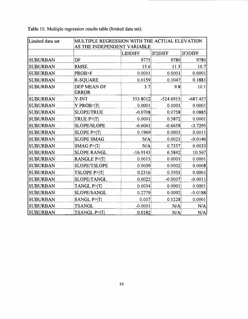
Table 10. Multiple regression results table (limited data set).
Limited data set
SUBURBANSUBURBANSUBURBAN
SUBURBANSUBURBAN
SUBURBANSUBURBANSUBURBANSUBURBANSUBURBAN
SUBURBAN
SUBURBANSUBURBANSUBURBANSUBURBANSUBURBAN
SUBURBANSUBURBANSUBURBANSUBURBAN
SUBURBANSUBURBANSUBURBAN
MULTIPLE REGRESSION WITH THE ACTUAL ELEVATION AS THE INDEPENDENT VARIABLE
DFRMSEPROB>F
R-SQUAREDEP MEAN OF ERRORY-INTY PROB>|T|SLOPE/TRUETRUE P>|T|
SLOPE/SLOPE
SLOPE P>|T|SLOPE SMAGSMAGP>|T|SLOPE RANGLRANGLE P>|T|SLOPE/TSLOPE
TSLOPE P>|T|SLOPE/TANGLTANGL P>|T|SLOPE/SANGL
SANGL P>|T|TSANGLTSANGL P>|T|
LIDDIFF977515.6
0.0001
0.01593.7
553.80120.0001
-0.07080.0001
-6.6061
0.1969
N/AN/A
-16.91430.00150.0009
0.23160.00220.00340.2779
0.007-0.00010.0182
IF2DIFF978011.3
0.0001
0.10479.8
-524.69150.00010.07580.5872
-0.6658
0.0001
0.00210.73576.58420.00010.0002
0.3501-0.00070.00010.0092
0.1228N/AN/A
IF3DIFF978010.7
0.0001
0.188110.1
-687.4570.00010.08850.0001
-3.7295
0.0011-0.01460.003310.5670.00010.0008
0.0001-0.00110.0001
-0.0188
0.0001N/AN/A
32

Table 10. Multiple regression results table (limited data set). - Continued
TREESTREESTREESTREESTREES
TREESTREESTREESTREESTREESTREESTREESTREESTREESTREESTREESTREESTREESTREESTREESTREESTREESTREES
DFRMSEPROB>FR-SQUAREDEP MEAN OF ERRORY-INTY PROB>|T|SLOPE/TRUETRUE P>|T|SLOPE/SLOPESLOPE P>|T|SLOPE SMAGSMAG P>|T|SLOPE RANGLRANGLE P>|T|SLOPE/TSLOPETSLOPE P>|T|SLOPE/TANGLTANGL P>|T|SLOPE/SANGLSANGL P>|T|TSANGLTSANGL P>|T|
LroDIFF800412.5
0.00010.0177
4.6
116.53630.1182
-0.01080.3405
14.09110.0004
N/AN/A
-18.70180.0001
-0.00180.00260.00240.00010.02260.7222
-0.00010.8248
IF2DIFF807815.7
0.00010.159
31.1
4.36640.95320.04530.0001
13.22950.0001
-0.40420.0001
-1.60480.1361
-0.002210.00010.00030.03050.03350.0001
N/AN/A
IF3DIFF
807815.5
0.00010.1694
29.9
229.18490.00170.01230.2495
12.72670.0001
-0.046810.0001
-3.94530.0001-0.0020.00010.00070.0001
0.0270.0001
N/AN/A
33
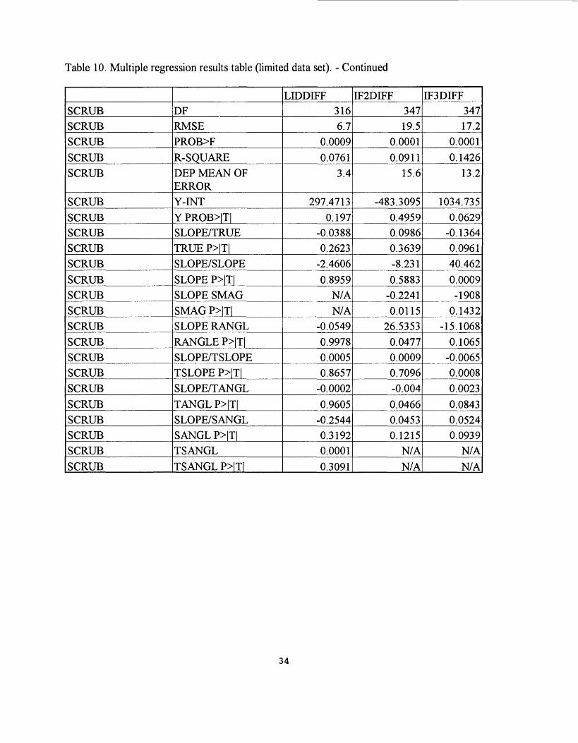
Table 10. Multiple regression results table (limited data set). - Continued
SCRUBSCRUBSCRUBSCRUBSCRUB
SCRUBSCRUBSCRUBSCRUBSCRUBSCRUBSCRUBSCRUBSCRUBSCRUBSCRUBSCRUBSCRUBSCRUBSCRUBSCRUBSCRUBSCRUB
DFRMSEPROB>FR-SQUAREDEP MEAN OF ERRORY-INTY PROB>|T|SLOPE/TRUETRUE P>|T|SLOPE/SLOPESLOPE P>|T|SLOPE SMAGSMAGP>|T|SLOPE RANGLRANGLE P>|T|SLOPE/TSLOPETSLOPE P>|T|SLOPE/TANGLTANGL P>|T|SLOPE/SANGLSANGL P>|T|TSANGLTSANGL P>|T|
LIDDIFF3166.7
0.00090.0761
3.4
297.47130.197
-0.03880.2623
-2.46060.8959
N/AN/A
-0.05490.99780.00050.8657
-0.00020.9605
-0.25440.31920.00010.3091
IF2DIFF34719.5
0.00010.0911
15.6
-483.30950.49590.09860.3639-8.2310.5883
-0.22410.0115
26.53530.04770.00090.7096-0.0040.04660.04530.1215
N/AN/A
IF3DIFF34717.2
0.00010.1426
13.2
1034.7350.0629
-0.13640.096140.4620.0009-1908
0.1432-15.1068
0.1065-0.00650.00080.00230.08430.05240.0939
N/AN/A
34
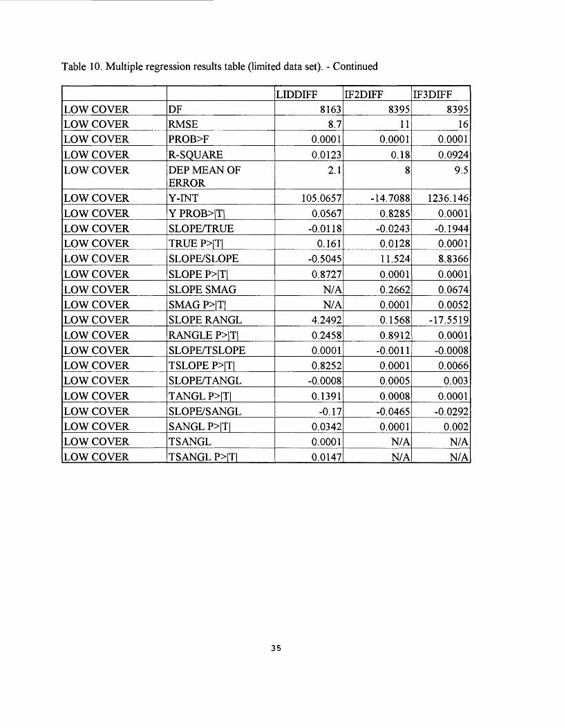
Table 10. Multiple regression results table (limited data set). - Continued
LOW COVERLOW COVERLOW COVERLOW COVERLOW COVER
LOW COVERLOW COVERLOW COVERLOW COVERLOW COVERLOW COVERLOW COVERLOW COVERLOW COVERLOW COVERLOW COVERLOW COVERLOW COVERLOW COVERLOW COVERLOW COVERLOW COVERLOW COVER
DFRMSEPROB>FR-SQUAREDEP MEAN OF ERRORY-INTY PROB>|T|SLOPE/TRUETRUE P>|T|SLOPE/SLOPESLOPE P>|T|SLOPE SMAGSMAG P>|T|SLOPE RANGLRANGLE P>|T|SLOPE/TSLOPETSLOPE P>|T|SLOPE/TANGLTANGL P>|T|SLOPE/SANGLSANGL P>|T|TSANGLTSANGL P>|T|
LIDDIFF8163
8.70.00010.0123
2.1
105.06570.0567
-0.01180.161
-0.50450.8727
N/AN/A
4.24920.24580.00010.8252
-0.00080.1391
-0.170.03420.00010.0147
IF2DIFF8395
110.0001
0.188
-14.70880.8285
-0.02430.012811.5240.00010.26620.00010.15680.8912
-0.00110.00010.00050.0008
-0.04650.0001
N/AN/A
IF3DIFF8395
160.00010.0924
9.5
1236.1460.0001
-0.19440.00018.83660.00010.06740.0052
-17.55190.0001
-0.00080.0066
0.0030.0001
-0.02920.002
N/AN/A
35

Table 10. Multiple regression results table (limited data set). - Continued
OPEN GROUNDOPEN GROUNDOPEN GROUNDOPEN GROUNDOPEN GROUND
OPEN GROUNDOPEN GROUNDOPEN GROUNDOPEN GROUNDOPEN GROUNDOPEN GROUNDOPEN GROUNDOPEN GROUNDOPEN GROUND
OPEN GROUNDOPEN GROUNDOPEN GROUNDOPEN GROUNDOPEN GROUNDOPEN GROUNDOPEN GROUNDOPEN GROUND
DFRMSEPROB>FR-SQUAREDEP MEAN OF ERRORY-INTY PROB>|T|SLOPE/TRUETRUE P>|T|SLOPE/SLOPESLOPE P>|T|SLOPE SMAGSMAGP>|T|SLOPE RANGL
SLOPE/TSLOPETSLOPE P>|T|SLOPE/TANGLTANGL P>|T|SLOPE/SANGLSANGL P>|T|TSANGLTSANGL P>|T|
LIDDIFF25
0.90.00040.7309
-1.5
-5012.92810.0626
0.6950.063
15.41380.876
288.66120.0617
N/AN/A
-0.00190.888
-0.04020.0611
-3.96880.01490.00050.0152
IF2DIFF255.2
0.00010.819
7.5
128570.51
-1.85880.4946
30.51240.85330.43750.1673
-228.77060.5212
-0.00240.91750.03250.5129
-0.10390.4102
N/AN/A
IF3DIFF25
6.40.00010.8987
6.7
-441240.14126.17230.1394
121.13760.7234
-0.57940.1695
505.17760.3382
-0.01970.6786
-0.07130.33130.47340.0145
N/AN/A
DF = degrees of freedom
RMSE = root mean square of the errors after application of the model.
36
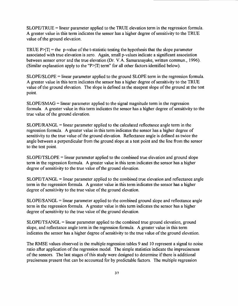
SLOPE/TRUE = linear parameter applied to the TRUE elevation term in the regression formula. A greater value in this term indicates the sensor has a higher degree of sensitivity to the TRUE value of the ground elevation.
TRUE P>|T| = the p-value of the t-statistic testing the hypothesis that the slope parameter associated with true elevation is zero. Again, small p-values indicate a significant association between sensor error and the true elevation (Dr. V.A. Samaranayake, written commun., 1996). (Similar explanation apply to the "P>|T| term" for all other factors identified below).
SLOPE/SLOPE = linear parameter applied to the ground SLOPE term in the regression formula. A greater value in this term indicates the sensor has a higher degree of sensitivity to the TRUE value of the ground elevation. The slope is defined as the steepest slope of the ground at the test point.
SLOPE/SMAG = linear parameter applied to the signal magnitude term in the regression formula. A greater value in this term indicates the sensor has a higher degree of sensitivity to the true value of the ground elevation.
SLOPE/RANGL = linear parameter applied to the calculated reflectance angle term in the regression formula. A greater value in this term indicates the sensor has a higher degree of sensitivity to the true value of the ground elevation. Reflectance angle is defined as twice the angle between a perpendicular from the ground slope at a test point and the line from the sensor to the test point.
SLOPE/TSLOPE = linear parameter applied to the combined true elevation and ground slope term in the regression formula. A greater value in this term indicates the sensor has a higher degree of sensitivity to the true value of the ground elevation.
SLOPE/TANGL = linear parameter applied to the combined true elevation and reflectance angle term in the regression formula. A greater value in this term indicates the sensor has a higher degree of sensitivity to the true value of the ground elevation.
SLOPE/SANGL = linear parameter applied to the combined ground slope and reflectance angle term in the regression formula. A greater value in this term indicates the sensor has a higher degree of sensitivity to the true value of the ground elevation.
SLOPE/TSANGL = linear parameter applied to the combined true ground elevation, ground slope, and reflectance angle term in the regression formula. A greater value in this term indicates the sensor has a higher degree of sensitivity to the true value of the ground elevation.
The RMSE values observed in the multiple regression tables 9 and 10 represent a signal to noise ratio after application of the regression model. The simple statistics indicate the impreciseness of the sensors. The last stages of this study were designed to determine if there is additional preciseness present that can be accounted for by predictable factors. The multiple regression
37

tables obviously indicate that there are identifiable factors that contribute to errors. These factors are indicated by P>|T| values lower that 0.05. Many of these may not yield practical improvements to the data because their effects (slopes) are small, but in several instances, the effects represent a significant reduction in the errors. In every land cover category there is a significant correlation between the combination of factors considered and the error reported for both sensors. This is positively identified by the very low values of the Prob>|F|. In most cases the benefit is small as indicated by the relatively low value of R-Square but there are significant benefits indicated in several land cover categories that may warrant additional study for both sensors.
38
CONCLUSIONS
The original objective of this test was to report the accuracy that can be expected from the LIDAR and IFSARE sensors. This is shown in the simple statistical test in tables 1 and 2. The LIDAR test indicates its ability to detect the ground with a mean error between -1.5 and 3.4 ft and a standard deviation of 1.4 to 8.7 ft when it has a relatively unobstructed view of the surface (land cover categories of open ground, low cover, and scrub). It is apparent that LIDAR's best results would occur over open ground, but these results are not conclusive due to the small area of this category available for this test. Even if all the points available had been used in this test instead of the sampling of points, the results would probably be the same because they represent such a small area on the ground. The points that were tested in open ground indicate the capability to produce data with a standard deviation of 1.4 ft and a mean of-1.5 ft, where the view is totally unobstructed (land cover category of open ground). The LIDAR sensor demonstrated an exceptional ability to penetrate tree cover, at least while the trees were without leaves.
The IFSARE test indicates a mean accuracy of between 3.4 and 4.6 ft with a standard deviation of 7.6 to 10.5 ft for relatively unobstructed views of the ground. This sensor did not demonstrate an ability to penetrate leafless trees.
This report has shown that there are identifiable and possibly correctable patterns within some of the data that were collected and tested. The LIDAR data show evidence that they are calibrated well for all categories except open ground. Assuming that all spatially related factors have been considered, the most benefit in four of the five land cover categories used in this test would be 2 to 8 percent reduction in the sum of the squares of the errors. And even that is very tenuous at best with low probabilities of these factors being significant. The exception is in the open ground area. This area shows the LIDAR data with a possible 73 percent reduction in the sum of squares of the errors with a high degree of significance. As stated earlier in the report, the open ground results for LIDAR are not reliable because of the shortage of test points.
With IFSARE data, there is a much higher probability that error could be reduced using the results of a regression model. In the four categories where LIDAR showed little improvement, the IFSARE showed a steady 10 to 18 percent R-squared value. This shows a potential for further refinement of this technology through calibration to the spatial and signal characteristics by adjustment of the model for detected slope and reflectance angle. These two variables recurred repeatedly as the strongest influence and most probable influence in all of the land use categories for the IFSARE data. The effect was most significant in the other category of open ground. There was strong correlation with ground slope, reflectance angle, true ground elevation, and signal magnitude in open ground. The IFSARE demonstrated a consistent correlation between possible sensor error and the actual ground elevation in all categories of land use. This could point to a calibration problem with distance measurement used to calculate ground elevation as it did in LIDAR. It should also be noted that ERIM stated that there was a 5 m horizontal bias in the positions of their data points, but they did not submit new test data when given the opportunity.
39

This test has been successful in its goal of determining the level of accuracy in these systems and providing information on some possible causes of inaccuracy. It is not always clear from these tests how much of the detected error can be corrected. However, the possibility that such corrections may produce more reliable results is indicated for some ground covers. Potential benefits of additional testing for LIDAR are not strongly indicated for reduction of systematic error for any land cover category other than open ground and even that is far from certain. The IPS ARE sensor data do indicate a strong possibility of obtaining measurable accuracy improvement from knowledge that could be gained in additional testing.
This test was run with the knowledge of the true elevations, slopes, and reflectance angles that would not be known in normal operation of these sensors. Further tests would have to be conducted using values obtained only from the sensor itself to determine if corrections are possible under actual production circumstances. For instance, a model of the ground could be made from the raw sensor data and used as an indication of ground slope or signal reflectance angle. A recursive calculation using these values could be performed to modify the results of the original raw model for comparison with ground truth for purposes of calibrating the parameters in the calculation. These tests were performed with the simplest regression model with only linear relationships considered. Future tests could also be done to determine if higher order relationships would produce better corrections. There are enough data that have been unused in conducting these tests to support such additional tests. Discussions have been held on this idea and it is felt that there are possible benefits from such tests even though they were beyond the scope of this project.
All data used for this test are available from Dan Canfield or Mike Kling at Mid-Continent Mapping center. They can be contacted at 573-308-3729 or 573-308-3732. Dr. Samaranayake can be contacted through the University of Missouri at Rolla.
40

REFERENCES
ASPRS, 1990, ASPRS Accuracy Standards for Large-Scale Maps: Photogrammetric Engineering and Remote Sensing v. 56, no. 7.
Galloway, G. E., 1994, Letter from General Gerald E. Galloway, Fr., Brigadier General, U.S. Army, Dean of the Academic Board to the Honorable John Gibbons, Assistant to the President, for Science and Technology Policy dated September 6, 1994.
IFMRC, 1994, Preliminary report of the Scientific Assessment and Strategy Team, Report of the Interagency Floodplain Management Review Committee, to the Administration Floodplain Management Task Force: A Blue Print for Change Part V, Science for Floodplain Management Into the 21st Century.
USGS, 1993, USGS Digital Cartographic Data Standards, Digital Elevation Models, U.S. Geological Survey Circular 895-B.
41

ACKNOWLEDGEMENTS
Dan Cotter, Hydrologist, Risk Assessment Branch, Mitigation Division, FEMA (resigned). Mr. Cotter was the primary contact at FEMA for the MARAT project and arranged for the early funding of the MARAT project photography and ground control collection before the GATF funding was established.
Dr. Clifford W. Greve, Special Assistant for Technology, Office of the Division Chief, National Mapping Division, USGS (resigned). Dr. Greve was the National Mapping Division contact with the GATF and was instrumental in obtaining the funding for the MARAT project.
Robert Heidelbach, Physical Scientist, U.S. Army Topographic Engineering Center, CETEC- TD-TI, Team Leader within the Imagery Research Division of the Topographic Technology Laboratory. Mr. Heidelbach was the principle contact with TEC for the MARAT project. Mr. Heidelbach was a primary MARAT contact at TEC and was instrumental in planning IFSARE ground control on the Glasgow site.
John Hill, Ph.D., director Environmental Information Systems Laboratory (EISL), Houston Advanced Research Center and adjunct professor of geography at Texas A&M University. Dr. Hill was the primary MARAT contact for HARC.
Peter B. Johnson, Supervisory Electronics Engineer, U.S. Army Topographic Engineering Center, CETEC-TD-TI, Chief of the Imagery Research division of the Topographic Technology Laboratory. Mr. Johnson was the secondary contact with TEC for the MARAT project. Peter Johnson was a primary MARAT contact at TEC.
Dennis Morgan, Head, Cartography and Photogrammetry Unit, St. Louis, Missouri USACE-St.L. Mr. Morgan was the USAGE contact for the contracts to perform the collection of the Photogrammetrically collected standard data and the ground control surveys.
Dr. V. A. Samaranayake, an associate professor from the University of Missouri at Rolla. Dr. Samaranayake was the statistician for this project.
Christine York, Intelligence Officer, Remote Sensing and Aerial Reconnaissance Team, FEMA. Ms. York was the primary MARAT contact for FEMA after Mr. Cotter resigned. She is also a member of the GATF and was instrumental in obtaining funding for this project.
42
APPENDIX A: Figures Representing the Variety of Topographic Data Sets Used in Study
Several figures are presented in appendix A. These figures are helpful in visualizing the variety of topographic data sets as generated by the specific sensors used in this study.
Figure 1 is the 3- x 3-km area from the 1:24,000-scale USGS topographic map.Figure 2 is the shaded relief of the LIDAR data.Figure 3 is the land cover map used in this study. The land cover categories are:
1 Suburban2 Trees3 Scrub4 Silo5 Low cover6 Bridge7 Water8 Beached barges9 Open ground
Figure 4 is the shaded relief of the photogrammetric standard data. Figure 5 is the shaded relief of the IF S ARE data. Figure 6 is a stereopair of photographs of the Glasgow area.Figure 7 is the photomosaic of the 3,000 ft photographs used to produce the standard. Figures 8, 9, and 10 are perspective views of the test area for the standard, IFSARE, and LIDAR elevation data.
43
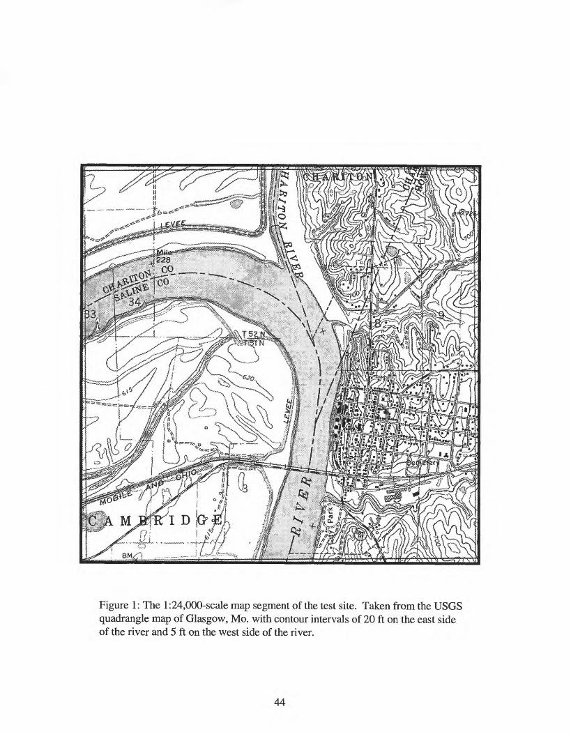
Figure 1: The l:24,000-scale map segment of the test site. Taken from the USGS quadrangle map of Glasgow, Mo. with contour intervals of 20 ft on the east side of the river and 5 ft on the west side of the river.
44
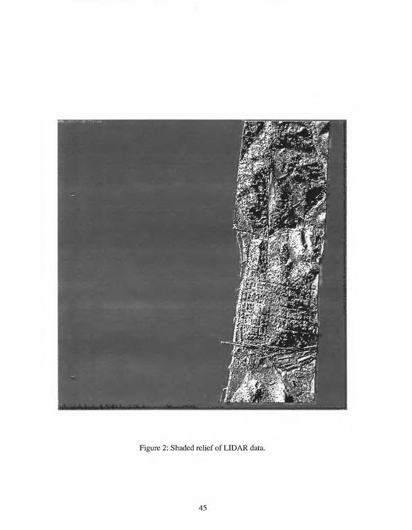
Figure 2: Shaded relief of LIDAR data.
45

Figure 3: Land cover map of test site.
46

Figure 4: Shaded relief of photogrammetric standard data.
47

Figure 5: Shaded relief of IPS ARE data.
48
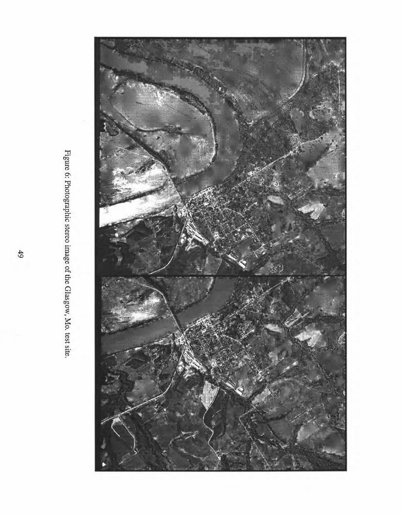
Figure 6: Photographic stereo image of the G
lasgow, M
o. test site.
49

Figure 7: Photomosaic of compilation photography
50

Figure 8: Perspective view of photogrammetric standard data.
51

Figure 9: Perspective view of IPS ARE data.
52

Figure 10: Perspective view of LIDAR data.
53
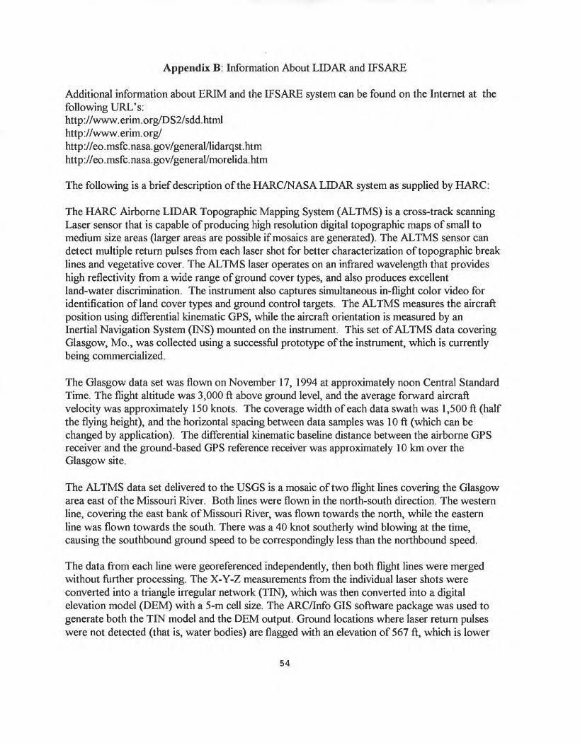
Appendix B: Information About LIDAR and IFSARE
Additional information about ERIM and the IFSARE system can be found on the Internet at thefollowing URL's:http://www.erim.org/DS2/sdd.htmlhttp ://www. erim. org/http ://eo. msfc. nasa. gov/general/lidarqst. htmhttp://eo.msfc.nasa.gov/general/morelida.htm
The following is a brief description of the HARC/NASA LIDAR system as supplied by HARC:
The HARC Airborne LIDAR Topographic Mapping System (ALTMS) is a cross-track scanning Laser sensor that is capable of producing high resolution digital topographic maps of small to medium size areas (larger areas are possible if mosaics are generated). The ALTMS sensor can detect multiple return pulses from each laser shot for better characterization of topographic break lines and vegetative cover. The ALTMS laser operates on an infrared wavelength that provides high reflectivity from a wide range of ground cover types, and also produces excellent land-water discrimination. The instrument also captures simultaneous in-flight color video for identification of land cover types and ground control targets. The ALTMS measures the aircraft position using differential kinematic GPS, while the aircraft orientation is measured by an Inertial Navigation System (INS) mounted on the instrument. This set of ALTMS data covering Glasgow, Mo., was collected using a successful prototype of the instrument, which is currently being commercialized.
The Glasgow data set was flown on November 17, 1994 at approximately noon Central Standard Time. The flight altitude was 3,000 ft above ground level, and the average forward aircraft velocity was approximately 150 knots. The coverage width of each data swath was 1,500 ft (half the flying height), and the horizontal spacing between data samples was 10 ft (which can be changed by application). The differential kinematic baseline distance between the airborne GPS receiver and the ground-based GPS reference receiver was approximately 10 km over the Glasgow site.
The ALTMS data set delivered to the USGS is a mosaic of two flight lines covering the Glasgow area east of the Missouri River. Both lines were flown in the north-south direction. The western line, covering the east bank of Missouri River, was flown towards the north, while the eastern line was flown towards the south. There was a 40 knot southerly wind blowing at the time, causing the southbound ground speed to be correspondingly less than the northbound speed.
The data from each line were georeferenced independently, then both flight lines were merged without further processing. The X-Y-Z measurements from the individual laser shots were converted into a triangle irregular network (TIN), which was then converted into a digital elevation model (DEM) with a 5-m cell size. The ARC/Info GIS software package was used to generate both the TIN model and the DEM output. Ground locations where laser return pulses were not detected (that is, water bodies) are flagged with an elevation of 567 ft, which is lower
54

than any normal elevation in the Glasgow scene. This data set includes only the first return pulse for each laser shot. The additional surface detail that is available from processing multiple return pulses was not deemed necessary for a DEM with a 5-m cell size. Non-topographic objects, such as buildings, bridges and trees, have not been removed from the final data set. Although these objects help to demonstrate the level of detail that is achievable with Lidar data, their presence may adversely influence the RMS error averages when Lidar data are compared to strictly topographic data sets.
The Glasgow data set was georeferenced using only the ground control target locations. The resulting georeferenced DEM was compared to the standard DEM data as a final accuracy check. There were three ground control targets at the north end of the mosaiced area, and three targets at the south end. Each set of three targets was arranged in an east-west line, with center target of the three appearing in the mosaic overlap region. This target arrangement produced ground reference locations at opposite edges of each flight line's ground coverage swath. The Glasgow site represents the first "out of state" flight for the LIDAR prototype and the HARC team.
The data georeference process assumes that the aircraft X, Y, and Z location, as measured by the differential kinematic GPS data, is completely accurate. The inexpensive, mechanical Inertial Navigation System currently used with the sensor, however, is subject to a slow drift in its aircraft attitude measurements. Quantitative sensor error analyses are available from HARC concerning accuracies possible by integrating a laser-ring gyroscope and filtering software into the ALTMS system. The georeference process calculates these aircraft attitude errors by comparing the measured locations of the ground control targets against the actual surveyed target locations. For the Glasgow mosaic, the INS drift along each flight line was modeled based on angular corrections measured at the north and south ends of the flight line (Dr. John Hill, written commua, 1996).
55