digital audioamplifiers: methods for high-fidelity fully...
TRANSCRIPT

Digital AudioAmplifiers: Methods for High-Fidelity Fully Digital
Class D Systems
P. T. Krein, DirectorGrainger Center for Electric Machinery
and ElectromechanicsDept. of Electrical and Computer Engineering
University of Illinois at Urbana-ChampaignC. Pascual, Z. Song, P. Midya, R. Roeckner,
D. Sarwate

Grainger Center for Electric Machines and Electromechanics University of Illinois at Urbana-Champaign
2
Preview
• “Ideal” amplifier objectives.• Vision of a fully digital amplifier.• The switching amplifier and pulse width
modulation.• Uniform vs. natural sampling.• Sampling rate and clock problems.• Upsampling.• Natural sampling conversion.• Noise shaping.

Grainger Center for Electric Machines and Electromechanics University of Illinois at Urbana-Champaign
3
Preview
• The system approach.• Some comments about sigma-delta.• “Perfecting the image” – compensation as
compared to feedback.• Results from an early prototype.• Demo.

Grainger Center for Electric Machines and Electromechanics University of Illinois at Urbana-Champaign
4
The Linear Amplifier
Digital Source
DAC
Linear
Analog Source
Linear
Poorefficiency
Noisesusceptible
Analog
Digital

Grainger Center for Electric Machines and Electromechanics University of Illinois at Urbana-Champaign
5
The Ideal Amplifier
• No power consumption from the signal.• No loss.• No distortion.• Response over the full audio bandwidth.• Able to drive arbitrary loads.

Grainger Center for Electric Machines and Electromechanics University of Illinois at Urbana-Champaign
6
The Ideal Amplifier
• No loss – requires lossless devices.• Primary choices: energy storage elements
and switches.• Most conveniently: switches connect to fixed
power supplies to deliver energy to a load without loss.

Grainger Center for Electric Machines and Electromechanics University of Illinois at Urbana-Champaign
7
Vision of a Fully Digital Amplifier
• The input signal is a digital data stream.• All processing is strictly by means of digital
computation, in real time.• The results of computation govern operation
of switches which constitute the output stage.• The switches feed the load directly – there is
no obvious analog process anywhere in the system.
• The ultimate is a digital loudspeaker.• Can this be done?

Grainger Center for Electric Machines and Electromechanics University of Illinois at Urbana-Champaign
8
The Switching Amplifier
• Since the output stage comprises switching devices connected to fixed power supplies, the only freedom is in switch timing.
• Suitable approach: pulse width modulation (PWM). But, what about fidelity?
0 1 2 3 4 5 60
0.5
1
PWM waveform and intended content

Grainger Center for Electric Machines and Electromechanics University of Illinois at Urbana-Champaign
9
The Switching Amplifier
All-Digital
Not All-Digital
DACComp Class-D
Amp
LC Low PassFilter
Switching Amplifier
Class-DAmp
LC Low PassFilter
Direct Digital Amplifier
PCM to PWM
All-Digital
Digital Speaker
Fiber Optic
Digital
Digital
Digital

Grainger Center for Electric Machines and Electromechanics University of Illinois at Urbana-Champaign
10
Equivalent Fidelity
• The need is a switched waveform in which a lossless low-pass filter can recover the signal.
• Based on bit resolution, noise plus distortion levels to maintain full fidelity:
Bits dB for LSB16 -96 dB20 -12024 -144
• PWM is known in communications to be associated with distortion.
• Can these levels be achieved?

Grainger Center for Electric Machines and Electromechanics University of Illinois at Urbana-Champaign
11
PWM Concerns
• Effects of distortion can be avoided when the switching frequency is relatively high.
• This is the usual practice in power electronics.• Based on natural sampling:
Frequency ratio In-band distortion9 -70 dB
11 -110 dB13 -154 dB15 -201 dB17 -251 dB
• Our objective becomes: how to do really precise PWM in the digital domain?
• Analog – compare piecewise-linear carrier to signal.

Grainger Center for Electric Machines and Electromechanics University of Illinois at Urbana-Champaign
12
The General PWM Process

Grainger Center for Electric Machines and Electromechanics University of Illinois at Urbana-Champaign
13
The General PWM Process
• The Fourier spectrum for a naturally-sampled PWM signal implies that a low-pass filter can indeed recover the signal.
0 5 10 15 20 25 30 35 40 45 500
0.5
1
Frequency ratio relative to signal
Rel
ativ
e co
mpo
nent
am
plitu
de
Fourier results for PWM with a switching ratio of 15:1.

Grainger Center for Electric Machines and Electromechanics University of Illinois at Urbana-Champaign
14
Uniform vs. Natural Sampling
UPWM
Comparisonwaveform
Originalanalogsignal
NPWM

Grainger Center for Electric Machines and Electromechanics University of Illinois at Urbana-Champaign
15
Sampling and Rates
• Uniform sampling generates the desired baseband signal, harmonic distortion, and switching frequency distortion.
• Natural sampling generates only the baseband signal and switching frequency distortion.
• Required step: The incoming sample stream is based on uniform samples. Compute natural samples instead.
• CD audio stream: 44.1 kHz, 16 bit.• PWM: sample value converts to widths.

Grainger Center for Electric Machines and Electromechanics University of Illinois at Urbana-Champaign
16
The PWM Clock Problem
16 bit 65536differentpossibleheights
44.1 kSa/s
16 bit 65536 differentpossible widths
2.9 GHz needed.
(Impractical)
How to overcome this problem, and still have "16-bit like" quality?
PCM PWM

Grainger Center for Electric Machines and Electromechanics University of Illinois at Urbana-Champaign
17
PWM Challenges
• Even if we could directly convert the incoming 16-bit data stream to pulse widths, there would be three problems:– The switching frequency is too low. At 44.1 kHz, a
10 kHz signal has a ratio of just 4.4:1.– The samples are uniform, so there would be
harmonic distortion in the results.– PWM clock problem. Need time resolution of 2-16
times the switching interval. Here 0.35 ns.• Now create digital processes to solve these
problems.

Grainger Center for Electric Machines and Electromechanics University of Illinois at Urbana-Champaign
18
Resolving the Problems
• Switching frequency: use upsampling to compute samples at a higher effective rate.
• Sampling: find a computational method for conversion to natural samples.
• Clock problem: use less precise time resolution and figure out how to make it work.

Grainger Center for Electric Machines and Electromechanics University of Illinois at Urbana-Champaign
19
Upsampling
• First step: perform upsampling to provide effective information content for the sample conversion process.
• Here we use a switching frequency of 8x44.1 kHz = 352.8 kHz. (Could have used 4x.)
• Upsampling is well established, and there are a few techniques available.
• Can be achieved with a digital filter, and works because the signals are bandlimited.
• Now the clock problem is worse: 43 ps.

Grainger Center for Electric Machines and Electromechanics University of Illinois at Urbana-Champaign
20
Natural Sampling Conversion
• An interpolation process.• Need relatively high order interpolation for
good results. Use Lagrange interpolation.• Four-point interpolation gives about -100 dB
worst-case distortion.

Grainger Center for Electric Machines and Electromechanics University of Illinois at Urbana-Champaign
21
Noise Shaping
• At this point we have a sequence of numbers that represent natural sampling times.
• To manage the clock problem, allow just 256 different pulse widths rather than 65536.
• With 352.8 kHz switching, the time resolution is 11 ns, and the necessary clock rate is a very reasonable 90.3 MHz. Recall that switching will be at 352.8 kHz.
• Two ways to do this:– Truncate the numbers to 8 bits.– Use a noise shaping process.

Grainger Center for Electric Machines and Electromechanics University of Illinois at Urbana-Champaign
22
Noise Shaping
• Any process we can provide generates quantization noise.
• A noise-shaping process directs this noise into a particular frequency band.
• Here a multi-bit sigma-delta modulator provides a high-pass function, and moves quantization noise into the ultrasonic range.
• The effect on waveforms resembles dithering.

Grainger Center for Electric Machines and Electromechanics University of Illinois at Urbana-Champaign
23
Noise Shaping
f (kHz)0 20 f (kHz)
Quantizationnoise
0 20
Quantizationnoise
x(n)
Quantizer
H(z) -1
u(n) y(n)
e(n)
Delta-SigmaModulator

Grainger Center for Electric Machines and Electromechanics University of Illinois at Urbana-Champaign
24
The System Approach
• At this point, the computation provides a list of switching times, with 8-bit resolution, and a master clock at 352.8 kHz for switching.
• All processing has been digital, and the switch timing is precise and constrained to clock boundaries.
• The timing values are used with counters to command the actual switch operation.

Grainger Center for Electric Machines and Electromechanics University of Illinois at Urbana-Champaign
25
The System Approach
• An important detail: the switches must operate with a break-before-make function to prevent momentary short circuits.
• This is provided by adding 32 extra clock pulses to support dead time.
• In principle, if the switches now deliver pulses to a loudspeaker, the inertia and our inability to hear high frequencies will yield only the desired signal.

Grainger Center for Electric Machines and Electromechanics University of Illinois at Urbana-Champaign
26
The System Approach
• In practice, a 352.8 kHz square wave imposed on a loudspeaker will generate significant power loss.
• A simple alternative is to provide a lossless LC filter stack between the switches and the speaker, to give the low-pass signal recovery and smooth the loudspeaker drive.
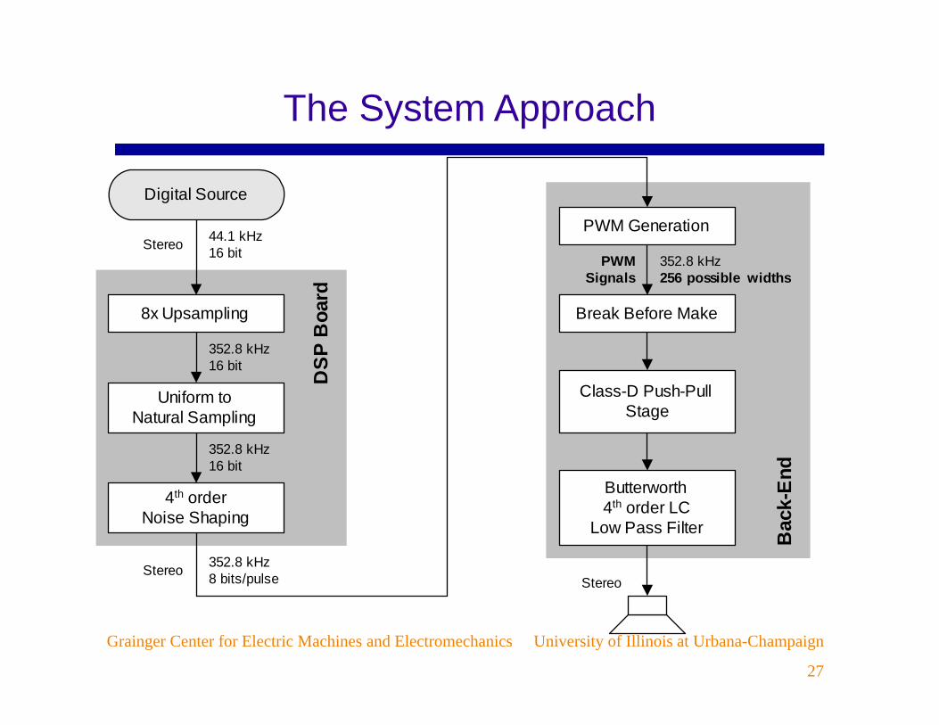
Grainger Center for Electric Machines and Electromechanics University of Illinois at Urbana-Champaign
27
The System Approach
Bac
k-E
nd
Digital Source
8x Upsampling
44.1 kHz16 bit
352.8 kHz16 bit
Uniform toNatural Sampling
4th orderNoise Shaping
352.8 kHz8 bits/pulse
Stereo
DS
P B
oard
Break Before Make
Class-D Push-PullStage
Butterworth4th order LC
Low Pass Filter
352.8 kHz16 bit
StereoStereo
PWM Generation
352.8 kHz256 possible widths
PWMSignals

Grainger Center for Electric Machines and Electromechanics University of Illinois at Urbana-Champaign
28
Power Stage and Low-Pass Filter
A
BL1 L2
C1DF
DF
TN
CX
TP
DX RX
VEXC
VSUP
B
AL1L2
C1 DF
DF
TN
CX
TP
DXRX
VEXC
C2 / 2
Speaker
MD2MD1
IN
A
B
BreakBeforeMake

Grainger Center for Electric Machines and Electromechanics University of Illinois at Urbana-Champaign
29
Comments about Sigma-Delta
• There are many publications about 1-bit sigma-delta modulators for class-D audio.
• The switching rate is linked to the “oversampling” level.
• Claim is made that sigma-delta has the advantage of noise shaping compared to PWM.
• We have seen instead that noise shaping is a separate process to be added.

Grainger Center for Electric Machines and Electromechanics University of Illinois at Urbana-Champaign
30
Comments about Sigma-Delta
• Typical example from a 2005 paper (Fujimoto, Lo Re, Miyamoto, IEEE J. SSC) uses 128x oversampling to reach 111 dB signal-to-noise ratio for 1 kHz modulation – at essentially 0 output power.
• This uses 5 to 10 times as much switching and gives much worse SNR than PWM.
• The result appears to be general: for a given power loss level and given target distortion level, PWM improves over 1-bit sigma-delta methods by a wide margin.

Grainger Center for Electric Machines and Electromechanics University of Illinois at Urbana-Champaign
31
Comments about Sigma-Delta
• Not surprising, since this system in effect can be thought of as related to an 8-bit sigma-delta modulator
• Conventional sigma-delta modulators apply uniform sampling, but with natural sampling.
• Other publications list THD+N for 1 kHz input, an easy case for PWM. (Estimated SNR for this modulation is about 160 dB.)
• We use worst-case 6.7 kHz input instead (about 60 dB higher THD+N).

Grainger Center for Electric Machines and Electromechanics University of Illinois at Urbana-Champaign
32
“Perfecting the Image”
• It is tempting to use output feedback to improve the results.
• But the bandwidth is inherently high – why risk distortion or other effects?
• Instead, a compensation approach is a good alternative.
• Are the switching edges computed by the process the same (with only delay) as those achieved?
• In other words, does the system meet its open-loop objectives?

Grainger Center for Electric Machines and Electromechanics University of Illinois at Urbana-Champaign
33
“Perfecting the Image”
• Two different approaches are possible• The first involves edge detection.
– Provide a discrete signal from the output that merely detects when edges were observed.
– Make adjustments of a bit or two in the natural sample computation to correct for any errors.
– In effect, this provides a digital feedback process, but can be slow.
• The second involves an integrator.– Confirm that the delivered energy, represented in
terms of volt-seconds, matches the command.– Make a few bits of adjustment to compensate.

Grainger Center for Electric Machines and Electromechanics University of Illinois at Urbana-Champaign
34
Laboratory Results
Uncompensated power stage Input signal Level Output power Efficiency SFDR THD+N >
6.66 kHz sinusoid -1 dBFS 55.0 W 88.0% 53 dB 0.22%
“ 0 dBFS 68.9 W 89.0% 54 dB 0.20%
“ 0 dBFS 84.1 W 87.6% 48 dB 0.40%
“ 0 dBFS 90.1 W 87.1% 45 dB 0.56%
Compensated power stage Input signal Level Output power Efficiency SFDR THD+N >
6.66 kHz sinusoid -1 dBFS 50.6 W 81.7% 73 dB 0.022%
“ 0 dBFS 63.8 W 83.4% 65 dB 0.056%
“ -1 dBFS 51.3 W 79.7% 74 dB 0.020%
“ 0 dBFS 64.8 W 82.3% 66 dB 0.050%
“ -1 dBFS 54.4 W 79.9% 72 dB 0.025%

Grainger Center for Electric Machines and Electromechanics University of Illinois at Urbana-Champaign
35
Prototype Unit
• 15 W unit (power stage on the right).• No heat sink, surface mount parts.• Has been scaled up to about 100 W.

Grainger Center for Electric Machines and Electromechanics University of Illinois at Urbana-Champaign
36
Demo
• The fully digital unit is the basis for a Motorola OEM chip set, now in pilot production.
• The production parts yield THD+N=0.006% at full power.
• For today, we have an analog naturally-sampled PWM amplifier to demonstrate the fundamental process.
• Nominal switching frequency is 160 kHz.• Natural sampling performed with LM311
comparator.• No noise shaping or extra processes.

Grainger Center for Electric Machines and Electromechanics University of Illinois at Urbana-Champaign
37
Conclusion
• The process discussed here begins with a digital audio data stream, processes it computationally, and delivers digital timing signals to a set of switches.
• For best results, a discrete timing compensation is applied, simply to ensure that the delivered waveforms match those that were commanded.
• The results, when delivered to a loudspeaker, sound like full fidelity audio.

Grainger Center for Electric Machines and Electromechanics University of Illinois at Urbana-Champaign
38
Conclusion
• Is there anything analog here? Was there any conversion?
• The results work. This demonstrates that natural sampled PWM can provide effectively undistorted output relative to the input digital audio.
• The design acts to enforce this process as accurately as possible (given practical algorithm limits), with noise shaping added to overcome timing limitations.