diffusion, attraction and collapse - harvard school of engineering

Nonlinearity12 (1999) 1071–1098. Printed in the UK PII: S0951-7715(99)02399-3

Diffusion, attraction and collapse

Michael P Brenner†, Peter Constantin‡, Leo P Kadanoff‡, Alain Schenkel‡and Shankar C Venkataramani‡§† Department of Mathematics, Massachusetts Institute of Technology, Cambridge, MA 02139,USA‡ Department of Mathematics, University of Chicago, 5734 University Avenue, Chicago,IL 60637, USA

E-mail: [email protected]

Received 5 March 1999Recommended by A Kupiainen

Abstract. We study a parabolic-elliptic system of partial differential equations that arises inmodelling the overdamped gravitational interaction of a cloud of particles or chemotaxis in bacteria.The system has a rich dynamics and the possible behaviours of the solutions include convergenceto time-independent solutions and the formation of finite-time singularities. Our goal is to describethe different kinds of solutions that lead to these outcomes. We restrict our attention to radialsolutions and find that the behaviour of the system depends strongly on the space dimensiond.For 2< d < 10 there are two stable blowup modalities (self-similar and Burgers-like) and onestable steady state. On unbounded domains, there exists a one-parameter family of unstable steadysolutions and a countable number of unstable blowup behaviours. We document connectionsbetween one unstable blowup behaviour and both a stable steady state and a stable blowup, aswell as connections between one unstable blowup and two different stable blowups. There isa topological and stability correspondence between the various asymptotic behaviours and thissuggests the possibility of constructing a global phase portrait for the system that treats the globalin time solutions and the blowing up solutions on an equal footing.

AMS classification scheme numbers: 35K55, 35B05, 58G11, 58G40

1. Introduction

In this paper we consider solutions of the parabolic-elliptic system

∂tρ = 1ρ −∇ · (ρ∇c)−1c = ρ. (1)

The scalar functionsρ = ρ(x, t) andc = c(x, t) depend onx ∈ � ⊆ Rd and ont > 0. We areinterested in solving the system (1) for domains� that are bounded as well as when� = Rd(‘the unbounded case’). For the solutions on a bounded domain, the boundary conditionsare zero flux of the scalarρ through∂� and the scalarc is zero on∂�. For solutions onRd , the boundary conditions are decay at infinity inρ and inc. These equations constitute asimplification of the Keller–Segel model [1] that was introduced in the context of chemotacticaggregation. In this interpretation,ρ represents the density of the bacteria andc representsthe density of the chemo-attractant. These equations can also be interpreted as an overdampedversion of the Chandrasekhar equation for the gravitational equilibrium of isothermal stars [2]

§ Author to whom correspondence should be sent.

0951-7715/99/041071+28$19.50 © 1999 IOP Publishing Ltd and LMS Publishing Ltd 1071

1072 M P Brenner et al

0.0 2.0 4.0 6.0 8.0 10.0r

0.0

0.5

1.0

1.5

ρ

t = 0.0t = 0.8t = 1.6t = 2.4t = 3.2t = 4.0

Figure 1. Simulation with spherically symmetric initial data in three dimensions. The solutiongoes to a time-independent density profile for large times.

or with the evolution of self-interacting clusters of particles in a viscous regime whereρ is themass density andc is the gravitational potential (see [3,4] and references therein).

Suppose one starts with some initial density distribution and asks: what is the final stateof the system? Figures 1–3 show numerical simulations that give three different final fates. Infigure 1, the diffusion wins and the densityρ spreads out so that the system heads for a steadystate. In figure 2, the densityρ blows up at some finite-timeT . En route to the blowup, themaximum of theρ(r, t) is always at the origin. In figure 3, the densityρ again blows up ata finite-timeT , but, in this case, the solution corresponds to an imploding shock and prior tothe blowup, the location of the maximum ofρ(r, t) is always off the origin. We wish to studythese and the other possible dynamical outcomes.

The problem has several experimental realizations. As was discussed above, theequations represent the dissipative dynamics of a mass densityρ interacting with itself viathe gravitational potential. In this example, blowup corresponds to gravitational collapse atlow Reynolds numbers. The time dynamics of gravitational collapse into black holes is atopic of current interest [5]. Another realization occurs in bacterial chemotaxis—the bacteriadrift up the gradient of the attractantc. This last example has recently been realized withE. Coli [6, 7]. In this context, blowup corresponds to the formation of dense aggregates ofbacteria. The experiments show a competition between cylindrically symmetric collapse (inwhich the final state is a line) and spherically symmetric clumping to a geometrical point.

From the mathematical side, the problem is one of a class of blowup problems [8] in whichsmall scales are produced in a finite time. An equation with finite-time blowup that has beenthe subject of much study is the nonlinear Schrodinger equation [9]. The blowup in the system(1) bears some similarities to the blowup in the nonlinear Schrodinger equation, both in thescaling of the self-similar blowing up solutions and in the dependence of the blowup on thedimensionality of the space. A canonical example for finite-time blowup in a parabolic PDEis the finite-time blowup in the solutions of the semi-linear heat equation

∂tρ = 1ρ + ρ2.

This problem has been studied extensively by many authors (see [10–13] and referencestherein). All the possible blowup profiles for this equation have been classified [12] and

Diffusion, attraction and collapse 1073

10−8

10−6

10−4

10−2

100

102

r10

0

102

104

106

108

1010

ρ

T−t = 8.6e−2T−t = 8.2e−3T−t = 2.8e−4T−t = 6.0e−6T−t = 9.2e−8T−t = 1.2e−9

Figure 2. Simulation with spherically symmetric initial data in three dimensions. The figure showsa log–log plot of blowup at the origin at a finite-timeT . The maximum density increases rapidlywith time signalling the onset of a singularity.

0 2 4 6 8r

0

2

4

0.00566 0.00567 0.00568 0.00569 0.0057 0.00571 0.00572r

0

1e+11

2e+11

3e+11

ρ

ρ0(r)

R(t)

δ(t)Q(t)

Figure 3. The density profile with spherically symmetric initial data in three dimensions at timeto blowupT − t = 7.13× 10−9 for the initial condition shown in the upper right corner.

recent work [13] significantly extends the scope of the analysis. The equation for the densityρ in (1) can be rewritten as

∂tρ = 1ρ −∇c · ∇ρ + ρ2,

so that these equations are similar to the semi-linear heat equations except for the presence ofthe advection term∇c · ∇ρ. It turns out that the presence of this term significantly changesthe properties of the solutions. Unlike the semi-linear heat equation, the mechanism for theblowup in system (1) depends on the space dimensiond. In the semi-linear heat equationblowup is self-similar; for the system in (1), in addition to one stable and many unstable self-


similar blowup profiles, there exists another, stable, qualitatively different blowup modality:a collapsing Burgers-like shock [14] (see figure 3). The system is rich: two different stableblowup regimes and countable many unstable ones coexist with stable and unstable steadystates.

Blowup of solutions of the Keller–Segel equations as predicted by Nanjudiah [15] andanalysed in a definitive paper of Childress and Percus [16]. The question of blowup in theKeller–Segel equations and the closely related problem of blowup in the system (1) has beenstudied by many authors (see [14, 17–26] and references therein). In this paper, we restrictourselves to the investigation of radial solutions of the system (1) inRd as well as boundedspherical domains inRd for d > 2. It is known thatd = 2 is the critical dimension for thissystem, that is finite-time singularities in the solutions of (1) can occur ford > 2 but all thesolutions are regular ford = 1 [20].

The goal of this paper is to understand the different kinds of (radial) solutions of thesystem (1). It is well known that adissipativesystem (a dynamical system with a closed andbounded absorbing set) with a Lyapunov functional, has solutions that exist for all time, andthe dynamical behaviour is characterized by a global attractor that is formed by the steadysolutions and their unstable manifolds [27,28]. The existence of a Lyapunov functional rulesout the possibility of periodic or chaotic solutions. Knowing all the steady solutions and theirrespective stabilities will enable the construction of a global phases portrait for the system thatwill describe the qualitative features of all the solutions (trajectories) of the system.

The system in (1) has an energy functional (see also [24–26]) that is non-increasing onsolutions. Unlike the dynamical systems mentioned above, this system is not dissipative;moreover it has both global (in time) solutions, and solutions with finite-time singularities.We will present evidence that it might still be possible to construct a global phase portrait ofthe system, and in this phase portrait the singular behaviour (blowup) and the non-singularbehaviour (convergence to steady states) are treated on an equal footing. To study the questionof whether it is indeed possible to construct a global phase portrait, we will analyse the varioussolutions for this system and their stability.

1.1. Summary of results

In this paper, we restrict ourselves to the analysis of radial solutions. For radial solutions, it isuseful to define a quantityh(r, t) (also see equations (7) and (11) below) by

h(r, t) = 1

2rd−2

∫ r

0ρ(r, t)rd−1 dr.

For the 2< d < 10 the results that emerge from a combination of numerical (N) and rigorous(R) analyses are summarized below.

For both bounded and unbounded domains, there are three kinds of eventual behaviourthat are stable (seen numerically without any tuning of parameters):

(i) Blowup at timeT with h(η, t) converging to a self-similar profileH0(η) ast → T − wherethe similarity variableη = r/√T − t . (R, N, see section 4.1 and also [23].)

(ii) Blowup at timeT like a Burgers shockS. This solution is not self-similar—there are twodistinct length scales in the solutionR(t) ∼ (T − t)1/d andδ(t) ∼ (T − t)1−1/d . (N, seesection 4.2 and also [14]).

(iii) Steady solutions—in an unbounded domain, the only stable steady solution isρ = 0. Adecaying solution on an unbounded domain converges to zero uniformly on compact setsin bothρ andh. In a bounded domain, if the total mass is sufficiently small, there existsa unique stable steady stateh0(r) (that depends on the total mass). (R, N, see section 3).


The blowup modalities in items (i) and (ii) are stable in the sense that the profilesH0 andS are numerically observed without any tuning of parameters. Of course, blowup solutionsare unstable, that is, a small perturbation of the initial condition, unless it is carefully tuned,may lead to a change of the blowup timeT , so that the difference between the perturbed andthe unperturbed solution can grow without bound.

Besides the stable behaviours, the following asymptotic (that is ast → ∞ for globalsolutions andt → T − for solutions that blow up atT ) behaviours of solutions are shown toexist:

(i) A countable family{Hn}, n = 0, 1, . . . of self-similar blowup modalities.H0 gives astable blowup profile. In similarity coordinates, the profile given byHn has one unstablemode corresponding to a change in blowup time and at leastn additional unstable modes.(R, see sections 4.1 and 5.1.)

(ii) A self-similar blowup modalityH∗. It is numerically seen that this blowup modality hasone unstable mode corresponding to the blowup time and one additional unstable mode.(N, see sections 4.1 and 5.1.)

(iii) Steady solutions—on an unbounded domain, there exist a one-parameter family of steadysolutions, parametrized byρ0, the density at the origin, that haveh(r)→ 1 asr →∞ thathave an infinite number of unstable directions and one neutral direction. These solutionsare monotone inρ but have an infinite number of oscillations inh. (R, N, see section 3).Taking the pointwise limit ofρ(r) or h(r) asρ0→∞, we obtain a steady solution witha singular density (see equation (18)). Taking the limitρ0→ 0 yields the steady solutionρ(r) = 0.In a bounded domain, the number of steady solutions is a function of the numberµ = h(R),whereh is as defined above andR is the radius of the domain. There existN = N(µ)steady solutionsh0, h1, . . . , hN−1. The solutionhk hask unstable directions. The solutionh0, if it exists, is the stable steady state discussed above. (R, see section 3.)

Numerical results suggest that the codimension-one unstable asymptotic behaviours (thesolutions with one unstable direction, beside the change in blowup timeT ) determine theseparatrices between the ‘basins of attractions’ of the various stable asymptotic behaviours.We find that each codimension-one solution has connections with a pair of stable solutions andthat an initial conditions lying on the boundary between the basins of attractions of differentstable behaviours will converge to a codimension-one solution asymptotically (see section 6.1).The following connections are observed numerically:

(i) The self-similar blowup modalityH1 has connections to the stable steady stateh0 and tothe stable self-similar blowupH0.

(ii) The self-similar blowup modalityH∗ has connections with the self-similar blowupH0 andwith the Burger-type shockS.

(iii) The steady solutionh1 has connections with the self-similar blowupH0 and the stablesteady stateh0.

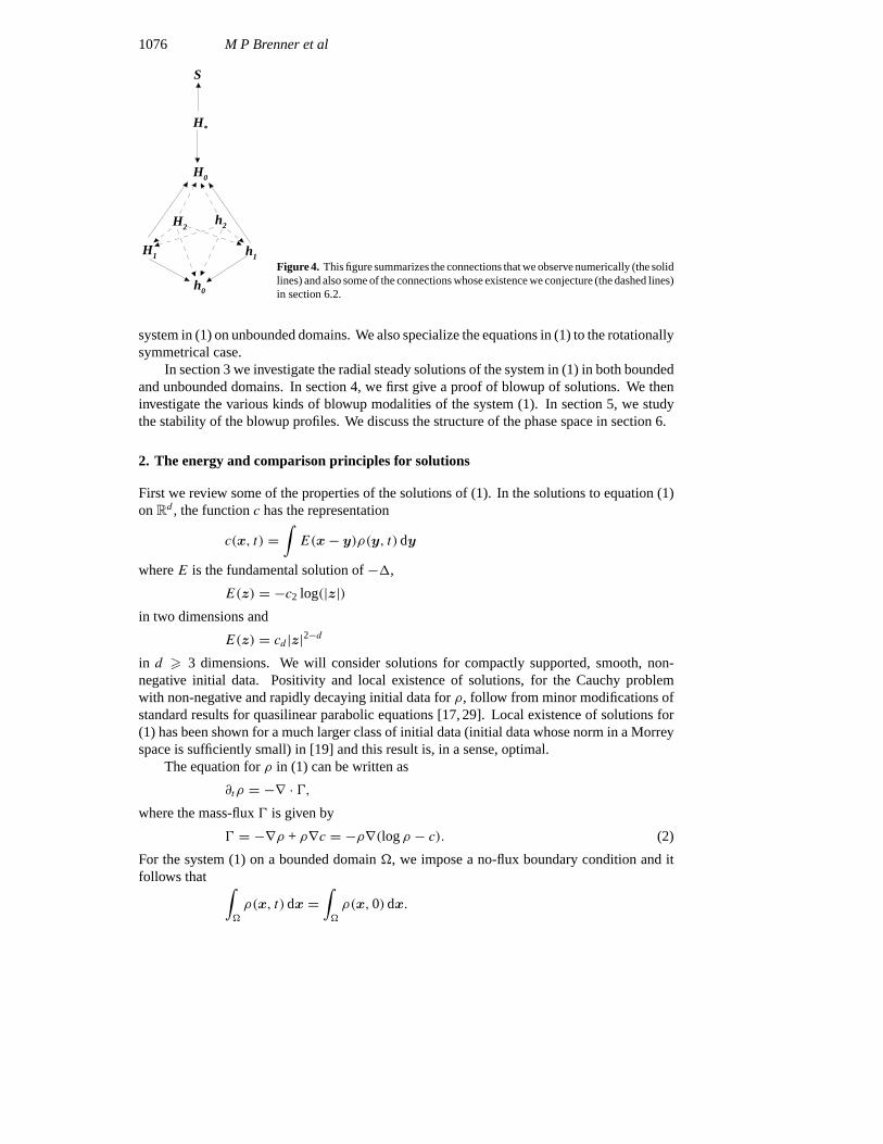
Figure 4 summarizes these numerical results for the connections between the codimension-one behaviours and the stable behaviours. It also presents our conjectures about the existenceof connections between the codimension-two behaviours and the more stable (codimensionone and codimension zero) asymptotic behaviours (see section 6.2).

1.2. Outline of the paper

This paper is organized as follows. In section 2 we collect some of the well known propertiesof solutions of the system in (1). We then describe the existence of an energy functional for the


S

H*

H0

H2h2

H1 h1

h0

Figure 4. This figure summarizes the connections that we observe numerically (the solidlines) and also some of the connections whose existence we conjecture (the dashed lines)in section 6.2.

system in (1) on unbounded domains. We also specialize the equations in (1) to the rotationallysymmetrical case.

In section 3 we investigate the radial steady solutions of the system in (1) in both boundedand unbounded domains. In section 4, we first give a proof of blowup of solutions. We theninvestigate the various kinds of blowup modalities of the system (1). In section 5, we studythe stability of the blowup profiles. We discuss the structure of the phase space in section 6.

2. The energy and comparison principles for solutions

First we review some of the properties of the solutions of (1). In the solutions to equation (1)onRd , the functionc has the representation

c(x, t) =∫E(x− y)ρ(y, t)dy

whereE is the fundamental solution of−1,

E(z) = −c2 log(|z|)in two dimensions and

E(z) = cd |z|2−din d > 3 dimensions. We will consider solutions for compactly supported, smooth, non-negative initial data. Positivity and local existence of solutions, for the Cauchy problemwith non-negative and rapidly decaying initial data forρ, follow from minor modifications ofstandard results for quasilinear parabolic equations [17, 29]. Local existence of solutions for(1) has been shown for a much larger class of initial data (initial data whose norm in a Morreyspace is sufficiently small) in [19] and this result is, in a sense, optimal.

The equation forρ in (1) can be written as

∂tρ = −∇ · 0,where the mass-flux0 is given by

0 = −∇ρ + ρ∇c = −ρ∇(logρ − c). (2)

For the system (1) on a bounded domain�, we impose a no-flux boundary condition and itfollows that ∫

�

ρ(x, t)dx =∫�

ρ(x, 0) dx.


We denote this conserved quantity by

M = M[ρ] =∫�

ρ(x) dx.

Another property of the equations is scale invariance—on unbounded domains, ifρ(x, t) is asolution then, for anyL > 0,

ρL(x, t) = L−2ρ

(x

L,t

L2

)(3)

is again a solution. To investigate the regularity of the solutions, we look at the evolution oftheLp norm ofρ(r, t). From equation (1) we obtain

d

dt

∫ρp(x, t)dx = −p(p − 1)

∫|∇ρ(x, t)|2ρ(x, t)p−2 dx + (p − 1)

∫ρ(x, t)p+1. (4)

At p = d2 the growth term in the rhs can be bound in terms of the dissipation term by∫

ρd+2

2 (x, t)dx 6 C(∫|∇ρ(x, t)|2ρ(x, t) d−4

2 dx

)(∫ρ

d2 (x, t)dx

)2/d

.

This inequality follows from the Sobolev inequality (cf Evans and Gariepy [32]) bystraightforward interpolation (or Holder inequality). This is a modification of a similar estimatefor the Keller–Segel system obtained in [17]. A consequence of this is the fact that if the initialL

d2 norm ofρ is small then it is non-increasing in time; higher norms can be shown to also

decay. This proves the regularity of solutions for initial data whoseLd2 norm is sufficiently

small. It is also known that if any of theLp norms ofρ diverge, then all the norms forp > d/2diverge simultaneously [4].

2.1. The energy in unbounded domains

Consider the quantity

E(ρ) =∫((ρ(x) log(ρ(x))− ρ(x))− 1

2ρ(x)c(x)) dx. (5)

Note that in more than two dimensions the integral ofρc is positive and always∫ρc dx =

∫ ∫E(x− y)ρ(x)ρ(y) dxdy.

The quantityE(ρ(·, t)) decays on solutions

d

dt

∫ (ρ(logρ − 1)− 1

2ρc

)dx = −

∫ρ|∇(logρ − c)|2 dx = −

∫02

ρdx.

Therefore, the energy dissipation vanishes only if the mass-flux0 = 0, so thatρ is a steady(time-independent) solution. Similar Lyapunov functionals have been used in the analysisof the system in (1) as well as the Keller–Segel system, on bounded as well as unboundeddomains, in [24–26]. The existence of a Lyapunov functional implies that (1) does not haveany periodic solutions withE finite. Therefore, every solution of (1) with a finite energy that isglobal in time has to converge to a steady (time-independent) solution. Another possibility isfor the solution to have a finite-time singularity so that the solution cannot be extended beyondthe blowup time.

Note that the functional derivative ofE isδEδρ= logρ − c


so the equation takes the form

∂tρ = ∇ ·(ρ∇ δE

δρ

). (6)

The energy can be used to deduce information about steady states. If the energy and energydissipation are well defined then the latter must vanish for time-independent solutions. In thewhole space the implications are the following: ifρ is the density of a smooth steady state andif it is strictly positive in an unbounded open connected set then it follows that logρ − c is aconstant in the same set. This implies thatρ = k exp(c) and becausec vanishes at infinityit follows thatρ does not. This is impossible if the energy is finite, so the assumptions areinconsistent: there are no steady states with a finite energy on an unbounded domain.

2.2. Radial equations

Henceforth, we restrict ourselves to solutions with spherical symmetry and treat the spacedimensiond as a parameter in the equation. Letm(r, t) be given by

m(r, t) =∫ r

0ρ(r, t)rd−1 dr, (7)

so thatm(r) is the mass inside a sphere of radiusr divided byCd = dπd/2/0((d + 2)/2) (the‘surface area’ of the unit sphere ind dimensions). From the system in equation (1), we candeduce thatm(r, t) satisfies

∂tm = ∂2r m−

d − 1

r∂rm + ρm. (8)

Under a scale transformationr → r/L, t → t/L2, the transformation of the quantitym isgiven by

mL(r, t) = Ld−2m

(r

L,t

L2

)In the variableρ, we have the integro-differential equation

∂tρ = ∂2r ρ +

d − 1

r∂rρ +

1

rd−1∂r(mρ). (9)

The boundary conditions areρ decaying at infinity for unbounded domains and zero mass fluxat the boundaries for bounded domains.

All the numerical results we present in this paper are for solutions on bounded domains.We use (9) along with the definition ofm in (7) and the no-flux boundary conditions forour numerical simulations. All the simulations were performed using a mass conserving,second order in time step, implicit scheme along with adaptive mesh refinement. Some ofthe numerical results reported in this paper were obtained with numerical routines that weredeveloped using BuGS [30], a general purpose toolkit for solving parabolic PDEs.

We define the quantitiesb(r) andh(r) by

b(r) = dm(r)

rd, (10)

and

h(r) = m(r)

2rd−2. (11)

Under a scale transformation,b transforms asρ, i.e.,

bL(r, t) = 1

L2b

(r

L,t

L2

),


andh transforms as

hL(r, t) = h(r

L,t

L2

)so thath does not pick up any powers ofL under a scale transformation. The variablesb

andh turn out to be the most convenient variables to analyse this system.b(r, t) satisfies theequation

∂tb(r, t) = 1d+2b(r, t) + ρb(r, t) = ∂2r b(r, t) +

(d + 1

r+rb(r, t)

d

)∂rb(r, t) + b2(r, t), (12)

where

1d+2 = ∂2r +

d + 1

r∂r

is the (d + 2)-dimensional radial Laplacian.h(r, t) satisfies the equation

∂th(r, t) = ∂2r h(r, t) +

(d − 3 + 2h(r, t)

r

)∂rh(r, t) +

2(d − 2)h(r, t)

r2(h(r, t)− 1). (13)

2.3. Comparison principles for radial solutions

As a consequence of the maximum principle for parabolic equations [31], we obtain thefollowing comparison principles for the radial solutions of (1):

(i) The number of oscillations of the densityρ(r, t) (the number of changes of sign inρr(r, t))is non-increasing in time.

(ii) The number of changes of sign ofh1(r, t) − h2(r, t) is non-increasing for any pair ofnon-negative solutionsh1(r, t) andh2(r, t).

These results are obtained by adapting the proofs for similar results in [29]. A consequenceof (ii) is the following.

Let m1(r, t) andm2(r, t) be solutions to equations (7) and (8) on a domain�. Ifm(r, t0) 6 mS(r, t0) holds at some timet0 for all r ∈ � thenm(r, t) 6 mS(r, t) for allt > t0.

3. Time-independent solutions

We will now investigate the steady (time-independent) solutions of equation (8). The steadysolutionsm(r) are given by

rd−1

(m′

rd−1

)′+ ρm = 0 (14)

Using equation (7), the above equation can be written as the following system of coupledODEs

ρ ′ = − ρmrd−1

, m′ = ρrd−1. (15)

The steady states are solutions to the ODEs with the initial conditions

ρ(0) = ρ0, limr→0

dm(r)

rd= ρ0. (16)

The solutions to these ODEs give us a one-parameter family of steady solutionsparametrized by the density at the originρ0. These solutions are related to each other bythe scale transformation

r → r/L, ρL(r) = L−2ρ(r/L).

Consequently, we can obtain all the steady solutions by integrating the system of equations in(15) withρ0 = 1 and rescaling appropriately.


3.1. Steady solutions ind > 2

Let mS(r) be the solution of equation (14) for a particular value ofρ0. Then we have thefollowing theorem.

Theorem 1. For d > 2, we have

hS(r) = mS(r)

2rd−2→ 1 as r →∞.

Further, for2< d < 10, the solutionhS(r) has a countable number of oscillations about theasymptotic value ofh = 1 and ford > 10, the solution is monotonic on(0,∞).

This result is obtained by doing a phase-plane analysis of the autonomous system that isobtained forh in the variablez = log(r) (see [18]).

Since all steady solutions are related by scale transformations, the one-parameter family ofsteady solutions is given byhL(r) = hS(r/L), wherehS is the particular steady solution fromabove andL is a continuous parameter. For all these steady solutions,mL(r) is asymptoticallygiven by

mL(r) = 2rd−2, (17)

independent of the initial densityρ0. Therefore, there are no finite-mass steady state solutionsfor d > 2 on an unbounded domain. There are, however, finite-mass steady solutions onbounded domains. Figure 5 shows a plot ofhS as a function ofr for d = 3. The density at theorigin isρ0 = 20.

Taking the limitL→ 0,hS(r/L) converges pointwise to the solutionh(r) = 1. This is asteady solution that corresponds to a singular density of the form

ρ(r) = 2(d − 2)r−2 (18)

and is called the Chandrasekhar solution [19]. Taking the limitL→∞, wehS(r/L) convergesto h(r) = 0 uniformly on compact sets. These limiting solutions are important in the study ofthe behaviour of solutions of (1) on unbounded domains.

We will now investigate the conditions under which there exist steady solutions in abounded domainBR (the ball with radiusR) in d dimensions with a given total massM. Wedefine the quantity

µ = h(R) = M

2CdRd−2,

10−2

10−1

100

101

102

103

r

0.0

0.5

1.0

1.5

h(r)

Figure 5. hS as a function ofr for d = 3. ρ0 = 20.


whereCd as defined above is the ‘area’ of a unit sphere ind dimensions. Since all the steadysolutions can be obtained by appropriate scale transformations of a particular steady solution(say the solutionhS(r)), it follows that there exists a steady solution inBR with a total massM if and only if we can find arµ such that

hS(rµ) = µ. (19)

For 2< d < 10, letµi represent theith extremum of the curvehS(r) with r ∈ (0,∞),i.e. not counting the point(0, 0) and letµ0 = 0. From the phase plane analysis, it is easilyseen that

µ1 > µ3 > µ5 > · · · > 1,

and

0= µ0 < µ2 < µ4 < µ6 < · · · < 1.

(See figure 5 for an illustration of these inequalities ford = 3.) Consequently, there are nosolutions to equation (19) ifµ > µ1. There is one solution forµ0 = 0 < µ < µ2, twosolutions forµ3 < µ < µ1 and so on.

Let ri denote the (i + 1)th solution to equation (19), i.e,ri is in betweenh−1S (µi) and

h−1S (µi+1). The scale factorL for obtaining the solution in the bounded domainBR is given

by

Li = R/ri.Therefore, for every solutionri of equation (19), we can find a steady solution inBR given by

hi(r) = hS( riRr).

Note thathi(r) hasi extrema in(0, R).Also note that, ifµ = 1, limi→∞ hi(r) exists pointwise, and the limiting function

corresponds to the Chandrasekhar solution (18).If M > Mc with

Mc = 2µ1CdRd−2, (20)

equation (19) has no solutions. Consequently, there exists a critical massMc such that thereexist no spherically symmetric steady solutions in a bounded domainBR with a mass largerthanMc [18]. From the above discussion, it is also clear that ifµ is such that a steady solutionexists, then the steady solution is not necessarily unique [18].

For d > 10, thehS(r) increases monotonically from 0 to 1. Therefore, there exist nosteady solutions with mass larger thanMc = 2CdRd−2 for a space dimensiond. In this casehowever, if a steady solution exists with a given mass, it is unique [18].

3.2. Stability of steady solutions in a bounded domain

As we saw above, we can have more than one steady solution with a given total mass and agiven bounded domainBR in dimensions 2< d < 10. We will now prove the following resultconcerning the stability of the various steady solutions.

Theorem 2. Let µ = M/(2Rd−2) be such that there existp steady solutionsh0(r), h1(r), . . . , hp−1(r) with the given total mass on the bounded domainBR. Then, thesolutionhi(r) that hasi extrema forr ∈ (0, R) with i > 1 is unstable and the correspondingunstable manifold has a dimensioni.


Proof. Linearizing equation (13) abouth = hi , we obtain

∂tφ(r, t) = ∂2r φ(r, t) +

(d − 3 + 2hi(r, t)

r

)∂rφ(r, t)

+2r∂rhi(r) + 2(d − 2)(2hi(r)− 1)

r2φ(r, t). (21)

We consider the eigenvalue problem for the above equation. Letφλ be a solution of

∂2r φλ(r) +

(d − 3 + 2hi(r, t)

r

)∂rφλ(r) +

[2r∂rhi(r) + 2(d − 2)(2hi(r)− 1)

r2+ λ

]φλ(r) = 0

(22)

with the initial conditions

φλ(r)→ r2 as r → 0.

We are interested in findingλn so that the solutionφλn(r) satisfiesφλn(R) = 0. If we defineψλ(r) = φλ(r)v(r), wherev(r) is given by

v(r) = exp

[1

2

∫ r

1

d − 3 + 2hi(r1)

r1dr1

],

ψλ(r) satisfies the equation

∂2r ψλ(r) + (q(r) + λ)ψλ(r) = 0

with

q(r) =[

4r∂rhi(r) + 8(d − 2)(2hi(r)− 1) + 1− (d − 2 + 2hi(r))2

r2

].

Off the origin,v(r) > 0. Therefore, the zeros ofψλ andφλ coincide off the origin. Also, ifλm > λn, by the Sturm comparison theorem,ψλm vanishes between every two zeros ofψλnand therefore it is also true thatφλm vanishes between every two zeros ofφλn . It is easily seenthat the locations of the zeros ofφλ are continuous functions ofλ.

Settingh = hi(r/L) in equation (13) withL arbitrary, yields an identity since the steadysolutions are scale invariant. Differentiating this identity w.r.t.L and settingL = 1, it iseasily seen thatf0(r) = rh′i (r) satisfies equation (22) withλ = 0 so thatφ0(r) = f0(r). Thefunctionhi(r) hasi extrema in(0, R). Therefore, the functionφ0(r) hasi zeros in the openset(0, R). By the Sturm comparison theorem and the continuity of the location of the zerosas a function ofλ, there exists aλ∗−1 < 0 such thatφλ∗−1

(R) = 0 and there are exactlyi − 1zeros forφλ∗−1

(r) in (0, R) and aλ∗0 > 0 such thatφλ∗0(R) = 0 and there are exactlyi zeros forφλ∗0(r) in (0, R).

Now, by standard results from Sturm–Liouville theory, it follows that there existλ∗−i <· · · < λ∗−2 < λ∗−1 < 0 such thatφλ∗−k (R) = 0 andφλ∗−k (r) has exactlyi − k zeros in(0, R).

All the eigenfunctions with eigenvalues less than zero are unstable.This proves ourclaim that the steady solutionhi(r) is unstable fori > 1 and the unstable manifold hasdimensioni. �

4. Blowup modalities

In the previous section, we analysed the time-independent (steady) solutions of the system (1).In this section, we will investigate time-dependent solutions with finite-time singularities. Webegin by showing that there exist spherically symmetric solutions that blowup in a finite timefor d > 2.


Theorem 3. For d > 2, there exist solutions of the radial equations (8) such that the densityblows up at a finite time, i.e., we can find sequencesrn → r∗ and tn → T ∗ < ∞ such thatlim supn→∞ ρ(rn, tn) = ∞.

Proof. For radial solutions, equation (12) gives

∂tb(r, t) = 1d+2b(r, t) + ρb(r, t), (23)

where

1d+2 = ∂2r +

d + 1

r∂r (24)

is thed + 2 dimensional radial Laplacian. Now we take a functionγ that depends on a freeparameterT

γ (r, t) = cd+2(T − t)− d+22 exp

[− r2

4(T − t)]. (25)

This function solves the backwardd + 2 dimensional heat equation with final conditionγ (·, T ) = δ. The constantcd+2 is adjusted so that∫ ∞

0γ (r, t)rd+1 dr = 1.

We note for later use that

∂rγ = − r

2(T − t)γ .

The constantT will be chosen later. Now we multiply the equation (23) byγ , integraterd+1 drand use the properties ofγ . After checking that there are no boundary contributions we obtain:

d

dt

∫ ∞0b(r, t)γ (r, t)rd+1 dr =

∫ ∞0ρ(r, t)b(r, t)γ (r, t)rd+1 dr.

We recall that

rd−1ρ = ∂rmand that

rdb(r, t)/d = m.We deduce

d

dt

∫ ∞0b(r, t)γ (r, t)rd+1 dr = 1

2d

∫ ∞0

[r2

2(T − t) + (d − 2)

]b2(r, t)γ (r, t)rd+1 dr. (26)

Now, if d > 2 we discard the first term in the square brackets and use the fact that(∫b(r)γ (r)rd+1 dr

)2

6∫b(r)2γ (r)rd+1 dr

that follows from the positivity and normalization ofγ via the Schwartz inequality. Therefore,the quantity

y(t) =∫ ∞

0b(r, t)γ (r, t)rd+1 dr

obeys the inequality

d

dty > d − 2

2dy2.


Consequently, this quantity diverges no later thant = T∞ where

T∞ = 2d

d − 2

1

y(0).

Now we will chooseT and the initial data so that

T∞ < T

and conclude that we have blowup ind > 2. Recalling that

y(0) = dcd+2

∫ ∞0T −

d+22 exp

(− r

2

4T

)m0(r)r dr,

using the definition ofm and changing the order of integration we obtain that

y(0) = 2dcd+2T− d

2

∫ ∞0ρ0(r) exp

(− r

2

4T

)rd−1 dr.

By choosing firstT > 0 and thenρ0 appropriately, for instance

ρ0(r) = Nfor r 6 T − 1

2 andρ0 = 0 for the rest we deduce thatT∞ < T follows from

Ndcd+2

∫ 1

0exp

(−x

2

4

)xd−1 dx >

1

T (d − 2),

i.e., ifNT is sufficiently large. Ifd = 2 the analysis is based on the slightly different inequality(∫ ∞0b(r, t)γ (r, t)r3 dr

)2

6 C∫ ∞

0b(r, t)2γ (r, t)

r2

2(T − t) r3 dr

with C = 4c4, but otherwise it is completely similar. �

Note that theblowup quantityy(t) is actuallya priori bounded in terms of the conservedmass. However, its time derivative is not bounded, and the argument in theorem 3 implies thatthe quantityy(t) has to develop a discontinuity (shock) before the timeT∞.

Various authors have proved the existence of solutions that blowup for the system in (1)as well as the Keller–Segel equations and other generalizations of these equations, both forradial and non-radial solutions, using a variety of techniques. Some of these proofs can befound in [17,18,20,33].

4.1. Self-similar blowup

The scale invariance (see equation (3))

r → r/L, ρL(r, t) = L−2ρ(r/L, t/L2)

motivates us to look for solutions with the parabolic scaling

L ∼ √T − t (27)

for solutions that blow up att = T . We look for solutions of the form

ρ(r, t) ∼ 1

T − t 5(

r√T − t

)(28)

subject to the boundary conditions

5(η)→ 0 as η→∞ and 5(0) <∞. (29)


10-6

10-4

10-2

100

102

104

η

0

1

2

3

H(η

)

U = -0.13071U = 0.06016U = 1.0

Figure 6. Similarity solutions for the blowup profiles ford = 3. The similarity solutions satisfylimη→∞H(η) = 1 +U . The figure shows solutions withN = 1, 2 and 3 intersections with thelineH = 1.

To look for solutions that blow up, we rewrite the equations in terms of the scaled radialcoordinateη = r/√T − t and the slow timeτ = − log(T − t), and we obtain

∂τ5 = ∂2η5 +

d − 1

η∂η5 +

1

ηd−1∂η(m(η)5)−5− 1

2η∂η5, (30)

wherem(η) = ∫ η0 ξd−15(ξ) dξ .It is again convenient to solve for the functionh(r, t) instead ofρ(r, t). Taking

note of the rescaling properties ofh(r, t), we write h(r, t) = H(η, τ). We imagine thatH(η, τ) = HS(η)+HC(η, τ ), whereHS(η) is a self-similar solution that describes the blowupandHC(η, τ ) describes the approach to the self-similar solution, so thatHC(η0, τ ) → 0 asτ →∞ for any fixedη0 <∞. In the rescaled coordinates, we can rewrite equation (13) as

∂τH(η, τ ) = ∂2ηH(η, τ ) +

(d − 3 + 2H(η, τ)

η

)∂ηH(η, τ )

+2(d − 2)H(η, τ )

η2(H(η, τ )− 1)− η

2∂ηH(η, τ ). (31)

Theτ -independent solutions of this equation that satisfy the boundary conditions

η∂ηHS(η)→ 0 as η→∞ and limη→0

HS(η)

η2<∞,

give exactly self-similar solutions that blowup at a finite-timeT . If we set∂τHS(η) = 0 in(31), we obtain

∂2ηHS +

[d − 3 + 2HS

η− η

2

]∂ηHS +

2(d − 2)(HS − 1)HSη2

= 0. (32)

Besides satisfying the boundary conditions at infinity and atη = 0, in order to describe theblowup of a solution whose initial condition is a non-negative density, we need that the solutionHS should have a non-negative density and a non-negative mass for allη > 0, i.e.,HS > 0and∂η(ηd−2HS) > 0.

Figure 6 shows numerically obtained solutions to equation (32) that satisfy the boundaryconditions and also have a non-negative mass and density.

We have the following theorem about the solutions to equation (32).


Theorem 4. For 2< d < 10, there exist a countable number of solutions to the equation

∂2ηHS +

d − 3 + 2HSη

∂ηHS +2(d − 2)HS

η2(HS − 1)− η

2∂ηHS = 0,

satisfying the boundary conditionsHS(η)/η2 is bounded asη→ 0andη∂ηHS → 0asη→∞and the requirementsHS(η) > 0, ∂η(ηd−2HS(η)) > 0 for all η.

These solutions are characterized by the number of intersections with the lineH = 1.More precisely, given a non-negative integerN , there exists at least oneU ∈ [−1, 1] and asolutionHN such that the solutionHN(η) intersects the lineH = 1 preciselyN + 1 times andlimη→∞H(η) = 1 +U .

This theorem can be proved using a shooting argument. The proof is obtained using thefollowing results:

(i) For anyU ∈ [−1, 1] with U 6= 0, there exists anη1(U) > 0 such that equation (32) has anon-negative solution on(η1,∞) with limη→∞H = 1 +U . This solution has5(η) > 0for η ∈ (η1,∞) (non-negative density) and is maximal in the sense thatH(η1) = 0 andif η1 > 0, any extension of the solution forη < η1 will makeH negative.

(ii) For anyU ∈ [−1, 1] with U 6= 0, the solution constructed above has a finite number ofintersections,N(U), with the lineH = 1 on the interval(η1,∞).

(iii) If η1(Ua) > 0, there is a connected neighbourhood ofUa whereN(U) is a constant. Onthis neighbourhood,η1 and the locations of the intersections depend continuously onU .

(iv) If Ua is such that no open neighbourhood ofUa has a constantN(U), it follows thatη1(Ua) = 0, H(0) = 0, 5(0) < ∞, we can choose an open neighbourhood ofUasufficiently small so thatN(U) attains only two distinct values on this neighbourhood,and these values differ by two.

(v) We can write down explicit solution withN(Ua) = 1 (Ua = 1) andN(Ub) = 0 (Ub = −1).(vi) Given any natural numberM, we can find aU sufficiently close to one such that

N(U) > M. Also,N(U) is odd forU > 0 and even forU < 1.

These results are proved in [34]. From these results, it is easily seen that, given any naturalnumberN , there exists at least one solution of (32) that satisfies the boundary conditions, andhasN intersections with the lineH = 1. In the proof, we also obtain that the solution withNintersections has preciselyN − 1 extrema forη ∈ (0,∞). As in the statement of the theorem,we will denote this solution byHN−1. These solutions give self-similar blowup modalities for(1). They have also been described in [23].

Remark 1. The theorem, as stated, guarantees the existence of a solutionHN havingN + 1intersections with the lineH = 1 for any given integerN > 0, but it does not make anyclaims on the uniqueness of such solutions. Numerical evidence suggests that the solutionHNwith U = limη→∞HN(η) − 1 ∈ [−1, 1] is unique. If, however, we relax the restriction thatU ∈ [−1, 1], it turns out that the solutions are not necessarily unique.

We will return to this point subsequently.

Remark 2. It is easily seen that, ford > 2, all the solutions to equation (32) satisfying theboundary conditions describe blowup where the density diverges at the origin but no mass isconcentrated at the origin, i.e.,

limε→0

(limt→T

m(ε, t))= 0.


0.0 2.0 4.0 6.0η = r/(T−t)

1/2

0.0

2.0

4.0

6.0

Π =

ρ(T

−t)

T−t = 8.6e−2T−t = 8.2e−3T−t = 2.8e−4T−t = 6.0e−6T−t = 9.2e−8T−t = 1.2e−9Theory

Figure 7. Blowup profile ford = 3. The solution converges in similarity variables to the theoreticalprofile given by51. The blowup timeT is estimated using the density at the origin.

For alld > 2, we can check that

H0(η) = 2η2

2(d − 2) + η2(33)

is a solution of equation (32) satisfying the boundary conditions and the non-negativityrequirements. This solution hasU = 1 andN = 1 (one intersection with the lineH = 1).

We will show below that all the stable self-similar blowup profiles should have no extremafor η ∈ (0,∞) so that they can have no more than one intersection with the lineH = 1.Therefore, all the other solutions to equation (32) for 2< d < 10, that are described intheorem 4, give blowup profiles that are unstable.

Figure 7 shows numerically obtained solutions to equation (1) with spherical symmetry ford = 3. The figure shows the density scaled by the inverse of the time to blowup as a functionof the radial coordinate rescaled by the square root of the time to blowup. This is preciselythe scaling in equation (28). The theoretical curve is given by the density corresponding to thesolutionH0(η) in equation (33), i.e.,

50(η) = 4(d − 2)(2d + η2)

[2(d − 2) + η2]2. (34)

We find that this blowup profile is stable in the sense that there is an open set of initial conditionsall of which blow up converging to this profile.

As we remarked earlier, the solutions withN = 1 are not unique if we relax the restrictionthatU ∈ [−1, 1]. Figure 8 showsH∗(η), a solution of equation (32) ford = 3 satisfyingthe boundary conditions withU = 16.378. . . . Also shown is the solutionH0(η) given by(33). Both these solutions haveN = 1 and have no extrema forη ∈ (0,∞) in contrast to thesolutionsHN(η) with N > 1 whose existence is guaranteed by theorem 4.

4.2. Non-self-similar blowup

In this section, we present numerical results about certain solutionsρ(r, t) that blowup in a non-self-similar fashion. By non-self-similar, we mean that the asymptotics of such solutions do not


10−2

10−1

100

101

102

η

0.0

5.0

10.0

15.0

20.0

H(η

)

H*(η) (U = 16.37)H1(η) (U = 1)

Figure 8. Similarity solutions ford = 3. This figure shows the solutionsH0(η) andH∗(η) thathaveN = 1.

develop on scales corresponding to the similarity variablesη = r/√T − t and5 = (T − t)ρ.They correspond to an imploding smoothed out shock wave that collapses into a Dirac mass atthe origin when the singularity is formed. Hence, unlike the self-similar solutions describedabove, a finite portion of the initial mass is driven to the origin at the blowup time. Ford = 3,those solutions have been analysed in [14] by means of matched asymptotics.

As mentioned in the previous section, the density profile51 given by the explicitsimilarity solution in (34) has been obtained numerically for several initial data with thedensity concentrated in balls around the origin or in shells close enough to the origin. On theother hand, starting with an initial condition whose mass is concentrated in a shell away fromthe origin, the numerical integration of equation (9) does not lead to this self-similar blowup,but to the formation of a peak moving towards the origin, with a height blowing up to infinityand a width shrinking to zero at a finite-timeT .

This behaviour is also stable in the sense that it has been observed for various such initialdata, so that it is expected for an open set of initial conditions. Figure 3 shows a typical profilejust prior to blowup. Furthermore, the dynamics of the heightQ(t) of the peak, its widthδ(t)and its locationR(t) depend upon the dimensiond and satisfy for several values ofd > 2, ast → T ,

Q(t) = c1(T − t)−2 d−1d , δ(t) = c2(T − t) d−1

d , R(t) = c3(T − t)1/d . (35)

See figures 9–11.Generalizing an argument from [14], a simple motivation for the power laws in

equation (35) goes as follows. We begin by assuming thatδ � R � 1 and that the peakcontains a finite and slowly changing portion of mass, namely thatm(R, t) ∼ Rd−1Qδ ∼ M.In the neighbourhood of the peak, we have∂rρ ∼ Q/δ and∂2

r ρ ∼ Q/δ2, so that the secondterm in the rhs of equation (9) becomes asymptotically irrelevant, leading to

∂tρ = ∂2r ρ +

1

rd−1∂r(mρ). (36)

We will require that the three remaining terms to be of the same size. Recalling that


10−13

10−11

10−9

10−7

10−5

10−3

10−1

T−t

100

103

106

109

1012

1015

Q(t

)

d = 2.5d = 3d = 4

Figure 9. The heightQ(t) for d = 2.5, 3 and 4. In the asymptotic regime, the best fits have slopesof value 1.203, 1.335 and 1.498 respectively, in good agreement with the theoretically predictedvalues of6

5 , 43 and 3

2 .

10−13

10−11

10−9

10−7

10−5

10−3

10−1

T−t

10−8

10−6

10−4

10−2

100

δ(t)

d = 2.5d = 3d = 4

Figure 10. The widthδ(t) for d = 2.5, 3 and 4. In the asymptotic regime, the best fits have slopesof value 0.602, 0.668 and 0.749 respectively, in good agreement with the theoretically predictedvalues of3

5 , 23 and 3

4 . Here,δ is defined as the width at half the height of the peak.

∂rm = rd−1ρ, we obtain

Qδ2 ∼ 1. (37)

With the mass conservation assumption, this leads to

δ ∼ Rd−1. (38)

Those relations, together withR � 1 imply for d > 2 that (36) is in turn asymptoticallyequivalent to

∂tρ = ∂r(∂rρ +

m

rd−1ρ). (39)

To estimateR(t), we next consider travelling wave solutions of equation (39) of the form


10−13

10−11

10−9

10−7

10−5

10−3

10−1

T−t

10−5

10−4

10−3

10−2

10−1

100

101

R(t

)

d = 2.5d = 3d = 4

Figure 11. The locationR(t) for d = 2.5, 3 and 4. In the asymptotic regime, the best fitshave slopes of value 0.399, 0.327 and 0.246 respectively, in good agreement with the theoreticallypredicted values of25 , 1

3 and 14 .

ρ(r, t) = ϕ(ξ), ξ = r − R(t). Assuming thatϕ andϕ′ decrease to zero asξ → ∞ andintegrating the equation forϕ once, yields

−Rϕ = ϕ′ + m

(ξ +R)d−1ϕ.

At ξ = 0 we haveϕ′ = 0, so that

R ∼ − M

Rd−1.

This yields the power law forR(t) in equation (35). The behaviours ofδ andQ follow fromequations (37) and (38).

4.3. Asymptotic solutions neglecting diffusion

In the previous section, we discussed solutions that lead to blowup on scales different fromthe parabolic scalingη = r/√T − t . In this section, we discuss the structure solutions thatblowup at timeT on scalesL(t)� √T − t withL(t)→ 0 ast → T , so that the density blowsup att = T but the diffusion term becomes asymptotically irrelevant. Since the nonlinearitygives∂tρ ∼ ρ2, we consider the following ansatz for solutions that blowup att = T :

ρ(r, t) = 1

T − t 5(η, τ )whereη is the similarity variabler/L(t), L(t) is an as yet unspecified function oft andτ = − log(T − t). To describe a blowup we will require that5 satisfy the boundary conditions

5(0) <∞, 5(η)→ 0 as η→∞,with 5(η) > 0 for all η > 0. As before, we shall eventually go to a similarity solution byrequiring that the solution beτ independent. Using the above ansatz, equation (10) gives

b(r, t) = 1

T − t B(η, τ )and equation (12) can be written in the form:

∂τB +B − (T − t)d logL

dtη∂ηB = T − t

L2(t)1d+2B +

B

dη∂ηB +B2, (40)


where1d+2 is the (d + 2)-dimensional Laplacian inη. UsingL(t)� √T − t , we see that thediffusive term is asymptotically irrelevant in comparison with the nonlinearity. Assuming thatwe approach aτ -independent solution forB asτ →∞, we obtain the asymptotic equation[

B

d− α

]η∂ηB = B − B2, (41)

with

α = − limt→T

(T − t)d logL

dt.

In particular, forL(t) = (T − t)β , we haveα = β andL(t) � √T − t requires thatα > 12.

The caseα = 12 occurs for example withL(t) = √(T − t)| log(T − t)| which is the scaling

for a family of solutions for the semi-linear heat equation [12].From the boundary conditions specified above, we see that the solution should satisfy

B(0) <∞ and B(η)→ 0 as η→∞.Definingξ = logη, equation (41) can be written as the autonomous system

Bξ = d B − B2

B − dα . (42)

The fixed point atB = 0 is stable, the fixed point atB = 1 is repelling, and there are nocritical points in the interval(0, 1) if α > 1/d. Consequently, for 1/d < α 6 1

2, given anyC ∈ (0, 1), we have a solution of equation (42) withB(ξ = 0) = C,

limξ→−∞

B = 1 and limξ→∞

B = 0,

so that it satisfies the boundary conditions. We therefore have a continuous family of solutionsfor eachα that satisfy the boundary conditions. We can integrate equation (42) to obtain theimplicit solutions(

1− BB

)α(1− B)−1/d = keξ = kη, (43)

wherek ∈ (0,∞) is an arbitrary constant that parametrizes the continuous family of solutions.These solutions satisfyB ≈ 1− k1η

d/(dα−1) for smallη andB ≈ k2η−1/α for largeη wherek1

andk2 are constants that depend on the parameterk.

5. Stability and convergence properties of blowup profiles

In section 4.1, we saw that the system has a countable number of possible self-similar blowupprofiles with the parabolic scaling (equation (27)). This brings up the question of which ofthese profiles are stable (that are seen if we start from arbitrary initial data).

5.1. Stability of the blowup profiles

We will now prove the following result concerning the stability of the various blowup profiles.

Theorem 5. Every self-similar solutionHS(η) that blows up at a finite time has an unstablemode corresponding to changing the blowup time. Also, a blowup profile withn extrema in(0,∞) has at leastn additional unstable modes.

Proof. Linearizing equation (31) aboutH = HS , we obtain

∂τ8(η, τ ) = ∂2η8(η, τ ) +

(d − 3 + 2HS(η)

η− η

2

)∂η8(η, τ )

+2η∂ηHS(η) + 2(d − 2)(2HS(η)− 1)

η28(η, τ). (44)


We will consider the eigenvalue problem for the above equation. For a givenλ, let8λ be asolution of

∂2η8λ(η) +

(d − 3 + 2HS(η, t)

η− η

2

)∂η8λ(η)

+

[2η∂ηHS(η) + 2(d − 2)(2HS(η)− 1)

η2+ λ

]8λ(η) = 0. (45)

Then,8λ(η)e−λτ is a solution of equation (44). Nearη = 0, the leading behaviours of thetwo linearly independent solutions of (45) are8λ(η) ∼ η2 and8λ(η) ∼ 1/ηd−2. To haveHnonsingular nearη = 0, we will require the boundary condition

8λ(η)→ η2 as η→ 0.

For largeη, the leading behaviours of the two independent solutions are8λ(η) ∼ η−(2λ+1)eη2/4

and8λ(η) ∼ η2λ. Although the functionsη2λ diverge asη→∞, in terms ofr andt , we have

η2λe−λτ = r2λ,

is bounded forr bounded ast → T . Consequently, the solutions which behave likeη2λ areadmissible but the functions that behave likeη−(1+2λ)eη

2/4 diverge at finiter as t → T andare consequently inadmissible. Therefore, we are interested in findingλn so that the solution8λn(η) also satisfies the boundary condition

8λn(η)e−η → 0 as η→∞.

We have the freedom to choose the blowup timeT , i.e.,HS(r/√T + δ − t) is a solution

to equation (13) for allδ. Usingη = r/√T − t andτ = − log(T − t), we see that, settingH(η, τ) = HS(η, τ, δ) yields an identity where

HS(η, τ, δ) = HS(r/√T + δ − t

)= HS

(η

√e−τ

e−τ + δ

).

Differentiating the resulting identity w.r.t.δ, settingδ = 0, and comparing the resultingequation with equation (45), we see thatF 0

S (η) = η∂ηHS(η) is an eigenfunction with aneigenvalueλ = −1 since it also satisfies the boundary conditionsF 0

S (η) ∼ η2 asη → 0andF 0

S (η)e−η → 0 asη → ∞. If the functionHS(η) hask extrema in(0,∞), the function

8−1(η) = F 0S (η) hask zeros in(0,∞). Now, by standard results from Sturm–Liouville theory,

it follows that there existλ∗−k < · · · < λ∗−2 < λ∗−1 < λ∗0 = −1 such that8λ∗−j (η)e−η → 0 as

η→∞ and8λ∗−k (η) has exactlyk − j zeros in(0, R).The eigenfunctions with eigenvalues less than zero are unstable. This proves our claim that

all the self-similar blowup profilesHS(η) have an unstable mode corresponding to changingthe blowup time. Further, a blowup profile withk extrema in(0,∞) has at leastk additionalunstable modes. �

This theorem implies that a self-similar blowup profile that is stable to small perturbationsin the initial conditions (except for possibly a change in the blowup time) cannot have anyextrema forη ∈ (0,∞).

5.2. Convergence to the stable blowup profile

A formal procedure for determining the stability of blowup profiles is as follows. We willassume that we are sufficiently close to the blowup so that we can use the linear equation (44)to describe the stability of the blowup profileHS(η). If we choose the blowup timeT correctlyin the definition ofτ andη, we can eliminate the mode corresponding to the change in blowuptime. From the linear analysis in the preceding section, we have

H(η, τ) = HS(η) + aF 1S (η)e

−λ1τ + O(e−λ2τ ), (46)


close to the blowup, whereλ1 andλ2 are respectively the smallest and the next to smallesteigenvalues in the set of all the eigenvalues of equation (45) excluding the eigenvalue−1. F 1

S isthe eigenfunction corresponding toλ1 anda is an constant depending on the initial conditions,generically not equal to zero.

If the blowup profile is stable to small perturbations in the initial conditions, it followsfrom equation (46) that

λ1 > 0.

Given a similarity solutionHS , we can calculateλ1 numerically from equation (44). Ford = 3andHS(η) = H0(η) = 2η2/(2(d − 2) + η2), we obtainλ1 ≈ 0.27. We also find thatλ1 > 0for H0(η) for all d > 2. Therefore, the similarity solution

H0(η) = 2η2

2(d − 2) + η2,

will be seen generically in solutions that blowup according to the parabolic scaling. Usingh(r, t) = H(η, τ) and the definition ofh, we get

ρ(r, t) = 4(d − 2)(2d(T − t) + r2)

(r2 + 2(d − 2)(T − t))2 + a(T − t)λ1

T − t 511

(r√T − t

)+ O((T − t)λ2−1), (47)

where

511(η) =

1

ηd−1∂η(2η

d−2F 11 (η)).

Using the factF 11 (η)→ η2 asη→ 0, we have

ρ(0, t) = 1

(T − t)[

2d

d − 2+ 2ad(T − t)λ1 + o((T − t)λ2)

]. (48)

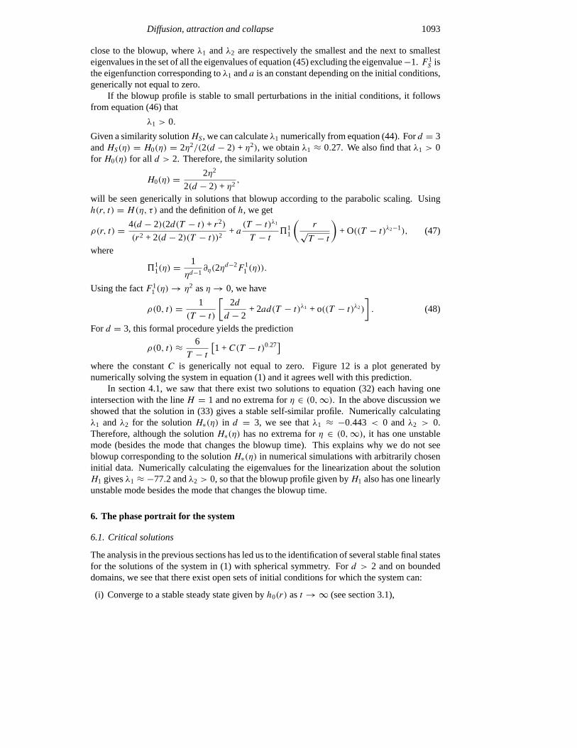
Ford = 3, this formal procedure yields the prediction

ρ(0, t) ≈ 6

T − t[1 +C(T − t)0.27

]where the constantC is generically not equal to zero. Figure 12 is a plot generated bynumerically solving the system in equation (1) and it agrees well with this prediction.

In section 4.1, we saw that there exist two solutions to equation (32) each having oneintersection with the lineH = 1 and no extrema forη ∈ (0,∞). In the above discussion weshowed that the solution in (33) gives a stable self-similar profile. Numerically calculatingλ1 andλ2 for the solutionH∗(η) in d = 3, we see thatλ1 ≈ −0.443 < 0 andλ2 > 0.Therefore, although the solutionH∗(η) has no extrema forη ∈ (0,∞), it has one unstablemode (besides the mode that changes the blowup time). This explains why we do not seeblowup corresponding to the solutionH∗(η) in numerical simulations with arbitrarily choseninitial data. Numerically calculating the eigenvalues for the linearization about the solutionH1 givesλ1 ≈ −77.2 andλ2 > 0, so that the blowup profile given byH1 also has one linearlyunstable mode besides the mode that changes the blowup time.

6. The phase portrait for the system

6.1. Critical solutions

The analysis in the previous sections has led us to the identification of several stable final statesfor the solutions of the system in (1) with spherical symmetry. Ford > 2 and on boundeddomains, we see that there exist open sets of initial conditions for which the system can:

(i) Converge to a stable steady state given byh0(r) ast →∞ (see section 3.1),


10−10

10−8

10−6

10−4

10−2

100

T−t

10−2

10−1

100

101

6−ρ(

0)(T

−t)

SimulationSlope of fit = 0.23

Figure 12. Convergence to the blowup profile. The slope of the best fit is 0.23 in good agreementwith the linear analysis which gives 0.27. Note that this exponent is small so that the convergenceis very slow and one has to solve the equations until very close to the blowup time to see theconvergence to the self-similar solution.

(ii) Blow up at a finite-timeT converging to the self-similar blowup profile given byH0(η)

in equation (33) (see section 4.1), or(iii) Blow up at a finite-timeT in a non-self-similar fashion (see section 4.2 and equation (35)).

The fate of an initial condition not only depends on its conserved total mass, but also onthe density distributionρ0(r). The existence of more than one kind of stable behaviour bringsup the question of what determines the boundaries (separatrices) between the different sets ofinitial conditions that correspond to different final states. A related question is what happensto solutions whose initial data lies on the separatrix between the basins of attraction of twodifferent types of stable behaviours.

We investigate these questions numerically by following the solutions for a family ofinitial conditionsρ0(r, p) parametrized by a parameterp. The family of initial conditions ischosen such that the final states for the initial conditions given byp = p0 andp = p1 aredifferent. In that case, there exists at least one critical valuepc ∈ (p0, p1) such that the finalstates for initial conditions for anypa andpb sufficiently close topc with pa < pc < pbare different. We find the critical valuepc by successive bisection and we can determine theseparatrix by following the solution with initial conditionρ0(r, pc) for different families ofinitial conditions.

Using this bisection method, we investigate the separatrices between the initial conditionsthat converge to the steady solutionh0, that blowup in a self-similar fashion given byH0, andthat blowup in a non-self-similar manner by an imploding shock. We find that the boundariesbetween initial conditions leading to different kinds of stable behaviour are sets of initialconditions that ‘converge’ to ‘unstable behaviours’ with one unstable direction (codimensionone asymptotic behaviours). If the relevant unstable behaviour is a steady state with oneunstable direction, then bothρ or h converge uniformly on compact sets to the appropriatelimits. On the other hand, it is also possible that the relevant behaviour is a blowup modalitythat has an unstable mode besides the mode that changes the blowup time. In this case, therescaled density5(η, τ) andH(η, τ) converge uniformly to the appropriate limits on compact


0.0 5.0 10.0 15.0 20.0r(ρmax)

1/2

0.0

0.2

0.4

0.6

0.8

1.0

ρ/ρ m

ax

Π0Π1ρmax = 4ρmax = 16ρmax = 64ρmax = 256ρmax = 1024

Figure 13. Rescaled solutions ind = 3 for an initial condition that is close to the separatrixbetween solutions converging to the steady state and self-similar blowup with a profile given byH0 (stable blowup). In this case, the relevant critical solution is the self-similar blowup given byH1.

sets in the similarity variableη asτ →∞.We will refer to the final states for initial conditions lying on the separatrix between

different basins of attraction as critical solutions. If we choose an initial conditionρ0(r, pd)

with pd close to the critical valuepc, the solution has a transient phase when it stays close tothe separatrix and seems to converge to the critical solution. However, it will eventually moveaway from the critical solution along the unstable direction and end up in one of the stablefinal states for the system.

For 2< d < 10, if the total mass is smaller than the critical massMc(R) for a domainof sizeR (see equation (20)), one possible final state is the stable steady state given byh0(r).Numerical evidence suggests that the separatrixM0 between the stable steady state and thestable self-similar blowup contains at least two pieces. One pieceMa is given the initialconditions that converge to the steady stateh1(r) that has one unstable mode. Another pieceMb is given by the set of solutions converging to the self-similar blowup profile given byH1(η),which also has one unstable direction (if we eliminate the mode that changes the blowup time).

Figure 13 shows numerically obtained solutions of equation (9) ind = 3 for an initialcondition that is very close to the separatrix between between solutions converging to thesteady state and self-similar blowup with a profile given byH0 (stable blowup). In this case,the relevant critical solution is the self-similar blowup given byH1. A linearization about thissolution gives an unstable eigenvalueλ ≈ −77.2. Since this is very large, it is difficult to obtainsolutions with a long transient phase during which the solution is close to the critical solutionH1. In this case, it is also difficult to estimate the blowup time appropriate for the solution inthe transient phase since there are solutions close to the critical solution that converge to thestable steady state and hence are global in time. Therefore, we normalize the density, using itsmaximum valueρmax , rather than the inverse of the time to blowup 1/(T − t) and the radialcoordinate byρ−1/2

max rather that√T − t . This implies that we have effectively used one-fitting

parameter to obtain the agreement of the curves in figure 13.We also investigate the separatrix between the basins of the self-similar blowup and non-

self-similar blowup. In this case, the relevant critical solution turns out to be the blowup


modalityH∗. Our solutions follow track this blowup profile until very close to the time ofblowup. They eventually diverge away from the critical solution but during this transientperiod, the density blows up on the self-similar scales and converges in the similarity variablestowards a profile which is in very good agreement with the solution5∗ corresponding to theunstable solutionH∗.

Figure 14 shows numerically obtained solutions of equation (9) ind = 3 for an initialcondition that is very close to the separatrix between the self-similar blowup and non-self-similar blowup. Since the unstable eigenvalue corresponding toH∗, λ ≈ −0.443 is not verylarge, it is possible to find initial conditions such that the solutions remain close to the criticalsolution during the interval whereρmax grows by many orders of magnitude. Also, in this case,it is possible to estimate the blowup time relevant to the transient regime by setting it equalto the blowup time of the solution. Although the solution will move away from the criticalsolution and blowup, and toward one of the stable blowup modes, the errors we make are verysmall since the solution stays close to the critical solution until about 10−22 before the blowup.The density is normalized by the inverse of the time to blow up and the radial coordinate isscaled by the square root of the time to blowup. The function5∗ is also shown for comparison.Note that the scaled density profiles eventually start to diverge away from the curve given by5∗ (for t ∼ T − 10−22).

6.2. Connections and the global phase portrait

We will first consider the case of solutions on a bounded domainBR. From the analysis ofthe structure and the stability of the various solutions, we see that there is a correspondencebetween the blowup modalityHk and the steady solutionhk. They both havek extrema andk linearly unstable modes. The solutionH∗ has one linearly unstable mode and the solutionS (the Burger-like shock) is stable. Based on the numerical results that we discuss in thepreceding section, we make the following conjectures about the structure of the phase spacefor radial solutions on a bounded domain:

0 5 10 15 20 25 30r/(T−t)

1/2

0.00

0.25

0.50

0.75

1.00

1.25

(T−

t)ρ

TheoryT−t = 5.49e−4T−t = 3.37e−5T−t = 1.29e−7T−t = 5.02e−10T−t = 1.95e−12T−t = 7.59e−15T−t = 2.96e−17T−t = 1.15e−19T−t = 1.12e−22T−t = 2.67e−23

Figure 14. Blowup profile ind = 3 for an initial condition that is close to the separatrix betweenthe self-similar blowup and the non-self-similar blowup. The blowup timeT is the blowup timefor the solution.T is very close to the blowup time of the unstable solution that it tracks in thetransient phase because the initial condition is chosen very close to the separatrix. The theoreticalcurve is the density profile for the solution5∗ and there are no parameters that are fit.


(i) The steady solutionhk and the blowup modalityHk each has connections with the 2kbehaviours{hi,Hi}, i = 0, 1, . . . , k − 1.

(ii) The behaviourH∗ has connections with the stable self-similar blowupH0 and the Burger-like shockS.

Figure 4 illustrates some of these conjectures.For the case of the unbounded domain, we no longer have the multiple steady solutions

h0, h1, . . . . Instead, we have a family of self-similar decaying solutions given byh(r, t) =H (r/√t). These solutions converge toh(r) = 0 uniformly on compact sets. The number of

these solutions is a function ofν defined byν = lim

r→∞h(r, t) = limζ→∞

H (ζ ),

and there existN = N(ν) self-similar decaying solutions given by the profilesH0(ζ ), H1(ζ ), . . . , HN−1(ζ ), with limζ→∞ Hk(ζ ) = ν for all k. It can be shown that thetransient solutionh(r, t) = Hk(r/

√t) hask extrema in(0,∞), and it hask linearly unstable

directions, so that it is analogous to the solutionhk on a bounded domain. Our conjectures forthe structure of the phase space for solutions on unbounded domains are:

(i) The behavioursHk and Hk have connections with the 2k behaviours{Hi, Hi}, i =0, 1, . . . , k − 1.

(ii) The behaviourH∗ has connections with the blowup modalityH0 and the Burger-like shockS.

7. Conclusions

We have studied a parabolic-elliptic system (1) which describes the evolution of a compressibleactive scalar that diffuses and is advected by the gradient it generates. We have discussed theexistence, stability and connections between steady solutions, parabolic self-similar blowupsolutions and Burgers like blowup solutions for this system. We find that the system hasrich dynamics with multiple steady states, multiple parabolic self-similar blowups and non-self-similar blowup. We prove results on the number of linearly unstable modes for thevarious steady solutions and the self-similar blowup profiles. Numerically, we find heteroclinicconnections between different modalities of blowup, between steady states and blowup,and most remarkably between blowup and steady states. Using these connections and thecorrespondence between the number of unstable directions of the various solutions, we beginto sketch a global phase portrait that encompasses both the smooth behaviour and the singularityformation. This task is not complete yet and we expect the situation to be rather complicated.There remain many open problems, among them the connections between the unstable steadystates and the unstable self-similar blowup profiles; the role of the solutions from section 4.3that are not self-similar with the parabolic scaling; questions about the similarities and thedifferences between the phase portraits for finite domains and for unbounded domains; andlast but not the least, proving the conjectures about the structure of the phase space.

Acknowledgments

We wish to thank Frank Merle for valuable discussions. We also wish to thank Bruce Ayati,Howard Berg, Elena Budrene, Todd Dupont, Leonid Levitov and Saleh Tanveer for many usefuldiscussions. The work of AS was supported by the Fonds National Suisse. The work of MBwas supported by the National Science Foundation (Department of Mathematical Sciences).The work of PC, LPK and SCV was supported by the MRSEC program of the National ScienceFoundation under Award Number DMR-9808595. LPK was also supported by the ONR (grantN00014-96-1-0127) and the NSF (grant DMR 9728858).


References

[1] Keller E F and Segel L A 1970J. Theor. Biol.26399–415Murray J 1989Mathematical Biology(Berlin: Springer)

[2] S Chandrasekhar 1967An Introduction to the Study of Stellar Structure(New York: Dover)[3] Wolansky G 1992Arch. Ration. Mech. Anal.119355–91

Wolansky G 1992J. Anal. Math.59251–72[4] Biler P and Nadzieja T 1994Colloq. Math.LXVI 319–34[5] Evans C R and Coleman J S 1994Phys. Rev. Lett.721782–5

Koike T, Hara T and Adachi S 1995Phys. Rev. Lett.745170–3Gundlach C 1997Phys. Rev.D 55695–713Bizon P 1996Acta Cosmol.2281(Bizon P 1996Preprinthttp://xxx.lanl.gov/abs/gr-qc/9606060)

[6] Budrene E O and Berg H C 1991Nature349630Budrene E O and Berg H C 1995Nature37649–53

[7] Brenner M P, Levitov L and Budrene E O 1998Biophys. J.741677[8] Barenblatt G I 1979Similarity, Self Similarity and Intermediate Asymptotics(New York: Consultants Bureau)[9] Landman M J, Papanicolaou G C, Sulem C and Sulem P L 1988Phys. Rev.A 383837

Malkin V M 1993PhysicaD 64251McLaughlin D W, Papanicolaou G C, Sulem C and Sulem P L 1986Phys. Rev.A 341200Luther G G, Newell A C and Maloney J V 1994PhysicaD 7459Fraiman G M 1985Sov. Phys.–JETP61228

[10] Giga Y and Kohn R V 1985Commun. Pure Appl. Math.38297–319[11] Herrero M A and Velazquez J J L1996Math. Ann.306583–623[12] Bricmont J and Kupiainen A 1994Nonlinearity7 539–75[13] Merle F and Zaag H 1998Commun. Pure Appl. Math.51139–96[14] Herrero M A, Medina E and Velazquez J J L1997Nonlinearity101739–54[15] Nanjudiah V 1973J. Theor. Biol.4263–105[16] Childress S and Percus J 1981Math. Biosci.56217–37[17] Jager W and Luckhaus S 1992Trans. Am. Math. Soc.329819–24[18] Biler P, Hilhorst D and Nadzieja T 1994Coll. Math.LXVII 297–308[19] Biler P 1995Stud. Math.114181–205[20] Nagai T 1995Adv. Math. Sci. Appl.5 581–601[21] Diaz J I and Nagai T 1995Adv. Math. Sci. Appl.5 659–80[22] Herrero M A and Velazquez J J L1996Math. Ann.306583–623[23] Herrero M A, Medina E and Velazquez J J L1997 Self-similar blow-up for a reaction-diffusion systemPreprint[24] Gajewski H and Zacharias K 1998Math. Nachr.19577–114[25] Biler P and Nadzieja T 1998Adv. Diff. Eqns3 177–97[26] Biler P 1998Adv. Math. Sci. Appl.8 715–43[27] Babin A V and Vishik M I 1992Attractors of Evolution Equations(Amsterdam: North Holland)[28] Temam R 1988Infinite-Dimensional Dynamical Systems in Mechanics and Physics(New York: Springer)[29] Samarskii A A, Galaktionov V A, Kurdyumov S P and Mikhailov A P 1995Blow-up in Quasilinear Parabolic

Equations(Berlin: de Gruyter and Co)[30] Ayati B P 1996BuGS 1.0 User Guide, Technical ReportTR–96–18[31] Protter M H and Weinberger H F 1967Maximum Principles in Differential Equations(Englewood Cliffs, NJ:

Prentice-Hall)[32] Evans L C and Gariepy R F 1992Measure Theory and Fine Properties of Functions(Boca Raton, FL: Chemical

Rubber Company)[33] Biler P and Woyczynski W A 1997 Global and exploding solutions for nonlocal quadratic evolution problems

Preprint[34] Brenner M P, Constantin P, Kadanoff L P, Schenkel A and Venkataramani S C 1998Technical Report Preprint

http://mrsec.uchicago.edu/∼scvenkat/pubs/singular.ps.gz

diffusion, attraction and collapse - harvard school of engineering

Documents