diffraction in the asymptotic solution of a dispersive hyperbolic equation

$: Diffraction in the asymptotic solution of a dispersive hyperbolic equation$
Diffraction in the Asymptotic Solution of a Dispersive Hyperbolic Equation

NORMAN BLEISTEIN

Communicated by C.C. LIN

1. Introduction

Diffraction in space-time is a feature of the asymptotic solution of dispersive hyperbolic equations. In [2] an example of this phenomenon was described for the Klein-Gordon Equation which is the simplest example of an energy preserving dispersive hyperbolic equation. It can be applied to the problem of wave propagation in a plasma [9] in which case the large parameter 2 is a plasma frequency. Here we describe a different sort of space time diffraction, again for an asymptotic solution to Klein-Gordon equation.

The name, space time diffraction, and even the very existence of this phenomenon, are suggested by the similarities in asymptotic solutions of dispersive hyperbolic equations and elliptic equations (see, for example, [8, 10, 11 ]).

In the problem studied here we consider a one dimensional dispersive medium with an interface at x = 0 . The solution u(t,x) we seek is the "Riemann function" or "radiation function" (see [4]) for the Klein-Gordon equation, i.e., we take U(0,x)=0, Ut(O,x)=6(X-Xo) with Xo<0. For t > 0 a wave is radiated toward x = - o o and another toward the interface. For dispersive equations, the "group speed" is frequency dependent [8, 9, 12] and hence each frequency component of the wave travels at a different speed. Consequently, for the wave moving toward increasing x, each component arrives at the interface at a different time. Incidence at the wall gives rise to a reflected component moving toward - oo and, in some cases, to a transmitted component, moving toward + oo. We show that there is a critical frequency for which a portion of the wave is "trapped" at the interface. This gives rise to a wave "shed" back into the region x < 0 at this critical frequency. This space-time diffracted wave continues to radiate for all time past a certain "critical time".

In Section 2, we define the problem to be studied and give an integral representation of the solution. For x < 0, this representation consists of a sum of integrals which we call Up + Us. For x > 0 we have a single integral UT.

In subsequent sections we obtain asymptotic expansions of these integrals for large values of a parameter 2 appearing in the original problem. The space-time diffracted wave arises as a part of the asymptotic expansion of Us and is obtained in Section 5.

In Section 7 we give a " ray" interpretation to the asymptotic solution. We also show that there is a boundary in space-time across which the asymptotic

Dispersive Hyperbolic Equations 215

expansion of Us, as given in Sections 4 and 5, is invalid. In Section 8 a uniformly valid asymptotic expansion of U s is obtained by a method developed by the author [1 ].

2. The Problem and Its Exact Solution

We consider the problem for U defined by the equation

(2.1) Uxx-Utt-22bZ(x)U=O, t_>__0, 2>> 1;

with

b(x)=fbb+, 1 > 0 , b+>b_ (2.2) , x < 0 ,

For initial conditions we take

(2.3) U(0, x ) = 0 , Ut(O, x)=6(X-Xo), Xo<0,

and at x = 0 we require

(2.4) U(t,O-)=U(t,O+), Ux(t,O-)=Ux(t,O+).

An integral representation of the exact solution to this problem can be obtained by applying a Fourier transform in time and solving the resulting ordinary differential equation in x. We omit the details of this straightforward computation and simply state the result.

For x < 0

(2.5) U (t, x )= Up(t, x) + Us(t, x)

where Up and Us are given by

1 Sk_lexp[i2{k_ Ix-xol-o) t}]do) , (2.6) Ue(t,x)= - 4rc~ r

U s (t, x) = 1 . S [k + - k_] [k_ (k + + k_)] - %xp [ - i2 {k_ (x + xo) + co t}] do). t47~I F

(2.7)

Here

(2.8) ke = (o)z _ b~:)~

and F is a contour from - o o to oo which passes above the branch points at (~= ___b e . Both of the functions k_+ are taken to be positive for o)>b+, and we also take the branch cuts to extend from the branch points vertically toward Im o ) = - o o .

For x > 0 we find

1 (2.9) U(t, x )= - 2 rc----~ r ~ [k+ + k _ ] -1 exp [i2{k+ x - k _ Xo- o) t}] do).

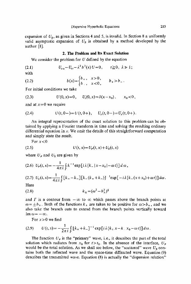
The function Ue is the "primary" wave, i.e., it describes the part of the total solution which radiates from Xo for t > to. In the absence of the interface, Up would be the total solution. As we shall see below, the "scattered" wave U s contains both the reflected wave and the space-time diffracted wave. Equation (9) describes the transmitted wave. Equation (8) is actually the "dispersion relation"

216 N. BLEISTEIN :

[8, 9, 12] for this equation with k+ corresponding to the range x > 0 and k_ corresponding to the range x < 0.

The function Ue has the following alternative representation

(2.10) Ue(t,x)={~Jo(2b-Vt2--(X--Xo)2), X--Xo<t X - X o > t ,

which can be derived from (2.6). In this form, however, the qualitative features of the asymptotic form of U e as described in the introduction are obscured. Although the asymptotic expansion of (2.10) is well known, we prefer instead to rederive the result from (2.6) as a prelude to our analysis of (2.7) and (2.9) and as an aid to our subsequent interpretation of the asymptotic solution. We shall use the method of steepest descent [5] to find the asymptotic solution, although the leading terms could as easily be obtained by the method of stationary phase [5]. These leading terms, however, would only account for the phenomenon of ordinary radiation from the source, as well as reflection from and transmission through the interface. The diffracted field will arise as a lower order term in the asymptotic expansion of Us.

It should he noted that all of the above integrals are zero for I X-Xol> t. Therefore, in all further considerations,

(2.11) [X-Xol<t ,

that is, we consider only the domain of influence of (0, Xo).

3. Asymptotic Expansion of Ur We shall apply the method of steepest descent to U e as given by (2.6). To do

this, we define

(3.1) tp(co) = i ( k_ Ix-xol-~ot}. The condition that ~o have a saddle point (tp' (w) = 0) is just the requirement that

(3.2) Ix - X o I = (k_/o~) t .

For each (t,x) in the domain (2.11) with x < 0 there are two saddle points ___co o, ego>b_. The paths of steepest descent through these saddle points are shown in Figure 3.1. Dashed lines are used to indicate the part of the descent contours lying on the lower Rieman sheet of k_. The contour F can be replaced by the integral along the paths of descent as indicated.

To leading order then, the asymptotic expansion of Up is given parametrically, with parameter ~Oo, by the equations

(3.3) Ue,,~(2n2b 2 mo 1 t)-l /ZRe[exp{i2(]//~o-~_ [X-Xol-coot)+in/4}] ,

(3.4) [X-Xol=ge(COo)t, g e ( O g o ) = ~ / ~ / O g o , Ogo>b_, x < 0 .

Here we use ]// to denote the positive square root, rather than the multivalued function k. Alternatively, we can use (3.4) to eliminate co o and can write

(3.5) Ue(t, x) ,~ (2n 2 b _)- 1/2 [t2 _ (x - Xo) 2] - 1/4 cos(2 b_ Vt 2 - ( x -Xo) 2 - n/a).

We defer an interpretation of this result to Section 7.


r IIJ

' I I I I I

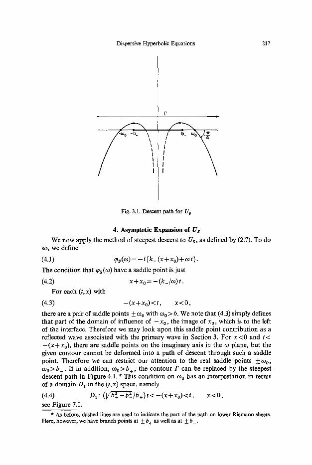
Fig. 3.1. Descent path for Up

4. Asymptotic Expansion of U s

We now apply the method of steepest descent to Us, as defined by (2.7). To do so, we define

(4.1) ~Ps (co) = - i {k_ (x + Xo) + r t}.

The condition that ~Ps (co) have a saddle point is just

(4.2) X + Xo--- -(k_/co) t.

For each (t, x) with

(4.3) -(X+Xo)<t, x < 0 ,

there are a pair of saddle points _+ co o with coo > b. We note that (4.3) simply defines that part of the domain of influence of - x o, the image of Xo, which is to the left of the interface. Therefore we may look upon this saddle point contribution as a reflected wave associated with the primary wave in Section 3. For x < 0 and t < - ( x + Xo), there are saddle points on the imaginary axis in the co plane, but the given contour cannot be deformed into a path of descent through such a saddle point. Therefore we can restrict our attention to the real saddle points -+coo, coo>b_. If in addition, coo>b+, the contour F can be replaced by the steepest descent path in Figure 4.1.* This condition on coo has an interpretation in terms of a domain D x in the (t,x) space, namely

(4.4) Dx: ( ] / ~ / b + ) t < - ( X + X o ) < t , x < 0 ,

see Figure 7.1.

* As before, dashed lines are used to indicate the part of the path on lower Riemann sheets. Here, however, we have branch points at _+ b+ as well as at -I- b .

218 N. BLEISTEIN :

I % + \ \ / / / /

i I

F

/ \ / \ I I I

Fig. 4.1. Descent path for Us, o~0>b +

l 1

I"

/ % ~ . / " b_ oJ o b,"~

i

Fig. 4.2. Descent path for Us, ~oo<b +

For b_ < O~o < b+, the contour F cannot be deformed onto a path of steepest descent without also introducing integrals enclosing the branch points _+_b+, see Figure 4.2. Consequently, we have another range of values D2 in the (t,x)-space,

(4.5) D2: -(X+Xo)<(~/~/b+)t, x < 0 ,

for which the asymptotic expansion of Us contains the saddle point contributions (the reflected wave) and another type of contribution arising from these integrals enclosing the branch points _b+. It is this latter contribution which we call the space-time diffracted wave. Before discussing the asymptotic form of the diffracted


wave, we shall find the leading term of the asymptotic expansion of the reflected wave, which we shall call UR. Parametrically, with parameter COo, we have

(4.6)

(4.7)

UR"~ Re {R (coo) (2 ~z 2 b 2 09o ~ t)- 2/2

�9 exp [ - i 2 { ] / ~ ( x + Xo) + OJo t} + i z c/a]},

X+xo=gs(090) t , gR(coo)=--Va~o--b2_/coo, coo>b_, x < 0 .

Here the "reflection coefficient" R (~Oo) is given by

(4.8) R(coo)= I V coo - b _ + ]/ coo-~- +

[ ]/~o-~2~_ + i 1 / ~ '

b+ <co o

b _ < c o o < b + .

(4.9)

where

Alternatively, we could eliminate the parameter oJ o and write

UR(t, x),-~ (2 rc 2 b_) - 1/2 [t 2 _ (x +Xo) 2] - 1/4

�9 Re {R (t, x) exp [ - i 2 b_ ]/t z - (x + Xo) z + i re/4] }

b_ Ix + Xo I - ] / b 2 (X + Xo)2- ( b2 - b 2) t2 (t, x) in D 1

b_ Ix + Xo I + 1/bZ+ (x + Xo) 2 - (bZ+ - bZ_) t 2 '

b _ I x + x 0 [ - i V(b 2 - b 2) t 2 - b 2 (x + Xo) 2 (t, x) in 0 2 .

(4.10) R(t , x ) =

b_ I X + Xo l + i V (b~+ -- b2 ) t2-- b2 (x + Xo) 2 '

5. The Diffracted Field

We now turn our attention to those contributions to U s arising from the integrals on the contours F 1, F 2 in Figure 4.2. Here (t ,x) is in the domain D 2 defined by (4.5). This contribution will be called the diffracted field Up. One can combine the two integrals in question into one along the contour F 1, and then can write

(5.1) Uo=2 Re W o

with

(5.2) Wo=[Tri( b2 - b 2 ) ] -x S k+ e x p [ - i 2 { k _ ( x + x o ) + O ~ t } ] do~. F1

Here, but for the small circle around the branch point b+ (the integral on this circle approaches 0 with the radius), the contour F 1 lies along a path of steepest descent away from b+. Therefore, we approximate the exponent, defined as q~s(co) in (4.1), by

(5.3) ~Os (co) ~ q~(b +) + tp' (b +) (co- b+)

and approximate k+ by

(5.4) k+ = (co z - b2) '/z ~ ]/2--b+ (09 - b +)1/2.

220 N. BLEISTEIN:

The change of variables c o - b + = a e 3n~12 now reduces the integral to one easily recognizable as a multiple of F(3/2)=l/n/2. Consequently, we find

Up'-' 2 ]//2-b--~+/n (b 2+ _ b2 ) - , [2 {(b + / V b + ~ - _ ) (x + Xo) + t)] -a/2

(5.5) �9 R e { e x p [ - i A { V b + ~ - _(X+Xo)+b + t}+3rri/4]}

for (t, x) in D2. We note that this asymptotic expansion is invalid near the boundary of D2, defined by equality in (4.5). Equivalently, this expansion is invalid when the stationary points _+ coo are "near" the branch points _+b+. In Section 8, an asymptotic expansion of U, + UR will be obtained having the feature that it remains uniformly valid up to the boundary of D2.

6. Asymptotic Solution for x > 0

The asymptotic solution for x > 0 is obtained by applying the method of steepest descent to (2.9). We define

(6.1) ~0r (co) = i [k+ x - k_ Xo- co t] .

This function has a saddle point whenever

k+ k+ (6.2) X=Xo k_ + co t.

Whenever x - X o < t and x > 0, (6.2) has a pair of solutions + coo with coo > b+. Here, the method of steepest descent yields a contribution which we shall call Ur, the transmitted wave. Parametrically, with parameter co o ,

[ b2+ b 2 ~ Xo b2+t ~-1/2 UT~ 2(2X 2)- 1/2 ].k ~ 0 - ~ - - + - - ~ ] ~ + coo (COo z - bZ-J

(6.3) . [ V ~ + V ~ o T ~ + ]_ 1

�9 cos [2 { l / ~ x - 1 / ~ x o -coo t} + Ir/4],

(6.4) x=gT(coo)t+ xoVcoo-~- +/]/coo-~- _ , gr(coo)=V~o--2---~- +/coo, coo>b+.

Here, as x ~ 0 , coo ~ b + and formally UT ~ 0 . However, b+ is a branch point of the exponent and not a saddle point, so that we cannot simply let x approach 0 in UT. Let us instead consider (2.9) for x = 0, and define the exponent to be

(6.5) 90 (co) = - i (k_ Xo + co t).

This exponent has saddle points whenever

(6.6) co o)2 b 2 t2 k_ x ~ = t --'2-~o"

Here t 2 > Xo 2 ' and therefore co is real. On the boundary of D 1 (see (4.4) with x = 0 , and Figure 7.1) we find that

(6.7) t 2_xo 2 < 2 2 b_/b+, c o 2 > b 2 + .


In this case one can readily calculate the saddle point contributions and find that asymptotically

(6.8) Ur(t, 0 + ) = Ue(t, 0 - ) + UR(t, 0 - ) .

From (2.6), (2.7) and (2.9) one can show the exact result

(6.9) Ur(t, 0)= Up(t, 0 - ) + Us(t, 0 - ) .

However, UR is the asymptotic expansion of U s in D1 and hence the equality in (6.8) holds to all orders in 2.

On the boundary of D E (see (4.5) with x = 0 , and Figure 7.1) one can verify that

(6.10) b 2 < 092 < b 2 "

Also (6.8) is still satisfied. Let us consider x "small", but positive and in the continuation of D 2 to X > 0. In this case we have the saddle points _+ 090, which lead to the contribution U r. In addition there are two complex saddle points which we shall call 09 • (x). As x ~ 0, these saddle points approach real numbers _+ o9 1, with 09~ given by (6.6) subject to (6.10).

By setting 09 = 09• (x) in (6.2), differentiating (6.2) with respect to x, and evalu- ating at x = 0, one can show that

(6.1 1) d 09dx • (x) x = 0 - -2 i 09~ 2 k2 (091) b_ Vb + -092 t

We conclude that Im 09• ( x )<0 for 0 < x ,~ 1. One can also show that

(6.12) Re q~(09+ (x))< 0= Re ~P (-+ 090),

i.e., that 09• (x) are in the "valleys" of -+090. Consequently, we can find paths of descent through _ 090 which include paths of descent through to • (x), see Figure 6.1.

/ ! I I

F ID

I I

F i g . 6.1

16 Arch. Rational Mech. Anal., Vol. 31

222 N. BLEISTEIN :

Let us define U e ( t , x ) , the evanescent wave, as the contribution to U r ( t , x ) arising from the complex saddle points 09~-(x). We have such a contribution for all (t, x) in the continuation of D2 for which the descent path in Figure 6.1 can be used. Equivalently, (6.12) must be satisfied. The boundary of this domain is determined by the equality in (6.12) subject to the condition (6.2). The problem of determination of this boundary is not readily solved. However, we note from (6.12) that UE decays exponentially for x > 0 . Therefore, for x small, let us determine the exponent and amplitude of UE as power series in x and retain only the leading term of the phase (imaginary part of the exponent), the decay factor (real part of the exponent), and the amplitude.* For example, with q~ given by (6.1), we write

(6.13) q ~ ( 0 9 ~ ( x ) , x ) = ~ o ( + w l , 0 ) + x ~ Ox ~- x=o +O(x2)"

After some algebra, the right side of (6.13) can be reduced to

V -b_)t - b + x o (6.14) c p ( 0 9 + ( x ) , x ) = + _ i b _ ] / t ~ - o - X (b2 2 2 2 2 t2 x 2 q - O ( x 2 ) �9

We can also calculate the leading term of 8 2 ~o/009 2 at 09 = 09 • (x), as well as the amplitude in (2.9). We then find that for x small

U n ~ 2 R e f (2 rc 2 b - a)- l/Z xo ( -,'o/'~2~- 1/4 I-fh2 i_k~, + - b 2_ ) t 2 - b +2 x20 _ i b_ xo] - i

(6.15) .exp i 2 b _ V ~ - x ~ - 2 x - t 2 _ x ~ +3re

7. Interpretation: The Space-Time Diffracted Wave

For x < 0 we have obtained an asymptotic solution

(7.1) U = U p + U R + U o

with each term of the form Re [A exp [i~k]]. We shall now give an interpretation of this result in the style of geometrical optics.

For each wave, i~O is just the exponent ~0 of the integral representation, multi- plied by + 2 and evaluated at a saddle point or branch point.

Let us consider the phase of Up in (3.5), i.e.

(7.2) ~Op = - 2 b_ ] / t 2 - (x - Xo) 2 .

Also we define the frequency

(7.3) 2 v = -- 0 ~p/8 t = 2 b_ t / l / t 2 - (x - Xo) 2

and observe that 2 v is constant (2 v = 2COo) on the lines defined by (3.5). We shall call these lines "primary rays"; observe that they fill out the characteristic cone [ X - X o l < t as 09o varies in the range b _ < 0 9 o < ~ , see Figure 7.1. Now let us define the wave number

(7.4) 2 x = 0 ~b e/O x = ~. b_ (x - Xo)/~/ t ~ - (x - Xo) 2

* For larger values of x we could simply set Ug=0.

Dispersive Hyperbol ic Equa t ions 223

and observe that on the primary rays

(7.5) x2(0%) =c02 - b 2 ,

that is

(7.6) x(e~o) = k_ (~o).

Now we see that ge(O)o) in (3.4) is simply the "group speed" [7, 8, 9],

(7.7)

\ \ \ \ \

TRANSMITTED .AYs

=t A

X o 0

Fig. 7.1. Diffracted rays shown as dashed lines

i

We now look upon (4.7) as defining a family of "reflected rays" with group speed gR(Wo) and (6.7) as defining "transmitted rays" with group speed gT(a~o). The spreading of these rays in Figure 7.1 characterizes the fact that the group speed is frequency dependent in a dispersive medium. The rays become steeper (the group speed decreases) with decreasing co o . In particular, for co o =b + , which is the lower limit of values of co o in x > 0, the transmitted ray is verticle, i.e., it is " t rapped" at

the interface. Let us now consider U o as defined by (5.5). Here we have a wave at the fixed

frequency 2b+ being "shed" from the interface for all times past the time ta of arrival at the interface of the primary wave with frequency 2b+. We may look upon this wave as being shed by the trapped part of U r . To complete our ray picture, we simply observe that we can associate the group speed gg(b+) with this wave and simply draw the corresponding rays emanating from the interface for all times t > t a . Here t a is obtained by setting both sides equal in (4.5) and also setting x = 0; thus

(7.8) t a = - Xo b + / l /b +~- _ .

16"

224 N. BLEISTEIN:

An observer at some fixed x < 0 will see two waves of varying frequency passing him, the primary and the reflected wave. In addition he will see a smaller wave Uo at fixed frequency, 2b+, with amplitude decreasing in time.

We have called the term Uo a space-time diffracted eave. This is motivated by the similarity with the problem of an accoustic or electro-magnetic wave emanating from a line source and incident on a plane boundary (see, for example, [3, 7]). There the critical frequency is replaced by a critical angle of incidence. Transmitted rays in that case are referred to as refracted rays, and our trapped ray is simply the ray refracted at an angle n/2 in that problem. The analogue of Uo is alternatively called a lateral wave or diffracted wave in that case. In [9], LEwis shows how asymptotic solutions of dispersive hyperbolic equations can be obtained by using the methods of geometrical optics which, up until recently, had been applied only to elliptic equations [6, 7, 8, 10, 11 ]. In using this method one assumes a solution as a sum of terms of the form

(7.9) u ,-~ A (t, x; 2) exp [i 2 @ (t, x)] .

Here A is assumed to be an inverse power series in 2. When (7.9) is substituted into the differential equation and the coefficients of 2 2 and ;t are set equal to zero, one obtains a "dispersion relation" and a "transport equation" which are the analogs of the "eikonal equation" and "transport equation" for elliptic equations.

For (2.1) the dispersion equation is

(7.10) k2=(.o2-b(x) 2, k-- i//z, r -i//t .

This is a first order non-linear partial differential equation for @ which can be solved by the method of characteristics. The characteristics for (7.10) are of course just the rays described above. One then determines A and ~, as solutions of ordinary differential equations along the rays.

One difficulty with this method is that the "initial" values of A and ~, on the rays are not always indicated by the given problem. In particular, this happens when one seeks the asymptotic solution for a diffracted wave in the form (7.9). To find these initial values one can resort to a "canonical problem", i.e., a problem which is simpler than the given problem but retains the same essential features in the neighborhood of the initial manifold of the rays (see, for example, [6, 7, 9, 10, 11]). The problem considered here could be viewed as a canonical problem for the more difficult situation where b(x) is some varying function of x, with b+ ( b ) the right (left) limits of b(x) at a discontinuity. Our results for U, and UE at x=O then serve to determine the initial values on the rays for the diffracted and evanescent waves in this more difficult problem. In addition one must assume a decay exponent for UE in the general problem; it too can be determined from our results here.

8. Uniform Asymptotic Expansion of Us In Section 5, we noted that the asymptotic expansion of Up was not valid near

the boundary of the region D2 defined by (4.5). Equivalently this expansion is not valid when the stationary point co o is near the branch point b+. This same difficulty arises when one computes lower order terms in the asymptotic expansion of UR.


Here we shall obtain an asymptotic expansion (of Us = UR + Uo) which remains uniformly valid as we approach the boundary of D2, or equivalently as o9o approaches b+. The method to be applied was developed by the author [1] and was actually motivated by consideration of this problem.

We consider the expression U s as defined by (2.7), and first deform F onto a path F' for which the decay of the exponent guarantees the convergence of the integral�9 A contour such as the one shown in Figure 4.1 will suffice, whether or not O9o > b + , i.e., whether (t,x) is in D1 or Dz. We then rewrite Us in the form

(8.1) Us=UI +U2, where

(8.2) U1 = -[4ni(b2+-bZ-)] -1S k-l[2o92-b2+ -b2-] exp [2 q~s] dog, F '

(8.3) U2=[ani(bZ+-b2_)] - I ~ k+ exp [2 ~0s] de). F '

Here q~s is given by (4�9 The integrand in (8.2) has no branch point at b+, and hence no difficulty arises as (t, x) passes from the domain D 1 to D2, or, equivalently, as o) o passes through b+. Therefore we can immediately obtain the asymptotic expansion of Ut by the method of steepest descent�9 Parametrically, with parameter ~o o ,

U 1 ,-~ [2re 2 b z t o9o 1] -1/2 [2 ogoZ- b2+ -b2_] [bE -bZ_] -~

(8.4) �9 cos [2 { 1 , / ~ (x + Xo) + o9o t} - zr/4] ;

(8.5) X+Xo= -gv(ogo) t, gv (mo)=V~o~-_ /ogo , COo > b.

Equivalently, if we eliminate the parameter 090,

U 1 (t, x) ~ [2 ~ 2 b_ (t 2 - (x + Xo)2) 3] -1/2 [(b2+ _ b2_) t2 + (x + Xo) 2 (b2+ + b 2_)] (8.6)

�9 cos [2 b_ V tz - (x + Xo) 2 - rc/4].

We now consider the integral U 2 . For o9o bounded away from b+, U z is 0(2-1/2), while for o) o = b +, U2 = O (2- 3/4). We shall obtain a uniform asymptotic expansion of Uz which exhibits this change in algebraic order as O9o- b+.

One can readily show that

(8.7) U2 = Re {[2~ i(bZ+ - bg_)]-I I} ,

(8.8) I = I k+ exp [2 q~s] dog. F1

Following [1], we set

(8.9) ~o s (o9) - q~s (b +) = - [z2/2 + a z] .

Here z = 0 when o9 = b + and z = - a when o9 = o9 o . Consequently

(8.10) aZ=2 [Cps(ogo)-q~s(b + )] . From (4.1) and (4.7)

(8.11) Cps(ogo)= -i[Vwo-y---ff'f- _ (x + xo)+ogot]= - i b_ V t 2 - ( X + Xo) 2,

(8.12) q~s(b+)= - i [ ] /b+~- _(X+Xo)+b+ t].

226 N. BLEISTEIN:

We apply the method in [1], Section 6, to choose the proper square root in (8.10) to define a. The result is

(8.13) a= +_exp[i~/4]V21q~s(too)-q~s(b+)l, __+(b+-to0)>0.

C ii

ot:l

- o

Fig. 8.1. Image path in v plane

In Figure 8.1 we show the image contour C in the z plane and the position of the saddle point - a , for to o < b. For this choice the change of variables remains one-to-one and analytic near C even when too passes through b+ or a passes through zero.

Now we have

(8.14) I = e x p [2 tp(b+)] S z l / 2 G ( z ) e x p [ - 2 ( z z / 2 + a z ) ] d z . C

Here

(8.15) dto T 1/2 de '

and this function is regular in a domain containing the contour C. Again using [1], we set

(8.16) G(z)=yo + h z + O ( z ( z + a ) ) .

Here

(8.17) ~0= G(0), h=a-~[G(O)-G(-a)], with

(8.18) G(O)=exp[ -3r r i / 8 ]V2b+[ la lVb+~- - / I b + ( x + x o ) + V ~ [ ] 3/2

and

(8.19) G ( - a) = exp [ - 3 rc i/8] b- ~ [(to2 _ b2)/a (x + Xo) l 1/2 (b 2 - b2) 3/'.

Both ~o and )'1 have finite limits as too ~ b+. Also, according to [1], the leading term of the uniform asymptotic expansion of I arises from the sum of integrals obtained by replacing G in (8.14) by ~o and ~ t. These integrals are expressible in terms of the Weber function of imaginary arguments [12]. In particular, for this


problem, we need the result

(8.20) S zr exp[-(z2/2+sz)]dr=exp[s2/4+rni/2]V2-~Dr(is) c

with Dr(z) defined in [12]�9 Consequently

Re _f exp [2(~o s2__~_~+ ~ ~ ( ~ 1 7 6 + ~o s (b +))/2 - ~ i/4] } U1 (8.21)

�9 [Yo 01/2 (i ] / /2a) + i Yl ~- 1/2 D3/2 (i V-2a)]. A t the boundary of D2, U2=0(2 -3/4) while U1=0(2-1/2), and in fact U I = U,. Away f rom the boundary we can use the asymptotic expansion of the Weber function to verify that the sum of the asymptotic expansions of U1 and U 2 yields the asymptotic expansion of Us.

Acknowledgement. This research was supported in part by the National Science Foundation and in part by the Office of Naval Research under contract No. Nonr 285(48).

References 1. BLEISTEIN, N., Uniform asymptotic expansion of integrals with stationary point near algebraic

singularity. Comm. Pure Appl. Math. 19, 353-- 370 (1966). 2. BLEISTEIN, N., & R. M. LEWIS, Space-time diffraction for dispersive hyperbolic equations.

SIAM J. Appl. Math. 14, 1454-- 1470 (1966). 3. BREKHOVSKIKH, L. M., Waves in Layered Media. New York: Academic Press 1960, pp. 270--

292. 4. COURANT, R., & D. HILBERT, Methods of Mathematical Physics, II. New York: Interscience

Publishers 1962. 5. ERDELYI, A., Asymptotic Expansions. New York: Dover Publications 1956. 6. KELLER, J.B., The geometrical theory of diffraction. J. Opt. Soc. Amer. 52, 116-- 130 0962). 7�9 KELLER, J.B., R.M. LEWIS, & ]3. SECKLER, Asymptotic solutions of some diffraction prob-

lems. Comm. Pure Appl. Math. 9, 207--265 (1956). 8. LANDAU, L.D., & E.M. LIFSHITZ, Electrodynamics of Continuous Media. New York: Per-

gamon Press 1960. 9. LEWIS, R.M., Asymptotic Methods for the Solution of Dispersive Hyperbolic Equations.

In: Asymptotic Solutions of Differential Equations and Their Applications, edited by C. WILCOX. New York: Wiley 1964, pp. 53-- 107.

10. SECKLER, B.D., & J. B. KELLER, Geometrical theory of diffraction in inhomogeneous media. J. Acoust. Soc. Amer. 31, 192--205 (1959).

11. SECKLER, B.D., • J.B. KELLER, Asymptotic theory of diffraction in inhomogeneous media. J. Acoust. Soc. Amer. 31, 206--216 (1959).

12. WHITHAM, G.B., Group velocity and energy propagation for three dimensional waves. Comm. Pure Appl. Math. 14, 675--691 (1961).

Department of Mathematics Massachusetts Institute

of Technology

(Received June 25, 1968)

diffraction in the asymptotic solution of a dispersive hyperbolic equation

Documents