differentiating discretized metrics and applications filelogo the continuous framework applications...
TRANSCRIPT

logo
The continuous frameworkApplications
DiscretizationResults
Differentiating discretized metrics and applications
Filippo Santambrogio
Laboratoire de Mathematiques d’Orsay, Universite Paris-Sudhttp://www.math.u-psud.fr/∼santambr/
PICOF – April 3rd, 2012, Ecole Polytechnique
Filippo Santambrogio Differentiating discretized metrics and applications
logo
The continuous frameworkApplications
DiscretizationResults
1 The continuous framework
Distances and Eikonal EquationGeodesics appear when differentiating
2 Applications
Slow down the opposantTravel-time tomographyTraffic congestion equilibria
3 Discretization
FMMDerivative computation
4 Results
Slow down the opposantTravel-time tomographyTraffic congestion equilibria
Filippo Santambrogio Differentiating discretized metrics and applications
logo
The continuous frameworkApplications
DiscretizationResults
The continuous frameworkRiemannian distances and geodesics
Filippo Santambrogio Differentiating discretized metrics and applications

logo
The continuous frameworkApplications
DiscretizationResults
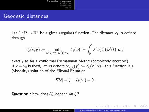
Geodesic distances
Let ξ : Ω→ R+ be a given (regular) function. The distance dξ is definedthrough
dξ(x , y) := infω(0)=x, ω(1)=y
Lξ(ω) :=
∫ 1
0
ξ(ω(t))|ω′(t) |dt,
exactly as for a conformal Riemannian Metric (completely isotropic).If x = x0 is fixed, let us denote Ux0,ξ(y) := dξ(x0, y) : this function is a(viscosity) solution of the Eikonal Equation
|∇U| = ξ, U(x0) = 0.
Question : how does Uξ depend on ξ ?
Filippo Santambrogio Differentiating discretized metrics and applications

logo
The continuous frameworkApplications
DiscretizationResults
Geodesic distances
Let ξ : Ω→ R+ be a given (regular) function. The distance dξ is definedthrough
dξ(x , y) := infω(0)=x, ω(1)=y
Lξ(ω) :=
∫ 1
0
ξ(ω(t))|ω′(t) |dt,
exactly as for a conformal Riemannian Metric (completely isotropic).If x = x0 is fixed, let us denote Ux0,ξ(y) := dξ(x0, y) : this function is a(viscosity) solution of the Eikonal Equation
|∇U| = ξ, U(x0) = 0.
Question : how does Uξ depend on ξ ?
Filippo Santambrogio Differentiating discretized metrics and applications
logo
The continuous frameworkApplications
DiscretizationResults
Concavity, derivatives and subgradients
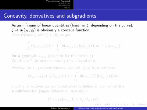
As an infimum of linear quantities (linear in ξ, depending on the curve),ξ 7→ dξ(x0, y0) is obviously a concave function.If we replace ξ with ξ + εh, we get
d
dεUx0,ξ+εh(y) =
∫ 1
0
h(ωx0,y (t))|ω′x0,y (t)| dt = Lh(ωx0,y ),
for a geodesic ωx0,y (geodesic for the metric ξ).Which one ? the one minimizing this integral of h.
Anyway, for all geodesic curve ω connecting x0 to y , we have
Ux0,ξ+εh(y) ≤ Ux0,ξ(y) + ε
∫ 1
0
h(ωx0,y (t))|ω′x0,y (t)| dt,
and the derivatives we computed allow to define an element of thesubdifferential (super-differential, actually) :(
h 7→ Lh(ωx0,y ))∈ ∂−ξ Ux0,ξ(y).
Filippo Santambrogio Differentiating discretized metrics and applications
logo
The continuous frameworkApplications
DiscretizationResults
Concavity, derivatives and subgradients
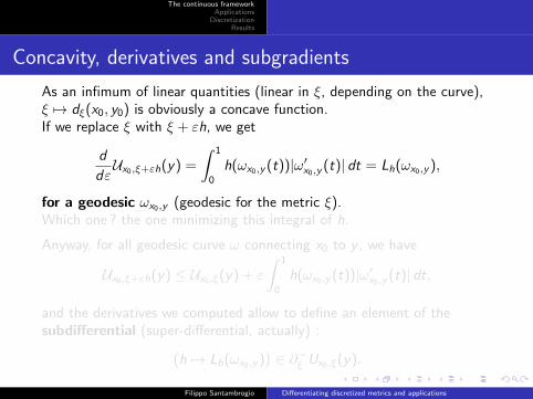
As an infimum of linear quantities (linear in ξ, depending on the curve),ξ 7→ dξ(x0, y0) is obviously a concave function.If we replace ξ with ξ + εh, we get
d
dεUx0,ξ+εh(y) =
∫ 1
0
h(ωx0,y (t))|ω′x0,y (t)| dt = Lh(ωx0,y ),
for a geodesic ωx0,y (geodesic for the metric ξ).Which one ? the one minimizing this integral of h.
Anyway, for all geodesic curve ω connecting x0 to y , we have
Ux0,ξ+εh(y) ≤ Ux0,ξ(y) + ε
∫ 1
0
h(ωx0,y (t))|ω′x0,y (t)| dt,
and the derivatives we computed allow to define an element of thesubdifferential (super-differential, actually) :(
h 7→ Lh(ωx0,y ))∈ ∂−ξ Ux0,ξ(y).
Filippo Santambrogio Differentiating discretized metrics and applications
logo
The continuous frameworkApplications
DiscretizationResults
Concavity, derivatives and subgradients
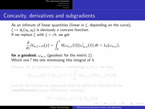
As an infimum of linear quantities (linear in ξ, depending on the curve),ξ 7→ dξ(x0, y0) is obviously a concave function.If we replace ξ with ξ + εh, we get
d
dεUx0,ξ+εh(y) =
∫ 1
0
h(ωx0,y (t))|ω′x0,y (t)| dt = Lh(ωx0,y ),
for a geodesic ωx0,y (geodesic for the metric ξ).Which one ? the one minimizing this integral of h.
Anyway, for all geodesic curve ω connecting x0 to y , we have
Ux0,ξ+εh(y) ≤ Ux0,ξ(y) + ε
∫ 1
0
h(ωx0,y (t))|ω′x0,y (t)| dt,
and the derivatives we computed allow to define an element of thesubdifferential (super-differential, actually) :(
h 7→ Lh(ωx0,y ))∈ ∂−ξ Ux0,ξ(y).
Filippo Santambrogio Differentiating discretized metrics and applications

logo
The continuous frameworkApplications
DiscretizationResults
Concavity, derivatives and subgradients
As an infimum of linear quantities (linear in ξ, depending on the curve),ξ 7→ dξ(x0, y0) is obviously a concave function.If we replace ξ with ξ + εh, we get
d
dεUx0,ξ+εh(y) =
∫ 1
0
h(ωx0,y (t))|ω′x0,y (t)| dt = Lh(ωx0,y ),
for a geodesic ωx0,y (geodesic for the metric ξ).Which one ? the one minimizing this integral of h.
Anyway, for all geodesic curve ω connecting x0 to y , we have
Ux0,ξ+εh(y) ≤ Ux0,ξ(y) + ε
∫ 1
0
h(ωx0,y (t))|ω′x0,y (t)| dt,
and the derivatives we computed allow to define an element of thesubdifferential (super-differential, actually) :(
h 7→ Lh(ωx0,y ))∈ ∂−ξ Ux0,ξ(y).
Filippo Santambrogio Differentiating discretized metrics and applications

logo
The continuous frameworkApplications
DiscretizationResults
Applications
Optimization involving dξ
Filippo Santambrogio Differentiating discretized metrics and applications
logo
The continuous frameworkApplications
DiscretizationResults
Why would we need to differentiate w.r.t. ξ ?
Obviously, to solve optimization problems involving the distances dξ.
To write optimality conditions. . . and/or apply a gradient descentalgorithm (and sub-gradient descent is also good).
But we can also use to define some evolution of metrics, for instance, orto impose topological constraints on unknown shapes.
Filippo Santambrogio Differentiating discretized metrics and applications

logo
The continuous frameworkApplications
DiscretizationResults
The so-called “military applications”
Here’s a problem posed by Buttazzo et al. : find the optimal metric ξ soas to slow down an opposant located at y0 who wants to attack ourstronghold at x0 (under suitable constraints) :
max
dξ(x0, y0),
∫ξ ≤ M, a ≤ ξ ≤ b
.
If a = 0 and Ω is large enough the solution is obtained by setting ξ = b
on two equal balls around x0 and y0 and ξ = 0 elsewhere.What about a > 0 ?
G. Buttazzo, A. Davini, I. Fragala and F. Macia, Optimal Riemannian
distances preventing mass tranfer, J. Reine Angew. Math., 2004.
Filippo Santambrogio Differentiating discretized metrics and applications

logo
The continuous frameworkApplications
DiscretizationResults
Travel-time tomography
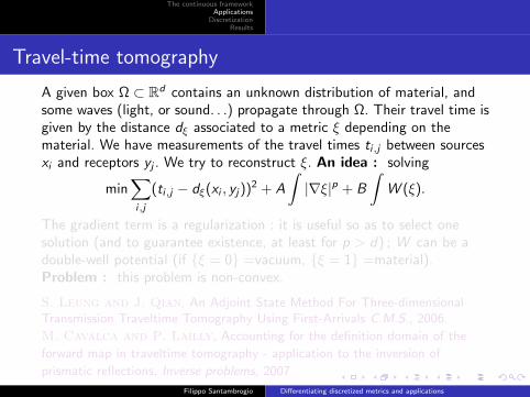
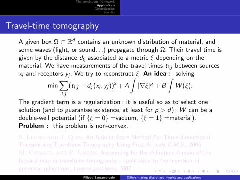
A given box Ω ⊂ Rd contains an unknown distribution of material, andsome waves (light, or sound. . .) propagate through Ω. Their travel time isgiven by the distance dξ associated to a metric ξ depending on thematerial. We have measurements of the travel times ti,j between sourcesxi and receptors yj . We try to reconstruct ξ. An idea : solving
min∑i,j
(ti,j − dξ(xi , yj))2 + A
∫|∇ξ|p + B
∫W (ξ).
The gradient term is a regularization : it is useful so as to select onesolution (and to guarantee existence, at least for p > d) ; W can be adouble-well potential (if ξ = 0 =vacuum, ξ = 1 =material).Problem : this problem is non-convex.
S. Leung and J. Qian, An Adjoint State Method For Three-dimensionalTransmission Traveltime Tomography Using First-Arrivals C.M.S., 2006.
M. Cavalca and P. Lailly, Accounting for the definition domain of the
forward map in traveltime tomography - application to the inversion of
prismatic reflections, Inverse problems, 2007
Filippo Santambrogio Differentiating discretized metrics and applications

logo
The continuous frameworkApplications
DiscretizationResults
Travel-time tomography
A given box Ω ⊂ Rd contains an unknown distribution of material, andsome waves (light, or sound. . .) propagate through Ω. Their travel time isgiven by the distance dξ associated to a metric ξ depending on thematerial. We have measurements of the travel times ti,j between sourcesxi and receptors yj . We try to reconstruct ξ. An idea : solving
min∑i,j
(ti,j − dξ(xi , yj))2 + A
∫|∇ξ|p + B
∫W (ξ).
The gradient term is a regularization : it is useful so as to select onesolution (and to guarantee existence, at least for p > d) ; W can be adouble-well potential (if ξ = 0 =vacuum, ξ = 1 =material).Problem : this problem is non-convex.
S. Leung and J. Qian, An Adjoint State Method For Three-dimensionalTransmission Traveltime Tomography Using First-Arrivals C.M.S., 2006.
M. Cavalca and P. Lailly, Accounting for the definition domain of the
forward map in traveltime tomography - application to the inversion of
prismatic reflections, Inverse problems, 2007
Filippo Santambrogio Differentiating discretized metrics and applications

logo
The continuous frameworkApplications
DiscretizationResults
Traffic congestion - definitions
We consider the distribution of a set of commuters over possible paths asa probability Q ∈ P(C ), where C = ω : [0, 1]→ Ω, ω ∈ C 0,1 is the setof curves in Ω. To every Q we can associate a traffic intensityiQ ∈M+(Ω) (a positive measure on Ω) through
< iQ , φ >=
∫C
Lφ(ω)Q(dω).
If iQ = iQ(x)dx is actually absolutely continuous (diffuse), then we definea metric ξQ = g(x , iQ(x)), where g : Ω× R+ → R+ is given such thati 7→ g(x , i) is increasing and stands for the sensitivity of x to trafficintensity.
We prescribe the number of agents commuting from x to y for every pair(x , y) ∈ Ω× Ω, i.e. we fix (π0,1)#Q where π0,1 : C → Ω× Ω is givenbyπ0,1(ω) = (ω(0), ω(1)). The equilibrium problem reads as
“Find Q, with given marginal (π0,1)#Q = γ such that iQ is diffuseand Q is concentrated on the set of geodesics for the metric ξQ .”
G. Carlier, C. Jimenez , F. Santambrogio, Optimal transportation with
traffic congestion and Wardrop equilibria, SICON, 2008.Filippo Santambrogio Differentiating discretized metrics and applications

logo
The continuous frameworkApplications
DiscretizationResults
Traffic congestion - theorems
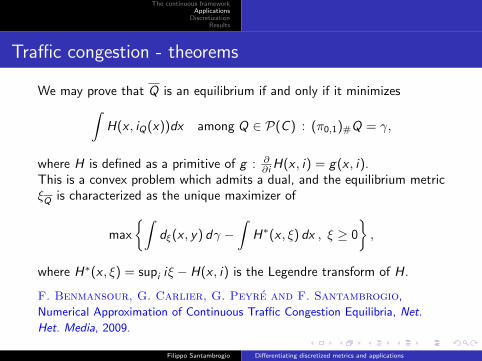
We may prove that Q is an equilibrium if and only if it minimizes∫H(x , iQ(x))dx among Q ∈ P(C ) : (π0,1)#Q = γ,
where H is defined as a primitive of g : ∂∂i H(x , i) = g(x , i).
This is a convex problem which admits a dual, and the equilibrium metricξQ is characterized as the unique maximizer of
max
∫dξ(x , y) dγ −
∫H∗(x , ξ) dx , ξ ≥ 0
,
where H∗(x , ξ) = supi iξ − H(x , i) is the Legendre transform of H.
F. Benmansour, G. Carlier, G. Peyre and F. Santambrogio,
Numerical Approximation of Continuous Traffic Congestion Equilibria, Net.
Het. Media, 2009.
Filippo Santambrogio Differentiating discretized metrics and applications
logo
The continuous frameworkApplications
DiscretizationResults
Traffic congestion - theorems
We may prove that Q is an equilibrium if and only if it minimizes∫H(x , iQ(x))dx among Q ∈ P(C ) : (π0,1)#Q = γ,
where H is defined as a primitive of g : ∂∂i H(x , i) = g(x , i).
This is a convex problem which admits a dual, and the equilibrium metricξQ is characterized as the unique maximizer of
max
∫dξ(x , y) dγ −
∫H∗(x , ξ) dx , ξ ≥ 0
,
where H∗(x , ξ) = supi iξ − H(x , i) is the Legendre transform of H.
F. Benmansour, G. Carlier, G. Peyre and F. Santambrogio,
Numerical Approximation of Continuous Traffic Congestion Equilibria, Net.
Het. Media, 2009.
Filippo Santambrogio Differentiating discretized metrics and applications

logo
The continuous frameworkApplications
DiscretizationResults
DiscretizationUpwind schemes for distances and gradients
Filippo Santambrogio Differentiating discretized metrics and applications

logo
The continuous frameworkApplications
DiscretizationResults
Distance computations on a grid
On a regular square grid with step h > 0, we look for a discretization ofthe solution f the Eikonal equation |∇U| = ξ. It is well known that if thevalues Ui,j solve the Discrete Eikonal system
(DE ) (DxU)2i,j+(DyU)2
i,j = (ξi,j)2 ,
where we define
(DxU)i,j := max(Ui,j − Ui−1,j), (Ui,j − Ui+1,j), 0/h,
(DyU)i,j := max(Ui,j − Ui,j−1), (Ui,j − Ui,j+1), 0/h,
then they give a good approximation of the true viscosity solution (withconvergence as h→ 0).
E. Rouy and A. Tourin. A viscosity solution approach to shape from
shading. SIAM Journal on Numerical Analysis, 1992.
Filippo Santambrogio Differentiating discretized metrics and applications

logo
The continuous frameworkApplications
DiscretizationResults
Fast Marching Method
The previous system is usually solved through the so-called FastMarching Method. All the points are classified as known, trial, or far andtheir status is updated during the algorithm, as well as their value of U .Algorithm
Set U(x0) = 0 and the status of x0 to trial ; for all the other pointsset Ui,j = +∞ and their status to far.
Repeat until there is at least a point which is not known :1 Find the trial point y with minimal value of U ,2 Change the status of y from trial to known,3 Change the status of the neighbors of y from far to trial (if they are
not already trial),4 Compute the values of Ui,j for (i , j) neighbor of y according to (DE).
The values of U solve the system.
If the grid has N points, the computational cost for that is O(N ln N).J. A. Sethian Level Set Methods and Fast Marching Methods. Cambridge
University Press, 1999.
Filippo Santambrogio Differentiating discretized metrics and applications
logo
The continuous frameworkApplications
DiscretizationResults
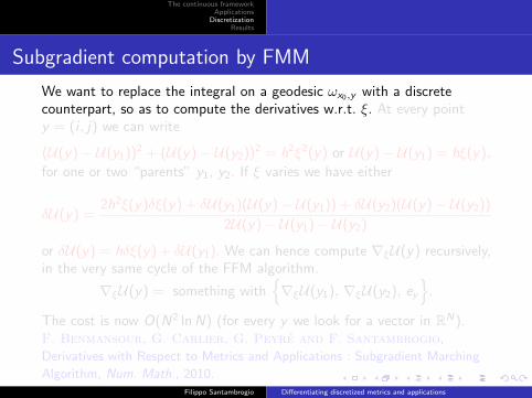
Subgradient computation by FMM
We want to replace the integral on a geodesic ωx0,y with a discretecounterpart, so as to compute the derivatives w.r.t. ξ. At every pointy = (i , j) we can write
(U(y)− U(y1))2 + (U(y)− U(y2))2 = h2ξ2(y) or U(y)− U(y1) = hξ(y),
for one or two “parents” y1, y2. If ξ varies we have either
δU(y) =2h2ξ(y)δξ(y) + δU(y1)(U(y)− U(y1)) + δU(y2)(U(y)− U(y2))
2U(y)− U(y1)− U(y2)
or δU(y) = hδξ(y) + δU(y1). We can hence compute ∇ξU(y) recursively,in the very same cycle of the FFM algorithm.
∇ξU(y) = something with∇ξU(y1), ∇ξU(y2), ey
.
The cost is now O(N2 ln N) (for every y we look for a vector in RN).F. Benmansour, G. Carlier, G. Peyre and F. Santambrogio,
Derivatives with Respect to Metrics and Applications : Subgradient Marching
Algorithm, Num. Math., 2010.Filippo Santambrogio Differentiating discretized metrics and applications

logo
The continuous frameworkApplications
DiscretizationResults
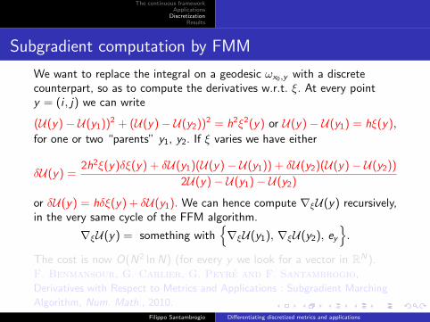
Subgradient computation by FMM
We want to replace the integral on a geodesic ωx0,y with a discretecounterpart, so as to compute the derivatives w.r.t. ξ. At every pointy = (i , j) we can write
(U(y)− U(y1))2 + (U(y)− U(y2))2 = h2ξ2(y) or U(y)− U(y1) = hξ(y),
for one or two “parents” y1, y2. If ξ varies we have either
δU(y) =2h2ξ(y)δξ(y) + δU(y1)(U(y)− U(y1)) + δU(y2)(U(y)− U(y2))
2U(y)− U(y1)− U(y2)
or δU(y) = hδξ(y) + δU(y1). We can hence compute ∇ξU(y) recursively,in the very same cycle of the FFM algorithm.
∇ξU(y) = something with∇ξU(y1), ∇ξU(y2), ey
.
The cost is now O(N2 ln N) (for every y we look for a vector in RN).F. Benmansour, G. Carlier, G. Peyre and F. Santambrogio,
Derivatives with Respect to Metrics and Applications : Subgradient Marching
Algorithm, Num. Math., 2010.Filippo Santambrogio Differentiating discretized metrics and applications

logo
The continuous frameworkApplications
DiscretizationResults
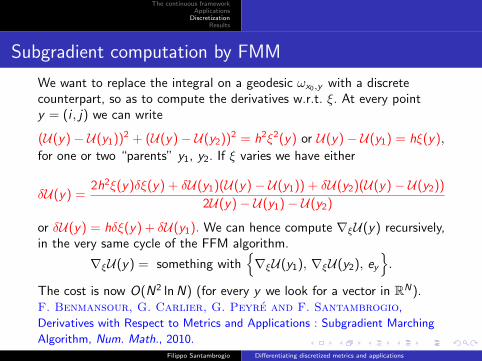
Subgradient computation by FMM
We want to replace the integral on a geodesic ωx0,y with a discretecounterpart, so as to compute the derivatives w.r.t. ξ. At every pointy = (i , j) we can write
(U(y)− U(y1))2 + (U(y)− U(y2))2 = h2ξ2(y) or U(y)− U(y1) = hξ(y),
for one or two “parents” y1, y2. If ξ varies we have either
δU(y) =2h2ξ(y)δξ(y) + δU(y1)(U(y)− U(y1)) + δU(y2)(U(y)− U(y2))
2U(y)− U(y1)− U(y2)
or δU(y) = hδξ(y) + δU(y1). We can hence compute ∇ξU(y) recursively,in the very same cycle of the FFM algorithm.
∇ξU(y) = something with∇ξU(y1), ∇ξU(y2), ey
.
The cost is now O(N2 ln N) (for every y we look for a vector in RN).F. Benmansour, G. Carlier, G. Peyre and F. Santambrogio,
Derivatives with Respect to Metrics and Applications : Subgradient Marching
Algorithm, Num. Math., 2010.Filippo Santambrogio Differentiating discretized metrics and applications

logo
The continuous frameworkApplications
DiscretizationResults
Subgradient computation by FMM
We want to replace the integral on a geodesic ωx0,y with a discretecounterpart, so as to compute the derivatives w.r.t. ξ. At every pointy = (i , j) we can write
(U(y)− U(y1))2 + (U(y)− U(y2))2 = h2ξ2(y) or U(y)− U(y1) = hξ(y),
for one or two “parents” y1, y2. If ξ varies we have either
δU(y) =2h2ξ(y)δξ(y) + δU(y1)(U(y)− U(y1)) + δU(y2)(U(y)− U(y2))
2U(y)− U(y1)− U(y2)
or δU(y) = hδξ(y) + δU(y1). We can hence compute ∇ξU(y) recursively,in the very same cycle of the FFM algorithm.
∇ξU(y) = something with∇ξU(y1), ∇ξU(y2), ey
.
The cost is now O(N2 ln N) (for every y we look for a vector in RN).F. Benmansour, G. Carlier, G. Peyre and F. Santambrogio,
Derivatives with Respect to Metrics and Applications : Subgradient Marching
Algorithm, Num. Math., 2010.Filippo Santambrogio Differentiating discretized metrics and applications
logo
The continuous frameworkApplications
DiscretizationResults
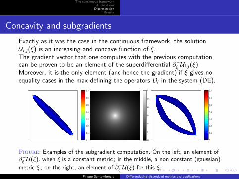
Concavity and subgradients
Exactly as it was the case in the continuous framework, the solutionUi,j(ξ) is an increasing and concave function of ξ.The gradient vector that one computes with the previous computationcan be proven to be an element of the superdifferential ∂−ξ Ui,j(ξ).Moreover, it is the only element (and hence the gradient) if ξ gives noequality cases in the max defining the operators Di in the system (DE).
0
0.1
0.2
0.3
0.4
0.5
0.6
0.7
0.8
1
1.2
1.4
1.6
1.8
2
0
0.1
0.2
0.3
0.4
0.5
0.6
0.7
Figure: Examples of the subgradient computation. On the left, an element of∂−ξ U(ξ). when ξ is a constant metric ; in the middle, a non constant (gaussian)
metric ξ ; on the right, an element of ∂−ξ U(ξ) for this ξ.
Filippo Santambrogio Differentiating discretized metrics and applications

logo
The continuous frameworkApplications
DiscretizationResults
ResultsObstacle optimization, tomography and traffic
Filippo Santambrogio Differentiating discretized metrics and applications
logo
The continuous frameworkApplications
DiscretizationResults
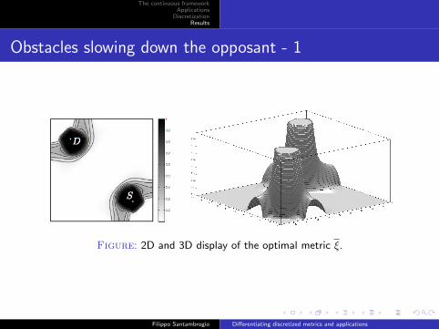
Obstacles slowing down the opposant - 1
Figure: 2D and 3D display of the optimal metric ξ.
Filippo Santambrogio Differentiating discretized metrics and applications
logo
The continuous frameworkApplications
DiscretizationResults
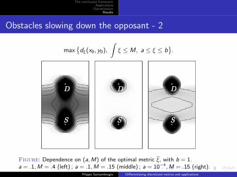
Obstacles slowing down the opposant - 2
max
dξ(x0, y0),
∫ξ ≤ M, a ≤ ξ ≤ b
.
Figure: Dependence on (a,M) of the optimal metric ξ, with b = 1.a = .1,M = .4 (left) ; a = .1,M = .15 (middle) ; a = 10−4,M = .15 (right).
Filippo Santambrogio Differentiating discretized metrics and applications
logo
The continuous frameworkApplications
DiscretizationResults
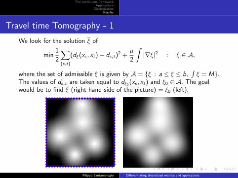
Travel time Tomography - 1
We look for the solution ξ of
min1
2
∑(s,t)
(dξ(xs , xt)− ds,t)2 +
µ
2
∫|∇ξ|2 : ξ ∈ A,
where the set of admissible ξ is given by A = ξ : a ≤ ξ ≤ b,∫ξ = M.
The values of ds,t are taken equal to dξ0 (xs , xt) and ξ0 ∈ A. The goalwould be to find ξ (right hand side of the picture) = ξ0 (left).
Filippo Santambrogio Differentiating discretized metrics and applications

logo
The continuous frameworkApplications
DiscretizationResults
Travel time Tomography - 2
An example with points inside the domain. Notice that∫|∇ξ|2 is
discretized in the easiest way :∫|∇ξ|2 =
∑i,j
(ξi+1,j − ξi,j)2 + (ξi,j+1 − ξi,j)2.
ξ0 ξ
Figure: Examples of travel time tomography recovery.
Filippo Santambrogio Differentiating discretized metrics and applications

logo
The continuous frameworkApplications
DiscretizationResults
Traffic equilibria - 1
−2
−1.5
−1
−0.5
0
0.5
Figure: Two sources and two targets, with a river and a bridge on asymmetric configuration and an asymmetric traffic weights.
Filippo Santambrogio Differentiating discretized metrics and applications

logo
The continuous frameworkApplications
DiscretizationResults
Traffic equilibria- 2
Figure: Running of the subgradient algorithm
Filippo Santambrogio Differentiating discretized metrics and applications
logo
The continuous frameworkApplications
DiscretizationResults
The End . . .. . . thanks for your attention
Filippo Santambrogio Differentiating discretized metrics and applications