Differential EquationsMTH 242

Lecture # 13

Dr. Manshoor Ahmed

Summary (Recall)

• Differential Operator, which is a linear operator.

• Differential equation in linear operator form.

• Auxiliary equation in terms of differential operator form.

• Annihilator operator.

• Annihilator operators of different functions.

• Solution non-homogeneous equation with annihilator operator.

Method of variation of parameters

dxxfePdxeyPdx

p ..

Pdxey1

,0 yxPdx

dy

xycy 11

1 1 py u x y x

dy P x y f xdx

xfdx

duyyxP

dx

dyu

1

111

1

11 0

dyP x y

dx

So that we obtain

This is a variable separable equation.

Thus,

 

Integration gives

  .

As .

Therefore,

or .

11

duy f x

dx

1

1

f xdu dx

y x

11

( )Pdxf x

u x dx e f x dxy

dxxfPdxePdxey p ..

1

1

f xu dx

y x

1 1 py u x y x

Method for Second Order Equation:We consider the second order linear non-homogeneous DE

Divide by , to get equation in the standard form

,

where

are continuous on some interval I.

Consider the associated homogeneous DE,

.

xgyxayxayxa 012

)(2 xa

xfyxQyxPy

01

2 2 2

( )( ) ( )( ) , ( ) , ( )

( ) ( ) ( )

a xa x g xP x Q x f x

a x a x a x

0 yxQyxPy

Complementary function:

Complementary function is

So that

Particular Integral

For finding a particular solution , we replace the parameters

and in the complementary function with the unknown variables

and . So that the assumed particular integral is

xycxycyc 2211

1 1 1

2 2 2

0

0

y P x y Q x y

y P x y Q x y

py 1c

2c

xu1 2u x

1 1 2 2py u x y x u x y x

Since we seek to determine two unknown functions and ,

we need two equations involving these unknowns. One of

these two equations results from substituting the assumed in the

given differential equation. We impose the other equation to

simplify the first derivative and thereby the 2nd derivative of

To avoid 2nd derivatives of and , we impose the condition

Then,

So that

Therefore,

1 u

py

2 u

py

2211221122221111 yuyuyuyuyuyuuyyuy p

1 u 2 u

02211 yuyu

2211 yuyuy p

22221111 yuyuyuyuy p

2211̀2211

22221111

yQuyQuyPuyPu

yuyuyuyuyQyPy ppp

Substituting in the given non-homogeneous differential equation yields

 

or

Now making use of the relations

we get,

Hence and must be functions that satisfy the equations

By using the Cramer’s rule, the solution of this set of equations is given by

)( 2211̀221122221111 xfyQuyQuyPuyPuyuyuyuyu

)(][] [ 21122221111 xfyuyuQyyPyuyQyPyu

1 1 1

2 2 2

0

0

y P x y Q x y

y P x y Q x y

xfyuyu 22111 u 2 u

1 1 2 2

1 1 2 2

0

u y u y

u y u y f x

1 21 2,

W Wu u

W W

where and denote the following determinants

The determinant can be identified as the Wronskian of the

solutions . Since the solutions are linearly

independent on I. Therefore

Now integrating the expressions for we obtain the value of and , hence the particular solution of the non-homogeneous

linear DE.

Summary of the Method

To solve the second order non-homogeneous linear DE

using the variation of parameters, we need to perform the following steps:

1 2,W W andW

W

2 11 21 2

2 11 2

0 0, ,

y yy yW W W

f x y y f xy y

21 and yy 21 and yy

. ,0, 21 IxxyxyW

1 2u andu

1 u 2 u

,012 xgyayaya

Step 1 We find the complementary function by solving the associated

homogeneous differential equation

Step 2 If the complementary function of the equation is given by

then are two linearly independent solutions of the

homogeneous differential equation. Computing Wronskian.

Step 3 By dividing with , we transform the given non-homogeneous

equation into the standard form

and we identify the function f(x).

0012 yayaya

2211 ycyccy 21 and yy

21

21

yy

yyW

2a

xfyxQyxPy

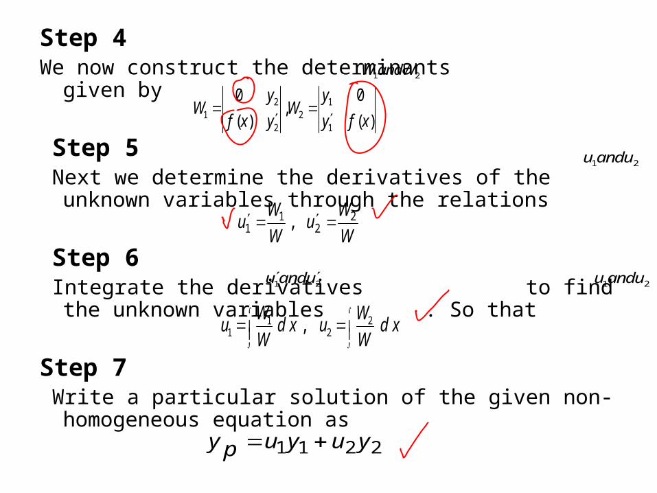
Step 4 We now construct the determinants given by

Step 5 Next we determine the derivatives of the unknown variables

through the relations

Step 6 Integrate the derivatives to find the unknown variables

. So that

Step 7 Write a particular solution of the given non-homogeneous

equation as

1 2W andW

2 11 2

2 1

0 0,

( ) ( )

y yW W

f x y y f x

1 2u andu

W

Wu

W

Wu 2

21

1 ,

1 2u andu 1 2u andu

1 21 2 ,

W Wu d x u d x

W W

2211 yuyupy

Step 8 The general solution of the differential equation is then given by

 

Constants of IntegrationWe don’t need to introduce the constants of integration, when

computing the indefinite integrals in step 6 to find the unknown functions of . For, if we do introduce these constants, then

So that the general solution of the given non-homogeneous differential equation is

or

22112211 yuyuycycpycyy

1 1 1 2 1 2( ) ( )py u a y u b y

1 1 1 2 1 2 1 1 2 2y c a y c b y u y u y

2121112211 ybuyauycycyyy pc

1 2u andu

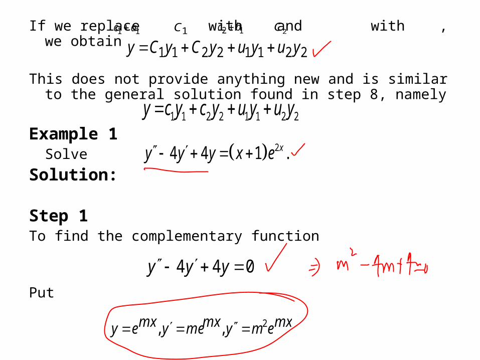
If we replace with and with , we obtain

This does not provide anything new and is similar to the general solution found in step 8, namely

Example 1Solve

Solution:  

Step 1 To find the complementary function

Put

11 ac 1C 2 1c b 2C

22112211 yuyuyCyCy

1 1 2 2 1 1 2 2y c y c y u y u y

24 4 1 .xy y y x e

044 yyy

mxemymxmeymxey 2,,

Then the auxiliary equation is

Repeated real roots of the auxiliary equation

Step 2 By the inspection of the complementary function , we make the

identification

Therefore

2

2

4 4 0

2 0, 2, 2

m m

m m

2 21 2 x x

cy c e c xe

cy

xx xeyey 22

21 and

xeexee

xeexeeyyW x

xxx

xxxx

,0

22, , 4

222

2222

21

Step 3 The given differential equation is

Since this equation is already in the standard form

Therefore, we identify the function as

Step 4 We now construct the determinants

xexyyy 2144

xfyxQyxPy

xexxf 2 1

24

1 2 2 2

24

2 2 2

01

1 2

01

2 1

xx

x x x

xx

x x

xeW x xe

x e xe e

eW x e

e x e

Step 5 We determine the derivatives of the functions in this step

Step 6 Integrating the last two expressions, we obtain

Remember! We don’t have to add the constants of integration.

Step 7 Therefore, a particular solution of then given differential

equation is

1 2u andu

1

1

1

4

42

2

24

41

1

xe

ex

W

Wu

xxe

xex

W

Wu

x

x

x

x

.2

)1(

23

)(

2

2

232

1

xx

dxxu

xxdxxxu

xxexxxe

xxpy 2

2

22

2

2

3

3

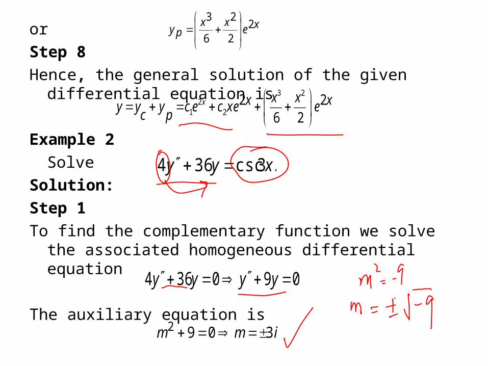
or

Step 8

Hence, the general solution of the given differential equation is

Example 2

Solve

Solution:

Step 1

To find the complementary function we solve the associated homogeneous differential equation

The auxiliary equation is

xexx

py 22

2

6

3

3 22

1 22 2

6 2x x xx xy y y c e c xe e

c p

.3csc364 xyy

090364 yyyy

imm 3092

Roots of the auxiliary equation are complex. Therefore, the complementary function is

Step 2 From the complementary function, we identify

as two linearly independent solutions of the associated

homogeneous equation. Therefore

Step 3 By dividing with , we put the given equation in the following

standard form

So that we identify the function as

xcxccy 3sin3cos 21

3sin ,3cos 21 xyxy

33cos33sin3

3sin3cos3sin,3cos

xx

xxxxW

.3csc4

19 xyy

xxf 3csc4

1

Step 4 We now construct the determinants

Step 5 Therefore, the derivatives are given by

Step 6 Integrating the last two equations w.r.t , we obtain

Here, no constants of integration are used.

xuxu 3sinln36

1 and

12

121

1

2

0 sin 31 1

csc3 sin 314 4csc3 3cos3

4

cos3 01 cos3

14 sin 33sin 3 csc3

4

xW x x

x x

xx

Wxx x

x

x

W

Wu

W

Wu

3sin

3cos

12

1 ,

12

1 22

11

1 2W andW

1 2u andu

Step 7 The particular solution of the non-homogeneous equation is

Step 8 Hence, the general solution of the given differential equation is

Example 3Solve

Solution: Step 1 For the complementary function consider the associated

homogeneous equation

To solve this equation we put

1 1cos3 sin 3 ln sin 3

12 36y x x x xp

xxxxxcxcpycyy 3sinln3sin36

13cos

12

13sin3cos 21

.1

xyy

0 yy

mxmxmx emyemyey 2, ,

Then the auxiliary equation is:

The roots of the auxiliary equation are real and distinct. Therefore, the complementary function is

Step 2 From the complementary function we find

The functions are two linearly independent solutions of the homogeneous equation. The Wronskian of these solutions is

Step 3 The given equation is already in the standard form

 

1012 mm

xecxeccy 21

xeyxey 21 ,

2

,

xx

xxxx

ee

eeeeW

y p x y Q x y f x

21 and yy

Here  

Step 4 We now form the determinants

Step 5 Therefore, the derivatives of the unknown functions and are

given by

Step 6 We integrate these two equations to find the unknown functions

xxf

1)(

)/1( /1

0 W

)/1( /1

0 W

2

1

xexe

e

xeex

e

xx

x

xx

x

11

22

1/

2 2

1/

2 2

x x

x x

e xW eu

W x

e xW eu

W x

1 2

1 1,

2 2

x xe eu dx u dx

x x

1 2u andu

The integrals defining cannot be expressed in terms of the elementary functions and it is customary to write such integral as:

Step 7 A particular solution of the non-homogeneous equations is

Step 8 Hence, the general solution of the given differential equation is

1 2u andu

1 2

1 1,

2 2

x xt t

xx

e eu dt u dt

t t

x

x

x

x

tx

tx

p dtt

eedt

t

eey

2

1

2

1

x

x

tx

x

x

txxx dt

t

eedt

t

eeececpycyy

2

1

2

121

For practice solve the problems from Exercise 4.6

of your text book

Summary

• Motivation for the method of variation of parameters.

• Method for first order DEs.

• Method for second order DEs.

• Summary of the method.

• No need to add the constants.

• Some examples.