differential equations - college of computingdifferential equation: x˙ (t)=kx(t) numerical...
TRANSCRIPT

Differential Equations


• Overview of differential equation
• Initial value problem
• Explicit numeric methods
• Implicit numeric methods
• Modular implementation

Physics-based simulation
• It’s an algorithm that produces a sequence of states over time under the laws of physics
• What is a state?
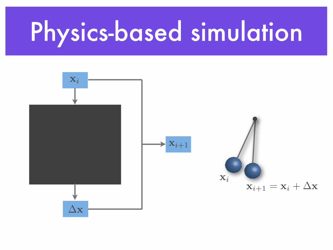
Physics-based simulationxi
!x
xi+1
xi+1 = xi + !x
xi

Physics-based simulationxi
!x
xi+1
xi
xi+1 = xi + !x
Newtonian lawsgravity
wind gust
elastic force.
.
.
integrator

Differential equations
• What is a differential equation?
• It describes the relation between an unknown function and its derivatives
• Ordinary differential equation (ODE)
• is the relation that contains functions of only one independent variable and its derivatives

Ordinary differential equations
An ODE is an equality equation involving a function and its derivatives
What does it mean to “solve” an ODE?
x(t) = f(x(t))
known function
time derivative of the unknown function
unknown function that evaluates the state given time
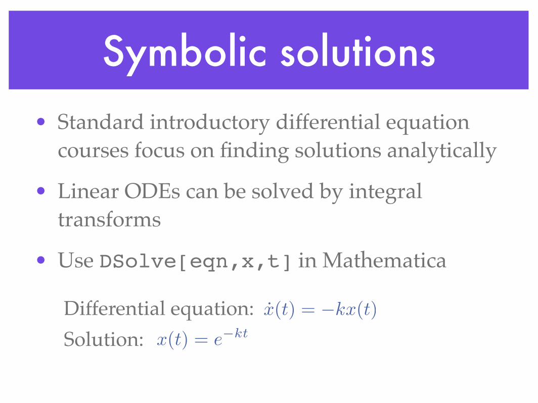
Symbolic solutions• Standard introductory differential equation
courses focus on finding solutions analytically
• Linear ODEs can be solved by integral transforms
• Use DSolve[eqn,x,t] in Mathematica
Solution: x(t) = e
�kt
Differential equation: x(t) = �kx(t)

Numerical solutions
• In this class, we will be concerned with numerical solutions
• Derivative function f is regarded as a black box
• Given a numerical value x and t, the black box will return the time derivative of x

Physics-based simulationxi
!x
xi+1
xi
xi+1 = xi + !x
Newtonian lawsgravity
wind gust
elastic force.
.
.
integrator

• Overview of differential equation
• Initial value problem
• Explicit numeric methods
• Implicit numeric methods
• Modular implementation

Initial value problemsIn a canonical initial value problem, the behavior of the system is described by an ODE and its initial condition:
x = f(x, t)
x(t0) = x0
To solve x(t) numerically, we start out from x0 and follow the changes defined by f thereafter

Vector field
The differential equation can be visualized as a vector field
x = f(x, t)
x2
x1


Vector field
How does the vector field look like if f depends directly on time?
The differential equation can be visualized as a vector field
x = f(x, t)
x2
x1

Integral curves
f(x, t)
!t0
f(x, t)dt

Physics-based simulationxi
!x
xi+1
xi
xi+1 = xi + !x
Newtonian lawsgravity
wind gust
elastic force.
.
.
integrator

• Overview of differential equation
• Initial value problem
• Explicit numeric methods
• Implicit numeric methods
• Modular implementation

Explicit Euler method
Discrete time step h determines the errors
Instead of following real integral curve, p follows a polygonal path
How do we get to the next state from the current state?
x(t0 + h) = x0 + hx(t0)x(t0 + h)
x(t0)p

Problems of Euler method
Inaccuracy
The circle turns into a spiral no matter how small the step size is

Problems of Euler method
Instability
How small the step size has to be?
Oscillation:
Divergence:
x = !kx
x(t) = e!ktSymbolic solution:

Accuracy of Euler method
• At each step, x(t) can be written in the form of Taylor series:
• What is the order of the error term in Euler method?
• The cost per step is determined by the number of evaluations per step
x(t0 + h) = x(t0) + hx(t0) +h2
2!x(t0) +
h3
3!x
(3)(t0) + . . .hn
n!
!nx
!tn
Taylor series is a representation of a function as an infinite sum of terms calculated using the
derivatives at a particular point

Stability of Euler method
• Assume the derivative function is linear
• Look at x parallel to the largest eigenvector of A
• Note that eigenvalue can be complex
d
dtx = Ax
d
dtx = !x
!

The test equation
• Test equation advances x by
• Solving gives
• Condition of stability
xn+1 = xn + h!xn
xn = (1 + h!)nx0
|1 + h!| ! 1

Stability region• Plot all the values of hλ on the complex plane
where Euler method is stable

Real eigenvalue• If eigenvalue is real and negative, what kind of
the motion does x correspond to?
• a damping motion smoothly coming to a halt
• The threshold of time step
• What about the imaginary axis?h !
2
|!|

Imaginary eigenvalue
• If eigenvalue is pure imaginary, Euler method is unconditionally unstable
• What motion does x look like if the eigenvalue is pure imaginary?
• an oscillatory or circular motion
• We need to look at other methods

The midpoint method
2. Evaluate f at the midpoint
3. Take a step using fmid
fmid = f(x(t0) +!x
2)
1. Compute an Euler step!x = hf(x(t0))
x(t0 + h) = x(t0) + hfmid
x(t + h) = x0 + hf(x0 +h
2f(x0))
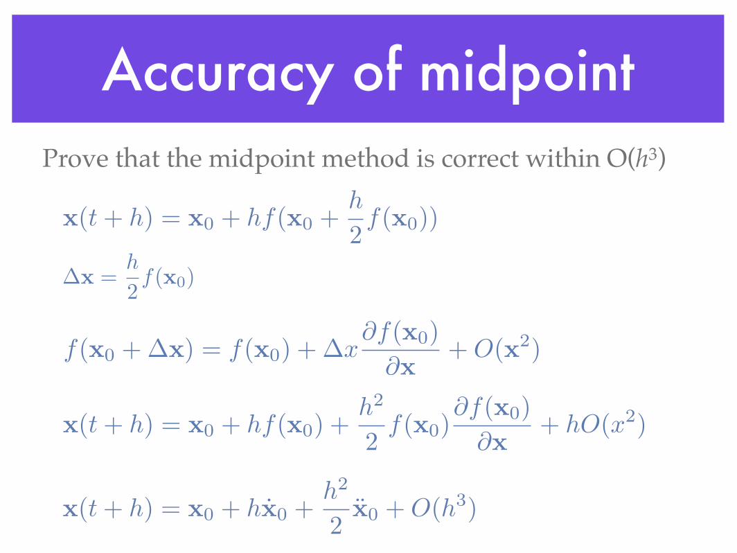
Accuracy of midpointProve that the midpoint method is correct within O(h3)
x(t + h) = x0 + hf(x0 +h
2f(x0))
x(t + h) = x0 + hx0 +h2
2x0 + O(h3)
x(t + h) = x0 + hf(x0) +h2
2f(x0)
!f(x0)
!x
+ hO(x2)
!x =h
2f(x0)
f(x0 + !x) = f(x0) + !x!f(x0)
!x
+ O(x2)

Stability regionxn+1 = xn + h!x
n+ 1
2
= xn + h!(xn +1
2h!xn)
xn+1 = xn(1 + h! +1
2(h!)2)
h! = x + iy
!
!
!
!
"
1
0
#
+
"
x
y
#
+1
2
"
x2 ! y
2
2xy
#!
!
!
!
" 1
!
!
!
!
"
1 + x +x2!y
2
2
y + xy
#!
!
!
!
! 1

Stability of midpoint• Midpoint method has larger stability region, but
still unstable on the imaginary axis

Runge-Kutta method
• Runge-Kutta is a numeric method of integrating ODEs by evaluating the derivatives at a few locations to cancel out lower-order error terms
• Also an explicit method: xn+1 is an explicit function of xn
Runge-Kutta method
• q-stage p-order Runge-Kutta evaluates the derivative function q times in each iteration and its approximation of the next state is correct within O(hp+1)
• What order of Runge-Kutta does midpoint method correspond to?

4-stage 4th order Runge-Kutta
f(x0, t0)
f(x0 +k1
2, t0 +
h
2)
f(x0 +k2
2, t0 +
h
2)
f(x0 + k3, t0 + h)
x0
x(t0 + h)
2.
1.
3.
4.
k1 = hf(x0, t0)k2 = hf(x0 + k1
2, t0 + h
2)
k3 = hf(x0 + k2
2, t0 + h
2)
k4 = hf(x0 + k3, t0 + h)x(t0 + h) = x0 + 1
6k1 + 1
3k2 + 1
3k3 + 1
6k4
t
x

High order Runge-Kutta• RK3 and up are include part of the imaginary axis

Stage vs. order
p 1 2 3 4 5 6 7 8 9 10qmin(p) 1 2 3 4 6 7 9 11 12-17 13-17
The minimum number of stages necessary for an explicit method to attain order p is still an open problem
Why is fourth order the most popular Runge Kutta method?

Adaptive step size
• Ideally, we want to choose h as large as possible, but not so large as to give us big error or instability
• We can vary h as we march forward in time
• Step doubling
• Embedding estimate
• Variable step, variable order

Step doubling
e
xb = xtemp +h
2f(xtemp, t0 +
h
2)
xtemp = x0 +h
2f(x0, t0)
Estimate by taking a full Euler stepxa
Estimate by taking two half Euler stepsxb
e = |xa ! xb| is bound by O(h2)
Given error tolerance , what is the optimal step size?!
!
!
e
"1
2
h
xa = x0 + hf(x0, t0)

Embedding estimate
• Also called Runge-Kutta-Fehlberg
• Compare two estimates of
• Fifth order Runge-Kutta with 6 stages
• Forth order Runge-Kutta with 6 stages
x(t0 + h)

Variable step, variable order
• Change between methods of different order as well as step based on obtained error estimates
• These methods are currently the last work in numerical integration

Problems of explicit methods
• Do not work well with stiff ODEs
• Simulation blows up if the step size is too big
• Simulation progresses slowly if the step size is too small

Example: a bead on the wire
Y =d
dt
!
x(t)y(t)
"
=
!
!x(t)!ky(t)
"
Ynew =
!
(1 ! h)x(t)(1 ! kh)y(t)
"
Ynew = Y0 + hY(t0) =
!
x(t)y(t)
"
+ h
!
!x(t)!ky(t)
"
Explicit Euler’s method:
Y(t) = (x(t), y(t))y(t)
x(t)

Stiff equations
• Stiffness constant: k
• Step size is limited by the largest k
• Systems that has some big k’s mixed in are called “stiff system”

• Overview of differential equation
• Initial value problem
• Explicit numeric methods
• Implicit numeric methods
• Modular implementation

Implicit methods
Implicit Euler: Ynew = Y0 + hf(Ynew)
Explicit Euler: Ynew = Y0 + hf(Y0)
Solving for such that ! , at time , points directly back at !! !
fYnewt0 + h
Y0

Implicit methods
Ynew = Y0 + hf(Y0) + h!Yf !(Y0)
!Y =
!
1
hI ! f !(Y0)
""1
f(Y0)
Approximating f(Ynew) by linearizing f(Y)
f(Ynew) = f(Y0) + !Yf !(Y0) !Y = Ynew ! Y0, where
Our goal is to solve for Ynew such thatYnew = Y0 + hf(Ynew)
f(Y, t) = Y(t)
f(Y, t)� =⇥f
⇥Y

Example: A bead on the wire
Apply the implicit Euler method to the bead-on-wire example
!Y =
!
1
hI ! f !(Y0)
""1
f(Y0)
=
!
!1 0
0 !k
"
f !(Y(t)) =!f(Y(t))
!Y
f(Y(t)) =
!
!x(t)!ky(t)
"
!Y =
!
1+h
h0
0 1+kh
h
"
!1 !
!x0
!ky0
"
=
!
h
h+10
0h
1+kh
" !
!x0
!ky0
"
= !
!
h
h+1x0
h
1+khky0
"

Example: A bead on the wire
What is the largest step size the implicit Euler method can take?
limh!"
!Y = limh!"
!
!
h
h+1x0
h
1+khky0
"
= !
!
x0
1
kky0
"
= !
!
x0
y0
"
Ynew = Y0 + (!Y0) = 0

Stability of implicit Euler• Test equation shows stable when
• How does the stability region look like?
|1 ! h!| " 1

Problems of implicit Euler
• Implicit Euler could be stable even when physics is not!
• Implicit Euler damps out motion unrealistically

Implicit vs. explicit
correct solution: x(h) = e!hk
implicit Euler: x(h) =1
1 + hk
explicit Euler: x(h) = 1 ! hk
h
x(h) = !kx(h)x(0) = 1
x

Trapezoidal rule
• Take a half step of explicit Euler and a half step of implicit Euler
• Explicit Euler is under-stable, implicit Euler is over-stable, the combination is just right
xn+1 = xn + h(1
2f(xn) +
1
2f(xn+1))

Stability of Trapezoidal
• What is the test equation for Trapezoidal?
• Where is the stability region?
• negative half-plane
• Stability region is consistent with physics
• Good for pure rotation
h! ! 0

Terminology
• Explicit Euler is also called forward Euler
• Implicit Euler is also called backward Euler

• Overview of differential equation
• Initial value problem
• Explicit numeric methods
• Implicit numeric methods
• Modular implementation
Modular implementation• Write integrator in terms of
• Reusable code
• Simple system implementation
• Generic operations:
• Get dim(x)
• Get/Set x and t
• Derivative evaluation at current (x, t)

Solver interface
System (black box)
Solver (integrator)
GetDim
Deriv Eval
Get/Set State

Summary
• Explicit Euler is simple, but might not be stable; modified Euler may be a cheap alternative
• RK4 allows for larger time step, but requires much more computation
• Use implicit Euler for better stability, but beware of over-damp

What’s next?

• How do we use Euler method to simulate the motion of a mass point?
• What are the equations of motion when forces are applied to the mass point?
• Read: Differential equations, by Andy Witkin and David Baraff