differential equations and - diffjournal.spbu.rudiffjournal.spbu.ru/pdf/ansari.pdfdifferential...

DIFFERENTIAL EQUATIONS

AND

CONTROL PROCESSES № 1, 2013

Electronic Journal,

reg.Эл № ФС77-39410 at 15.04.2010 ISSN 1817-2172

http://www.math.spbu.ru/diffjournal

e-mail: [email protected]

Dynamical systems in medicine

Immune impairment and immunodeficiency thresholds in

HIV infection with general incidence rate

Hajar Ansari1 , Mahmoud Hesaaraki

2

1,2

Department of mathematics, Sharif University of Technology,

P.O.Box: 11155-9414,Tehran, Iran.

Abstract

In [1] and [2], the authors used a linear incidence rate into a mathematical model

to examine the immune impairment for a proliferation model of CTL responses in

the immune response to HIV. Under the assumption that the immune impairment

increases over the HIV infection, they classified four processes of the disease

progression dynamics, according to their virological properties. In particular they

showed that a typical disease progression presents a risky threshold and an

immunodeficiency threshold. Moreover the immune system might collapse when

the impairment rate of HIV exceeds a threshold value. On the other hand if the

immune impairment rate never exceeds the threshold value, the viral replication is

well controlled by CTL responses. In this paper we show that all of the above

results remain valid if we use a general functional response, instead of as

the incidence rate into the above mathematical model.

Keywords: HIV infection, Global stability, Functional response, Immune impairment,

immunodeficiency.

2010 Mathematics Subject Classification: 34D, 34E , 92B.

1 Introduction The origin of various disease progression in HIV(i.e. Human Immunodeficiency

Virus is a lentivirus(i.e. a member of retrovirus family, that causes acquired

1 E-mail address: [email protected]

2 E-mail address: [email protected]

http://www.math.spbu.ru/diffjournal

mailto:[email protected]

Differential Equations and Control Processes, № 1, 2013

Electronic Journal. http://www.math.spbu.ru/diffjournal 90

immunodeficiency syndrome,AIDS.) infection is largely unresolved but many

researchers have been trying to explain it. An important factor in understanding the

unusual incubation period distribution in the development of AIDS(i.e. Acquired

Immunodeficiency Syndrome) is the dynamics of the long-lasting struggle between HIV

and our immune system [3]. In early models of HIV infection [4] an explosion in the

virus load caused by increased HIV variants diversity explains the immune system

collapse in [5]. The CTL(i.e. Cytotoxic T Cells or killer T cell or Cytotoxic T-

lymphocyte are a sub-group of T cells which induce the death of cells that are infected

with viruses or are otherwise damaged or dysfunctional.) exhaustion induced by an

evolutionary increase of viral infectivity accounts for immune deficiency. Moreover, in

[6] the functional deteriorations of T and B cells caused by accumulations of deleterious

mutations are considered as a reason for development of AIDS.

In [1,2] the authors present discussion of an immune impairment effect caused by the

depletion and dysfunction of DC(i.e. Dendritic cells are immune cells forming part of

the mammalian immune system.) on HIV disease progression. Because the progressive

decrease of DC number and function during the course of HIV-1 is observed [7,8,9].

The authors in [1,2] simply assumed that the immune impairment effect increases over

HIV infection.

The authors in [1,2] by using the discussion of the immune impairment effect caused by

the depletion and dysfunction of DC on HIV disease program, extend the standard

virus-immune model including the effect of immune impairment cause by HIV infection

[4] to the following equations:

{

Here, and denote the concentration of the susceptible or uninfected

target cells, the exposed or infected cells that produce virus and the infective or HIV-1

virus particles at time , respectively. The positive constants and are

the proliferation rate of CD4+ T cells( i.e. helper T cells are immune response mediators

and play an important role in establishing and maximizing the capabilities of the

adaptive immune response. These cells have no cytotoxic or phagocytic activity and

cannot kill infected cells or clear pathogens, but in essence manage the immune

response, by directing other cells or perform these tasks.), the decay rate of infected

CD4+ T cells, the killing rate of infected CD4

+ T cells, the proliferation rate of CTLs,

the immune impairment rate of HIV and the decay rate of CTLs, per day, respectively.

Finally, is the incidence rate of the transmission of the infection or the rate of

infection and is a saturation response or functional response of uninfected cells

into the exposed cells.

Here we assume that the saturation response satisfies the following natural

hypotheses:

H1) .

H2 ) , for all .

H3 ) , for all .



Moreover we assume:

H4)

(

) , for all .

Notice that most of the famous functional responses such as: Lotka-Voltra, Michealis-

Menten, Holling type II, Holling type IV, Monod-Haldane, Ivlev and Rosenzweig

satisfy the above hypotheses. See the appendix.

The authors in [1] studied the mathematical analysis of the system (1.1) by assuming

that the rate of infection is bilinear i.e. . However, the actual incidence

rate is probably not linear over the entire range of . Thus, it is reasonable to assum that

the infected rate is given by one of the famous functional responses such as Michealis-

Menten, Holling type II and IV, Monod-Haldane, Ivlev and Rosenzweig. Since all of

these functional responses satisfy hypotheses H1-H4, we consider the system (1.1) with

the general functional response , for mathematical analysis investigation of HIV

infection.

In this paper, we will analyze the global stability of the viral free equilibrium and the

local and global stability of the infected equilibrium points for general incidence rate. In

fact, we will show that the results which are obtained in [2] remain valid for general

functional response, . In fact the model (1.1) has four possible equilibria:

uninfected equilibrium, shortage state equilibrium, immunodeficiency equilibrium and

controlled state equilibrium. In section 2, we consider the stability of the uninfected and

the shortage state equilibria. In section 3, we study the stability of the other equilibria.

In section 4, we will discuss the biological results.

2 Equilibrium Points and Stability In this section and the next one, we will find the equilibrium points of the system (1.1)

and then we will consider the stability property of them. In order to do this, we will find

the eigenvalues of the linearized system of this system at these points.

At an equilibrium point of the system (1.1) we must have

{

From the third equation we obtain or

.

In the following, we consider the case and the other case will be considered in

section 3.

By substituting into the second equation yields, . If , then

from the first equation we must have

. Thus

is one of the

equilibrium points which is called uninfected steady state of the system. If

, by using this in the first equation of (2.1) we get

. Hence at the second

equilibrium point, if exists we must have

By hypothesis, , we have . Since at an equilibrium point we must have

the acceptable root of (2.2) must be in the interval,

. Therefore the



second equilibrium point exists if and only if,

. Let

. This number is

called the basic reproductive ratio of the virus for the system. Thus we have the

following theorem.

Theorem 2.1 . For , if , then the uninfected steady state

is

the unique equilibrium point of the system (1.1). If , then in addition to the

uninfected steady state , there is another equilibrium point with

and .

Here we will analyze the local asymptotical stability of these equilibrium points. In

order to do this, we check the sign of the eigenvalues of Jacobi matrix of (1.1) at these

points. This matrix is given by

[

]

where .

At first we consider the local stability of the equilibrium point . Hence, we calculate

the eigenvalues of :

( )

[

]

Therefore, the eigenvalues of are the roots of the characteristic polynomial

( (

))

Thus, , (

) and are the eigenvalues of . Clearly,

and have negative real part. If, (

) , then the rest point is

locally asymptotically stable. This condition is the same as, . Therefore, we

have proved the following theorem.

Theorem 2.2. If , the equilibrium point is locally asymptotically stable and if

, this equilibrium point is unstable.

Now we will show that if , the equilibrium point is globally asymptotically

stable. First of all, consider the following domain in the space,

{ }

It follows from hypotheses and and the equations of the system (1.1), if an orbit

initiating on the boundary of , then this orbit gets into immediately as time

increases. This means that the flow generated by that system gets into on the

boundary of . Let , for

and consider the following set for :



{

}

where, (

)

, and

.

If we differentiate along the orbits of the system (1.1), we obtain:

(

)

[

]

Since on that part of the surface, which is some part of the boundary of

the set , we have and and

, therefore

. Thus, the flow gets into on

. Hence the flow gets into from its boundery. Therefore, if an orbit

starts outside of in , then that orbit must get into in a finite positive time. But,

. Hence, if an orbit start in , then it must approach to as time tends to

infinity. Hence we have proved the following theorem.

Theorem 2.3. If , then is the only rest point of the system (1.1). This rest

point is globally asymptotically stable.

Now we consider the local asymptotical stability of . Notice that from (2.3) we have

[

]

Therefore, the eigenvalues of are the roots of the characteristic polynomial

(

)

where and

. Thus,

is one of the

eigenvalues and the other two are the roots of . We call them

. We know that and . It follows from the hypotheses

, . Thus, and have negative real parts. So if

, then

the equilibrium is locally asymptotically stable. This is possible for as and

are independent of .

Therefore, we have proved the following theorem.



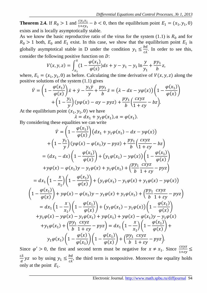
Theorem 2.4. If and

, then the equilibrium point

exists and is locally asymptotically stable.

As we know the basic reproductive ratio of the virus for the system (1.1) is and for

both, and exist. In this case, we show that the equilibrium point is

globally asymptotical stable in D under the condition

. In order to see this,

consider the following positive function on :

∫

where, as before. Calculating the time derivative of along the

positive solutions of the system (1.1) gives

(

)

( ) (

)

(

)

(

)

At the equilibrium point we have

By considering these equalities we can write

(

) ( )

(

)

(

)

(

) ( )(

)

(

)

(

) (

) ( )

(

) (

)

(

) (

) ( ) (

)

(

) (

) (

)

(

) (

) (

)

Since , the first and second term must be negative for . Since

so by using

, the third term is nonpositive. Moreover the equality holds

only at the point .



Since for and, and for

and , thus is a Lyapunov function of the system

(1.1) for on . Therefore, we have proved the following theorem.

Theorem 2.5. If the infected equilibrium point exists and

,

then this equilibrium point is globally asymptotically stable in . Remark 2.1. If Theorem 2.5 holds, and are all of the equilibrium points of the

system (1.1).

3 Other Equilibrium Points and Their Stability In this section, we will find the equilibrium points of the system (1.1) for and

. Then we will consider the stability of these points.

From

we obtain

and from the second equation of (2.1) we get

where . If , then the system (1.1) does not have any rest point in .

Hence we look for a rest point in the set .

By substituting from (3.1) into the first equation of (2.1) we obtain

(

)

Hence if (1.1) has another equilibrium point, it must satisfy in (3.1), (3.2) and (3.3). In

the following, we discuss in more detail about the existence of such solution. From (3.3)

we can write

(

)

The right hand side of (3.4) is a straight line and by hypothesis , the left hand side is a

concave upward curve with positive values.

If , then is negative in , but the left hand side of

(3.4) is positive. Therefore, in this case, the equation (3.4) does not have any solution.

This means that (3.3) cannot have any solution if .

If and is very small or , then as the concavity of

(

) does not change, the line intersects the

curve (

) in one point or two points. Hence (3.3) admits at most two

solutions in . Notice that the line is decreasing with respect to

and the curve

is increasing with respect to it. Thus if decreases these

two curves may intersect each others in two points.



If the line is tangent to the curve, then (3.4) and therefore, (3.3) has one solution. Hence

the system (1.1) admits another rest point. Let be this point, where

,

and satisfies in (3.4).

We show the corresponding to this rest point by . This number is called the

immunodeficiency threshold.

If , then the line cuts the curve in two different points and the equation (3.4) has

two different solutions. In this case, the system (1.1) has two other rest points. Let

be these points, with . Thus and . If

, then and are not in , but is in

for small values of . If

, then for and

for and small. That

is, there is an such that and is in

for . Thus

we have proved the following theorem.

Theorem3.1. If the line and the curve

intersect each other, then there is such that for and

for .

The number is called the risky threshold rate of immune impairment.

Now we consider the stability of . From (2.3) we have

[

] By

substituting

,

in (3.5) yield

[

]

where ( )

. Therefore, the characteristic polynomial of is

Where ,

( )

and

(

).

From the Routh-Hurwitz criterion, all eigenvalues have negative real parts if

By hypothesis , we have , thus and . Now we determine

the sign of and . Since satisfy in (3.4) and , at we have

( (

) )

By substituting

we get



(

)

By using (3.8) and (3.4) we obtain

(

) ( )

Hence, . Now we show that .

where (

).

Therefore, we establish the local asymptotical stability of .

For , at we have,

( (

) )

From the above inequality and

we obtain

(

)

Therefore, by using (3.16) and (3.4)

Since we conclude that the real part of one of three roots of the equation (3.14)

is positive. Hence, is always unstable. Therefore we have the following theorem.

Theorem 3.2. Suppose that the equilibrium exist. The equilibrium

point is always unstable and the equilibrium point is always locally

asymptotically stable.

4 Discussion The model which is given by the system (1.1) has four possible equilibria:

(

)

The basic reproductive number for one infected cell is definable as

, which

represents the average number of cells infected by a single infected cell in an otherwise

susceptible cell population.

In a healthy human only activated CD4+T cells attain an equilibrium level of

.

This homeostatic equilibrium is designated by in the above.

By Theorem 2.1, , the uninfected equilibrium or healthy state always exists and by

Theorem 2.2 for , it is the unique equilibrium and is globally asymptotically

stable. This means that the infected CD4+Tcells decreases to zero.



After infection of HIV, if , then infected CD4+T cells increase to high level and

uninfected CD4+T cells decrease to a low level. This situation is appeared by the

infected equilibrium .

By Theorem 2.1, exists if and only if . It is locally asymptotically stable if

. In this case the infected equilibrium is the steady state of the model. This

means that infected CD4+T cells increase initially to high level and subsequently

converge to an equilibrium value and the activated CD4+T cells attain an equilibrium

level of . This equilibrium represents a state in which the virus load of HIV is

balanced with no immune response, because of a shortage of activated CD4+T cells

during a primary pose of HIV infection. In this case, is designated as the shortage

state. If and

, then is not acceptable or it is unstable.

In addition to the two equilibria and , at the end of the primary phase, if CTL

responses are induced, then the infected cells are regulated by them for a long time at

some steady state. Actually, if is large and is small, then from the equation (3.4) our

model must have two possible interior equilibria and with, , , . However, by Theorem 3.2, is

always unstable if exists. Therefore the equilibrium is considered as a controlled

state, in which effective and sustained CTLs have been established and the virus load is

suppressed at a low level. In fact if increases or decreases, tends to a lower level.

On the other hand, if CTLs are not induced at the end of the primary phase, then

and by Theorem 2.4 or 2.5, is the only state equilibrium of the model for

small values of and large values of . This means that infected individuals

immediately develop AIDS after the acute infection. Consequently, when a complete

breakdown of the immune system occurs, implying that converge zero, activated and

infected CD4+T cells also converge to the same equilibrium values . In this case, the

steady state is called the immunodeficiency state.

The immune impairment rate is low at the beginning of the infection. Therefore,

sustained CTL responses are established and the viral replication is suppressed at a low

level in the stable controlled state after the CTL naives begin to expand and

differentiate. Consequently, the virus load of HIV equilibrates and remains at a

virological set point immediately after the acute infection.

By Theorem 3.2, always is stable and the shortage state is stable in x-y space, but

is unstable in all space if is small which implies that convergent steady state of model

(1.1) always transfers from to if becomes positive. Furthermore, even if the

immune impairment rate, increases the viral replication is well controlled by CTL

responses at until the rate exceeds the risky threshold i.e. . On the other

hand, when the impairment rate becomes greater than the immunodeficiency threshold

(i.e. ) the shortage state becomes the immunodeficiency state i.e. . In this

situation the immunodeficiency state becomes a unique stable steady state of model

(1.1). This means that the risky zone expands into total space and the patients always

develop AIDS.

Appendix



In this section, we investigate the hypothesis H4 for some famous functional

responses.

The following lemma helps us to show easier the concavity of the functional responses.

Lemma. The function (

) is concave upward if the function

is concave upward.

Proof: We can write,

. Let

and

, then

.

Since change of scale of independent variable does not change the concavity of the

function, the proof is complete.

i) Lotka-Volterra or Holling I: we let . For this functional response we have:

[ (

)]

Therefore,

[ (

)]

ii) Holling II or Michealis-Menten or Rosenzweig: Thus we have

and

[ (

)]

[

]

Therefore,

[ (

)]

[

]

iii) Holling type IV or Monod-Haldane: we get

. Hence we have

[ (

)]

[

]

and

[ (

)]

[

]

( )

( )



iv) Ivlev: we let and we have

[ (

)]

[ (

( ))]

(

)

So

[ (

)]

[ (

( ))]

(

)

( )

(

)

( (

)

( (

))

)

(

)

[

]

Acknowledgments I would like to thanks the anonymous referees and editor for their valuable suggestions

and comments which led to the improvement of this article.

References [1] S. Iwami, T. Miura, S. Nakaoka, Y. Takeuchi. Immune impairment in HIV infection: Existence of

risky and immunodeficiency thresholds. Journal of Theoretical Biology 2009:260;490–501.

[2] S. Iwami, S. Nakaoka, Y. Takeuchi, Y. Minura, T. Miura. Immune impairment thresholds in HIV

infection. J. Immunology Letters 2009:123; 149–154.

[3] Kamp C, Bornholdt S. From HIV infection to AIDS: a dynamically induced percolation transition.

Proc. Roy. Soc. Lond B 2002;269: 2035-2040.

[4] Nowak M.A, May R.M. Virus dynamics. Oxford University Press; 2000.

[5] Wodarz D, Klenerman P, Nowak MA. Dynamics of cytotoxic T-lymphocyte exhaustion. Proc.

Roy. Soc. Lond B 1998;265:191–203.

[6] Galvani AP. The role of mutation accumulation in HIV progression. Proc. Roy. Soc. Lond B

2005;272:1851–8.

[7] Donaghy H, Pozniak A, Gazzard B, Qazi N, Gilmour J, Gotch F. Loss of blood CD11c+myeloid

and CD11c- plasmacytoid dendritic cells in patientswith HIV-1 infection correlates with HIV-1

RNA virus load. Blood 2001;98:2574–6.

[8] Donaghy H, Gazzard B, Gotch F, Patterson S. Dysfunction and infection of freshly isolated blood

myeloid and plasmacytoid dendritic cells in patients infected with HIV-1. Blood 2003;101:4505–

11.

[9] Macatonia S.E, Lau R, Patterson S, Pinching AJ, Knight S.C. Dendritic cell infection, depletion

and dysfunction in HIV-infected individuals. Immunology 1990;71:38–45.

[10] Hogue I.B, Bajaria S.H, Fallert B.A, Qin S, Reinhart T.A, Kirschner D.E. The dual role of

dendritic cells in the immune response to human immunodeficiency virus type 1 infection. J. Gen.

Virol. 2008;89:2228–39.

differential equations and - diffjournal.spbu.rudiffjournal.spbu.ru/pdf/ansari.pdfdifferential...

Documents