differential analysis of count data the deseq2 package · di erential analysis of count data { the...
TRANSCRIPT

Differential analysis of count data – the DESeq2 package
Michael Love1∗, Simon Anders2, Wolfgang Huber2
1 Max Planck Institute for Molecular Genetics, Berlin, Germany;
2 European Molecular Biology Laboratory (EMBL), Heidelberg, Germany
∗michaelisaiahlove (at) gmail.com
February 4, 2014
Abstract
A basic task in the analysis of count data from RNA-Seq is the detection of differentiallyexpressed genes. The count data are presented as a table which reports, for each sample, thenumber of sequence fragments that have been assigned to each gene. Analogous data also arisefor other assay types, including comparative ChIP-Seq, HiC, shRNA screening, mass spectrometry.An important analysis question is the quantification and statistical inference of systematic changesbetween conditions, as compared to within-condition variability. The package DESeq2 providesmethods to test for differential expression by use of negative binomial generalized linear models;the estimates of dispersion and logarithmic fold changes incorporate data-driven prior distributions1. This vignette explains the use of the package and demonstrates typical work flows.
DESeq2 version: 1.2.10
1Other Bioconductor packages with similar aims are edgeR, baySeq and DSS .
1
Differential analysis of count data – the DESeq2 package 2
Contents
1 Standard workflow 31.1 Quick start . . . . . . . . . . . . . . . . . . . . . . . . . . . . . . . . . . . . . . . . . 31.2 Input data . . . . . . . . . . . . . . . . . . . . . . . . . . . . . . . . . . . . . . . . . 3
1.2.1 Why raw counts? . . . . . . . . . . . . . . . . . . . . . . . . . . . . . . . . . 31.2.2 SummarizedExperiment input . . . . . . . . . . . . . . . . . . . . . . . . . . . 31.2.3 Count matrix input . . . . . . . . . . . . . . . . . . . . . . . . . . . . . . . . 41.2.4 HTSeq input . . . . . . . . . . . . . . . . . . . . . . . . . . . . . . . . . . . . 51.2.5 Note on factor levels . . . . . . . . . . . . . . . . . . . . . . . . . . . . . . . . 61.2.6 About the pasilla dataset . . . . . . . . . . . . . . . . . . . . . . . . . . . . . 6
1.3 Differential expression analysis . . . . . . . . . . . . . . . . . . . . . . . . . . . . . . . 61.4 Exploring and exporting results . . . . . . . . . . . . . . . . . . . . . . . . . . . . . . 7
1.4.1 MA-plot . . . . . . . . . . . . . . . . . . . . . . . . . . . . . . . . . . . . . . 71.4.2 More information on results columns . . . . . . . . . . . . . . . . . . . . . . . 71.4.3 Exporting results . . . . . . . . . . . . . . . . . . . . . . . . . . . . . . . . . . 8
1.5 Multi-factor designs . . . . . . . . . . . . . . . . . . . . . . . . . . . . . . . . . . . . 8
2 Data transformations and visualization 102.1 Count data transformations . . . . . . . . . . . . . . . . . . . . . . . . . . . . . . . . 10
2.1.1 Regularized log transformation . . . . . . . . . . . . . . . . . . . . . . . . . . 112.1.2 Variance stabilizing transformation . . . . . . . . . . . . . . . . . . . . . . . . 112.1.3 Effects of transformations on the variance . . . . . . . . . . . . . . . . . . . . 11
2.2 Data quality assessment by sample clustering and visualization . . . . . . . . . . . . . . 122.2.1 Heatmap of the count table . . . . . . . . . . . . . . . . . . . . . . . . . . . . 122.2.2 Heatmap of the sample-to-sample distances . . . . . . . . . . . . . . . . . . . . 132.2.3 Principal component plot of the samples . . . . . . . . . . . . . . . . . . . . . 15
3 Variations to the standard workflow 163.1 Wald test individual steps . . . . . . . . . . . . . . . . . . . . . . . . . . . . . . . . . 163.2 Contrasts . . . . . . . . . . . . . . . . . . . . . . . . . . . . . . . . . . . . . . . . . . 163.3 Dealing with count outliers . . . . . . . . . . . . . . . . . . . . . . . . . . . . . . . . 183.4 Likelihood ratio test . . . . . . . . . . . . . . . . . . . . . . . . . . . . . . . . . . . . 193.5 Dispersion plot and fitting alternatives . . . . . . . . . . . . . . . . . . . . . . . . . . 20
3.5.1 Local dispersion fit . . . . . . . . . . . . . . . . . . . . . . . . . . . . . . . . . 213.5.2 Mean dispersion . . . . . . . . . . . . . . . . . . . . . . . . . . . . . . . . . . 213.5.3 Supply a custom dispersion fit . . . . . . . . . . . . . . . . . . . . . . . . . . . 22
3.6 Independent filtering of results . . . . . . . . . . . . . . . . . . . . . . . . . . . . . . . 223.7 Access to all calculated values . . . . . . . . . . . . . . . . . . . . . . . . . . . . . . . 233.8 Sample-/gene-dependent normalization factors . . . . . . . . . . . . . . . . . . . . . . 24
4 Theory behind DESeq2 254.1 Generalized linear model . . . . . . . . . . . . . . . . . . . . . . . . . . . . . . . . . . 254.2 Changes compared to the DESeq package . . . . . . . . . . . . . . . . . . . . . . . . 254.3 Count outlier detection . . . . . . . . . . . . . . . . . . . . . . . . . . . . . . . . . . 25

Differential analysis of count data – the DESeq2 package 3
4.4 Contrasts . . . . . . . . . . . . . . . . . . . . . . . . . . . . . . . . . . . . . . . . . . 264.5 Independent filtering and multiple testing . . . . . . . . . . . . . . . . . . . . . . . . . 27
4.5.1 Filtering criteria . . . . . . . . . . . . . . . . . . . . . . . . . . . . . . . . . . 274.5.2 Why does it work? . . . . . . . . . . . . . . . . . . . . . . . . . . . . . . . . . 274.5.3 Diagnostic plots for multiple testing . . . . . . . . . . . . . . . . . . . . . . . . 28
5 Frequently asked questions 315.1 How should I email a question? . . . . . . . . . . . . . . . . . . . . . . . . . . . . . . 315.2 Why are some p-values set to NA? . . . . . . . . . . . . . . . . . . . . . . . . . . . . . 315.3 How do I use the variance stabilized or rlog transformed data for differential testing? . . 31
6 Session Info 31
1 Standard workflow
1.1 Quick start
Here we show the most basic steps for a differential expression analysis. These steps imply you have aSummarizedExperiment object se with a column condition.
dds <- DESeqDataSet(se = se, design = ~ condition)
dds <- DESeq(dds)
res <- results(dds)
1.2 Input data
1.2.1 Why raw counts?
As input, the DESeq2 package expects count data as obtained, e. g., from RNA-Seq or another high-throughput sequencing experiment, in the form of a matrix of integer values. The value in the i-throw and the j-th column of the matrix tells how many reads have been mapped to gene i in sample j.Analogously, for other types of assays, the rows of the matrix might correspond e. g. to binding regions(with ChIP-Seq) or peptide sequences (with quantitative mass spectrometry).
The count values must be raw counts of sequencing reads. This is important for DESeq2 ’s statisticalmodel to hold, as only the actual counts allow assessing the measurement precision correctly. Hence,please do not supply other quantities, such as (rounded) normalized counts, or counts of covered basepairs – this will only lead to nonsensical results.
1.2.2 SummarizedExperiment input
The class used by the DESeq2 package to store the read counts is DESeqDataSet which extends theSummarizedExperiment class of the GenomicRanges package. This facilitates preparation steps andalso downstream exploration of results. For counting aligned reads in genes, the summarizeOverlaps

Differential analysis of count data – the DESeq2 package 4
function of GenomicRanges/Rsamtools with mode="Union" is encouraged, resulting in a Summarized-Experiment object (easyRNASeq is another Bioconductor package which can prepare SummarizedEx-periment objects as input for DESeq2). An example of the steps to produce a SummarizedExperimentcan be found in the data package parathyroidSE , which summarizes RNA-Seq data from experimentson 4 human cell cultures [1].
library("parathyroidSE")
data("parathyroidGenesSE")
se <- parathyroidGenesSE
colnames(se) <- colData(se)$run
A DESeqDataSet object must have an associated design formula. The design formula expresses thevariables which will be used in modeling. The formula should be a tilde (∼) followed by the variableswith plus signs between them (it will be coerced into an formula if it is not already). An intercept isincluded, representing the base mean of counts. The design can be changed later, however then alldifferential analysis steps should be repeated, as the design formula is used to estimate the dispersionsand to estimate the log2 fold changes of the model.
The constructor function below shows the generation of a DESeqDataSet from a SummarizedEx-periment se. Note: In order to benefit from the default settings of the package, you should put thevariable of interest at the end of the formula and make sure the control level is the first level.
library("DESeq2")
ddsPara <- DESeqDataSet(se = se, design = ~ patient + treatment)
colData(ddsPara)$treatment <- factor(colData(ddsPara)$treatment,
levels=c("Control","DPN","OHT"))
ddsPara
class: DESeqDataSet
dim: 63193 27
exptData(1): MIAME
assays(1): counts
rownames(63193): ENSG00000000003 ENSG00000000005 ... LRG_98 LRG_99
rowData metadata column names(0):
colnames(27): SRR479052 SRR479053 ... SRR479077 SRR479078
colData names(8): run experiment ... study sample
1.2.3 Count matrix input
Alternatively, if you already have prepared a matrix of read counts, you can use the function DESeq-
DataSetFromMatrix. For this function you should provide the counts matrix, the column informationas a DataFrame or data.frame and the design formula.
library("Biobase")
library("pasilla")
data("pasillaGenes")
countData <- counts(pasillaGenes)
colData <- pData(pasillaGenes)[,c("condition","type")]

Differential analysis of count data – the DESeq2 package 5
Now that we have a matrix of counts and the column information, we can construct a DESeqDataSet:
dds <- DESeqDataSetFromMatrix(countData = countData,
colData = colData,
design = ~ condition)
colData(dds)$condition <- factor(colData(dds)$condition,
levels=c("untreated","treated"))
dds
class: DESeqDataSet
dim: 14470 7
exptData(0):
assays(1): counts
rownames(14470): FBgn0000003 FBgn0000008 ... FBgn0261574 FBgn0261575
rowData metadata column names(0):
colnames(7): treated1fb treated2fb ... untreated3fb untreated4fb
colData names(2): condition type
1.2.4 HTSeq input
If you have used the HTSeq python scripts, you can use the function DESeqDataSetFromHTSeqCount.For an example of using the python scripts, see the pasilla or parathyroid data package.
library("pasilla")
directory <- system.file("extdata", package="pasilla", mustWork=TRUE)
sampleFiles <- grep("treated",list.files(directory),value=TRUE)
sampleCondition <- sub("(.*treated).*","\\1",sampleFiles)
sampleTable <- data.frame(sampleName = sampleFiles,
fileName = sampleFiles,
condition = sampleCondition)
ddsHTSeq <- DESeqDataSetFromHTSeqCount(sampleTable = sampleTable,
directory = directory,
design= ~ condition)
colData(ddsHTSeq)$condition <- factor(colData(ddsHTSeq)$condition,
levels=c("untreated","treated"))
ddsHTSeq
class: DESeqDataSet
dim: 70467 7
exptData(0):
assays(1): counts
rownames(70467): FBgn0000003:001 FBgn0000008:001 ... _lowaqual
_notaligned
rowData metadata column names(0):
colnames(7): treated1fb.txt treated2fb.txt ... untreated3fb.txt
untreated4fb.txt
colData names(1): condition
Differential analysis of count data – the DESeq2 package 6
1.2.5 Note on factor levels
In the three examples above, we applied the function factor to the column of interest in colData,supplying a character vector of levels. It is important to supply levels (otherwise the levels are chosenin alphabetical order) and to put the“control”or“untreated” level as the first element, so that the log2
fold changes and results will be most easily interpretable. A helpful R function for easily changing thebase level is relevel. An example of setting the base level with relevel is:
colData(dds)$condition <- relevel(colData(dds)$condition, "control")
The reason for the importance of the specifying the base level is that the function model.matrix
is used by the DESeq2 package to build model matrices, and these matrices will be used to compareall other levels to the base level. See 3.2 for examples on how to compare factor levels to other levelsthan the base level.
1.2.6 About the pasilla dataset
We continue with the pasilla data constructed from the count matrix method above. This data setis from an experiment on Drosophila melanogaster cell cultures and investigated the effect of RNAiknock-down of the splicing factor pasilla [2]. The detailed transcript of the production of the pasilladata is provided in the vignette of the data package pasilla.
1.3 Differential expression analysis
The standard differential expression analysis steps are wrapped into a single function, DESeq. Theindividual functions are still available, described in Section 3.1. The results are accessed using thefunction results, which extracts a results table for a single variable (by default the last variable in thedesign formula, and if this is a factor, the last level of this variable). Note that the results functionperforms independent filtering by default using the genefilter package, discussed in Section 3.6.
dds <- DESeq(dds)
res <- results(dds)
res <- res[order(res$padj),]
head(res)
DataFrame with 6 rows and 6 columns
baseMean log2FoldChange lfcSE stat pvalue padj
<numeric> <numeric> <numeric> <numeric> <numeric> <numeric>
FBgn0039155 453 -4.08 0.1745 -23.4 5.22e-121 4.13e-117
FBgn0029167 2165 -2.16 0.0965 -22.4 9.51e-111 3.76e-107
FBgn0035085 367 -2.38 0.1354 -17.6 4.16e-69 1.10e-65
FBgn0034736 118 -2.97 0.2047 -14.5 1.48e-47 2.94e-44
FBgn0029896 258 -2.41 0.1679 -14.3 1.21e-46 1.92e-43
FBgn0040091 611 -1.50 0.1156 -13.0 1.85e-38 2.45e-35
Extracting results of other variables is discussed in section 1.5. All the values calculated by theDESeq2 package are stored in the DESeqDataSet object, and access to these values is discussed inSection 3.7.
Differential analysis of count data – the DESeq2 package 7
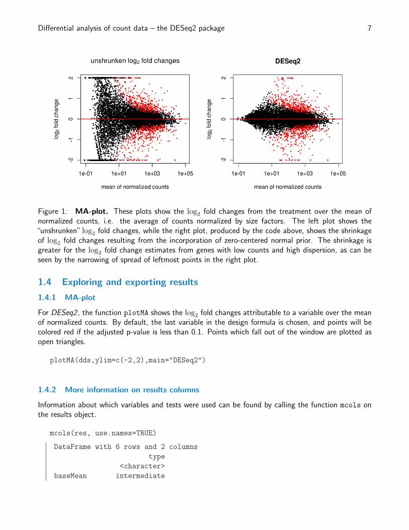
Figure 1: MA-plot. These plots show the log2 fold changes from the treatment over the mean ofnormalized counts, i.e. the average of counts normalized by size factors. The left plot shows the“unshrunken” log2 fold changes, while the right plot, produced by the code above, shows the shrinkageof log2 fold changes resulting from the incorporation of zero-centered normal prior. The shrinkage isgreater for the log2 fold change estimates from genes with low counts and high dispersion, as can beseen by the narrowing of spread of leftmost points in the right plot.
1.4 Exploring and exporting results
1.4.1 MA-plot
For DESeq2 , the function plotMA shows the log2 fold changes attributable to a variable over the meanof normalized counts. By default, the last variable in the design formula is chosen, and points will becolored red if the adjusted p-value is less than 0.1. Points which fall out of the window are plotted asopen triangles.
plotMA(dds,ylim=c(-2,2),main="DESeq2")
1.4.2 More information on results columns
Information about which variables and tests were used can be found by calling the function mcols onthe results object.
mcols(res, use.names=TRUE)
DataFrame with 6 rows and 2 columns
type
<character>
baseMean intermediate

Differential analysis of count data – the DESeq2 package 8
log2FoldChange results
lfcSE results
stat results
pvalue results
padj results
description
<character>
baseMean the base mean over all rows
log2FoldChange log2 fold change (MAP): condition treated vs untreated
lfcSE standard error: condition treated vs untreated
stat Wald statistic: condition treated vs untreated
pvalue Wald test p-value: condition treated vs untreated
padj BH adjusted p-values
The variable condition and the factor level treated are combined as“condition treated vs untreated”.For a particular gene, a log2 fold change of −1 for condition_treated_vs_untreated means thatthe treatment induces a change in observed expression level of 2−1 = 0.5 compared to the untreatedcondition. If the variable of interest is continuous-valued, then the reported log2 fold change is per unitof change of that variable.
The results for particular genes can be set to NA, for either one of the following reasons:1. If within a row, all samples have zero counts, this is recorded in mcols(dds)$allZero and log2
fold change estimates, p-value and adjusted p-value will all be set to NA.2. If a row contains a sample with an extreme count then the p-value and adjusted p-value are set to
NA. These outlier counts are detected by Cook’s distance. Customization of this outlier filteringis described in Section 3.3, along with a method for replacing outlier counts and refitting.
3. If a row is filtered by automatic independent filtering, then only the adjusted p-value is set to NA.Description and customization of independent filtering is decribed in Section 3.6.
1.4.3 Exporting results
An HTML report of the results with plots and sortable/filterable columns can be exported using theReportingTools package (version higher than 2.1.16) on a DESeqDataSet which has been processedby the DESeq function. For a code example, see the “RNA-seq differential expression” vignette at theReportingTools page, or the manual page for the publish method for the DESeqDataSet class.
A plain-text file of the results can be exported using the base R functions write.csv or write.delim,and a descriptive file name indicating the variable which was tested.
write.csv(as.data.frame(res),
file="condition_treated_results.csv")
1.5 Multi-factor designs
Experiments with more than one factor influencing the counts can be analyzed using model formulaewith additional variables. The data in the pasilla package have a condition of interest (the columncondition), as well as the type of sequencing which was performed (the column type).

Differential analysis of count data – the DESeq2 package 9
colData(dds)
DataFrame with 7 rows and 3 columns
condition type sizeFactor
<factor> <factor> <numeric>
treated1fb treated single-read 1.512
treated2fb treated paired-end 0.784
treated3fb treated paired-end 0.896
untreated1fb untreated single-read 1.050
untreated2fb untreated single-read 1.659
untreated3fb untreated paired-end 0.712
untreated4fb untreated paired-end 0.784
We can account for the different types of sequencing, and get a clearer picture of the differencesattributable to the treatment. As condition is the variable of interest, we put it at the end of theformula. Here we
design(dds) <- formula(~ type + condition)
dds <- DESeq(dds)
Again, we access the results using the results function.
res <- results(dds)
head(res)
DataFrame with 6 rows and 6 columns
baseMean log2FoldChange lfcSE stat pvalue padj
<numeric> <numeric> <numeric> <numeric> <numeric> <numeric>
FBgn0000003 0.159 0.0891 0.117 0.7636 0.4451 NA
FBgn0000008 52.226 0.0130 0.252 0.0516 0.9588 0.983
FBgn0000014 0.390 0.0241 0.145 0.1665 0.8677 NA
FBgn0000015 0.905 -0.1229 0.273 -0.4506 0.6523 NA
FBgn0000017 2358.243 -0.2667 0.122 -2.1799 0.0293 0.139
FBgn0000018 221.242 -0.0663 0.124 -0.5357 0.5921 0.824
It is also possible to retrieve the log2 fold changes, p-values and adjusted p-values of the type
variable. The function results takes an argument name, which is a combination of the variable, thelevel (numeratoFr of the fold change) and the base level (denominator of the fold change). In addition,there might be minor changes made by the make.names function on column names, e.g. changing -
(a dash) to . (a period). The function resultsNames will tell you the names of all available results.
resultsNames(dds)
[1] "Intercept" "type_single.read_vs_paired.end"
[3] "condition_treated_vs_untreated"
resType <- results(dds, "type_single.read_vs_paired.end")
head(resType)
Differential analysis of count data – the DESeq2 package 10
DataFrame with 6 rows and 6 columns
baseMean log2FoldChange lfcSE stat pvalue padj
<numeric> <numeric> <numeric> <numeric> <numeric> <numeric>
FBgn0000003 0.159 -0.0686 0.106 -0.6453 0.5188 NA
FBgn0000008 52.226 -0.0808 0.247 -0.3267 0.7439 0.8640
FBgn0000014 0.390 0.0147 0.132 0.1114 0.9113 NA
FBgn0000015 0.905 -0.2222 0.252 -0.8806 0.3785 NA
FBgn0000017 2358.243 0.0081 0.122 0.0665 0.9470 0.9771
FBgn0000018 221.242 0.2954 0.122 2.4212 0.0155 0.0723
mcols(resType)
DataFrame with 6 rows and 2 columns
type description
<character> <character>
1 intermediate the base mean over all rows
2 results log2 fold change (MAP): type single-read vs paired-end
3 results standard error: type single-read vs paired-end
4 results Wald statistic: type single-read vs paired-end
5 results Wald test p-value: type single-read vs paired-end
6 results BH adjusted p-values
2 Data transformations and visualization
2.1 Count data transformations
For testing for differential expression we operate on raw counts and use discrete distributions, howeverfor other downstream analyses – e.g. for visualization or clustering – it might be useful to work withtransformed versions of the count data.
Maybe the most obvious choice of transformation is the logarithm. Since count values for a genecan be zero in some conditions (and non-zero in others), some advocate the use of pseudocounts, i. e.transformations of the form
y = log2(n+ 1) or more generally, y = log2(n+ n0), (1)
where n represents the count values and n0 is a positive constant.In this section, we discuss two alternative approaches that offer more theoretical justification and a
rational way of choosing the parameter equivalent to n0 above. One method incorporates priors on thesample differences, and the other uses the concept of variance stabilizing transformations [3–5].
The two functions, rlogTransformation and varianceStabilizingTransformation, have anargument blind, for whether the transformation should be blind to the sample information specifiedby the design formula. By setting the argument blind to TRUE, the functions will re-estimate thedispersions using only an intercept (design formula ∼ 1). This setting should be used in order tocompare samples in a manner unbiased by the information about experimental groups, for exampleto perform sample QA (quality assurance) as demonstrated below. By setting blind to FALSE, the

Differential analysis of count data – the DESeq2 package 11
dispersions already estimated will be used to perform transformations, or if not present, they will beestimated using the current design formula. This setting should be used for transforming data fordownstream analysis.
The two functions return SummarizedExperiment objects, as the data are no longer counts. Theassay function is used to extract the matrix of normalized values.
rld <- rlogTransformation(dds, blind=TRUE)
vsd <- varianceStabilizingTransformation(dds, blind=TRUE)
2.1.1 Regularized log transformation
The function rlogTransformation, stands for regularized log, transforming the original count data tothe log2 scale by fitting a model with a term for each sample and a prior distribution on the coefficientswhich is estimated from the data. This is very similar to the regularization used by the DESeq andnbinomWaldTest, as seen in Figure 1. The resulting data contains elements defined as:
log2(qij) = xj.βi
where qij is a parameter proportional to the expected true concentration of fragments for gene i andsample j (see Section 4.1), xj. is the j-th row of the design matrix X, which has a 1 for the interceptand a 1 for the sample-specific beta, and βi is the vector of coefficients for gene i. Without priors, thisdesign matrix would lead to a non-unique solution, however the addition of a prior on non-interceptbetas allows for a unique solution to be found. The regularized log transformation is preferable to thevariance stabilizing transformation if the size factors vary widely.
2.1.2 Variance stabilizing transformation
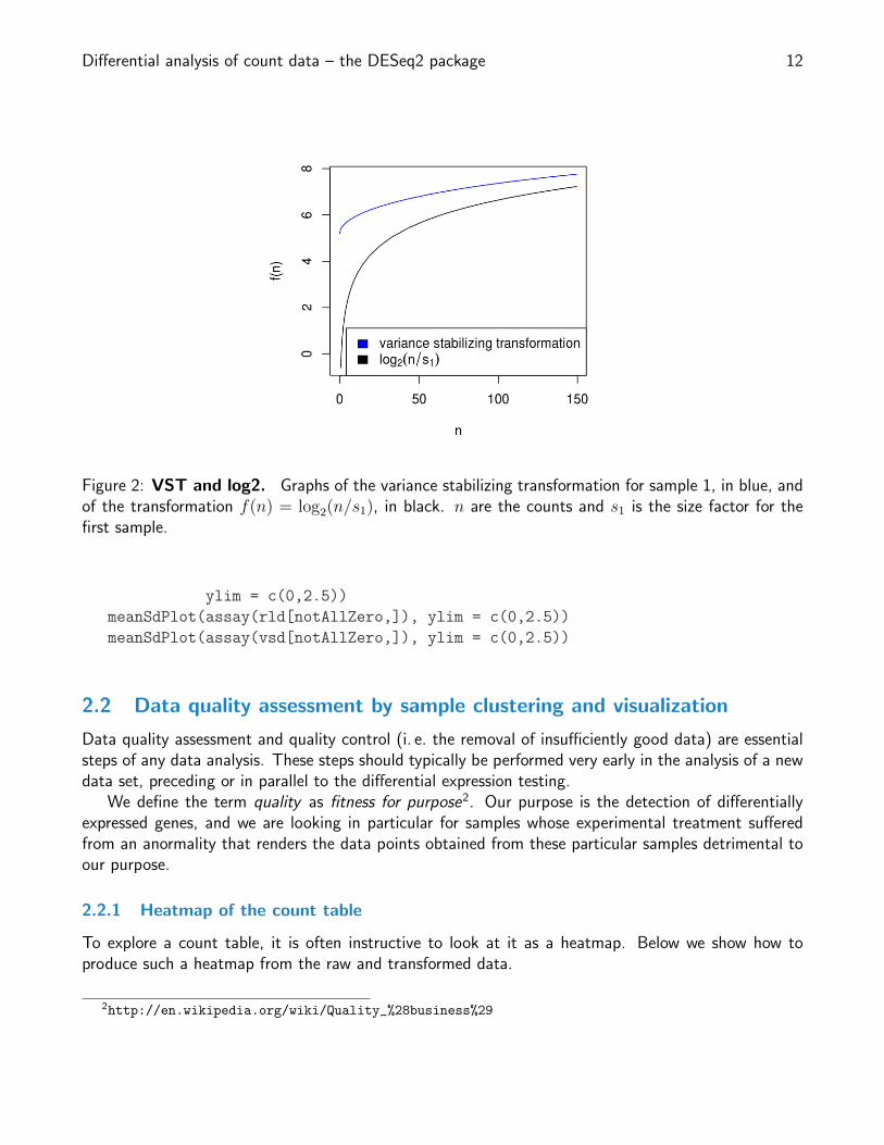
Above, we used a parametric fit for the dispersion. In this case, the closed-form expression for thevariance stabilizing transformation is used by varianceStabilizingTransformation, which is derivedin the file vst.pdf, that is distributed in the package alongside this vignette. If a local fit is used (optionfitType="locfit" to estimateDispersions) a numerical integration is used instead.
The resulting variance stabilizing transformation is shown in Figure 2. The code that produces thefigure is hidden from this vignette for the sake of brevity, but can be seen in the .Rnw or .R source file.
2.1.3 Effects of transformations on the variance
Figure 3 plots the standard deviation of the transformed data, across samples, against the mean, usingthe shifted logarithm transformation (1), the regularized log transformation and the variance stabilizingtransformation. The shifted logarithm has elevated standard deviation in the lower count range, andthe regularized log to a lesser extent, while for the variance stabilized data the standard deviation isroughly constant along the whole dynamic range.
library("vsn")
par(mfrow=c(1,3))
notAllZero <- (rowSums(counts(dds))>0)
meanSdPlot(log2(counts(dds,normalized=TRUE)[notAllZero,] + 1),
Differential analysis of count data – the DESeq2 package 12
Figure 2: VST and log2. Graphs of the variance stabilizing transformation for sample 1, in blue, andof the transformation f(n) = log2(n/s1), in black. n are the counts and s1 is the size factor for thefirst sample.
ylim = c(0,2.5))
meanSdPlot(assay(rld[notAllZero,]), ylim = c(0,2.5))
meanSdPlot(assay(vsd[notAllZero,]), ylim = c(0,2.5))
2.2 Data quality assessment by sample clustering and visualization
Data quality assessment and quality control (i. e. the removal of insufficiently good data) are essentialsteps of any data analysis. These steps should typically be performed very early in the analysis of a newdata set, preceding or in parallel to the differential expression testing.
We define the term quality as fitness for purpose2. Our purpose is the detection of differentiallyexpressed genes, and we are looking in particular for samples whose experimental treatment sufferedfrom an anormality that renders the data points obtained from these particular samples detrimental toour purpose.
2.2.1 Heatmap of the count table
To explore a count table, it is often instructive to look at it as a heatmap. Below we show how toproduce such a heatmap from the raw and transformed data.
2http://en.wikipedia.org/wiki/Quality_%28business%29

Differential analysis of count data – the DESeq2 package 13
Figure 3: Per-gene standard deviation (taken across samples), against the rank of the mean, for theshifted logarithm log2(n+ 1) (left), the regularized log transformation (center) and the variance stabi-lizing transformation (right).
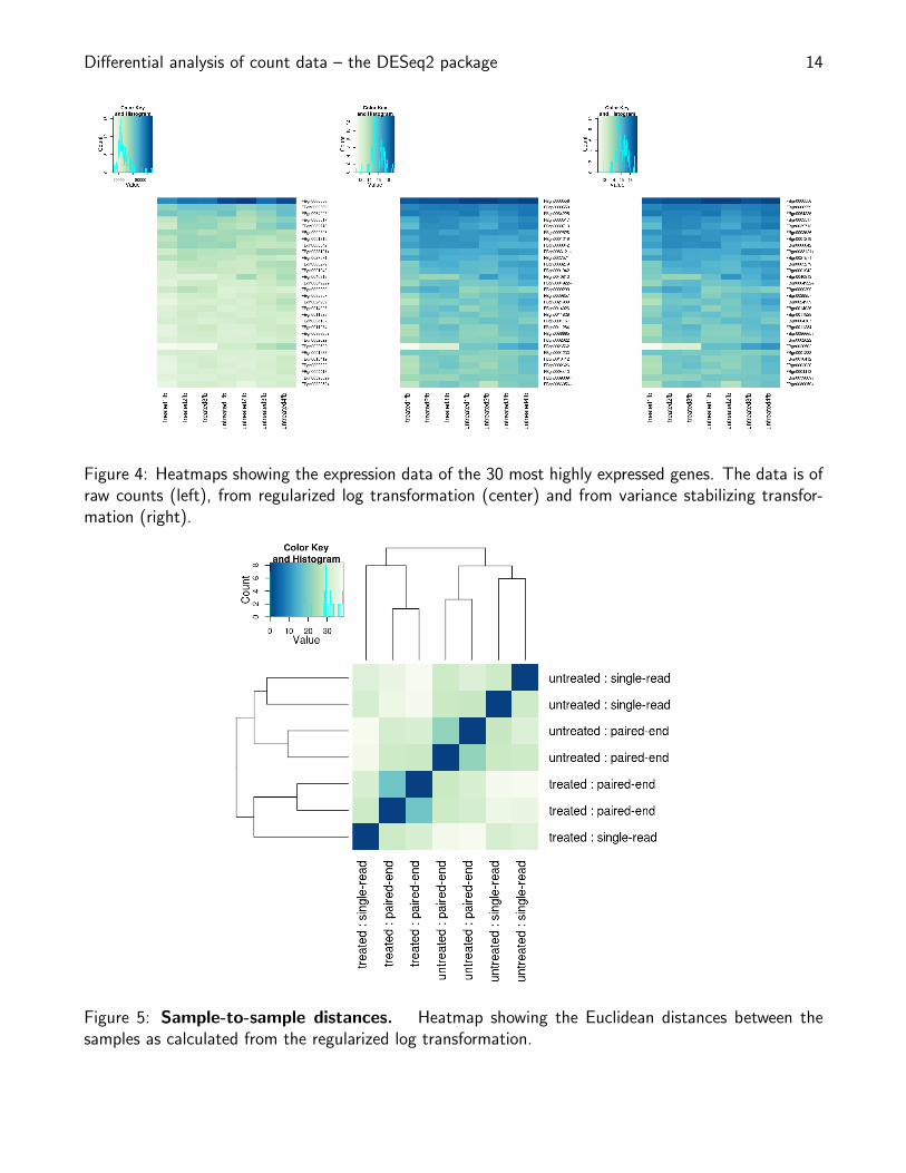
library("RColorBrewer")
library("gplots")
select <- order(rowMeans(counts(dds,normalized=TRUE)),decreasing=TRUE)[1:30]
hmcol <- colorRampPalette(brewer.pal(9, "GnBu"))(100)
heatmap.2(counts(dds,normalized=TRUE)[select,], col = hmcol,
Rowv = FALSE, Colv = FALSE, scale="none",
dendrogram="none", trace="none", margin=c(10,6))
heatmap.2(assay(rld)[select,], col = hmcol,
Rowv = FALSE, Colv = FALSE, scale="none",
dendrogram="none", trace="none", margin=c(10, 6))
heatmap.2(assay(vsd)[select,], col = hmcol,
Rowv = FALSE, Colv = FALSE, scale="none",
dendrogram="none", trace="none", margin=c(10, 6))
2.2.2 Heatmap of the sample-to-sample distances
Another use of the transformed data is sample clustering. Here, we apply the dist function to thetranspose of the transformed count matrix to get sample-to-sample distances. We could alternativelyuse the variance stabilized transformation here.
distsRL <- dist(t(assay(rld)))
Differential analysis of count data – the DESeq2 package 14
Figure 4: Heatmaps showing the expression data of the 30 most highly expressed genes. The data is ofraw counts (left), from regularized log transformation (center) and from variance stabilizing transfor-mation (right).
Figure 5: Sample-to-sample distances. Heatmap showing the Euclidean distances between thesamples as calculated from the regularized log transformation.

Differential analysis of count data – the DESeq2 package 15
Figure 6: PCA plot. PCA plot. The 7 samples shown in the 2D plane spanned by their firsttwo principal components. This type of plot is useful for visualizing the overall effect of experimentalcovariates and batch effects.
A heatmap of this distance matrix gives us an overview over similarities and dissimilarities betweensamples (Figure 5):
mat <- as.matrix(distsRL)
rownames(mat) <- colnames(mat) <- with(colData(dds),
paste(condition, type, sep=" : "))
heatmap.2(mat, trace="none", col = rev(hmcol), margin=c(13, 13))
2.2.3 Principal component plot of the samples
Related to the distance matrix of Section 2.2.2 is the PCA plot of the samples, which we obtain asfollows (Figure 6).
print(plotPCA(rld, intgroup=c("condition", "type")))
Differential analysis of count data – the DESeq2 package 16
3 Variations to the standard workflow
3.1 Wald test individual steps
The function DESeq runs the following functions in order:
dds <- estimateSizeFactors(dds)
dds <- estimateDispersions(dds)
dds <- nbinomWaldTest(dds)
3.2 Contrasts
A contrast is a linear combination of factor level means, which can be used to test if combinationsof variables are different than zero. The simplest use case for contrasts is the case of a factor withthree levels, say A,B and C, where A is the base level. While the standard DESeq2 workflow generatesp-values for the null hypotheses that the log2 fold change of B vs A is zero, and that the log2 foldchange of C vs A is zero, a contrast is needed to compare if the log2 fold change of C vs B is zero.
Here we show how to make all three pairwise comparisons using the parathyroid dataset which wasbuilt in Section 1.2.2. The three levels of the factor treatment are: Control, DPN and OHT. Thesamples are also split according to the patient from which the cell cultures were derived, so we includethis in the design formula.
ddsCtrst <- ddsPara[, colData(ddsPara)$time == "48h"]
as.data.frame(colData(ddsCtrst)[,c("patient","treatment")])
patient treatment
SRR479053 1 Control
SRR479055 1 DPN
SRR479057 1 OHT
SRR479059 2 Control
SRR479062 2 DPN
SRR479065 2 OHT
SRR479067 3 Control
SRR479069 3 DPN
SRR479071 3 OHT
SRR479072 4 Control
SRR479074 4 DPN
SRR479075 4 DPN
SRR479077 4 OHT
SRR479078 4 OHT
design(ddsCtrst) <- ~ patient + treatment
First we run DESeq and show how to extract one of the two comparisons of the treatment factorwith the base level: the comparison of DPN vs Control or the comparison of OHT vs Control.

Differential analysis of count data – the DESeq2 package 17
ddsCtrst <- DESeq(ddsCtrst)
resultsNames(ddsCtrst)
[1] "Intercept" "patient_2_vs_1"
[3] "patient_3_vs_1" "patient_4_vs_1"
[5] "treatment_DPN_vs_Control" "treatment_OHT_vs_Control"
resPara <- results(ddsCtrst,"treatment_OHT_vs_Control")
head(resPara,2)
DataFrame with 2 rows and 6 columns
baseMean log2FoldChange lfcSE stat pvalue
<numeric> <numeric> <numeric> <numeric> <numeric>
ENSG00000000003 515.258 -0.0625 0.0802 -0.779 0.436
ENSG00000000005 0.407 -0.3314 0.5336 -0.621 0.535
padj
<numeric>
ENSG00000000003 0.833
ENSG00000000005 NA
mcols(resPara)
DataFrame with 6 rows and 2 columns
type description
<character> <character>
1 intermediate the base mean over all rows
2 results log2 fold change (MAP): treatment OHT vs Control
3 results standard error: treatment OHT vs Control
4 results Wald statistic: treatment OHT vs Control
5 results Wald test p-value: treatment OHT vs Control
6 results BH adjusted p-values
Using the contrast argument of the results function, we can specify a test of OHT vs DPN.The contrast argument takes a character vector of length three, containing the name of the factor, thename of the numerator level, and the name of the denominator level, where we test the log2 fold changeof numerator vs denominator. Here we extract the results for the log2 fold change of OHT vs DPN forthe treatment factor.
resCtrst <- results(ddsCtrst, contrast=c("treatment","OHT","DPN"))
head(resCtrst,2)
DataFrame with 2 rows and 6 columns
baseMean log2FoldChange lfcSE stat pvalue
<numeric> <numeric> <numeric> <numeric> <numeric>
ENSG00000000003 515.258 -0.0632 0.0752 -0.840 0.401
ENSG00000000005 0.407 -0.4751 0.8284 -0.574 0.566
padj
<numeric>
ENSG00000000003 0.721
ENSG00000000005 NA

Differential analysis of count data – the DESeq2 package 18
mcols(resCtrst)
DataFrame with 6 rows and 2 columns
type description
<character> <character>
1 intermediate the base mean over all rows
2 results log2 fold change (MAP): treatment.OHT.vs.DPN
3 results standard error: treatment.OHT.vs.DPN
4 results Wald statistic: treatment.OHT.vs.DPN
5 results Wald test p-value: treatment.OHT.vs.DPN
6 results BH adjusted p-values
For advanced users, a numeric contrast vector can also be provided with one element for each elementprovided by resultsNames, i.e. columns of the model matrix. Note that the following contrast is thesame as specified by the character vector in the previous code chunk.
resCtrst <- results(ddsCtrst, contrast=c(0,0,0,0,-1,1))
head(resCtrst,2)
DataFrame with 2 rows and 6 columns
baseMean log2FoldChange lfcSE stat pvalue
<numeric> <numeric> <numeric> <numeric> <numeric>
ENSG00000000003 515.258 -0.0632 0.0752 -0.840 0.401
ENSG00000000005 0.407 -0.4751 0.8284 -0.574 0.566
padj
<numeric>
ENSG00000000003 0.721
ENSG00000000005 NA
mcols(resCtrst)
DataFrame with 6 rows and 2 columns
type description
<character> <character>
1 intermediate the base mean over all rows
2 results log2 fold change (MAP): 0,0,0,0,-1,+1
3 results standard error: 0,0,0,0,-1,+1
4 results Wald statistic: 0,0,0,0,-1,+1
5 results Wald test p-value: 0,0,0,0,-1,+1
6 results BH adjusted p-values
The formula that is used to generate the contrasts can be found in Section 4.4.
3.3 Dealing with count outliers
RNA-Seq data sometimes contain isolated instances of very large counts that are apparently unrelatedto the experimental or study design, and which may be considered outliers. There are many reasons whyoutliers can arise, including rare technical or experimental artifacts, read mapping problems in the case
Differential analysis of count data – the DESeq2 package 19
of genetically differing samples, and genuine, but rare biological events. In many cases, users appearprimarily interested in genes that show a consistent behaviour, and this is the reason why by default,genes that are affected by such outliers are set aside by DESeq2 . The function calculates, for everygene and for every sample, a diagnostic test for outliers called Cook’s distance. Cook’s distance is ameasure of how much a single sample is influencing the fitted coefficients for a gene, and a large valueof Cook’s distance is intended to indicate an outlier count. DESeq2 automatically flags genes withCook’s distance above a cutoff and sets their p-values and adjusted p-values to NA.
The default cutoff depends on the sample size and number of parameters to be estimated. Thedefault is to use the 99% quantile of the F (p,m − p) distribution (with p the number of parametersincluding the intercept and m number of samples). The default can be modified using the cooksCut-
off argument to the results function. The outlier removal functionality can be disabled by settingcooksCutoff to FALSE or Inf. If the removal of a sample would mean that a coefficient cannotbe fitted (e.g. if there is only one sample for a given group), then the Cook’s distance for this sam-ple is not counted towards the flagging. The Cook’s distances are stored as a matrix available inassays(dds)[["cooks"]]. These values are the same as those produced by the cooks.distance
function of the stats package, except using the fitted dispersion and taking into account the size factors.With many degrees of freedom –i. e., many more samples than number of parameters to be estimated–
it might be undesirable to remove entire genes from the analysis just because their data include a singlecount outlier. An alternate strategy is to replace the outlier counts with the trimmed mean over allsamples, adjusted by the size factor for that sample. This approach is conservative, it will not leadto false positives, as it replaces the outlier value with the value predicted by the null hypothesis. TheDESeq function (or nbinomWaldTest and nbinomLRT) calculates Cook’s distance for every gene andsample. After an initial fit has been performed, the following function replaces count outliers by thetrimmed mean. Here we demonstrate with the pasilla dataset, although there are not many extradegrees of freedom for this dataset.
ddsClean <- replaceOutliersWithTrimmedMean(dds)
Finally we rerun all the steps of DESeq.
ddsClean <- DESeq(ddsClean)
tab <- table(initial = results(dds)$padj < .1,
cleaned = results(ddsClean)$padj < .1)
addmargins(tab)
cleaned
initial FALSE TRUE Sum
FALSE 6468 4 6472
TRUE 2 1478 1480
Sum 6470 1482 7952
3.4 Likelihood ratio test
One reason to use the likelihood ratio test is in order to test the null hypothesis that log2 fold changesfor multiple levels of a factor, or for multiple variables, such as all interactions between two variables,

Differential analysis of count data – the DESeq2 package 20
are equal to zero. The likelihood ratio test can also be specified using the test argument to DESeq,which substitutes nbinomWaldTest with nbinomLRT. In this case, the user provides the full formula(the formula stored in design(dds)), and a reduced formula, e.g. one which does not contain thevariable of interest. The degrees of freedom for the test is obtained from the number of parametersin the two models. The Wald test and the likelihood ratio test share many of the same genes withadjusted p-value < .1 for this experiment.
As we already have an object dds with dispersions calculated for the design formula type +
condition, we only need to run the function nbinomLRT, with a reduced formula including only thetype of sequencing, in order to test the log2 fold change attributable to the condition:
ddsLRT <- nbinomLRT(dds, reduced = ~ type)
resLRT <- results(ddsLRT)
head(resLRT,2)
DataFrame with 2 rows and 6 columns
baseMean log2FoldChange lfcSE stat pvalue padj
<numeric> <numeric> <numeric> <numeric> <numeric> <numeric>
FBgn0000003 0.159 14.2819 201.782 0.5611 0.454 NA
FBgn0000008 52.226 0.0128 0.294 0.0019 0.965 0.988
mcols(resLRT)
DataFrame with 6 rows and 2 columns
type description
<character> <character>
1 intermediate the base mean over all rows
2 results log2 fold change: condition treated vs untreated
3 results standard error: condition treated vs untreated
4 results LRT statistic: '~ type + condition' vs '~ type'
5 results LRT p-value: '~ type + condition' vs '~ type'
6 results BH adjusted p-values
tab <- table(Wald=res$padj < .1, LRT=resLRT$padj < .1)
addmargins(tab)
LRT
Wald FALSE TRUE Sum
FALSE 6472 5 6477
TRUE 9 1472 1481
Sum 6481 1477 7958
3.5 Dispersion plot and fitting alternatives
Plotting the dispersion estimates is a useful diagnostic. The dispersion plot in Figure 7 is typical, withthe final estimates shrunk from the gene-wise estimates towards the fitted estimates. Some gene-wiseestimates are flagged as outliers and not shrunk towards the fitted value, (this outlier detection isdescribed in the man page for estimateDispersionsMAP). The amount of shrinkage can be more or

Differential analysis of count data – the DESeq2 package 21
Figure 7: Dispersion plot. The dispersion estimate plot shows the gene-wise estimates (black), thefitted values (red), and the final maximum a posteriori estimates used in testing (blue).
less than seen here, depending on the sample size, the number of coefficients, the row mean and thevariability of the gene-wise estimates.
plotDispEsts(dds)
3.5.1 Local dispersion fit
The local dispersion fit is available in case the parametric fit fails to converge. A warning will beprinted that one should use plotDispEsts to check the quality of the fit, whether the curve is pulleddramatically by a few outlier points.
ddsLocal <- estimateDispersions(dds, fitType="local")
3.5.2 Mean dispersion
While RNA-Seq data tend to demonstrate a dispersion-mean dependence, this assumption is not ap-propriate for all assays. An alternative is to use the mean of all gene-wise dispersion estimates.
ddsMean <- estimateDispersions(dds, fitType="mean")

Differential analysis of count data – the DESeq2 package 22
3.5.3 Supply a custom dispersion fit
Any fitted values can be provided during dispersion estimation, using the lower-level functions describedin the manual page for estimateDispersionsGeneEst. In the first line of the code below, the functionestimateDispersionsGeneEst stores the gene-wise estimates in the metadata column dispGeneEst.In the last line, the function estimateDispersionsMAP, uses this column and the column dispFit togenerate maximum a posteriori (MAP) estimates of dispersion. The modeling assumption is that thetrue dispersions are distributed according to a log-normal prior around the fitted values in the columnfitDisp. The width of this prior is calculated from the data.
ddsMed <- estimateDispersionsGeneEst(dds)
useForMedian <- mcols(ddsMed)$dispGeneEst > 1e-7
medianDisp <- median(mcols(ddsMed)$dispGeneEst[useForMedian],na.rm=TRUE)
mcols(ddsMed)$dispFit <- medianDisp
ddsMed <- estimateDispersionsMAP(ddsMed)
3.6 Independent filtering of results
The results function of the DESeq2 package performs independent filtering by default using the meanof normalized counts as a filter statistic. A threshold on the filter statistic is found which optimizesthe number of adjusted p-values lower than a significance level alpha (we use the standard variablename for significance level, though it is unrelated to the dispersion parameter α). The theory behindindependent filtering is discussed in greater detail in Section 4.5. The adjusted p-values for the geneswhich do not pass the filter threshold are set to NA.
The independent filtering is performed using the filtered_p function of the genefilter package,and all of the arguments of filtered_p can be passed to the results function. The filter thresholdvalue and the number of rejections at each quantile of the filter statistic are available as attributes ofthe object returned by results. For example, we can easily visualize the optimization by plotting thefilterNumRej attribute of the results object, as seen in Figure 8.
attr(res,"filterThreshold")
45%
6.85
plot(attr(res,"filterNumRej"),type="b",
ylab="number of rejections")
Independent filtering can be turned off by setting independentFiltering to FALSE. Alternativefiltering statistics can be easily provided as an argument to the results function.
resNoFilt <- results(dds, independentFiltering=FALSE)
table(filtering=(res$padj < .1), noFiltering=(resNoFilt$padj < .1))
noFiltering
filtering FALSE TRUE
FALSE 6477 0
TRUE 208 1273

Differential analysis of count data – the DESeq2 package 23
Figure 8: Independent filtering. The results function maximizes the number of rejections (adjustedp-value less than a significance level), over theta, the quantiles of a filtering statistic (in this case, themean of normalized counts).
library(genefilter)
rv <- rowVars(counts(dds,normalized=TRUE))
resFiltByVar <- results(dds, filter=rv)
table(rowMean=(res$padj < .1), rowVar=(resFiltByVar$padj < .1))
rowVar
rowMean FALSE TRUE
FALSE 6315 6
TRUE 0 1481
3.7 Access to all calculated values
All row-wise calculated values (intermediate dispersion calculations, coefficients, standard errors, etc.)are stored in the DESeqDataSet object, e.g. dds in this vignette. These values are accessible by callingmcols on dds. Descriptions of the columns are accessible by two calls to mcols.
mcols(dds,use.names=TRUE)[1:4,1:4]
DataFrame with 4 rows and 4 columns
baseMean baseVar allZero dispGeneEst
Differential analysis of count data – the DESeq2 package 24
<numeric> <numeric> <logical> <numeric>
FBgn0000003 0.159 0.178 FALSE 3.49e-01
FBgn0000008 52.226 154.611 FALSE 5.12e-02
FBgn0000014 0.390 0.444 FALSE 1.44e+01
FBgn0000015 0.905 0.799 FALSE 1.00e-08
mcols(mcols(dds), use.names=TRUE)[1:4,]
DataFrame with 4 rows and 2 columns
type description
<character> <character>
baseMean intermediate the base mean over all rows
baseVar intermediate the base variance over all rows
allZero intermediate all counts in a row are zero
dispGeneEst intermediate gene-wise estimates of dispersion
3.8 Sample-/gene-dependent normalization factors
In some experiments, there might be gene-dependent dependencies which vary across samples. Forinstance, GC-content bias or length bias might vary across samples coming from different labs orprocessed at different times. We use the terms“normalization factors”for a gene × sample matrix, and“size factors” for a single number per sample. Incorporating normalization factors, the mean parameterµij from Section 4.1 becomes:
µij = NFijqij
with normalization factor matrix NF having the same dimensions as the counts matrix K. Thismatrix can be incorporated as shown below. We recommend providing a matrix with a mean of 1, whichcan be accomplished by dividing out the mean of the matrix.
normFactors <- normFactors / mean(normFactors)
normalizationFactors(dds) <- normFactors
These steps then replace estimateSizeFactors in the steps described in Section 3.1. Normaliza-tion factors, if present, will always be used in the place of size factors.
The methods provided by the cqn or EDASeq packages can help correct for GC or length biases.They both describe in their vignettes how to create matrices which can be used by DESeq2 . From theformula above, we see that normalization factors should be on the scale of the counts, like size factors,and unlike offsets which are typically on the scale of the predictors (i.e. the logarithmic scale for thenegative binomial GLM). At the time of writing, the transformation from the matrices provided by thesepackages should be:
cqnOffset <- cqnObject$glm.offset
cqnNormFactors <- exp(cqnOffset)
EDASeqNormFactors <- exp(-1 * EDASeqOffset)

Differential analysis of count data – the DESeq2 package 25
4 Theory behind DESeq2
4.1 Generalized linear model
The differential expression analysis in DESeq2 uses a generalized linear model of the form:
Kij ∼ NB(µij, αi)
µij = sjqij
log2(qij) = xj.βi
where counts Kij for gene i, sample j are modeled using a negative binomial distribution with fittedmean µij and a gene-specific dispersion parameter αi. The fitted mean is composed of a sample-specificsize factor sj
3 and a parameter qij proportional to the expected true concentration of fragments forsample j. The coefficients βi give the log2 fold changes for gene i for each column of the model matrixX. Dispersions are estimated using a Cox-Reid adjusted profile likelihood, as first implemented forRNA-Seq data in edgeR [6, 7]. For further details on dispersion estimation and inference, please seethe manual pages for the functions DESeq and estimateDispersions. For access to the calculatedvalues see Section 3.7
4.2 Changes compared to the DESeq package
The main changes in the package DESeq2 , compared to the (older) version DESeq, are as follows:� SummarizedExperiment is used as the superclass for storage of input data, intermediate calcula-
tions and results.� Maximum a posteriori estimation of GLM coefficients incorporating a zero-mean normal prior with
variance estimated from data (equivalent to Tikhonov/ridge regularization). This adjustment haslittle effect on genes with high counts, yet it helps to moderate the otherwise large spread in log2
fold changes for genes with low counts (e. g. single digits per condition).� Maximum a posteriori estimation of dispersion replaces the sharingMode options fit-only ormaximum of the previous version of the package. [8]
� All estimation and inference is based on the generalized linear model, which includes the twocondition case (previously the exact test was used).
� The Wald test for significance of GLM coefficients is provided as the default inference method,with the likelihood ratio test of the previous version still available.
� It is possible to provide a matrix of sample-/gene-dependent normalization factors.
4.3 Count outlier detection
DESeq2 relies on the negative binomial distribution to make estimates and perform statistical inferenceon differences. While the negative binomial is versatile in having a mean and dispersion parameter,extreme counts in individual samples might not fit well to the negative binomial. For this reason, weperform automatic detection of count outliers. We use Cook’s distance, which is a measure of howmuch the fitted coefficients would change if an individual sample were removed [9]. For more on the
3The model can be generalised to use sample- and gene-dependent normalisation factors, see Appendix 3.8.

Differential analysis of count data – the DESeq2 package 26
Figure 9: Cook’s distance. Plot of the maximum Cook’s distance per gene over the rank of the Waldstatistics for the condition. The two regions with small Cook’s distances are genes with a single countin one sample. The horizontal line is the default cutoff used for 7 samples and 3 estimated parameters.
implementation of Cook’s distance see Section 3.3 and the manual page for the results function.Below we plot the maximum value of Cook’s distance for each row over the rank of the test statisticto justify its use as a filtering criterion.
W <- mcols(dds)$WaldStatistic_condition_treated_vs_untreated
maxCooks <- apply(assays(dds)[["cooks"]],1,max)
idx <- !is.na(W)
plot(rank(W[idx]), maxCooks[idx], xlab="rank of Wald statistic",
ylab="maximum Cook's distance per gene",
ylim=c(0,5), cex=.4, col=rgb(0,0,0,.3))
m <- ncol(dds)
p <- 3
abline(h=qf(.99, p, m - p))
4.4 Contrasts
Contrasts can be calculated for a DESeqDataSet object for which the GLM coefficients have alreadybeen fit using the Wald test steps (DESeq with test="Wald" or using nbinomWaldTest). The vectorof coefficients β is left multiplied by the contrast vector c to form the numerator of the test statistic.

Differential analysis of count data – the DESeq2 package 27
The denominator is formed by multiplying the covariance matrix Σ for the coefficients on either sideby the contrast vector c. The square root of this product is an estimate of the standard error for thecontrast. The contrast statistic is then compared to a normal distribution as are the Wald statistics forthe DESeq2 package.
W =ctβ√ctΣc
4.5 Independent filtering and multiple testing
4.5.1 Filtering criteria
The goal of independent filtering is to filter out those tests from the procedure that have no, or littlechance of showing significant evidence, without even looking at their test statistic. Typically, this resultsin increased detection power at the same experiment-wide type I error. Here, we measure experiment-wide type I error in terms of the false discovery rate.
A good choice for a filtering criterion is one that1. is statistically independent from the test statistic under the null hypothesis,2. is correlated with the test statistic under the alternative, and3. does not notably change the dependence structure –if there is any– between the tests that pass
the filter, compared to the dependence structure between the tests before filtering.The benefit from filtering relies on property 2, and we will explore it further in Section 4.5.2. Its
statistical validity relies on property 1 – which is simple to formally prove for many combinations offilter criteria with test statistics– and 3, which is less easy to theoretically imply from first principles,but rarely a problem in practice. We refer to [10] for further discussion of this topic.
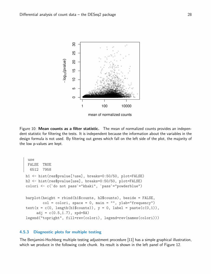
A simple filtering criterion readily available in the results object is the mean of normalized countsirrespective of biological condition (Figure 10). Genes with very low counts are not likely to see significantdifferences typically due to high dispersion. For example, we can plot the − log10 p-values from all genesover the normalized mean counts.
plot(res$baseMean+1, -log10(res$pvalue),
log="x", xlab="mean of normalized counts",
ylab=expression(-log[10](pvalue)),
ylim=c(0,30),
cex=.4, col=rgb(0,0,0,.3))
4.5.2 Why does it work?
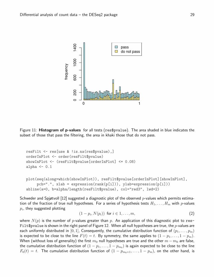
Consider the p value histogram in Figure 11. It shows how the filtering ameliorates the multiple testingproblem – and thus the severity of a multiple testing adjustment – by removing a background set ofhypotheses whose p values are distributed more or less uniformly in [0, 1].
use <- res$baseMean > attr(res,"filterThreshold")
table(use)
Differential analysis of count data – the DESeq2 package 28
Figure 10: Mean counts as a filter statistic. The mean of normalized counts provides an indepen-dent statistic for filtering the tests. It is independent because the information about the variables in thedesign formula is not used. By filtering out genes which fall on the left side of the plot, the majority ofthe low p-values are kept.
use
FALSE TRUE
6512 7958
h1 <- hist(res$pvalue[!use], breaks=0:50/50, plot=FALSE)
h2 <- hist(res$pvalue[use], breaks=0:50/50, plot=FALSE)
colori <- c(`do not pass`="khaki", `pass`="powderblue")
barplot(height = rbind(h1$counts, h2$counts), beside = FALSE,
col = colori, space = 0, main = "", ylab="frequency")
text(x = c(0, length(h1$counts)), y = 0, label = paste(c(0,1)),
adj = c(0.5,1.7), xpd=NA)
legend("topright", fill=rev(colori), legend=rev(names(colori)))
4.5.3 Diagnostic plots for multiple testing
The Benjamini-Hochberg multiple testing adjustment procedure [11] has a simple graphical illustration,which we produce in the following code chunk. Its result is shown in the left panel of Figure 12.
Differential analysis of count data – the DESeq2 package 29
Figure 11: Histogram of p-values for all tests (res$pvalue). The area shaded in blue indicates thesubset of those that pass the filtering, the area in khaki those that do not pass.
resFilt <- res[use & !is.na(res$pvalue),]
orderInPlot <- order(resFilt$pvalue)
showInPlot <- (resFilt$pvalue[orderInPlot] <= 0.08)
alpha <- 0.1
plot(seq(along=which(showInPlot)), resFilt$pvalue[orderInPlot][showInPlot],
pch=".", xlab = expression(rank(p[i])), ylab=expression(p[i]))
abline(a=0, b=alpha/length(resFilt$pvalue), col="red3", lwd=2)
Schweder and Spjøtvoll [12] suggested a diagnostic plot of the observed p-values which permits estima-tion of the fraction of true null hypotheses. For a series of hypothesis tests H1, . . . , Hm with p-valuespi, they suggested plotting
(1− pi, N(pi)) for i ∈ 1, . . . ,m, (2)
where N(p) is the number of p-values greater than p. An application of this diagnostic plot to res-
Filt$pvalue is shown in the right panel of Figure 12. When all null hypotheses are true, the p-values areeach uniformly distributed in [0, 1], Consequently, the cumulative distribution function of (p1, . . . , pm)is expected to be close to the line F (t) = t. By symmetry, the same applies to (1 − p1, . . . , 1 − pm).When (without loss of generality) the first m0 null hypotheses are true and the other m−m0 are false,the cumulative distribution function of (1 − p1, . . . , 1 − pm0) is again expected to be close to the lineF0(t) = t. The cumulative distribution function of (1 − pm0+1, . . . , 1 − pm), on the other hand, is

Differential analysis of count data – the DESeq2 package 30
expected to be close to a function F1(t) which stays below F0 but shows a steep increase towards 1as t approaches 1. In practice, we do not know which of the null hypotheses are true, so we can onlyobserve a mixture whose cumulative distribution function is expected to be close to
F (t) =m0
mF0(t) +
m−m0
mF1(t). (3)
Such a situation is shown in the right panel of Figure 12. If F1(t)/F0(t) is small for small t, then themixture fraction m0
mcan be estimated by fitting a line to the left-hand portion of the plot, and then
noting its height on the right. Such a fit is shown by the red line in the right panel of Figure 12.
plot(1-resFilt$pvalue[orderInPlot],
(length(resFilt$pvalue)-1):0, pch=".",
xlab=expression(1-p[i]), ylab=expression(N(p[i])))
abline(a=0, slope, col="red3", lwd=2)
Figure 12: Left: illustration of the Benjamini-Hochberg multiple testing adjustment procedure [11].The black line shows the p-values (y-axis) versus their rank (x-axis), starting with the smallest p-valuefrom the left, then the second smallest, and so on. Only the first 2300 p-values are shown. The redline is a straight line with slope α/n, where n = 7958 is the number of tests, and α = 0.1 is a targetfalse discovery rate (FDR). FDR is controlled at the value α if the genes are selected that lie to theleft of the rightmost intersection between the red and black lines: here, this results in 1481 genes.Right: Schweder and Spjøtvoll plot, as described in the text. For both of these plots, the p-valuesresFilt$pvalues from Section 4.5.1 were used as a starting point. Analogously, one can producethese types of plots for any set of p-values, for instance those from the previous sections.

Differential analysis of count data – the DESeq2 package 31
5 Frequently asked questions
5.1 How should I email a question?
We welcome emails with questions about our software, and want to ensure that we eliminate issues ifand when they appear. We have a few requests to optimize the process:
� all emails and follow-up questions should take place over the Bioconductor list, which serves as arepository of information and helps saves the developers’ time in responding to similar questions.The subject line should contain “DESeq2” and a few words describing the problem.
� first search the Bioconductor list, http://bioconductor.org/help/mailing-list/, for pastthreads which might have answered your question.
� if you have a question about the behavior of a function, read the sections of the manual page forthis function by typing a question mark and the function name, e.g. ?results. We spend a lotof time documenting individual functions and the exact steps that the software is performing.
� include all of your R code, especially the creation of the DESeqDataSet and the design formula.Include complete warning or error messages, and conclude your message with the full output ofsessionInfo().
� if possible, include the output of as.data.frame(colData(dds)), so that we can have a senseof the experimental setup. If this contains confidential information, you can replace the levels ofthose factors using levels().
5.2 Why are some p-values set to NA?
See the details in Section 1.4.2.
5.3 How do I use the variance stabilized or rlog transformed data for dif-ferential testing?
The variance stabilizing and rlog transformations are provided for applications other than differentialtesting, for example clustering of samples or other machine learning applications. For differential testingwe recommend the DESeq function applied to raw counts as outlined in Section 1.3.
6 Session Info
� R version 3.0.2 Patched (2013-12-18 r64488), x86_64-unknown-linux-gnu� Locale: LC_CTYPE=en_US.UTF-8, LC_NUMERIC=C, LC_TIME=en_US.UTF-8, LC_COLLATE=C,LC_MONETARY=en_US.UTF-8, LC_MESSAGES=en_US.UTF-8, LC_PAPER=en_US.UTF-8,LC_NAME=C, LC_ADDRESS=C, LC_TELEPHONE=C, LC_MEASUREMENT=en_US.UTF-8,LC_IDENTIFICATION=C
� Base packages: base, datasets, grDevices, graphics, methods, parallel, stats, utils� Other packages: Biobase 2.22.0, BiocGenerics 0.8.0, DESeq2 1.2.10, GenomicRanges 1.14.4,
IRanges 1.20.6, RColorBrewer 1.0-5, Rcpp 0.11.0, RcppArmadillo 0.4.000.2, XVector 0.2.0,genefilter 1.44.0, gplots 2.12.1, parathyroidSE 1.0.4, pasilla 0.2.19, vsn 3.30.0

Differential analysis of count data – the DESeq2 package 32
� Loaded via a namespace (and not attached): AnnotationDbi 1.24.0, BiocInstaller 1.12.0,BiocStyle 1.0.0, DBI 0.2-7, DESeq 1.14.0, KernSmooth 2.23-10, RSQLite 0.11.4, XML 3.98-1.1,affy 1.40.0, affyio 1.30.0, annotate 1.40.0, bitops 1.0-6, caTools 1.16, gdata 2.13.2,geneplotter 1.40.0, grid 3.0.2, gtools 3.2.1, lattice 0.20-24, limma 3.18.10, locfit 1.5-9.1,preprocessCore 1.24.0, splines 3.0.2, stats4 3.0.2, survival 2.37-7, tools 3.0.2, xtable 1.7-1,zlibbioc 1.8.0
References
[1] Felix Haglund, Ran Ma, Mikael Huss, Luqman Sulaiman, Ming Lu, Inga-Lena Nilsson, AndersHoog, Christofer C. Juhlin, Johan Hartman, and Catharina Larsson. Evidence of a FunctionalEstrogen Receptor in Parathyroid Adenomas. Journal of Clinical Endocrinology & Metabolism,September 2012.
[2] A. N. Brooks, L. Yang, M. O. Duff, K. D. Hansen, J. W. Park, S. Dudoit, S. E. Brenner, and B. R.Graveley. Conservation of an RNA regulatory map between Drosophila and mammals. GenomeResearch, pages 193–202, 2011.
[3] Robert Tibshirani. Estimating transformations for regression via additivity and variance stabiliza-tion. Journal of the American Statistical Association, 83:394–405, 1988.
[4] Wolfgang Huber, Anja von Heydebreck, Holger Sultmann, Annemarie Poustka, and Martin Vingron.Parameter estimation for the calibration and variance stabilization of microarray data. StatisticalApplications in Genetics and Molecular Biology, 2(1):Article 3, 2003.
[5] Simon Anders and Wolfgang Huber. Differential expression analysis for sequence count data.Genome Biology, 11:R106, 2010.
[6] D. R. Cox and N. Reid. Parameter orthogonality and approximate conditional inference. Journalof the Royal Statistical Society, Series B, 49(1):1–39, 1987.
[7] Davis J McCarthy, Yunshun Chen, and Gordon K Smyth. Differential expression analysis of multi-factor RNA-Seq experiments with respect to biological variation. Nucleic Acids Research, 40:4288–4297, January 2012.
[8] Hao Wu, Chi Wang, and Zhijin Wu. A new shrinkage estimator for dispersion improves differentialexpression detection in RNA-seq data. Biostatistics, September 2012.
[9] R. Dennis Cook. Detection of Influential Observation in Linear Regression. Technometrics, February1977.
[10] Richard Bourgon, Robert Gentleman, and Wolfgang Huber. Independent filtering increases detec-tion power for high-throughput experiments. PNAS, 107(21):9546–9551, 2010.
[11] Y. Benjamini and Y. Hochberg. Controlling the false discovery rate: a practical and powerfulapproach to multiple testing. Journal of the Royal Statistical Society B, 57:289–300, 1995.

Differential analysis of count data – the DESeq2 package 33
[12] T. Schweder and E. Spjotvoll. Plots of P-values to evaluate many tests simultaneously. Biometrika,69:493–502, 1982.